OceanTracker 0.5: fast adaptable Lagrangian particle tracking in structured and unstructured grids

Particle tracking is frequently used to compute particle movements within hydrodynamic ocean models; however, modelling millions of particles is computationally challenging. OceanTracker is designed to reduce the time required to obtain results from particle tracking. Firstly, OceanTracker is computationally efficient, allowing users to simulate large numbers of particles in complex coastal environments, enabling improved statistics and exploration of a wider range of cases within acceptable run times. Secondly, OceanTracker can calculate multiple particle statistics during the computational run, eliminating the need to record and post-process large volumes of particle trajectories. The adaptability of OceanTracker's modular computational pipeline allows users to add and modify components that govern particle physics, behaviour, and statistics. The computational pipeline is entirely assembled from user-provided parameters, supplied as a JSON or YMAL text file or built using helper methods. Coders can easily modify existing components through code inheritance. Currently, OceanTracker supports hydrodynamic model output both for unstructured (SCHISM, FVCOM, DELFT3D-FM) and structured (ROMS, NEMO/GLORYS) grids. Computing the trajectories for more than one million particles with OceanTracker on a single computer core is more than ten times faster than the OpenDrift code and twice as fast as the Parcels code, despite treating structured grids as unstructured, which might be expected to be computationally slower than structured grids due to the time required to locate each particle within a hydrodynamic grid cell. In addition to its single-core performance, OceanTracker can run computations in parallel across available cores. This can further increase speed by up to an order of magnitude on currently available multicore desktop processors.

1 Introduction

Particle tracking is key to answering many scientific and practical questions about physical and biophysical transport in the ocean (Lynch et al., 2014; Van Sebille et al., 2018; Garnier et al., 2025), such as dispersal of pollutants (Ainsworth et al., 2021), movements of larvae, residence times (Lucas and Deleersnijder, 2020), or quantifying connectivity between regions (Atalah et al., 2022). However, a major challenge for particle-tracking models is simulating millions of particles to enable statistically significant results – particularly when introducing stochastic movements in the models to account for uncertainties in the physical currents or biological traits (Van Sebille et al., 2018; Simons et al., 2013; Chaput et al., 2022). This is especially important when estimating the bio-physical connectivities of rare events, such as for the initial arrival of invasive species, which have significant ecological and economic consequences. In these cases, it is necessary to release large numbers of particles to represent the numerous trajectories in the system.

Simulating millions of particles creates several challenges. The first, computing particle trajectories in user-acceptable time frames. This first challenge may result in users either choosing to simulating smaller numbers of particles producing unreliable statistics or shifting their research question to a simplified problem, in order to get results within project deadlines on accessible hardware. The second challenge, is the time required to post-process the trajectories to obtain the required particle statistics (see Sect. 3.1). A third challenge is creating code that is easy to use and yet adaptable to many use cases, e.g. for different particle behaviours. The offline particle tracker OceanTracker addresses all three challenges. However, what constitutes large numbers and acceptable time frames to obtain particle statistics depends on a user's objectives, their computer hardware and project deadlines.

Particle tracking code OceanTracker addresses the first challenge of speed by computing large numbers of particle trajectories with widely accessible desktop and laptop hardware. Table 1 shows a range of hardware, all of which can compute one month of particle trajectories for 1 million particles in 4 to 20 min, depending on the number of processors and their clock speed, see Table 1. The second challenge is a result of the time and effort required to analyse these trajectories and produce the required particle statistics, which includes the logistical challenges of storing and accessing what can be terabytes of data. This new version, OceanTracker 0.5, can resolve some of these issues by recording particle statistics during the computational run, e.g. heat maps and connectivities between regions, as shown in Fig. 1 and Sect. 4.8. On-the-fly statistics may address both the post-processing time and storage issues, as no particle trajectories need to be recorded, and the size of the statistical output files is independent of the number of particles released. If required, individual particle trajectories can also be recorded to allow detailed inspection of results. However, including the full-time resolution of the trajectories in any statistical computations would require recording every time step. On-the-fly statistics can enable full-time resolution without the cost of writing to disk at every time step.

The aspects of adaptability addressed in this work are two fold. First, for most users it is simple to incorporate their required particle behaviours from a suite of supplied options using a configuration file. Second, coding users can easily extend and adapt the given options to meet their specialised needs. The new modular computational pipeline in OceanTracker 0.5 addresses aspects of the third challenge of adaptability by structuring the computational pipeline as a sequence of discrete steps, each responsible for a specific computational task, see Fig. 3. Users add tasks as components within roles. These components are dynamically assembled at runtime to create the required computational pipeline. Components may be those supplied by OceanTracker or the user. In many cases multiple components can be added to the same role. For example, there can be multiple release groups, each with distinct release locations and schedules, or multiple biophysical behaviours that alter particle trajectories (e.g., larvae settling within a defined area and time period (Demmer et al., 2022)). All components are implemented as Python classes, which enables coders to inherit and adapt any in-built component to their specific needs with minimal addtional code.

To allow non-coders to use OceanTracker 0.5 it builds the entire computational pipeline from a user-supplied configuration file. This configuration defines which components are added to roles within the computational pipeline. Alternatively, coders can add components using simple method calls. For each component, the configuration also describes the parameters that specify their individual settings, Sect. 4.1.1. Figure 4 gives a minimal example of these approaches, with the same run done using coding, or from parameters supplied in JSON or YAML text file formats. An additional advantage of using text file parameters is that it allows web-based on-demand particle tracking services to easily access the same level of computational pipeline flexibility (Vennell et al., 2019).

A single particle tracking framework that operates with both structured and unstructured hydrodymamic model grids simplifies the particle tracking process for users by having a uniform approach regardless of which hydrodynamic model is used. Particle trackers for unstructured grids are rare due to the complexity involved in coding the movement and interpolations within the grid. A review of ocean Lagrangian analysis (Van Sebille et al., 2018) lists 11 particle trackers, of which only one “LIGHT in MPAS-O” is capable of working with unstructured grids. Beyond this list, those compatible with both types of grids are even rarer, e.g. OpenDrift (Dagestad et al., 2018), Pylag (Uncles et al., 2020) and the alpha release of Parcels v4. A secondary goal for OceanTracker 0.5 is to provide a single framework that auto-detects the type of grid from multiple hydrodynamic model formats and identifies if useful fields are in the hindcast, such as bottom stress used in particle re-suspension. This enables users to focus on the outcomes they need from particle tracking, rather than the details of the underlying hydrodynamic model's grid and outputs. While OceanTracker version 0.1 only supported the SCHISM hydrodynamic model output format, OceanTracker 0.5 now supports SCHISM, FVCOM, DEFLT3D-FM, NEMO/GLORYS and ROMS formats (Zhang et al., 2016; Lai et al., 2010; O’Shea and Murphy, 2020; Moore et al., 2011). OceanTracker has been applied to a range of studies involving particle-based simulations to understand transport processes in marine environments. These applications typically involve releasing large numbers of particles, tracking their movement over time and then analysing connectivity patterns. Examples include:

• Investigating phytoplankton retention in an estuary. A simulation with one billion particles (up to one million active at any time) modelling population growth through particle splitting and retention mechanisms using a 32k node hindcast (Steidle and Vennell, 2023).

• Inferring the dispersal area of eDNA. Inferring the spatial extent of a species' environmental DNA that may be detected from water samples, within a 155k node hindcast (Pastor Rollan et al., 2024).

• Assessing invasive species risk from ballast water discharge. Modelling the transport of invasive species larvae by releasing 65 million particles from vessels along coastal shipping routes, within a 78k node hindcast(Smeaton et al., 2026).

• Disease spread in aquaculture farms. Estimating connectivity between 500 aquaculture farms by analysing tracks of 150 million particles to determine potential disease transmission pathways, within a 150k node hindcast (Knight et al., 2025).

• Public engagement, online ocean plastics tracker. A web-based tool that allows users to drop virtual plastic and instantly visualise where it travels, returning 20 particle trajectories in less than one second, using a 78k node hindcast (Vennell et al., 2019).

High level goals for this new version of OceanTracker included: (1) deskilling particle tracking for novice users, (2) enabling large particle numbers using laptop and desktop hardware, (3) providing a range of inbuilt options that cover many intermediate user requirements, and (4) allowing experienced coders to extend existing options with minimal additional code. OceanTracker's modular approach, auto-detection of readers, algorithmic efficiency and automation within OceanTracker contribute to these goals (see Sect. 4.1, 4.4 and 4.1.3, and the minimal example in Fig. 4).

This paper provides a high-level outline of the features and structure of the updates to OceanTracker since the release of version 0.1 (Vennell et al., 2021), so they can better understand the framework within which they assemble their computational pipeline. The paper only includes brief comments on how key aspects were implemented within the OceanTracker code, as this will require a future more technically focused paper.

An overview of OceanTracker's features is provided in Sect. 3, including some example outputs in Fig. 1. Section 4 details its structure, and a description of how to configure the computational pipeline is given in Sect. 4.1.1. Additionally, Sect. 4.9 outlines integrated models that combine components within roles to achieve higher-level functionality, such as calculating Lagrangian coherent structures. Section 5 explores the features contributing to OceanTracker's computational speed and compares its performance to OpenDrift and Parcels.

Table 1 OceanTracker run times for modelling 1 million particles over a period of 1 month. Each run utilised all physical computer cores and completed 2880 time steps of 15 min each using 4th order Runge-Kutta time integration in 3D. The unstructured hydrodynamic model had 79k nodes and 140k triangles. Read times are the time spent reading the hindcast from the local disk, with the balance of time spent computing particle tracks.

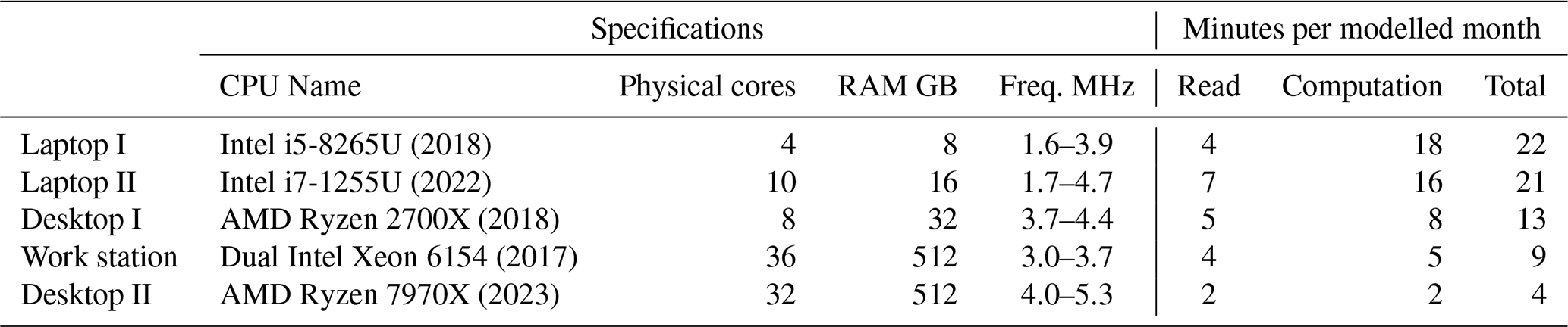
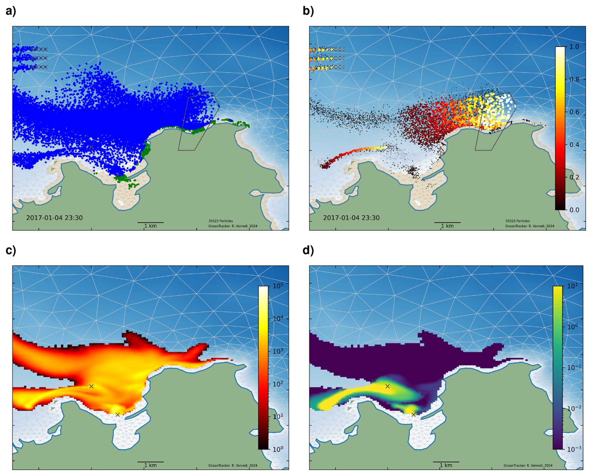
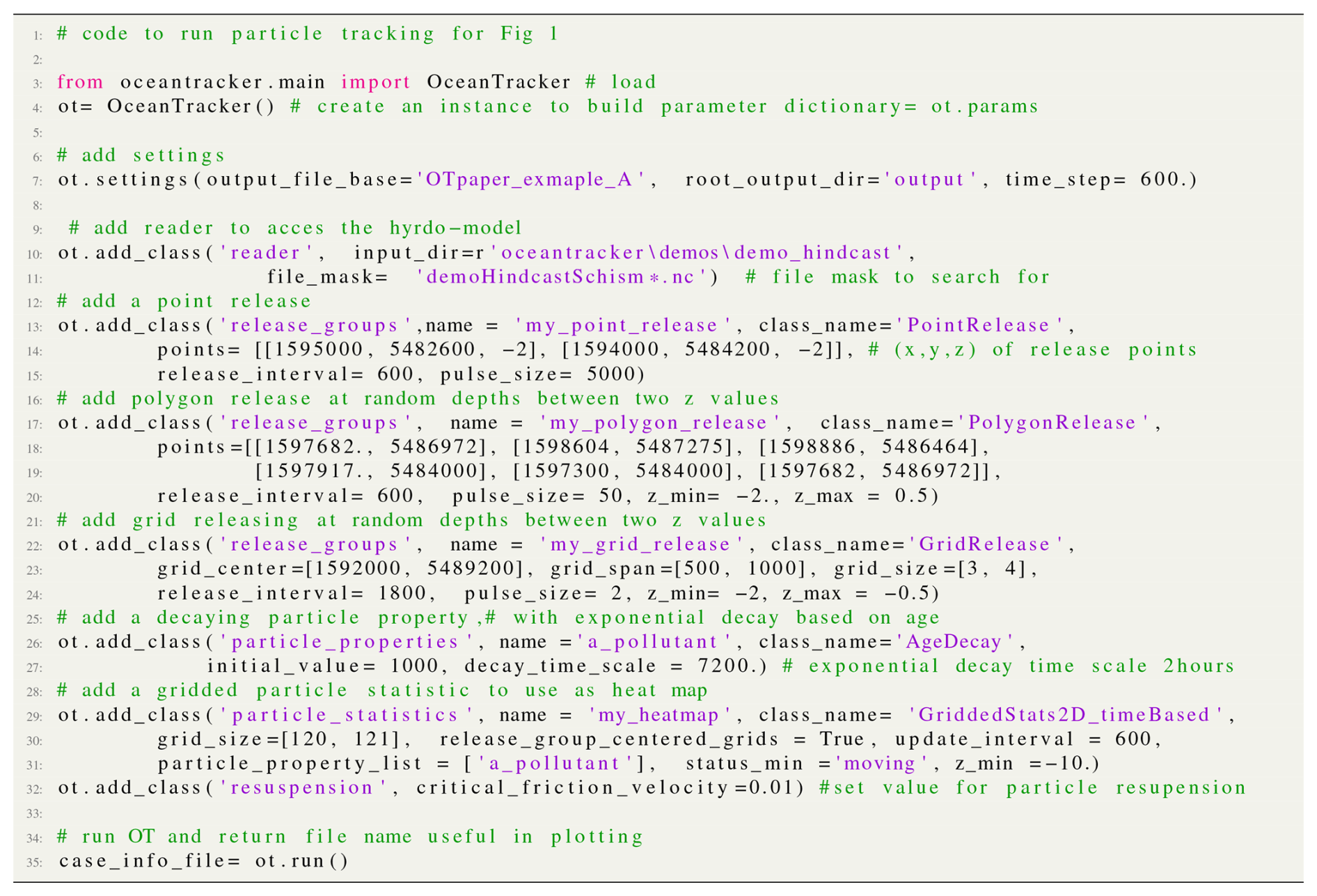
Figure 1 Examples of results from point, polygon and grid particle release groups computed during a single run, Sect. 4.5. Plots give results at the end of a 4 d run. In the upper figures, the crosses in the upper left are the locations of a grid particle release, while the black polygon is the area covered by a polygon release. The crosses near the middle of the plots are locations of two point releases. (a) A snapshot of the particles: blue indicates particles that are moving and green particles those that are stranded by an outgoing tide. Dry cells are shown in brown, and blue shading indicates water depth. (b) Particles are sized and coloured according to a decaying particle property, see Sect. 4.2.2. (c) Heat map of log particle counts with each grid cell from a release of 5.7 million particles from a pair of point sources. (d) Heat map of decaying particle property on a logarithmic scale. The region shown is part of Tasman Bay (located at the northern end of New Zealand's South Island) and part of a hydrodynamic model of Cook Strait used in Atalah et al. (2022). The heat maps in the lower plots are based on a user specified regular grid with a 100 m resolution. The code to run this example is provided in Appendix A (Fig. A1).

2 Example

Figure 1 presents basic examples of OceanTracker outputs from a 3D simulation, with particles released from points, polygons and a regular grid, all within the same computational run, see Sect. 4.5. The snapshot in Fig. 1a displays particles coloured according to their status, moving (blue) or stranded by the tide (green). For the upper two plots in Fig. 1, the two points each released 5 particles every 10 min, the polygon released 50 particles every 10 min and the grid released 2 particles every 3 h at depths between 2 and 0.5 m below sea-level datum. A total of 35 000 particles were released over the 4 d run. Figure 1 presents results at the end of the run.

Heat maps can be used to illustrate the decay and dispersion of a pollutant from its source. OceanTracker creates heat maps on the fly, by counting particles that fall within cells of a user-specified regular grid overlaid on the hydrodynamic model grid during trajectory computation. OceanTracker's efficiency may enable particles counts large enough, such that sufficient numbers fall within each grid cell to create visually smooth heat maps.

The two points in the lower plots of Fig. 1 each released 5000 particles every 10 min, giving 5.7 million particles by the end of the 4 d run. This resulted in an average of 500 particles being counted within each grid cell to create the heat maps. This appears sufficient to give a smooth heat map for a 100 m resolution user specified grid. Creating this heat map bypassed the need to record large volumes of particle trajectories (see gridded statistics in Sect. 4.8 and code in Appendix A). Figure 1d illustrates a heat map of the average value of a user-added exponentially decaying particle property.

3 OceanTracker – new features

This section highlights some of the new features of OceanTracker v0.5 that minimise user effort and its physics.

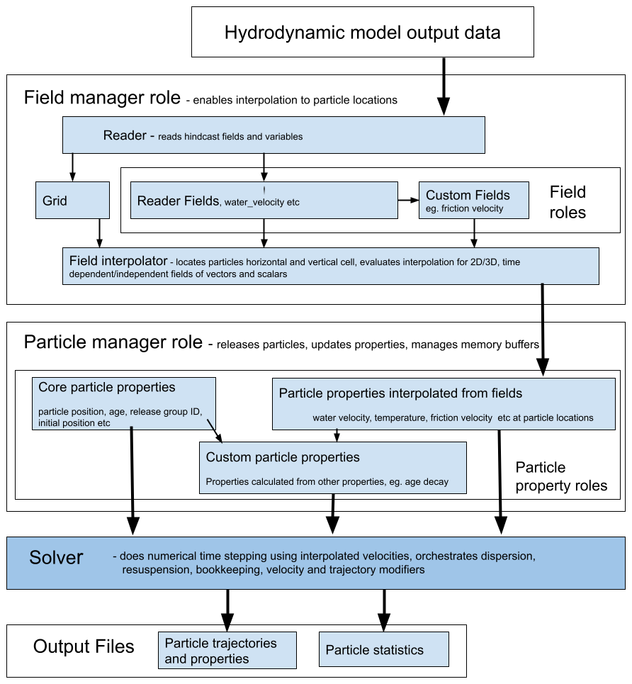
Figure 2 Outline of the data flow through the two main data structures, fields and particle properties, from hydrodynamic model files to output. These data structure roles are outlined in Sect. 4.2. Each has “managers” to orchestrate operations on the variants of each data structure, to deliver particle properties to the solver. The steps carried out by the solver are shown in Fig. 3.

3.1 Features reducing user effort

In addition to computational speed, OceanTracker incorporates a number of features that significantly reduce the time and effort required to obtain results from the analysis of particle trajectories. The most significant features are:

• Release groups. Simultaneous release of multiple groups of particles can be done, each with distinct locations and timing. This functionality enables users to obtain multiple results from a single computational run (see Fig. 1, Sect. 4.5 and Appendix A). This may eliminate the need for setting up and managing multiple runs to explore different release scenarios.

• On-the-fly particle statistics. OceanTracker enables the simultaneous computation of multiple statistics while calculating trajectories, reducing post-processing effort. For instance, within the same run OceanTracker can generate heat maps for moving and settled particles while also calculating the connectivity between different areas defined by polygons, all within the same trajectory computational run . These statistics are based on counting particles within user-specified grids or polygons as trajectories are calculated. These “on-the-fly” statistics are calculated separately for each release group, e.g. individual heat maps for each release site, or connectivities between releases within multiple polygons and another set of polygons.

• Coding productivity. User written custom components can be added to OceanTracker by class inheritance using the widely used Python language and NumPy package (Harris et al., 2020). In addition, computationally intensive tasks can often be accelerated by simply adding a Numba decorator to their functions that use Python and NumPy code (Lam et al., 2015). This bypasses the need to learn an additional language, such as C, to computationally speed intensive operations (more on Numba in Sect. 5).

• Self-managing particle buffer. Particle properties such as current location or status are stored in memory buffers, that expand dynamically as more particles are released. This removes the need to specify the maximum number of particles that will be used in advance. Memory buffers are also dynamically consolidated as particles are killed to minimise the total memory required, allowing efficient computation within limited memory.

3.2 Physics features

Along with advection by water velocity, the core physics features that affect particle motions are outlined below. A coding user can easily adapt these to create required variants through class inheritance.

• Dispersion. A random walk mechanism simulates dispersion due to sub-hydrodynamic grid-scale processes as a first order Markov process (Lynch et al., 2014; Van Sebille et al., 2018). As in the earlier version of OceanTracker, random walk can be incorporated using constant turbulent eddy viscosities in both the horizontal and vertical directions. Optionally in the new version, if vertical turbulent viscosity profiles are available in a 3D hydrodynamic model, the profiles are interpolated to calculate the size of the vertical random walk. This requires the inclusion of an additional vertical velocity that is equal to the vertical gradient of the turbulent viscosity (Visser, 1998; Thorpe, 2005). Note that the random walk is not applied as a step change in position but as an equivalent additional velocity. This dispersion velocity modifier is calculated once for each full time step and added to the hydrodynamic model's velocity at each Runge-Kutta (RK) sub-step, see Fig. 3 and Sect. 4.6.

• Re-suspension. Particles that settle on the seabed can be re-suspended if the flow is strong enough. The likelihood and height of re-suspension depends on the friction velocity (Lynch et al., 2014, their Eq. 9.28). Stronger flows increase the probability of re-suspension and cause particles to be lifted higher into the water column. The friction velocity is calculated from the near-bed velocity using a logarithmic velocity profile or, if available, from the bottom-stress field in the hydrodynamic model output (Lynch et al., 2014, their Eqs. 5.5 and 5.6).

• Tidal stranding. Particles within hydrodynamic model cells that become dry as the tide recedes remain stationary until the cell becomes wet again. Dry cells are “flagged” based on flags in the hydrodynamic model files. If a dry cell flag is not available, a cell is considered dry when the total water depth at its centre falls below a user-specified minimum value.

• Backtracking. OceanTracker supports reverse-time simulations, which can be useful for identifying potential sources of particles arriving at a given location (Thygesen, 2011). Note that dispersion is not time-reversible, and this operates the same in the forward-direction time, producing outputs, like heat maps, that offer a probabilistic view of sources (Thygesen, 2011).

• Nested grids. To enable particle tracking beyond the open boundaries of a single hydrodynamic grid, OceanTracker can nest multiple inner grids within a broader, coarser outer grid. Particles exiting the open boundary of an inner grid are transferred to the outer grid, and particles on the outer grid which move inside an inner grid, are transferred to that grid. Each particle is aware of its current grid, allowing field values to be interpolated from the relevant grid. The inner and outer grids may consist of any combination of structured or unstructured grids.

Beyond these core physical processes, OceanTracker allows users to optionally add particle behaviour by adding additional bio-physical processes, e.g. Atalah et al. (2022). This is achieved by adding given components to specific computational roles, such as velocity modifiers (e.g., sinking velocities) and trajectory modifiers (e.g., particle splitting or larval behaviours), as described in Sect. 4.7 and 4.6.

4 OceanTracker structure

At a high level, particle tracking code takes the Eulerian water velocity field from a hydrodynamic model and interpolates these to provide velocities at particle locations. These velocities are then numerically integrated to give particle trajectories. There are also multiple other processes and computations that must be done at each time step, including the physical processes of dispersion, resuspension and tidal stranding. OceanTracker decomposes these processes into a series of components that fulfil specific roles, which are part of the computational pipeline outlined in Fig. 3 and Sect. 4.

Figure 2 illustrates the data flow in OceanTracker from hydrodynamic model files through to outputs via its two main data structures: fields and particle properties (see Sect. 4.2). Fields store data from the hydrodynamic model, such as water velocity, salinity and wind stress, as well as custom fields that are calculated from other fields, such as friction velocity. Particle proprieties hold data for each particle, which could include their current location, status or temperature. These data structures enable access to, and operations on, their data, and they are collectively “managed” by their respective manager roles (see Sect. 4.3).

4.1 Computational pipeline

The computational pipeline is constructed from components assigned to specific roles within the pipeline that implement required tasks at each time step (Fig. 3). From a user's perspective, the adaptability of OceanTracker comes from the ability to customise which components are added to each role to create a computational pipeline to meet their specific needs. For example, a gridded 2D statistic can be added to the “particle statistics” role to create heat maps of particle locations on-the-fly.

These components are constructed as Python classes, which are dynamically added to the computational pipeline during setup. Time stepping within the computational pipeline proceeds by calling the “update” method of each component within each role. Some roles, such as dispersion and re-suspension, allow only one class to be added, while others allow the addition of multiple classes. For example, multiple trajectory modifiers can be combined to give the required particle behaviour.

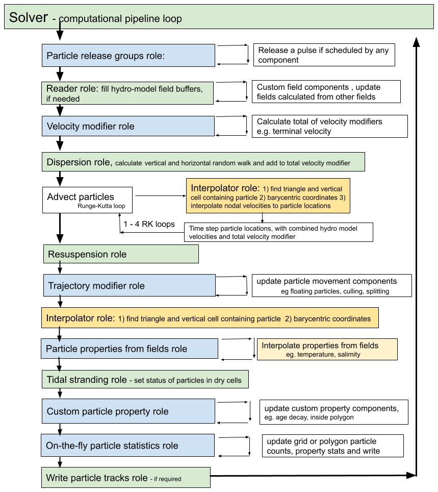
Figure 3 Flow chart of time stepping to advect particles within the solver component in Fig. 2. The figure illustrates the order in which components are updated within their roles in the computational pipeline. These operation roles are outlined in Sect. 4.2. Green “core roles” only contain one component. Blue roles may contain one or more components that are looped through. For large runs, the most computational expensive steps are (1) finding the cell containing each particle and (2) evaluating the field interpolation; these steps are coloured yellow.

4.1.1 Building a computational pipeline

The computational pipeline in OceanTracker can be fully assembled at startup from parameters provided in either a JSON or YMAL text file or a Python dictionary, eliminating the need for direct coding if using only inbuilt components (see Fig. 4b, c). Alternatively, for simulations that add many classes (eg. hundreds of different release groups), coders can add their parameters programmatically within loops, using helper wrapper methods. This wrapper provides two key methods “settings” and “add_class” which enable users to construct a parameter dictionary using keyword arguments (see Fig. 4a). The resulting parameter dictionary follows the same structure as the JSON text file format shown in Fig. 4c and is passed to OceanTracker for execution.

Users can configure top-level settings, such as the particle tracking time step and output directories, as well as component-specific settings. This trajectory calculation process constitutes a series of roles performed by a collection of components. Each component’s configuration typically includes the name of the Python class assigned to a particular role. Most component settings have default values defined within their respective Python classes, but some class settings must be explicitly provided by the user. During setup, all user-defined settings are automatically validated for type correctness and appropriate value ranges. To run OceanTracker a user must add at least a reader class and one release group class. In addition, they must set the name of the folder where output will be written to (see Fig. 4a).

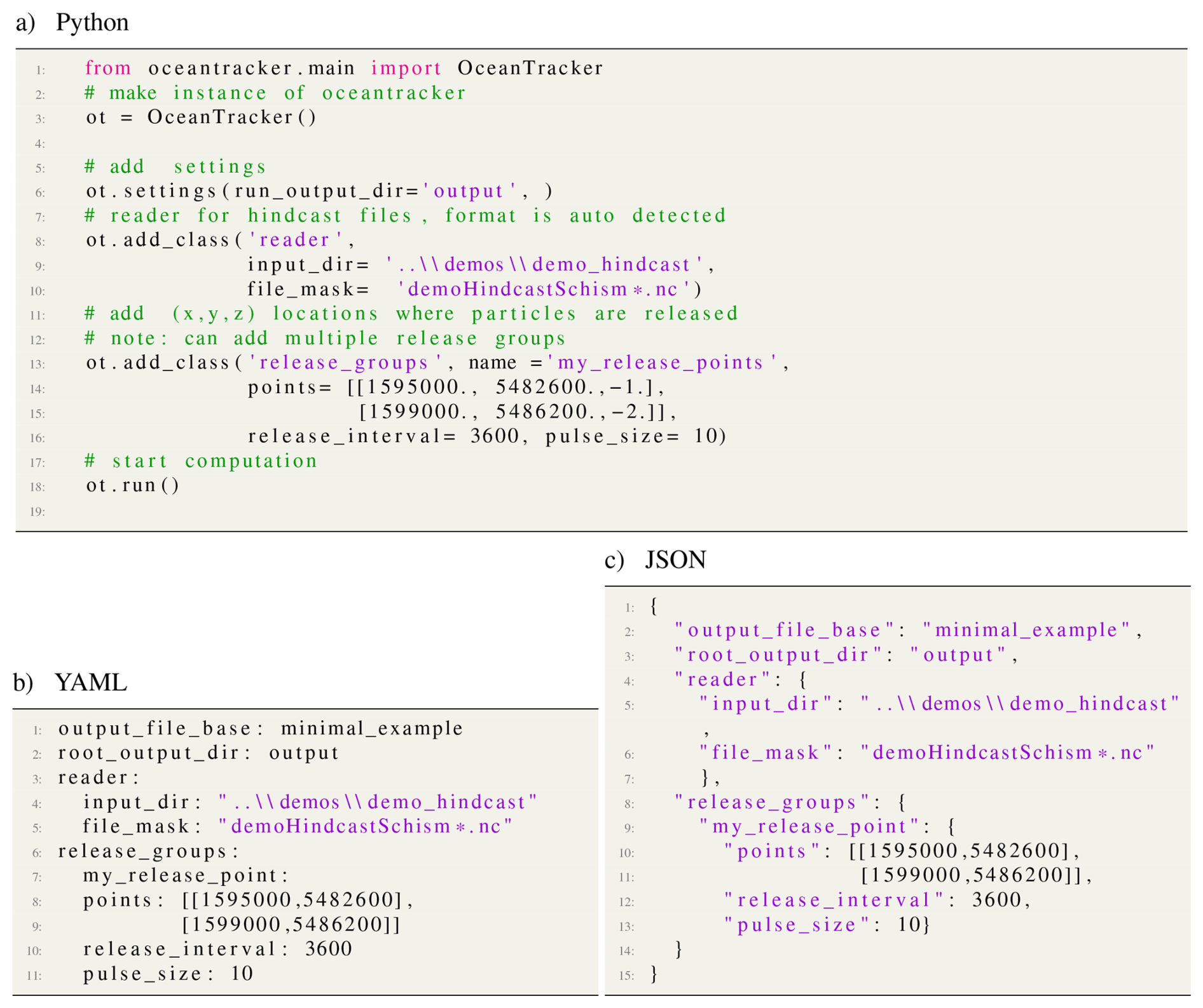
Figure 4 Minimal example of building a computational pipeline (a) by coding, using “helper” wrapper methods “settings” and “add_class” methods to set up parameters and run code. A computational pipeline can also be built from a text file with user supplied parameters in either (b) YAML or (c) JSON standard formats.

4.1.2 Computational steps

Time stepping in OceanTracker integrates particle velocity to compute trajectories. Within the computational pipeline, time stepping is divided into a series of roles, each performed by one or more components, see Fig. 3. The update of each component is automated within the time stepping of the computational pipeline, with updates grouped by role, see Fig. 3. The order in which the roles are updated reflects their temporal dependence on the data from other roles. For example, custom particle properties may be calculated from field particle properties and are therefore updated after the interpolated field properties. The solver class implements the time stepping by managing the classes within the computational pipeline and the associated bookkeeping functions.

The first step in the computational pipeline involves looping over the release groups and releasing a single pulse containing a user specified number of particles, if scheduled for the current time step. After this, each newly released particle's current horizontal and vertical cell are calculated. The solver then checks if the reader field time buffers contain the required time steps; if not, the reader fills the buffers and any custom fields are calculated from the newly read time steps. Next, any additional particle velocities are added together to give a total of “velocity modifiers” (e.g. a fall velocity) and to this total a random walk dispersion is added as an equivalent velocity, see Sect. 3.2. Particles are then advected by RK integration based on the sum of the water velocity and the total of the velocity modifiers. At each sub-step, their current horizontal and vertical cells and barycentric coordinates are updated, enabling each particle's velocity to be interpolated to their locations. By default, fourth order RK time integration is used, although first and second order RK are also available.

Once particles are at their new locations, additional changes to particle status or positions due to resuspension or specified trajectory modifiers are made. These modifiers add any additional particle movements or changes to their status, e.g. settling in a polygon or culling. To enable interpolation after these movements, particle horizontal and vertical cells and barycentric coordinates are updated. Then, all field-derived particle properties are then looped over and updated by interpolation. Subsequent steps include updating any custom particle properties, calculating any particle statistics that have been added to the computational pipeline, and then finally writing out time series of particle trajectories and particle properties if this has been requested.

4.1.3 Mechanisms enabling computational pipeline adaptability

The following mechanisms provide the flexibility needed to build the computational pipeline dynamically at run time and enable coders to extend OceanTracker:

• Dynamic importing. Components for all roles are dynamically imported at runtime, allowing users to build custom computational pipelines. To specify a component, users provide a “class name” setting (see Sect. 4.1.1), which follows standard Python class referencing conventions. Core roles have default class names, and all built-in OceanTracker classes can be imported using a shortened version of their full names. Users can also import customised variants of Python classes into any of the roles in the computational pipeline, enabling them to modify core functionality or add optional functionality (e.g. dispersion models, trajectory modifiers or on-the-fly statistics).

• Inheritance. New component variants can be created by inheriting from an existing class. Users can modify computations by overwriting specific methods, such as the “update” method, while retaining inherited configuration settings and the infrastructure than manages bookkeeping operations. This approach allows for incremental modifications of the parent class.

• Internal naming. To simplify access to the main data structures outlined in Fig. 2 OceanTracker uses standardised names for instances of the field and particle property components. These instances are held in globally accessible field and particle property Python dictionaries. Additionally, both reader-sourced and custom user-defined fields automatically generate particle properties of the same name, by interpolation at each time step. Essential fields like “water velocity” and “water depth” are mapped to corresponding variable names in the hydrodynamic model files by the reader component. Vector fields may require mapping multiple file variables to a single internal name. Users can also assign names to optional components for easier reference within their output files and code.

4.2 Data structures within the computational pipeline

This section outlines OceanTracker's two main data structures, fields and particle properties, see Fig. 2, while Sect. 4.3 describes their management.

4.2.1 Field role

The spatial fields stored within the output of the hydrodynamic model are the foundation of offline particle tracking and are stored and accessed using the “field” data structure, see Fig. 2. Water velocity is a crucial spatial field for particle tracking, but there may be many other relevant fields, such as water depth, tide or wind-stress. There are also grid variables associated with the fields, including nodal locations, triangulation and cell adjacency. These are also accessed through a map that links their name in the hydrodynamic model output to standard internal names.

Fields are read from hydrodynamic model files as described in Sect. 4.4. Users can also integrate custom fields into the computational pipeline by deriving new values from existing fields. For example, a friction velocity field can be computed from the 3D velocity field near the seabed to determine whether a particle can be re-suspended by the flow.

4.2.2 Particle property role

There are three types of particle properties that store the values for each particle and enable high level operations on these values as shown in Fig. 2b. These properties can have different types depending on how they are updated at each time step, and they may be integer, scalars or vectors.

• Field particle properties store field values at each particle location and are updated by interpolating a field data structure, e.g. water velocity.

• Core particle properties are updated within the core code, i.e. not by their own class update method. Examples include particle location and bookkeeping particle properties, such as particle ID, release group ID, or particle status, e.g. whether computationally alive, on the sea bed, stranded by the tide etc.

• Custom particle properties store values calculated from other particle properties. For example, the “inside-polygons” class uses the location particle property to determine whether any user-given polygon contains each particle. These are updated by calling their classes's update method.

Some examples of currently available custom particle properties are:

• Age decay models an exponentially decaying particle load, such as bacteria, based on the core “age” particle property

• Inside polygon records the polygons, from a given set that contain a particle. This information is used to compute polygon connectivity statistics or to determine events such as larval settlement when a particle drifts over a reef.

• Total water depth represents the sum of tidal elevation and water depth. This property is useful for particles whose behaviour differs in varying water depths, such as larvae that only settle in shallow water, even if a cell is not completely dry.

4.3 Manager roles

Instances of field and particle properties store, update, and manage access to individual data values. Higher level operations on all the individual instances are orchestrated by “managers” that automate key processes (see Fig. 2).

• Fields group manager role. Orchestrates the setup, reading, updating and interpolation of fields, along with setting up the required grid variables, such as nodal locations, triangulation and the adjacency matrix. It also manages the process of finding each particle's current horizontal and vertical cell, and updates the status of dry cells. By default, the fields group manager automatically adds a particle property with the same internal name as the field to the computational pipeline, which are interpolated at each time step. When nesting small fine-scale grids within a larger outer grid, a special master fields group manager orchestrates a set of field group managers, each associated with a hydrodynamic model grid. It associates each particle with the appropriate grid, so that the water velocity and other particle properties can be interpolated from the fields of that grid. At each time step, any particles crossing the open boundaries of the inner grid are associated with the outer grid. Conversely, any particles on the outer grid that move inside an inner grid are then associated with that grid.

• Particle group manager role. Manages the release of particles and the updating of all three types of particle properties. It also manages the dynamic memory buffers that hold the individual particle property values, expanding them as needed when particle numbers grow and also culls computationally dead particles that are no longer of interest. Additionally, if required, this manager handles the writing of time series of particle trajectories and properties.

4.4 Reader role

The primary function of the reader is to convert hydrodynamic model file variables, which may be stored in different files, into standardised internal formats. The reader builds a catalogue of all file variables and which files contain them. From this catalogue, the reader identifies if the hydrodynamic output is a known format and imports the associated reader class. It identifies known formats by looking for a set of expected signature variables within the files. The file variables are then mapped to standard internal variable names. Field variables are categorised as time varying, vector or 3D. The reader does this by determining if each variable's named dimensions contains dimensions associated with these attributes for the known hydrodynamic model. For vector variables, e.g. water velocity, several file variable names can be mapped to a single internal vector variable, allowing vector fields to be treated as a single variable within computations.

To ensure files for time-varying variables are read in the correct order, files are sorted into time order, using the hydrodynamic model's time variable. Thus OceanTracker is not reliant on a file naming convention to determine file order. Each variable has its own list of files, which enables the reader to accommodate hydrodynamic models where variables are split between files, as is the case for SCHISM version 5 output files and NEMO/GLORYS output files.

The reader loads fields into memory buffers as they are needed. For time-dependent variables it reads multiple time steps into buffers, if the next time step is not already in the buffer. By default, the buffer maintains 24 hydrodynamic model time steps in memory. This default number of steps balances reducing wall time, by reading in multiple time steps at the same time, while only requiring of 100s of megabytes of computer RAM for each buffered hindcast variable. The user can reduce this buffer size if RAM is limited.

If needed, the reader converts the non-nodal values to values at the nodes of the triangles through interpolation. Readers and interpolators that are based on a hydrodynamic model's native grid and do not need this conversion, could be developed in the future. To facilitate automation, the reader stores all fields in 4D arrays with dimensions (corresponding to time, node, depth layer and vector components).

The unstructured SCHISM and DEFLT3D-FM grids contain a mixture of triangular and quad cells. For these formats and regular grid formats, quad cells are divided into triangles. This division simply takes the first three nodes of a quad cell as one triangle, then creates a new triangle from the third, fourth and first nodes. Modifying the “triangulation” of the hydrodynamic model grid by splitting quad cells is only done once at the start of the run and it has no impact on the time spent reading the hindcast. It also adds little to the memory used, as the underlying field values are still stored as nodal values. By increasing the number of cells to search, quad cell splitting may sightly increase the time taken to locate the cell containing each particle. However, it simplifies the code by only requiring one type of cell to search.

4.4.1 Interpolator role

The interpolator serves as the link between the hydrodynamic model's fields held by the reader and the corresponding particle properties. The interpolator has two functions: (1) determining each particle's current horizontal and vertical cell; and (2) interpolating field values at the triangles' vertices to each particle's location, which are then stored as particle properties. In the horizontal, OceanTracker currently uses linear interpolation in unstructured triangular grids from nodal values, utilizing a particle's Barycentric coordinates within their current triangle, along with linear interpolation between hydrodynamic model time steps.

Vertical interpolation to the position of each particle is also linear between the layers of the hydrodynamic model and between time steps. The one exception to linear vertical interpolation is the water velocity within the seabed layer. Here, vertical interpolation is based on a logarithmic layer, ensuring that particles near the seabed experience a more realistic velocity profile than the linear variation in higher layers Lynch et al. (2014).

The interpolator supports linear interpolation for several vertical grids, Sigma grid (ROMS, Deft-3D FM) and fixed z levels (Deft-3D FM, NEMO/GLORYS), which apply the same vertical grid at all locations. It also supports grids with spatially varying layer thicknesses (SCHISM, FVCOM). This includes SCHISM's LSC vertical grid, where the number of vertical layers also varies spatially.

4.5 Particle release groups role

A “particle release group” introduces new particles into the computational pipeline. Each group generates new particles at specified locations, which are released at user set intervals or times with a specified number per release, or “pulse size”. Multiple release groups can be added, each with their specific release locations, release schedules or pulse size. Release groups can be:

• Point release. Particles are spawned from a set of specified locations and depths, such as the two crosses in the middle of the plots in Fig. 1. A radius release class, releases particles randomly within a circular area around each point.

• Polygon release. Particles are spawned at random locations within a user-defined 2D polygon, e.g. mid-right of the upper plots in Fig. 1.

• Grid release. Particles are spawned from points of a user specified regular grid, as on the upper left of the upper plots in Fig.  1.

Particles will not be released on land, e.g. where a release polygon overlaps land as in Fig. 1a. By default, particles are not released within cells that are currently dry due to the outgoing tide. For all types it is possible to restrict releases so that they are randomly distributed within a given vertical layer, at fixed distance from seabed or sea surface or to locations where water depth is within a given range.

4.6 Velocity modifiers role

Additional bio-physical processes can be added to the water velocity experienced by each particle. These are incorporated into the computational pipeline as “velocity modifiers”, which are added to the water velocity for use in the time integration, see Fig. 3. Terminal velocity is an example of an in-built modifier that adds the terminal sinking or buoyant velocity to the ambient water velocity, either as a uniform value or a particle specific value drawn from a normal distribution.

4.7 Trajectory modifiers role

Components in the “trajectory modifiers” role implement bio-physical processes that alter the status or movement of particles at each time step. Examples of inbuilt modifiers include:

• Settlement allows particles to settle within user defined polygons, e.g. larvae to settle on reefs. The trajectory is modified by changing its status to “stationary”.

• Floating sets each particle's vertical position to that of the free-surface height at its current location.

• Culling sets the status of a random fraction of particles for a given status (e.g. on the bottom) to be dead, allowing them to be removed from subsequent computations and particle statistics.

• Splitting splits particles in two to simulate e.g. reproduction, at a set rate or probability. This can rapidly generate very large numbers of particles, which may need to be contained by a culling mechanism (Steidle and Vennell, 2023).

4.8 On-the-fly particle statistics roles

OceanTracker employs an on-the-fly particle counting approach to produce particle statistics during the computational run. This produces a data output volume that is independent of the total number of released particles. Currently available spatial particle statistics are:

• Gridded counts particles inside the cells of a regular grid at user-specified time intervals. These are commonly used to generate heat maps (see Fig. 1).

• Polygon computes the physical connectivity matrix between each release group and user-defined polygonal regions.

Both gridded and polygon-based statistics can be recorded using two approaches:

• Time series counts particles at specified time intervals, producing time-based heat maps or connectivity data.

• Age bin series categorises particles into age bins within each spatial region, enabling the generation of age-based heat maps or connectivity matrices.

Users can filter which particles are counted, for example they can restrict statistics to particles within a specific vertical range or to particles resting on the seabed. Multiple on-the-fly statistics components can be added, which allows, for example, separate particle counts for different depth layers.

Beyond counting particles, average values of particle properties can also be computed within the spatial bins. For instance, users can track average water temperature of particles within a given grid cell or polygon.

4.9 Integrated models

Users may need to combine multiple roles to create higher level functionality. OceanTracker supports this aggregation of roles into a single component, enabling sharing of specialised combined functionality amongst users. These integrated models only require the parameters essential for executing their higher-level function; the model manages the intricacies of assigning classes to appropriate roles to complete the overall function. Currently, there is one integrated model:

• On-the-fly Lagrangian Coherent Structures. These structures identify regions of convergence or divergence within a fluid flow over time. OceanTracker calculates time series of Finite-Time Lyapunov Exponents (FTLE) (Haller, 2015; Harrison and Glatzmaier, 2012), which can be used to derive characteristics of Lagrangian Coherent Structures. The FTLE calculation uses the largest Eigenvalue of the strain tensor after specified lag times. This process involves releasing particles on a regular grid and calculating the distances between adjacent released particles. The user only needs to designate one or more grid locations and the required time lags. The integrated model sets up new regular grid releases at regular time intervals and calculates the FTLE on-the-fly for each grid and lag, eliminating the need to record and post process large volumes of particle trajectories.

5 Computational speed

The primary features contributing to OceanTracker's computational speed measured by wall time are:

• Finding cells containing particles. For unstructured grids, significant computational time is spent determining the horizontal and vertical cells containing each particle. OceanTracker uses the particle history to improve the speed of its cell search. Short triangle and vertical walk algorithms improve the search speed by an order of magnitude compared to long triangle walks or KDE tree approaches, as outlined in Vennell et al. (2021).

• Calculate once, use many times. To avoid repetition in performing key computational tasks, a particle's current triangle, barycentric coordinates, vertical cell and fraction of the vertical cell are recorded at each time step. These values are then used repeatedly to interpolate multiple fields to the particle's location. Adopting the “calculate once, use many times” methodology significantly improves the efficiency of interpolations (Vennell et al., 2021).

• Dynamic particle buffer. Particle proprieties are stored in memory buffers, which are expanded as needed to accommodate newly released particles. System performance and memory utilisation can be optimised by periodically culling dead particles, e.g. those too old to be of interest. When more than 25 % are flagged as dead, particle memory buffers are compacted by removing the dead particles, which can significantly improve performance.

• Uniform sigma grid. For 3D SCHSIM and FVCOM models layer thicknesses vary temporally and spatially, making the search for each particle's vertical cell the most time-consuming step. Optionally, for these models, the vertical cell search can be made 5 times faster by vertically linearly interpolating to spatially uniform sigma-layer fractional thicknesses when filling the reader's buffers. With uniform fractional thicknesses, finding the vertical cell is significantly quicker using rounding within a pre-calculated layer map, followed by a single correction step. For large numbers of particles, the time spent re-interpolating to this near-native vertical grid when reading the hydrodynamic model's files, is small compared to the time saved by the faster vertical cell search. Models that use a sigma vertical grid can directly exploit a faster approach to the vertical cell search with no additional effort. Though vertical interpolation means particle motions are not strictly a result of velocities of the native hydrodynamic model grid, but rather an approximation of those velocities.

• Numba. Particle tracking involves complex operations with nested loops, requiring per-particle decisions at each time step. To significantly accelerate these computations, OceanTracker leverages Numba, a Python extension for Just-In-Time (JIT) compilation (Lam et al., 2015). Numba optimises performance by compiling functions at runtime using a simple function decorator. Numba achieves execution speeds comparable to C or Cython while maintaining Python’s ease of use. Once a function is compiled, the optimised code is reused for subsequent calls, eliminating further compilation overhead. However, a drawback of using Numba is that compiling the many required functions adds 20–30 s to OceanTracker's startup time. This delay can be minimised by enabling optional caching, which stores the compiled Numba code on disk for reuse between runs.

• Field storage precision. Hydrodynamic models typically store field values as 32 or 64 bit floating point numbers. However, 64 bit floats require twice the memory of 32 bit floats. More importantly, these fields must be transfered from computer RAM to CPU registers before they are used to calculate interpolated values. This transfer may limit the speeds at which computations can be done. To reduce transfer time, OceanTracker stores all hydrodynamic model fields at 32 bit floats, regardless of how they are recorded by the hydrodyamic model.

• Parallelisation. OceanTracker spreads most demanding computations across all available physical computer cores, exploiting Numba's multithreading capabilities. Specifically, when iterating over particles OceanTracker uses Numba's parallel for-loop, to automatically distribute particle computations across multiple physical cores. All threads access the same field variable memory; thus each hydrodynamic model time step is only read once during the run. This makes OceanTracker suitable for running on a single computer or single node of a super-computer where cores share the same memory.

5.1 Input/Output speed

The speed at which the hydrodynamic model can be read may contribute significantly to total run times. The times in Table 1 are based on reading from local disks. Reading model data from internet sources would be expected to be slower. In the Table 1 examples, the proportion of read time varies from 36 % for basic Laptop I to 50 % for high end Desktop II. These values are for 1 million particles, larger numbers would dilute these read times. For particle numbers where 50 % or more of time is spent reading the hydrodynamic model on a user's hardware, the number of particles could be doubled to obtain better statistics, while only increasing wall time by 25 %.

For large numbers of particles, the time spent writing particle tracks can also add significantly to run times; particularly as writing tacks is typically a serial process, whereas trajectory computations can be parallelised. The times in Table 1 do not include the time to write tracks. This potentially significant time was part of the reason behind developing on-the-fly statistics, as this eliminates the necessity to write particle tracks for subsequent analysis.

5.2 Speed comparisons

The computational performance of OceanTracker (version 0.5.1.1) and its closest alternative OpenDrift (version 1.11.1) (Dagestad et al., 2018) are compared in Fig. 6 for structured and unstructured grids. A similar comparison has been reported in Vennell et al. (2021). The base code has since undergone a significant overhaul, from using NumPy and SciPy for critical computational steps to using Numba. This transition has facilitated the implementation of far more particle-specific decision processes that enhance the realism of their movement. A speed comparison with Parcels (version 3.0.6) (Delandmeter and Van Sebille, 2019) is also included in Fig. 6. Both Parcels and OceanTracker can exploit parallelisation, with Parcels using processing via MPI, while OceanTracker uses multithreading via Numba. OpenDrift does not natively support parallelisation but can be used to run multiple independent cases, each separately reading the hydrodynamic model, an approach referred to as “embarrassingly parallel”. Thus, the comparisons presented here show performance using only a single process and thread to provide comparable results across the three models. Parcels currently only supports structured grids, so could only be compared with OceanTracker for this type of grid.

All comparisons use 3D hydro-dynamic models. The first is a high-resolution unstructured mesh estuarine model described in Steidle and Vennell (2023), built using SCHISM (Zhang et al., 2016). This model features 32 000 horizontal nodes and employs terrain-following coordinates for the vertical grid, with up to 20 levels. Its spatial resolution varies from 5 to 1400 m. The second model is a regular grid ROMS model presented in López et al. (2020), consisting of about 250 000 nodes and 40 z-grid type vertical levels with a uniform horizontal resolution of 7 km. The third model is a large NEMO/GLORYS model of the Baltic Sea (Kärnä et al., 2021), which contains about 600 000 horizontal nodes and 56 z^*-grid type vertical levels. All hydrodynamic models had a temporal resolution of 1 h.

OceanTracker and OpenDrift were compared using dispersion, while the comparison to Parcels using the NEMO data set were performed using advection only, due to a lack of a native 3D dispersion method in Parcels. For Parcels the “JITParticle” class was used as the advection kernel. All particle trackers used 4th order Runge-Kutta (RK4) time integration. The computations covered 10 model days using 5 min time steps, resulting in a total of 2880 time steps. Particles were released at 30 locations, with total particle numbers varying from 1000 to 1 million particles per model run. Note that OpenDrift by default uses a different time step size for its vertical diffusion calculations of 1 min. We chose not to override this default behaviour as OpenDrift's internal timing information shows that the computational cost did not dominate the total runtime (<10 %) and is similar to what we expect based on our experience with OceanTracker.

The computational experiments were performed on the desktop computer “imf20-l01”, which was equipped with an Intel(R) Core(TM) i5-10500 CPU @ 3.10 GHz and 16 GB RAM. The relative performace of OceanTracker and the other two codes may differ on other hardware. The source code that has been used to perform this speed tests is publicly available (see Code and data availability).

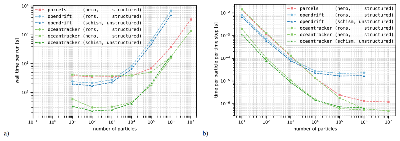
Figure 5 Computational comparison speed for OceanTracker with OpenDrift for structured (ROMS) and unstructured (SCHISM) grids, and with Parcels for structured (NEMO/GLORYS) grids. (a) Comparison of the total run time measured as wall time. (b) Normalized computational time per particle per RK4 time step.

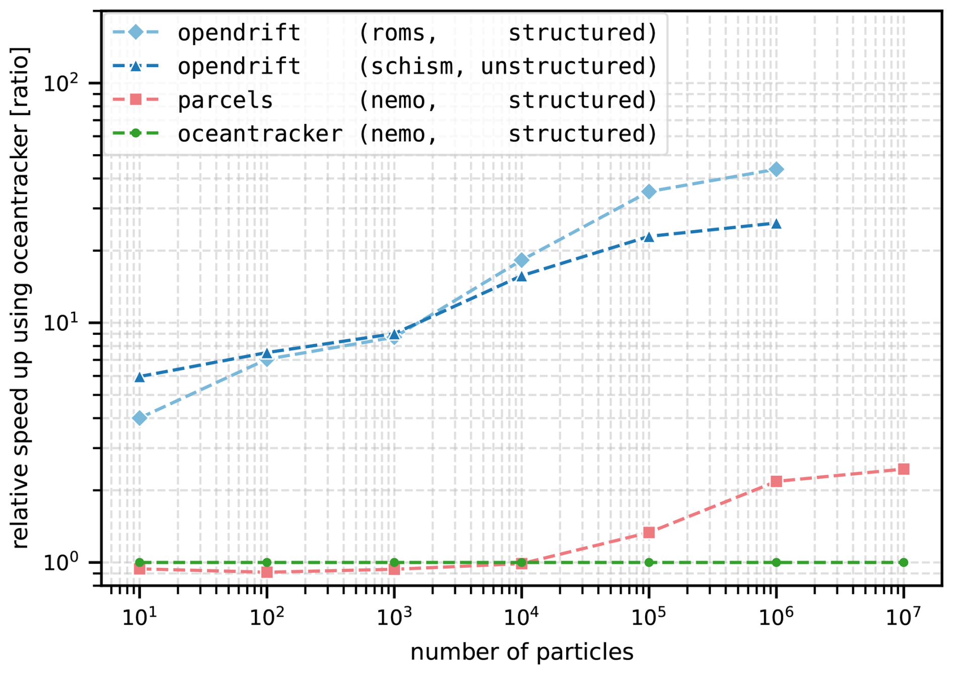
Figure 6 Comparison of the relative speed up from OceanTracker compared to OpenDrift and Parcels for the different data sets and particle sizes. The green line represents the baseline performance equal to OceanTracker.

Figure 5a displays the total run time across OceanTracker and OpenDrift (structured and unstructured grids) and Parcels (structured grid). Figure 5b illustrates the scaling of both models in terms of time per particle per RK4 time step. This demonstrates that OceanTracker can process around a million particles per second per time step on a single desktop core.

For the SCHISM and ROMS data set, model setup times are the main contributor to OceanTracker's run time for particle counts up to 10 000. For these small numbers, OpenDrift's minimum run time was approximately 2 min, while OceanTracker's completed these runs in 30 s. For particle counts exceeding 10 000 setup times become negligible for both models. In 1 million particle simulations OceanTracker is up to 35 times faster than OpenDrift as shown in Fig. 6, resulting in total run times of 15 h for OpenDrift and 30 min for OceanTracker.

OceanTracker treats structured grids as unstructured grids by triangulating them, whereas OpenDrift uses a native reader for the structured ROMS grids. Surprisingly, the native ROMs reader of OpenDrift does not significantly enhance its performance with structured grids.

For the NEMO/GLORYS case, which uses a large data set with over 3 million spatial nodes, model setup times and reading the data remains the dominant cost for cases with particle counts of below 100 000. For larger particle counts over 1 million, OceanTracker performs approximately twice as fast as Parcels. To our knowledge, this demonstates that OceanTracker is the fastest general-purpose particle tracker for both structured and unstructured grids.

5.3 Multi-core scaling

OceanTracker utilises use Numba's multi-threading capability for parallelisation across mutiple cores. Figure 7 shows the multi-threading scaling for two machines (note the logarithmic x-axis). The first is the high-performance computer “Levante” based at the DKRZ (German Climate Computing Center). It is equipped with two AMD 7763 CPUs @ 2.45–3.5 GHz, containing 128 physical cores in total and 256 GB of RAM. The second is “imf20-l01”, a desktop computer that was also used for the single thread speed tests. Scaling quickly becomes sub-linear for threads counts greater than two, presumably due to bandwidth limitations between the CPU memory caches and the much larger Random Access Memory (RAM) when accessing particle or hindcast data. This bottleneck becomes strongly limiting on Levante for thread counts above 32, with no improvements between 64 and 128 threads. The latter is expected because multi-threading is limited to only one of the two available physical CPUs. This data access bottleneck indicated the need to improve how speed scales with the number of threads. This could be achieved by restructuring the code to slice up the hydrodynamic hindcast into sub-domains distributed across threads, or by redesigning how particle data is ordered in memory (Kehl et al., 2023).

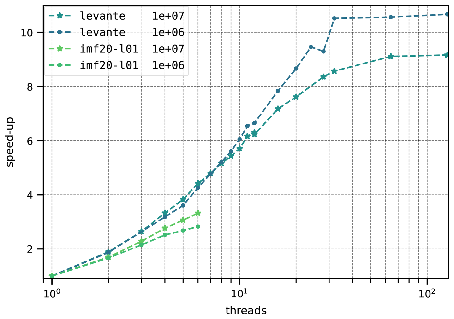
Figure 7 Scaling of computation speed when run in parallel mode. The vertical axis is the speed-up relative to single thread runs. Comparisons were performed on “imf20-l01”, a standard office desktop machine, and on node of Levante, a high-performance computer, with 128 CPU cores for particle counts of 1 and 10 million (1×10⁶ and 1×10⁷). Note the logarithmic scaling on the x-axis.

6 Discussion

Vennell et al. (2021) found that OceanTracker performs significantly faster than OpenDrift when working with unstructured grids. Here, Fig. 5 demonstrates that the new version of OceanTracker maintains a speed advantage on structured grids, despite treating them as unstructured. This result is somewhat surprising since, as cell identification is typically much faster in structured grids because it only requires rounding coordinates. The observed performance difference suggests that the advantage is not due to differences in cell-finding algorithms, but rather other aspects of how the two models handle computations. Note that for the speed comparisons we focused exclusively on computational time as our metric. Because all models internally show significant difference in their implementations it was not possible to configure them to perform the exact same computation. Hence, for future comparisons it would be desirable to compare computational cost while normalising for model accuracy.

For unstructured grids, the original OceanTracker was over two orders of magnitude faster than OpenDrift (Vennell et al., 2021). The latest version of OceanTracker is an order of magnitude slower than its predecessor. However, this trade-off comes with significantly improved physics, see Sect. 3.2. The enhancements require more computationally intensive, particle-by-particle decisions regarding movement. While these decisions introduce slower branching code, they result in more realistic particle behaviour and improved simulation accuracy.

To validate OceanTracker's accuracy, we performed a standard test using a circular flow with a known period, as recommended by Van Sebille et al. (2018). A 2D synthetic eddy test was conducted, featuring a peak flow of 1 m s⁻¹ at a 10 km radius with a 12 h period. With 15 min RK4 time steps, particles released 10 km from the centre deviated by less than 0.3 m from their initial radius after 10 d, demonstrating high accuracy.

6.1 Design compromises

The design of OceanTracker makes a number of compromises between speed, steepness of the adoption curve, adaptability and the complexity of its implementation code. Though speed was high priority, in a number of places other aspects had higher priority. The below outlines some of OceanTracker's design compromises.

• Class modularity vs speed. The computational pipeline in Fig. 3 is a series of steps, where an operation needs to be completed for all particles, before moving on to the next operation. This approach moves all particles one operation at a time along the computational pipeline. A downside of this approach is that the same particle property data may be moved between RAM and CPU for several times per time step, slowing code, i.e becomes memory-bound. An alternative is to complete all operations of the computational pipeline for each particle, before moving on to the next particle. When compared to the modular approach, this could significantly increase overall speed by reducing the volume of intermediate results that must be transferred between RAM and CPU. The disadvantage of performing all operations on each particle is it limits flexibility, making it more difficult to dynamically add or modify components within the pipeline. It may also require users to have a high level of coding ability to adapt the computational pipeline to their needs. Thus, the memory-bound modular approach of OceanTracker compromises speed while significantly enhancing adaptability, particularly for novice users. Adapting OceanTracker for GPUs may lead to faster performance due to their better memory access speeds.

• Automation vs code complexity. OceanTracker's design abstracts the computational pipeline into a series of roles, within which individual components carry out the functions requested by the user. This allows aspects of the pipeline to be automated, e.g. auto detection of hydrodynamic model type and required fields, where particle properties are automatically interpolated from named fields, and written to output files. While, this internal automation helps deskill the computational pipeline for the user, it adds significantly to the internal complexity of OceanTracker's code. This heavily relies on modularity based on class inheritance to implement the abstracted pipeline, in order to accommodate many user options and multiple hydrodynamic model formats. As a result parts of OceanTracker's code may be harder to develop.

• Abstraction limitations. The modular computational pipeline abstraction in Fig. 3 could limit the types of problems that OceanTracker can be used to solve. For example, the effects of trajectory modifiers and velocity modifiers are added to each other. However, there are be examples where this linear superposition of effects approach may not be able to implement users requirements. For example if the magnitude of several velocity modifiers each depend on the combined total of the water velocity and all velocity modifiers.

7 Summary

OceanTracker v0.5 provides a comprehensive ocean particle tracking framework compatible with both structured and unstructured grids. Its computational speed allows users to scale to larger numbers of particles on modest computer hardware within acceptable run times. Simulating larger numbers facilitates enhanced particle statistics and broader exploration of variations in particle behaviours. Integrating the calculation of particle statistics directly within computational runs may significantly reduce the time required to derive statistics. In addition, on-the-fly-statistics produce more manageable data volumes, as their size does not depend on the number of particles released. The ability to add multiple release groups and statistics also reduces user efforts, by enabling multiple outcomes within the same computational run. Adaptability in building a computational pipeline is enabled by a modular approach to roles within the pipeline. Moving OceanTracker to a full version 1.0 release will require additional development. For example, more testing is needed to ensure compatibility with a wider range of variants of the currently supported hydrodynamic model formats, as well as adding support for other popular model formats. In addition, more comprehensive documentation, users guide and tutorials that will help make the adoption curve less steep.

OceanTracker's computational speed primarily stems from its algorithmic efficiency in locating each particle’s current triangle and interpolating field values at its position. This efficiency allows it to significantly outperform current versions of OpenDrift and Parcels on a single computer core. When using more than 30 cores, OceanTracker's performance increases by an additional factor, further surpassing models that do not leverage parallel computation.

For small particle counts, reading the hydrodynamic model data will dominate the run time, making the actual trajectory calculations negligibly short. For the Laptop I and Desktop II benchmarks in Table 1, the tipping point between time spent reading and time spent calculating trajectories is around 100 000 and 1 000 000 particles respectively. Trajectory computation for significantly smaller particle numbers is almost free. This tipping point will be higher for hydrodynamic models with more nodes or a larger particle tracking time step than those used for the examples in Table 1.

Future improvements to enhance OceanTracker's computational speed might include greater use of “Single Instruction Multiple Data instructions” on conventional CPUs (Kehl et al., 2023). Additional optimisation may be possible by adapting expensive computational kernels to take advantage of GPUs. Speed could may also be improved by chunking or restructuring the data in memory (Kehl et al., 2023). An asynchronous reader could fill field buffers in a separate parallel process and share memory with the particle computational threads. This could make reading the hydrodynamic model almost “free” in terms of overall run times for numbers above the tipping point, or the trajectory computations free for numbers below this point.

Appendix A: Code for Fig. 1

Figure A1 Python code used to run the particle tracking example shown in Fig. 1.