Automated stratigraphic interpretation from drillhole lithological descriptions with uncertainty quantification: litho2strat 1.0

Australian commonwealth, state and territory geological surveys possess information on over 3 million drillhole logs. In addition to mineral exploration drilling, extensive drillhole datasets exist from oil and gas exploration and hydrogeological studies. Other countries no doubt have similar data holdings. Together these legacy drillhole datasets have the potential to significantly enhance constraints on regional 3D geological models and improve our understanding of subsurface architecture, but have limited use in their current form as many if not most drill logs lack stratigraphic information, containing only lithological descriptions.

This study develops open-source codes and methodologies for stratigraphy recovery (determining the ordered sequence of stratigraphic units) from drillhole lithological data by introducing a search algorithm that systematically explores all geologically plausible stratigraphic orderings for individual drillholes, combined with a solution correlation algorithm that compares the topological relationships of stratigraphic units across multiple drillholes to identify geologically consistent solutions and reduce uncertainty. The algorithms combine constraints from lithological descriptions with stratigraphic relationships automatically derived from regional maps. In addition, the method quantifies uncertainty by generating multiple plausible stratigraphic interpretations, providing critical insights for resource estimation, scenario analysis, and data acquisition strategies.

The application of our method to a dataset of 52 drillholes from South Australia demonstrated its ability to make useful predictions of stratigraphic solutions and quantifying associated uncertainties. These results not only validate our approach but also highlight opportunities to refine current stratigraphic descriptions and provide a valuable new source for regional 3D geological modelling.

1 Introduction

Drillhole data serve as a fundamental constraint for subsurface geological exploration and 3D geological modelling, offering direct insights into lithological and hence stratigraphic features (Wellmann and Caumon, 2018). However, the inherent sparsity of such data, coupled with challenges posed by legacy datasets maintained by industry and Geological Survey Organizations (GSOs), often hinders comprehensive geological understanding and modelling (Jessell et al., 2010; Pakyuz-Charrier et al., 2018). GSOs' databases typically contain lithological information as unstructured text descriptions (e.g., “sandy limestone with minor shale”) but rarely include stratigraphic unit assignments. This creates a critical gap in the data needed for accurate and meaningful geological predictions (Hartmann and Moosdorf, 2012).

Geological modelling plays a crucial role in understanding subsurface structures and processes, providing a foundation for various applications in earth sciences (Jessell et al., 2014). Such modelling commonly relies on datasets such as borehole data, geophysical data, and mapping data. Among these, borehole data provide the most accurate insights into subsurface geology and stratigraphy (Guo et al., 2022). The models generated through geological modelling can serve dual purposes: they can be directly employed for geological interpretations, such as identifying fault systems and mineral deposits (Alvarado-Neves et al., 2024; Vollgger et al., 2015), or they can be integrated as constraints in methodologies that use a prior 3D model, such as geophysical inversions (Giraud et al., 2017; Martin et al., 2024; Ogarko et al., 2021; Tarantola, 2005) and hydrogeological forward modelling (D'Affonseca et al., 2020).

Modern drillhole measurement techniques primarily focus on chemical, mineralogical and lithological characterization, whereas the fundamental categorical unit of regional 3D geological models is defined by stratigraphy (Calcagno et al., 2008; Caumon et al., 2009; Mallet, 2002). This discrepancy underscores the need for innovative approaches to recover and integrate stratigraphic information from existing datasets.

Recent advancements in automation have made significant progress in processing drillhole data, though most address different aspects of the problem than stratigraphic recovery. Data standardization tools like dh2loop (Joshi et al., 2021) extract and harmonize lithological descriptions from unstructured text using thesauri and fuzzy string matching, providing essential preprocessing for downstream analysis. Pattern recognition methods (Schetselaar and Lemieux, 2012) can identify lithostratigraphic markers and contacts within drill logs, helping to detect boundaries between units. Machine learning approaches for 3D geological modeling (Guo et al., 2024) can interpolate between drillholes to create subsurface models, but typically require pre-interpreted stratigraphic data as input. While these methods provide valuable components of the workflow, none directly address the fundamental challenge of transforming lithological descriptions into stratigraphic interpretations with quantified uncertainties.

Existing automated interpretation methods primarily work with different data types than those available in legacy drillhole databases. Geophysics-based methods (Wu and Nyland, 1987; Fullagar et al., 2004; Silversides et al., 2015) leverage distinctive signatures in gamma, resistivity, or other wireline logs to predict stratigraphic units, but require geophysical data that are absent from most legacy drillholes. Geochemical and spectral approaches (Hill and Uvarova, 2018; Hill et al., 2021) use XRF scanning or hyperspectral measurements to identify geological boundaries with high precision, but depend on expensive data acquisition unavailable in historical datasets. Hybrid machine learning methods, such as those applied in the Pilbara iron ore deposits (Wedge et al., 2019), combine lithology with assays and geophysics but require extensive pre-interpreted drillhole datasets for training, limiting their application in greenfield exploration areas. These approaches do not address the fundamental challenge faced by geological surveys worldwide: millions of legacy drillholes contain only lithological descriptions but lack both stratigraphic interpretations and the geophysical logs required by current automated methods.

To address these challenges, we formulate the problem of stratigraphic recovery from drillhole databases as follows. The input to our methodology consists of: (1) legacy drillhole databases containing lithological descriptions (e.g., “sandstone”, “siltstone”, “dolomite”) at various depth intervals, typically without stratigraphic labels; (2) regional geological maps that define stratigraphic unit boundaries and their spatial relationships; and (3) topological constraints that specify which stratigraphic units can be in contact based on their known relative ages and depositional sequences. The output comprises: (1) multiple plausible stratigraphic solutions, where each solution provides unit assignments for all depth intervals in the drillholes; (2) their ranking by geological likelihood; and (3) quantified uncertainties for these interpretations. The objective is threefold: first, to systematically transform lithological descriptions into stratigraphic interpretations by testing all geologically plausible orderings of stratigraphic units that are consistent with the observed lithologies; second, to quantify the uncertainty inherent in these interpretations given that multiple stratigraphic units may share similar lithological characteristics; and third, to establish correlations between multiple drillholes to reduce uncertainty and improve the reliability of stratigraphic assignments across a region. This transformation is essential because regional 3D geological models are fundamentally organized by stratigraphy rather than lithology, yet the majority of legacy drillhole data lack stratigraphic labels.

Figure 1 illustrates this challenge with a simplified example: a drillhole log with four lithological intervals (sandstone, siltstone, sandstone, dolomite) could correspond to multiple stratigraphic interpretations. The two sandstone intervals might represent the same formation repeated by faulting, or they could belong to different formations with similar but distinct lithological compositions. Without additional constraints, both interpretations are geologically plausible, highlighting the inherent ambiguity in stratigraphic assignment from lithological data alone.

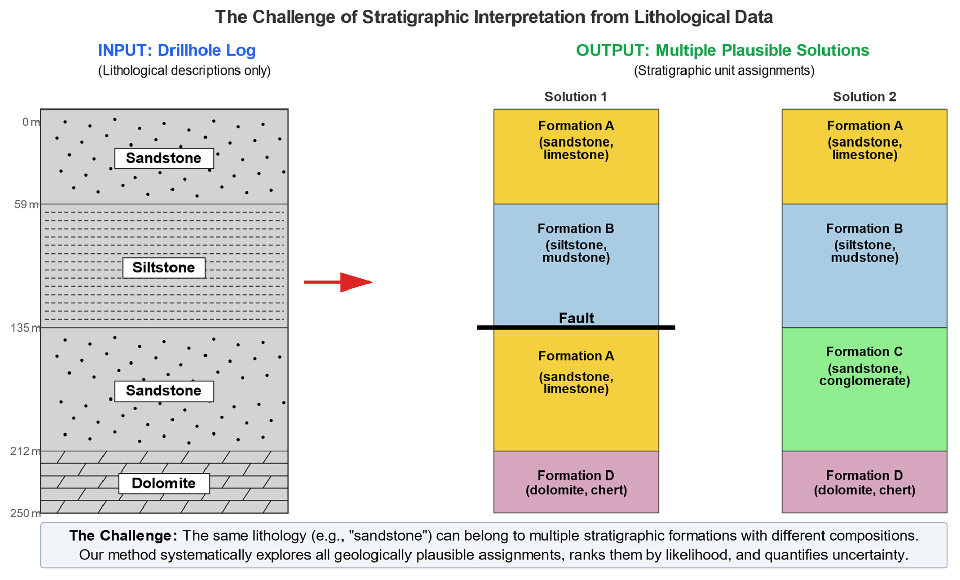
Figure 1 Schematic illustration of the stratigraphic interpretation problem. A drillhole log containing only lithological descriptions (left) can yield multiple plausible stratigraphic solutions (right) because the same lithology may occur in different stratigraphic formations with varying compositions.

This study develops open-source codes and methodologies for stratigraphy recovery from drillhole lithological data through a two-stage approach. First, we introduce a branch-and-prune search algorithm that systematically explores all geologically plausible stratigraphic orderings for individual drillholes. Second, we apply a solution correlation algorithm that integrates information from multiple drillholes by comparing topological relationships of stratigraphic units, thereby enhancing the robustness and reliability of interpretations. The method quantifies uncertainty by generating multiple plausible stratigraphic interpretations, providing critical insights for resource estimation, scenario analysis, and data acquisition strategies. We apply our method to a dataset of 52 drillholes from South Australia to demonstrate its practical application and validate its performance against existing stratigraphic interpretations.

2 Methodology

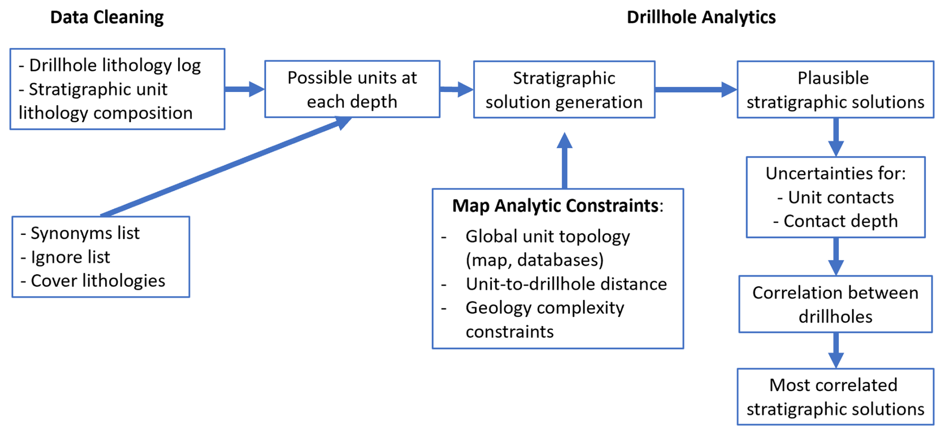
2.1 Workflow

The workflow shown in Fig. 2 consists of three key steps grouped into three main tasks: Data Cleaning (using the dh2loop code), Map Analytic Constraints (using map2model and custom codes developed for this project) and Drillhole Analytics (using the litho2strat code developed for this project).

Figure 2 The different stages of the analysis.

2.1.1 Data Cleaning

Prior to analysing the drillhole data we went through a number of automated data cleaning and harmonisation steps.

• a.

  Harmonisation of drillhole lithology descriptions using the dh2loop code described in Joshi et al. (2021) (code available here: https://github.com/Loop3D/dh2loop, last access: 27 January 2026) This enables us to produce a standardised lithological description for multiple drillholes in a region, regardless of their provenance. This includes the use of a synonym list (“granite” vs “granitoid”), and ignore list (e.g. “fault”) together with a list of cover lithology terms (e.g. “saprolite”) that enables us to simplify the list of terms and exclude irrelevant information.

• b.

  Harmonisation of lithological descriptions for formations described in the geological map of the target area. This ensures that the same terminology is used for borehole lithological descriptions and map lithologies.

Together steps a and b ensure consistent lithological terminology across drillhole logs and geological map units, enabling subsequent stratigraphic unit matching (Sect. 2.2).

2.1.2 Map Analytic Constraints

• a.

  Calculation of the distance between each polygon in a map and the target borehole. A custom Python script was developed. This information can be used as a guide to the likelihood that a drillhole would intersect a given unit.

• b.

  We then used the map2model engine (Jessell et al., 2021) (code available here: https://github.com/Loop3D/map2model_cpp, last access: 27 January 2026) to extract the topological relationships between the surface expression of stratigraphic different units. This would later be used to assess the likelihood that two units would be in contact in the drillhole.

The map2model engine extracts topological relationships between stratigraphic units, including both normal depositional contacts and fault contacts, as both types of juxtaposition may be encountered in drillhole data.

Unit connectivity information can also be obtained from the Australian Stratigraphic Units Database (ASUD) as well as from various published reports containing stratigraphic data (Geoscience Australia and Australian Stratigraphy Commission, 2017). The ASUD serves as a comprehensive repository of geological information, providing valuable insights into the relationships between different stratigraphic units across Australia. Additionally, numerous geological surveys and research studies offer stratigraphic data that can further enrich our understanding of unit connectivity. Leveraging this information, enhances stratigraphic models, improves the accuracy of correlations between drillholes, and facilitates a deeper understanding of the geological framework in specific regions.

These two steps allow us to capture information on the spatial and topological relationships between the mapped units.

2.1.3 Drillhole Analytics

In this stage, we employ the litho2strat code to generate plausible stratigraphic solutions that fit the observed lithological data while satisfying all geological constraints (code available here: https://github.com/Loop3D/litho2strat, last access: 27 January 2026; Ogarko and Jessell, 2025). The algorithm uses a recursive branch and prune approach to efficiently explore the solution space, eliminating geologically implausible pathways early in the search process (see Sect. 2.2 for detailed algorithm description). This strategy not only ensures thorough exploration of viable stratigraphic orderings but also optimizes computational efficiency by avoiding unnecessary enumeration of invalid solutions.

From the complete ensemble of plausible solutions obtained for each drillhole, we calculate uncertainties that quantify the confidence in different stratigraphic interpretations. Solutions are scored based on the probability of unit contacts within the local solution ensemble, providing a ranking of stratigraphic hypotheses from most to least likely.

To further reduce uncertainty and improve solution reliability, we implement a correlation algorithm that leverages information from multiple neighboring drillholes simultaneously (see Sect. 2.5 for correlation algorithm details). By comparing the topological relationships of stratigraphic units across drillholes, the correlation process identifies solutions that are geologically consistent across the broader area. Correlated solution scores integrate both local evidence from individual drillholes and regional consistency with neighboring holes, with solutions receiving the highest correlated scores selected as the most plausible stratigraphic interpretations.

2.2 Stratigraphic solution generation

The litho2strat algorithm operates through a hierarchical search strategy that systematically explores the space of possible stratigraphic orderings (solutions) while pruning geologically implausible solutions. The algorithm can be formally described as follows:

Input:

• $L=\mathit{\{}{l}_{\mathrm{1}},l_{\mathrm{2}},\mathrm{\dots },l_n\mathit{\}}$: sequence of n lithologies observed at depths $d_{\mathrm{1}}<d_{\mathrm{2}}<\mathrm{\dots }<d_n$

• $U=\mathit{\{}{u}_{\mathrm{1}},u_{\mathrm{2}},\mathrm{\dots },u_m\mathit{\}}$: set of m candidate stratigraphic units, each defined by its constituent lithologies

• C: set of geological constraints (distance, connectivity, complexity)

• Γ: global unit connectivity graph derived from geological maps and stratigraphic databases

Output:

• $S=\mathit{\{}{s}_{\mathrm{1}},s_{\mathrm{2}},\mathrm{\dots },s_k\mathit{\}}$: set of k plausible stratigraphic solutions

• P(s_i): probability distribution over solutions

• G_h: local connectivity graph for drillhole h, derived from all solutions for this drillhole

Algorithm Steps:

1. Unit Matching Phase. For each lithology l_i at depth d_i, identify the subset of compatible units:

   $$\begin{array}{}\text{(1)}& \begin{array}{rl}M\left(l_i\right)& =\mathit{\{}{u}_j\in U:\mathrm{lithology}\left(u_j\right)\mathrm{matches}{l}_i\\ & \text{AND satisfies constraints}C\mathit{\}}\end{array}\end{array}$$

2. Recursive Branch and Prune Exploration. The algorithm recursively builds the solution space from shallow to deep depth intervals. Starting from the surface, partial solutions are extended one depth level at a time by considering candidate units that match the observed lithology. The algorithm generates a new branch for candidate unit u_j only when all of the following conditions are satisfied:

   • –

     The unit u_j matches the observed lithology at the current depth

   • –

     The extended solution satisfies all constraints in C (distance, occurrence, contact complexity)

   • –

     For the last unit u_k in the partial solution, the edge (u_k,u_j) exists in the global connectivity graph Γ

   Partial solutions that violate any condition are immediately abandoned (pruned), preventing exploration of their extensions. When a partial solution reaches the deepest depth interval, it is validated and added to the solution set S. This recursive approach with constraint-based pruning eliminates large portions of the solution space without explicit enumeration.

   The algorithm systematically explores all geologically valid solutions through exhaustive search with constraint-based pruning. While the top-to-bottom traversal order does not affect the completeness of the final solution set S (the same valid stratigraphic interpretations would be found regardless of traversal direction), it does improve computational efficiency by enabling earlier application of surface geology constraints and more effective pruning of invalid solution branches.

3. Local Connectivity Graph Construction. From the complete set of solutions S obtained for drillhole h, construct a local connectivity graph G_h where edge weights represent the frequency of unit contacts across all solutions:

   $$\begin{array}{}\text{(2)}& w_h\left(u_j,u_k\right)={\displaystyle \frac{\left|\mathit{\{}s\in S:\text{contact}\left(u_j,u_k\right)\text{exists in }s\mathit{\}}\right|}{\left|S\right|}}\end{array}$$

   This directed local graph captures the probability of unit contacts based on the ensemble of geologically plausible solutions for drillhole h, where edges represent stratigraphic ordering. Each edge weight represents the fraction of solutions in which the corresponding unit contact appears. Note that G_h is a subgraph of the global connectivity graph Γ, as all solutions for drillhole h must satisfy the global connectivity constraints.

4. Solution Scoring. For each solution s_i ∈ S, calculate a normalized score based on the local connectivity graph G_h:

   $$\begin{array}{}\text{(3)}& \mathrm{score}\left(s_i\right)={\displaystyle \frac{{\sum }_j{w}_h\left(u_j,u_{j+\mathrm{1}}\right)}{N_i}}\end{array}$$

   where N_i is the number of unit contacts in solution s_i (i.e., $N_i=\left|s_i\right|-\mathrm{1}$), and the sum is over all consecutive unit pairs. The normalization by N_i ensures that solutions with different numbers of stratigraphic contacts are directly comparable, preventing bias toward longer or more complex solutions. The score thus represents the average edge probability across all contacts in the solution.

5. Probability Calculation. Normalize scores to obtain probability distribution:

   $$\begin{array}{}\text{(4)}& P\left(s_i\right)={\displaystyle \frac{\mathrm{score}\left(s_i\right)}{{\sum }_k\mathrm{score}\left(s_k\right)}}\end{array}$$

   The efficiency of this approach derives from constraint-based pruning during the recursive exploration. By evaluating both solution constraints C and global connectivity Γ before extending each partial solution, the algorithm eliminates inconsistent paths immediately without exploring their complete extensions. The distinction between the global connectivity graph Γ (used for constraint validation during exploration) and the local connectivity graph G_h (derived from solutions and used for scoring) is crucial: Γ represents a priori geological knowledge from maps and databases, while G_h captures the a posteriori probability distribution of unit contacts specific to drillhole h given all constraints.

2.3 Solution constraints

For the Branch and Prune algorithm described in Sect. 2.2, providing efficient constraints (collectively denoted as C) is crucial for generating geologically plausible stratigraphies and reducing the search space. Without these constraints, the algorithm would need to exhaustively enumerate all possible unit assignments, which is computationally prohibitive. We utilize two types of solution constraints: the first can be derived from geological maps (as discussed in the “Map Analytic Constraints” section), while the second is selected by the user based on the expected structural complexity of the area (e.g., the presence of faults, folds, or other features that might cause stratigraphic repetition or disruption).

The specific constraints in C include:

1. Distance Constraint. This constraint limits the number of geological units considered based on their proximity to the drillhole. In this context this is defined as the distance between the drillhole collar and the nearest point on the polygon's boundary in 2D. For drillhole h and candidate unit u_j ∈ U:

   $$\begin{array}{}\text{(5)}& d\left(u_j,h\right)\le d_{max}\end{array}$$

   where d(u_j,h) is the distance from the nearest outcrop of unit u_j to drillhole h, and d_max is the maximum search radius. This ensures relevance to the drillhole's location.

2. Global Unit Connectivity Constraint. This constraint, enforced through the global connectivity graph Γ, restricts potential contacts between units. For any two consecutive units u_j and u_j+1 in a solution:

   $$\begin{array}{}\text{(6)}& \left(u_j,u_{j+\mathrm{1}}\right)\in E\left(\mathrm{\Gamma }\right)\end{array}$$

   where E(Γ) is the edge set of the global connectivity graph. This ensures that only units known to be stratigraphically adjacent (from map data, databases, or published reports) can be placed in contact, enhancing the geological plausibility of solutions.

   The edges in the global connectivity graph Γ can be configured as either single-directional or bidirectional depending on the structural complexity of the study area. In structurally simple areas with normal stratigraphic succession, single-directional edges (e.g., A→B) enforce the expected younging direction (older to younger upward). However, for areas with known structural complexities such as overturned sequences from folding or thrust faulting, bidirectional edges can be used to allow stratigraphic contacts in both normal and reversed orientations. For example, if units A and B can occur in both normal succession (A overlies B) and overturned succession (B overlies A) due to folding, the graph Γ would include a bidirectional edge between them, allowing transitions in both directions (A→B and B→A). This configuration allows the algorithm to exhaustively explore all structurally valid solutions including those with reversed polarity sequences. The choice of single-directional versus bidirectional edges in Γ is thus a key input that controls whether the algorithm considers only normal superposition or also accommodates structural inversions.

3. Top Unit Constraint. Information regarding the top unit u_top can be extracted from geological maps at the surface location of the drillhole, providing a foundational boundary condition:

   $$\begin{array}{}\text{(7)}& s\left[\mathrm{0}\right]=u_{\mathrm{top}}\end{array}$$

   where s[0] denotes the shallowest unit in solution s. Note that while the global unit connectivity constraint allows sequences to begin from any node in the connectivity graph, this constraint explicitly specifies the starting node.

4. Occurrence Constraint. This constraint sets a maximum limit on how many times a unit can appear in a solution, accounting for geological complexity such as faulting or folding. For unit u_j in solution s_i:

   $$\begin{array}{}\text{(8)}& \mathrm{count}\left(u_j,s_i\right)\le k_{max}\end{array}$$

   where count(u_j,s_i) is the number of times unit u_j appears in s_i. Typically $k_{max}=\mathrm{1}$ for unfaulted sequences, or $k_{max}=\mathrm{2}$–3 for faulted terrains where stratigraphic repetition may occur.

5. Contact Complexity Constraint. For a continuous sequence of identical lithology observations [$l_i,l_{i+\mathrm{1}},\mathrm{\dots },l_{i+m}$] where all lithologies are the same, this constraint limits the number of distinct stratigraphic units that can be assigned:

   $$\begin{array}{}\text{(9)}& \left|\mathit{\{}{u}_j:\text{assigned to interval\hspace{0.17em} }\left[i,i+m\right]\mathit{\}}\right|\le c_{max}\end{array}$$

   where c_max is the maximum number of unit contacts allowed within the continuous lithology sequence. This prevents over-interpretation where a thick monotonous lithology (e.g., a 100 m sandstone sequence) is artificially divided into an excessive number of stratigraphic units.

6. Stratigraphic Jump Constraint. To account for incomplete exposure of geological contacts at the surface, we relax the map-based connectivity constraint by allowing the algorithm to “jump” over intermediate units in the global connectivity graph Γ. For a path in Γ such as $A\to B\to C$, setting the maximum number of stratigraphic jumps parameter to j_max allows direct contacts between non-adjacent units up to jmax steps apart in the graph. For example, with $j_{max}=\mathrm{1}$, the algorithm can consider both A→B and A→C as valid contacts, even if A→C is not explicitly observed in the map data. This addresses the limitation that geological maps provide only a 2D surface expression of 3D geological relationships and may not capture all possible stratigraphic contacts that exist at depth.The constraint is enforced by permitting contacts between units u_i and u_j if:

   $$\begin{array}{}\text{(10)}& d\mathrm{\Gamma }\left(u_i,u_j\right)\le j_{max}+\mathrm{1}\end{array}$$

   where dΓ(u_i, u_j) is the shortest path distance between units u_i and u_j in the connectivity graph Γ, and j_max is the maximum number of allowed jumps (typically $j_{max}=\mathrm{0}$ for strict adherence to observed contacts, or $j_{max}=\mathrm{1}$–2 for more permissive exploration).

   These constraints in C work together to enhance the efficiency and effectiveness of the Branch and Prune algorithm, ensuring that the resulting stratigraphies are both geologically plausible and computationally tractable. As demonstrated in Sect. 3, constraint-based pruning reduces the search space by > 99 % in practical applications.

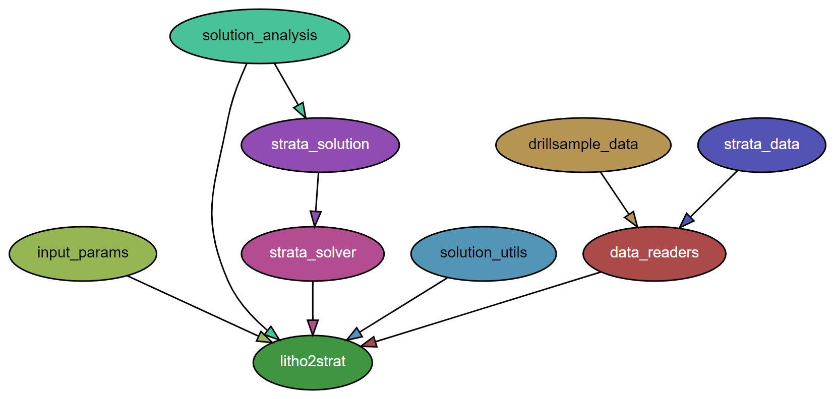
Figure 3 The module dependencies of the litho2strat code. The graph is generated by the pydeps utility, while excluding external dependencies.

2.4 Computational complexity

The computational complexity of the branch and prune algorithm depends on several key factors: the number of drillholes H, the length of the lithology sequence $\left|L\right|$ (i.e., the number of depth intervals), the number of candidate stratigraphic units $\left|U\right|$, and critically, the average number of solutions N maintained during the recursive exploration. The algorithm processes each drillhole independently, and for each drillhole, it iterates through all lithologies in L, evaluating potential unit assignments for each active solution.

The theoretical time complexity can be expressed as:

$$\begin{array}{}\text{(11)}& O\left(H\times \left|L\right|\times N\times \left|U\right|\right)\end{array}$$

where N denotes the average number of solutions maintained during recursive exploration. This is the most variable factor and depends strongly on the geological complexity and the constraints applied.

In the unconstrained case, where no geological constraints are imposed, the number of solutions can grow exponentially with the number of lithology changes k in the drillhole log, potentially reaching $N\propto |U{|}^k$. This leads to a worst-case complexity of $O(H\times |L|\times |U{|}^{k+\mathrm{1}})$, which quickly becomes computationally prohibitive for complex stratigraphic sequences.

However, the application of geological constraints C – particularly the global unit connectivity constraint enforced through the topology graph Γ – dramatically reduces the solution space. These constraints prune geologically implausible branches early in the recursive exploration, preventing exponential growth of N. In practice, with appropriately chosen constraints, N grows moderately with the number of lithology changes (approximately linearly rather than exponentially), resulting in manageable computational requirements even for complex stratigraphic sequences.

The effectiveness of constraint-based pruning in controlling computational cost is demonstrated empirically in Appendix A, where we compare the growth of average solution numbers as a function of lithology changes for cases with and without topology constraints.

2.5 Solution correlation

We utilize solution correlation analysis to identify compatible stratigraphic orderings between multiple drillholes, serving as a constraint on the plausibility of individual solutions. This correlation leverages the topological relationships of units represented through local connectivity graphs from each drillhole.

A key challenge in correlating stratigraphy logs is that units at the same depth may not align across different drillholes due to variations in unit dip and thickness, tectonic deformation (including faulting), and stratigraphic gaps (such as unconformities). To address this, we focus on correlation based on topological relationships rather than depth-matching. The local connectivity graph G_h for each drillhole h is constructed from the complete set of solutions S_h obtained via the Branch and Prune algorithm (Sect. 2.2), where nodes represent geological units, edges represent stratigraphic ordering between units, and edge weights $w_h(u_j,u_{j+\mathrm{1}})$ (Eq. 2) represent the probability of unit contacts within that drillhole's solution ensemble.

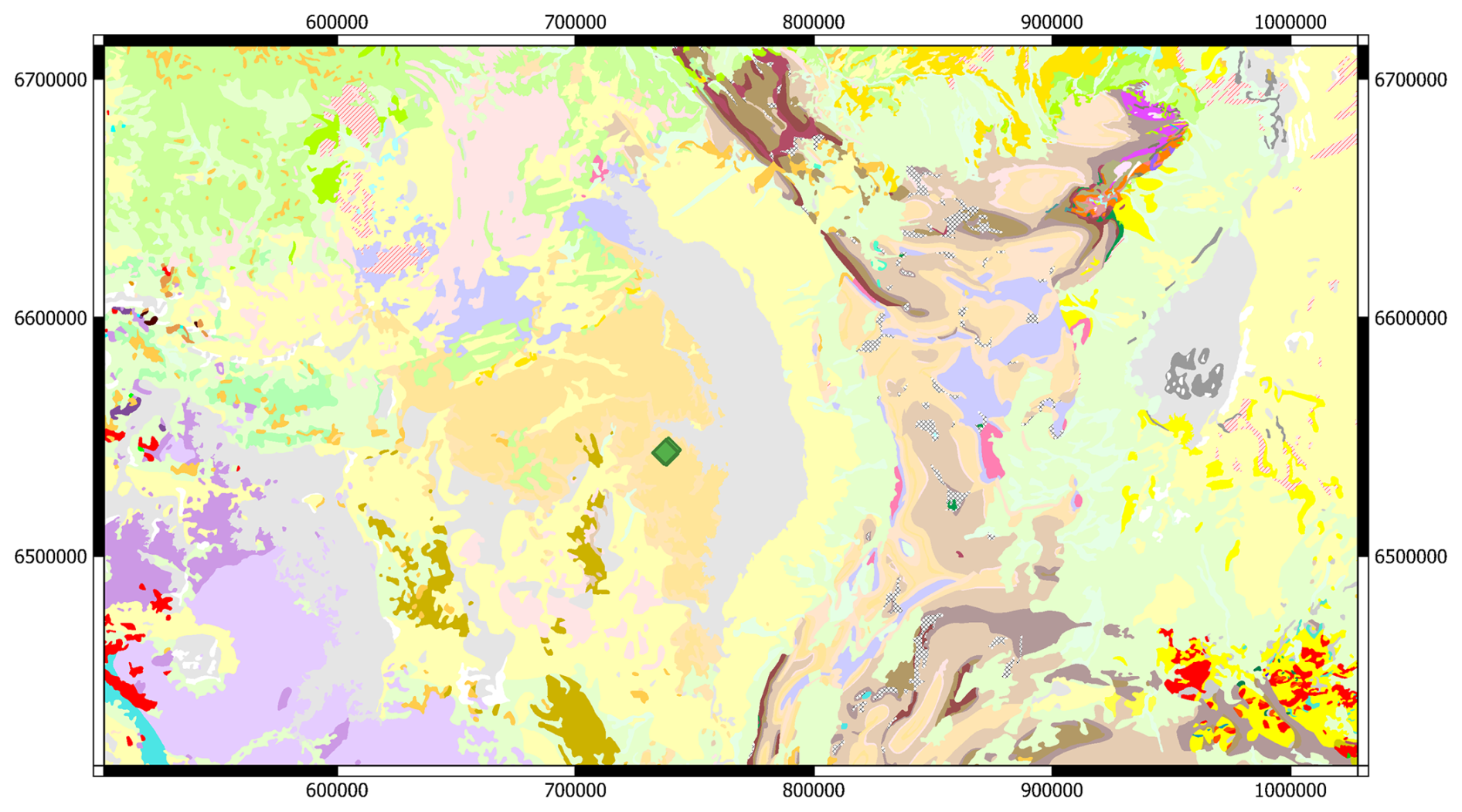
Figure 4 Location of South Australia test area (drillholes shown as green diamonds), together with an example stratigraphic log, map from 1:2 M Surface Geology Map of South Australia (The Department for Energy and Mining, the Government of South Australia, 2025, Geoscientific Data, Sourced on 22 July 2018).

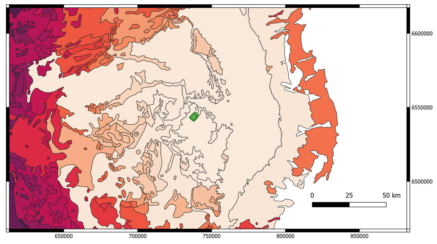
Figure 5 Distance of stratigraphic units from drillholes (darker colours signifies larger distance). Green diamonds show the location of the drillholes. Polygon source: The Department for Energy and Mining, the Government of South Australia (2025) Geoscientific Data, Sourced on 22 July 2018. Distance calculation as described in this paper.

To facilitate correlation analysis, we generalize the scoring function from Sect. 2.2 to evaluate any solution s_i against any local connectivity graph. Define the generalized scoring function as:

$$\begin{array}{}\text{(12)}& \mathrm{score}\left(s_i,G_h\right)={\displaystyle \frac{{\sum }_j{w}_h\left(u_j,u_{j+\mathrm{1}}\right)}{N_i}}\end{array}$$

where the sum is over all consecutive unit pairs ($u_j,u_{j+\mathrm{1}}$) in solution s_i, G_h represents any local connectivity graph derived from drillhole solutions, $w_h(u_j,u_{j+\mathrm{1}})$ denotes the edge weight from graph G_h for that unit pair, and N_i is the number of unit contacts in solution s_i. Note that G_h refers to local connectivity graphs from drillhole solutions, not the global connectivity graph Γ from map data (Sect. 2.2). If an edge $(u_j,u_{j+\mathrm{1}})$ from solution s_i does not exist in G_h, its weight is taken as zero. This generalized function allows us to assess how consistent a solution from one drillhole is with the geological relationships observed in other drillholes.

• Correlation Algorithm

  Consider a set of H drillholes $\mathit{\{}{h}_{\mathrm{1}},h_{\mathrm{2}},\mathrm{\dots },h\mathit{\_}H\mathit{\}}$ with their respective local connectivity graphs $\mathit{\{}{G}_{\mathrm{1}},G_{\mathrm{2}},\mathrm{\dots },G\mathit{\_}H\mathit{\}}$. For each solution s_i from any drillhole, we compute a correlated score that represents the average consistency across all drillholes:

  $$\begin{array}{}\text{(13)}& {\mathrm{score}}_{\mathrm{corr}}\left(s_i\right)={\displaystyle \frac{\mathrm{1}}{H}}{\sum }_{k=\mathrm{1}}^H{\mathit{\alpha }}_k\mathrm{score}\left(s_i,G_k\right)\end{array}$$

  where α_k are weighting factors that can be based on geological distance (distance between collar and closest node of map polygon), drillhole quality, or other criteria. This equation computes an average score across all drillholes. The division by H ensures the correlated score remains on a comparable scale regardless of the number of drillholes. In this work, we use α_k=1 for all drillholes, giving equal weight to each drillhole. This summation approach is robust to outliers; if one drillhole yields a zero score, it does not eliminate the entire correlation. Alternative weighting schemes such as inverse distance ${\mathit{\alpha }}_k=\mathrm{1}/d(h_{\mathrm{1}},h_k)$ could be employed to reduce the influence of more distant drillholes.

  The correlated scores are then normalized to obtain a revised probability distribution:

  $$\begin{array}{}\text{(14)}& P_{\mathrm{corr}}\left(s_i\right)={\displaystyle \frac{{\mathrm{score}}_{\mathrm{corr}}\left(s_i\right)}{{\sum }_m{\mathrm{score}}_{\mathrm{corr}}\left(s_m\right)}}\end{array}$$

  The correlated probability P_corr(s_i) provides a revised ranking of solutions that accounts for both local evidence and regional consistency. Solutions with unit contacts that appear frequently across multiple drillholes receive higher correlated scores, while solutions unique to a single drillhole receive lower scores. This correlation effectively reduces uncertainty by leveraging spatial geological consistency.

• Summation vs. Multiplication. While the equation for score_corr uses weighted summation, an alternative multiplicative approach could also be formulated. However, multiplicative forms are more sensitive to outliers: if any single drillhole yields a zero score, the entire correlated score becomes zero. Therefore, the summation approach is generally preferred for its robustness.

• Computational Efficiency. The algorithm achieves O(H²×S_avg) complexity when correlating solutions across all H drillholes, where S_avg represents the average number of solutions per drillhole. This efficiency is achieved by comparing solutions against pre-computed connectivity graphs G_h rather than performing pairwise solution comparisons. The alternative of solution-to-solution comparison would scale as $O(H^{\mathrm{2}}\times S_{\mathrm{avg}}^{\mathrm{2}})$ making it computationally prohibitive.

  By integrating and correlating drillhole data through this topological approach, we ensure that the stratigraphic framework accurately reflects the natural spatial variations and interconnections present in the subsurface. The correlation process quantitatively reduces uncertainty by identifying and favoring solutions that are geologically consistent across the broader area. This uncertainty reduction is achieved by concentrating probability mass on solutions supported by multiple drillholes while downweighting locally anomalous interpretations. The resulting correlated probabilities P_corr(s_i) provide more reliable stratigraphic interpretations than single-drillhole probabilities P(s_i), enabling more informed decisions in geological exploration and 3D geological modeling.

Figure 6 Topological relationships between units in and around the test area.

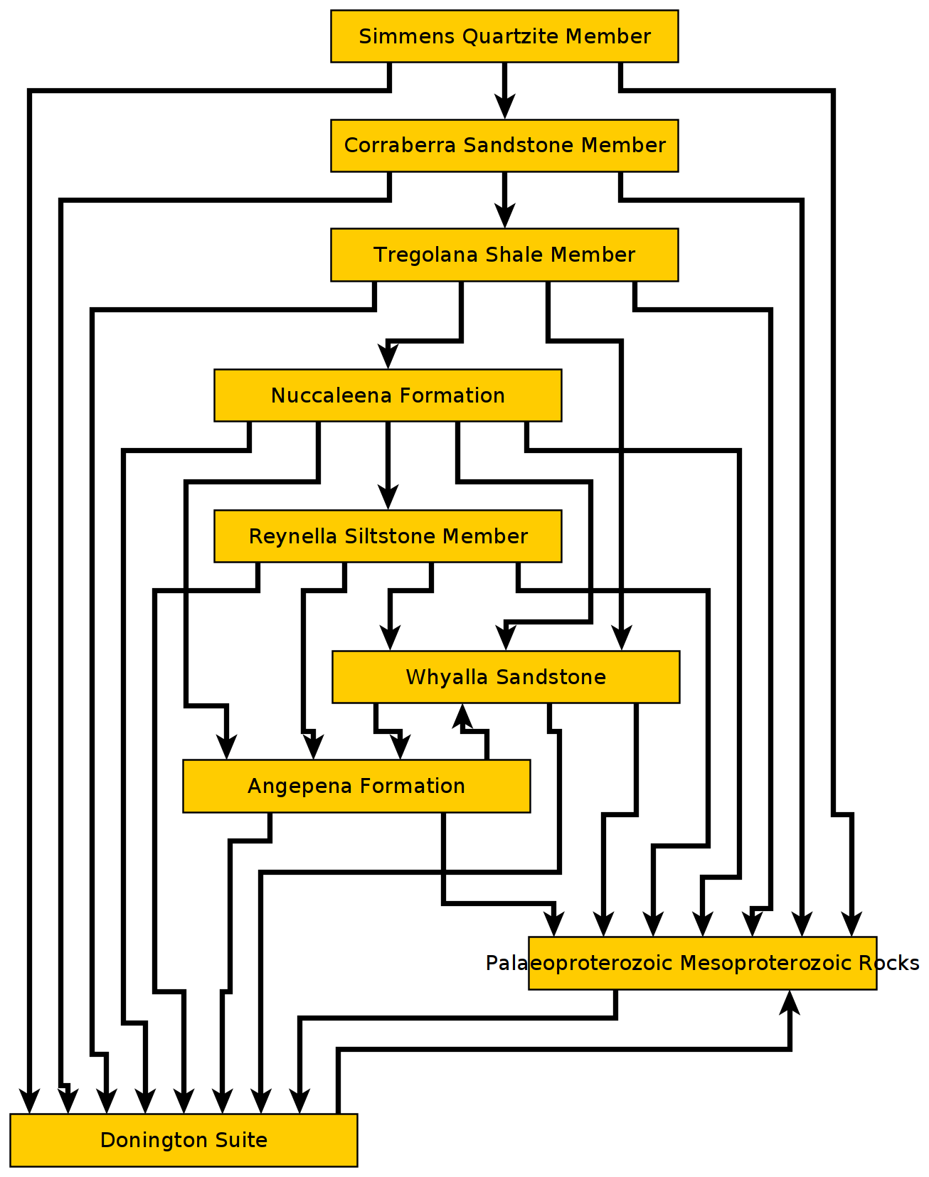
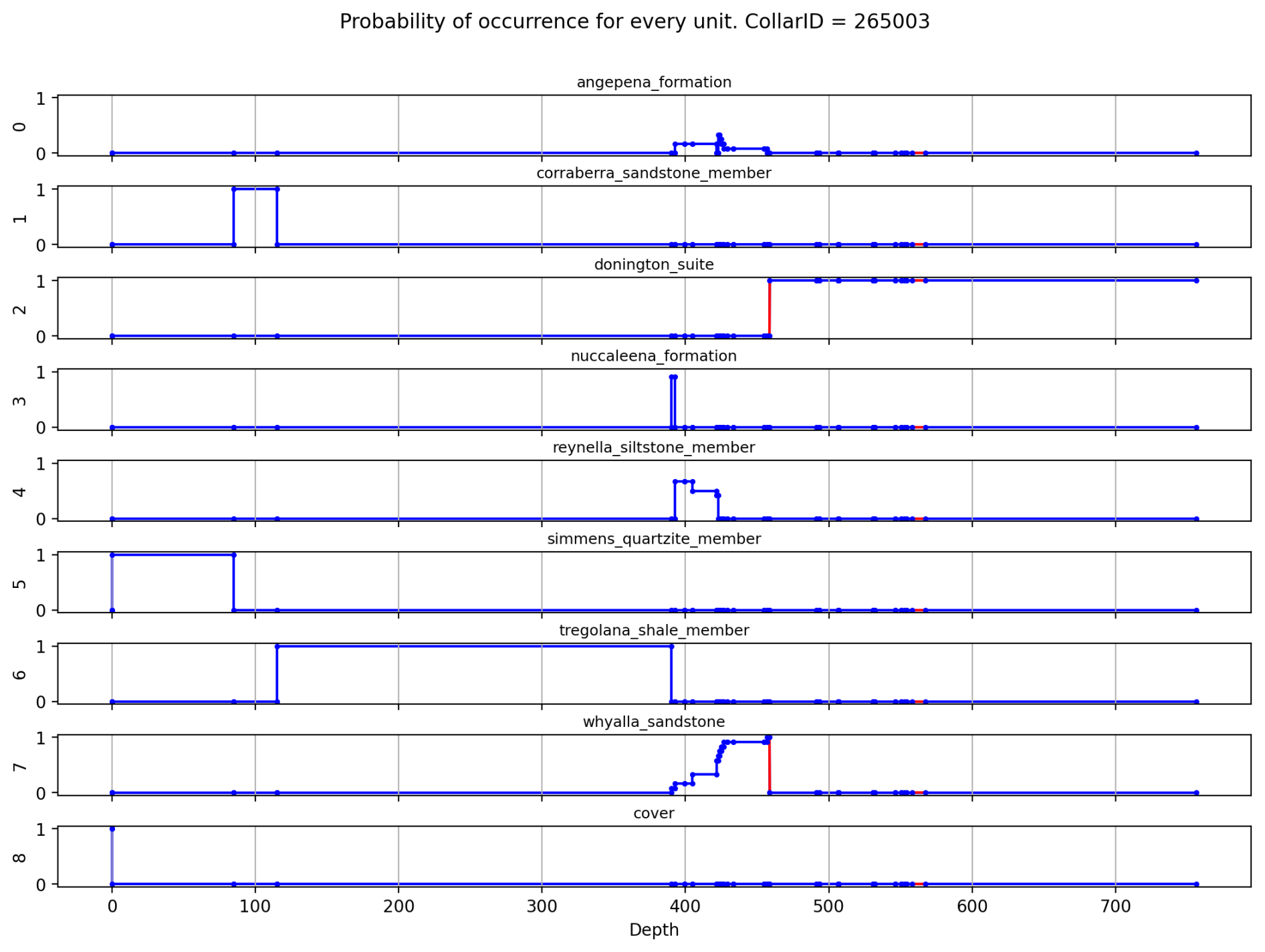
Figure 7 Estimated probability of each stratigraphic unit occurring at a given depth for a single drillhole.

2.6 Code design

A Python package called litho2strat has been developed for stratigraphy recovery. It can be easily installed using the command “pip install”, and it has minimal external library dependencies: numpy, matplotlib, and NetworkX. The NetworkX library is utilized to create a directed graph data structure that represents the topological relationships of relative unit ages (Hagberg et al., 2008). It also supports exporting graphs to GML format (Himsolt, 1997) for advanced graph visualization with tools like yEd (https://www.yworks.com/products/yed, last access: 27 January 2026). Interaction with the code is facilitated through a Parfile, a text file that contains all necessary parameters and paths to the input data files. The parameters in the Parfile are organized into several categories based on their functionality, including input file paths, solver settings, and data preprocessing options. An example of such a Parfile is provided in Appendix B.

The code architecture efficiently organizes distinct modules, including data reader, the user interface (represented by the Parfile), the algorithms (such as the solver), and the visualization components (e.g., output figures and graphs), as shown in Fig. 3. This design enhances code readability, making it easier for developers to understand and navigate the codebase. Additionally, it facilitates further extensions by allowing new features to be integrated seamlessly. This structure also supports effective testing, enabling modifications to be verified systematically and reducing the risk of introducing errors.

3 Example Use

For this example, we used a set of 52 drillholes from South Australia originally drilled by Teck Cominco Pty. Ltd. (Fig. 4). This area was chosen as there were a number of holes equally spaced with a relatively homogenous spatial distribution and the holes provided both lithological logs and existing interpretations of the down-hole stratigraphy.

3.1 Data Cleaning

Examples of terms in the ignore list for this case study include the following, where each term is excluded from drillhole lithology log processing:

1. Breccia (Undiff. Origin)

2. Ironstone (Metasomatic)

3. No Information

4. Solution-Collapse Breccia

5. Vein (Undifferentiated)

Examples of the thesaurus of synonyms for this case study area include the following groups, where each group contains lithology names that are treated as equivalent:

1. dolomite, dolomite rock, carbonate rock, limestone

2. conglomerate, diamictite

3. grit, sandstone, quartzite, siltstone

4. gabbro, gabbronorite

3.2 Map Analytics

Figure 5 shows stratigraphic units coloured as a function of the distance to one of the drillholes. A large search area was used for this example as the stratigraphy is fairly flat lying so there is no guarantee that a unit will reach the surface in the local neighbourhood.

In the initial analysis we constructed the global connectivity graph Γ (Sect. 2.2), representing topological relationships between stratigraphic units. The initial graph was constructed automatically from the geological map (extending out 100 km from the test area) using the map2model software, then manually extended with additional topological relationships from the ASUD database and published reports. The graph was processed using the NetworkX Python library, exported to GML format, and visualized using yEd software (Fig. 6). The global connectivity graph consists primarily of single-direction edges, with two bidirectional edges (Whyalla Sandstone–Angepena Formation and Paleoproterozoic-Mesoproterozoic Rocks–Donington Suite) to account for spatial variability in their stratigraphic relationships.

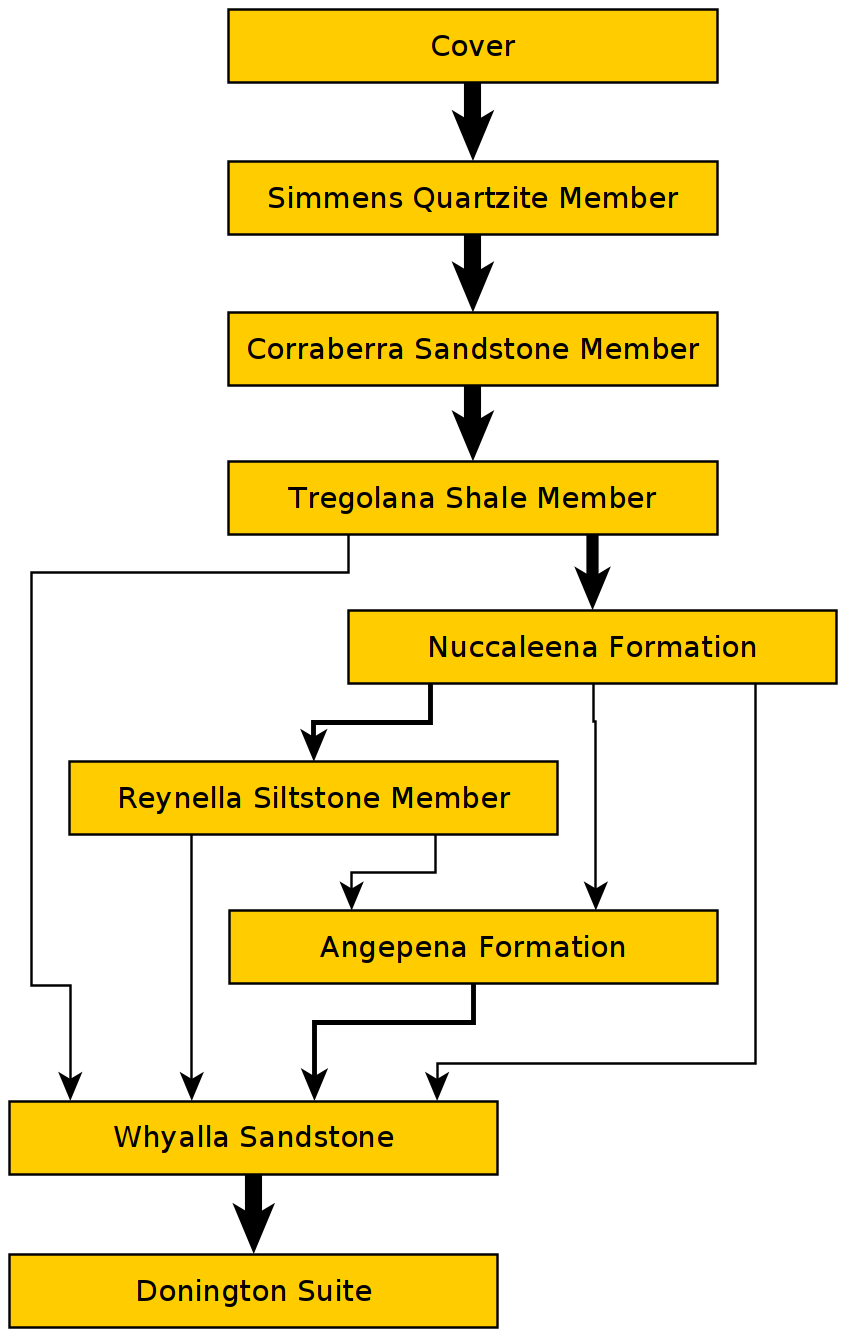
Figure 8 Calculated local topology using all solutions. Graph edges (relationships) between two stratigraphic units are displayed as the probability of that contact-relationship occurring.

3.3 Drillhole Analytics

The drillhole analysis calculated every possible stratigraphic ordering that was consistent with the observed lithological ordering down the drillhole and solution constraints (described in Sect. 2.3). By collating the results for all possible solution paths, we can produce estimates of the marginal probability that any depth interval will be a particular stratigraphic unit (Fig. 7). For depth interval i and stratigraphic unit u, the probability P_i(u) is computed as:

$$\begin{array}{}\text{(15)}& P_i\left(u\right)={\displaystyle \frac{\left|\mathit{\{}s\in S:s\left[i\right]=u\mathit{\}}\right|}{\left|S\right|}}\end{array}$$

where S is the set of all valid solutions and s[i] denotes the unit assigned to interval i in solution s.

In Fig. 8, we present the final (local) unit connectivity derived from the stratigraphic solutions generated. The width of the graph edges indicates the probability of unit contacts, with thicker edges signifying higher probabilities. This visual representation allows for a clear comparison of connectivity before (Fig. 6) and after the stratigraphic analysis.

The final solution score for a single ordering is calculated by summing of the probabilities of the contact edge weights. This allows us to sort the orderings by probability, ignoring stratigraphic thickness for now (Fig. 9).

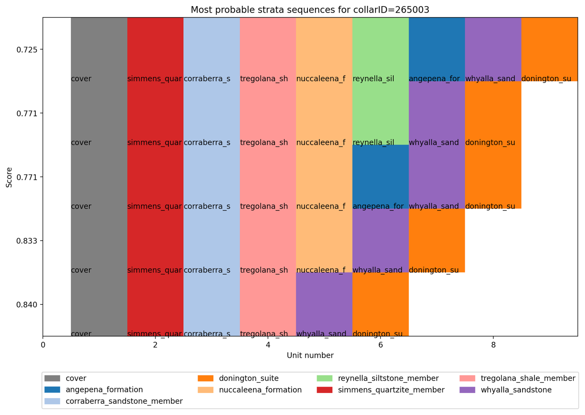
Figure 9 The 5 most probable stratigraphic orderings, with their solution probability on the x axis and order of depth on the y axis.

Finally, we can then include the depths to contacts between units in the drillhole based on the previous analyses (Fig. 10).

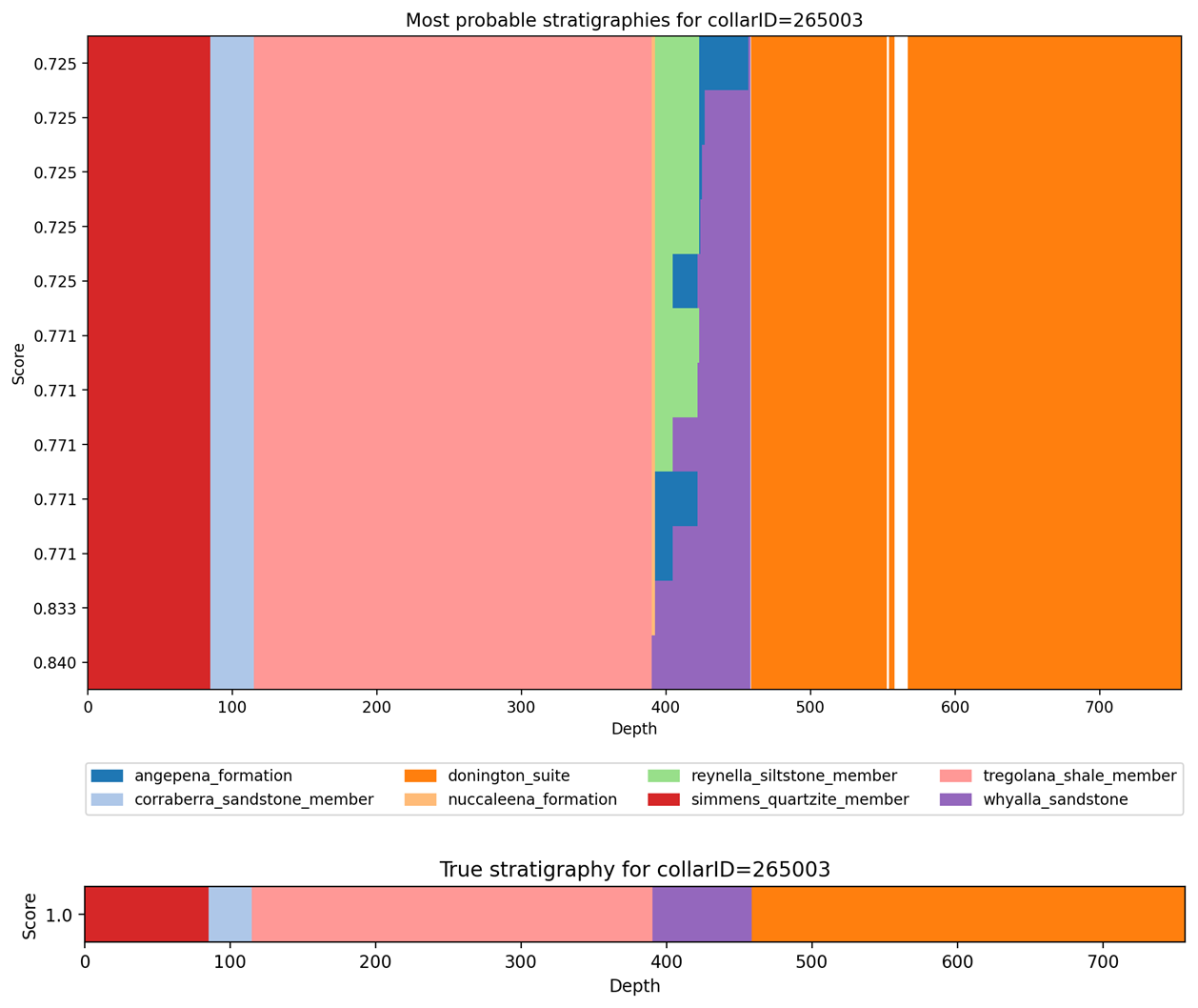
Figure 10 The 12 most probable stratigraphic orderings showing true depth of contact (above) compared to the stratigraphy as logged for the same hole.

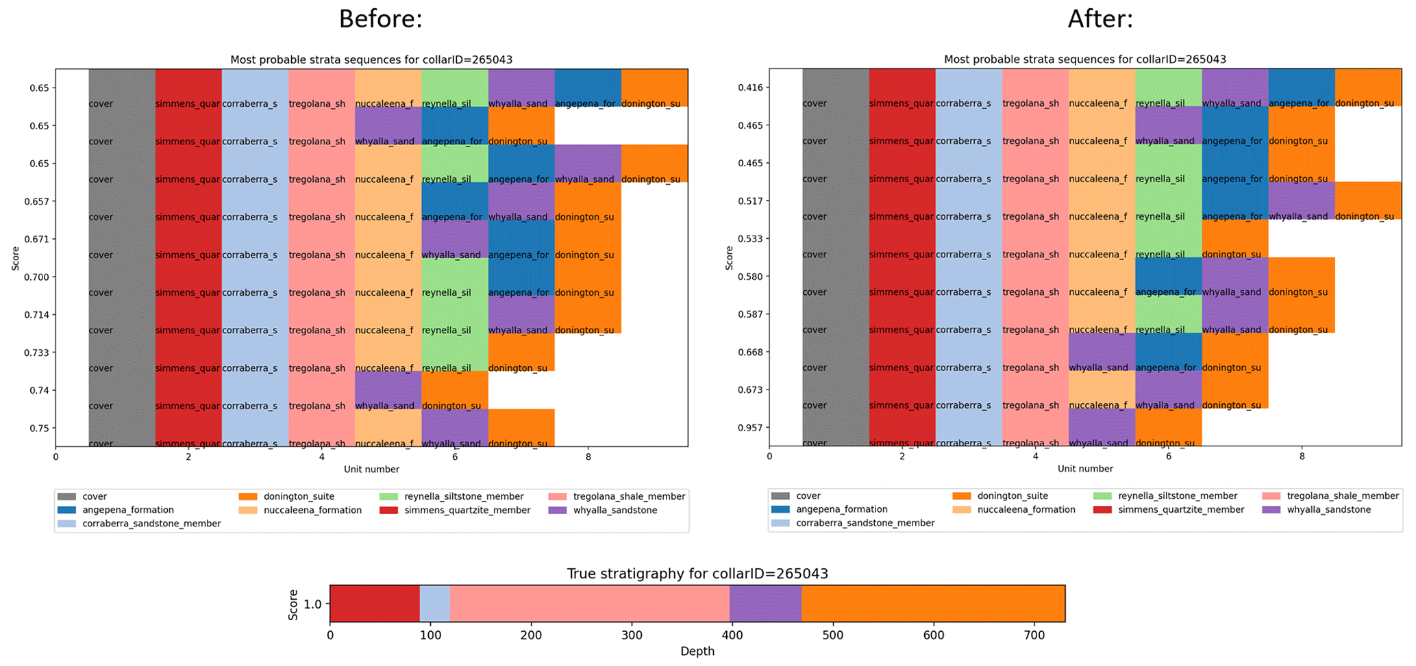
Figure 11 Comparison of ordering for one hole (left) vs ordering for that hole considering the outcomes of 45 other drillholes in the neighbourhood.

In the next stage of our analysis, we perform solution correlation across multiple drill holes to establish a plausible stratigraphic order and reduce uncertainty. Figure 11 illustrates the comparison of the most probable stratigraphies before and after correlation. Prior to correlation, the solution that aligns with the “true” stratigraphy (the correct solution) is ranked second, with a score of S=0.74, while the highest-ranked solution has a score of S=0.75. However, after applying the correlation, the correct solution rises to the top rank with a score of S=0.95, whereas the previously highest-ranked solution falls to second place with a score of S=0.67. This correlation analysis not only helped identify the correct solution but also significantly reduced its relative uncertainty, increasing the relative score between the top two solutions from 1 % to 42 %. The computational efficiency of the litho2strat algorithm was evaluated through performance testing on this dataset, with scalability analysis presented in Appendix A.

4 Discussion and Future Work

Whilst we were able to develop a workflow that successfully provided useful stratigraphic analyses for our test area, we recognise that for other areas the methodology was not always as successful. We have identified several aspects of the current stratigraphic descriptions that we think will significantly expand the useability of the workflow we present above.

1. Lithological Uncertainty. Vague lithological descriptions are a major limitation. In many areas, the lithological descriptions of stratigraphic units are quite vague, and successive stratigraphic units in a group might have very similar lithological descriptions..

   As an example, we look at the Hamersley Group, in Western Australia (Maldonado and Mercer, 2018). If we examine the GSWA explanatory notes for three successive formations (Mt McRae Shale, Mt Sylvia Formation and the Wittenoom Formation) in the GSWA explanatory notes their lithologies are described as:

   • –

     Mt McRae Shale – Mudstone, siltstone, chert, iron-formation, and dolomite. Thin bands of shard-bearing volcanic ash in upper parts.

   • –

     Mt Sylvia Formation – Mudstone, siltstone, chert, iron-formation, and dolomite.

   • –

     Wittenoom Formation – Thinly bedded dolomite and dolomitic shale, with minor black chert, shale, banded iron formation and sandstone.

   We can see that there is a significant overlap in lithologies, with an ordering of lithologies but without constraints on the percentage of each lithology in the three formations. This additional information, even as an estimate, would provide useful constraints on the likelihood that a specific lithology is associated with a given stratigraphic unit.

2. Min–Max thickness estimates. In some areas, there is useful information on the minimum, maximum and average stratigraphic thickness of units.

3. Stratigraphic ordering of lithologies. Additional information on commonly occurring orderings of lithologies within a given formation or member would also provide useful constraints.

   All three of these types of information are often included in the free-text portions of stratigraphic databases, such as the example shown for the West Angela Member in the GSWA Explanatory Notes in Fig. 12. In this example the free text provides more specific information on the thickness, the ordering of lithologies and the relative proportions of lithologies. With the advent of more sophisticated Machine Learning methodologies, the extraction of this ancillary data in a standardised form from reports and the stratigraphic databases themselves will open up new possibilities for constraining stratigraphy. Similarly, the codes developed in dh2loop for harmonising lithological terminologies will expand greatly in coming years.

4. Inclusion of discontinuity information in the litho2strat workflow (most often logged faults) could help to define where breaks in stratigraphy are most likely to occur

5. Inclusion of secondary descriptive information (for example grain size) could help to refine our younging estimators in areas of uncertain facing.

6. There is no doubt that the advent of Large Language Models will have a profound effect on our ability to extract and categorize information from unstructured data sources, and algorithms based on these approaches will probably replace the data extraction and data harmonisation modules in future versions of this workflow.

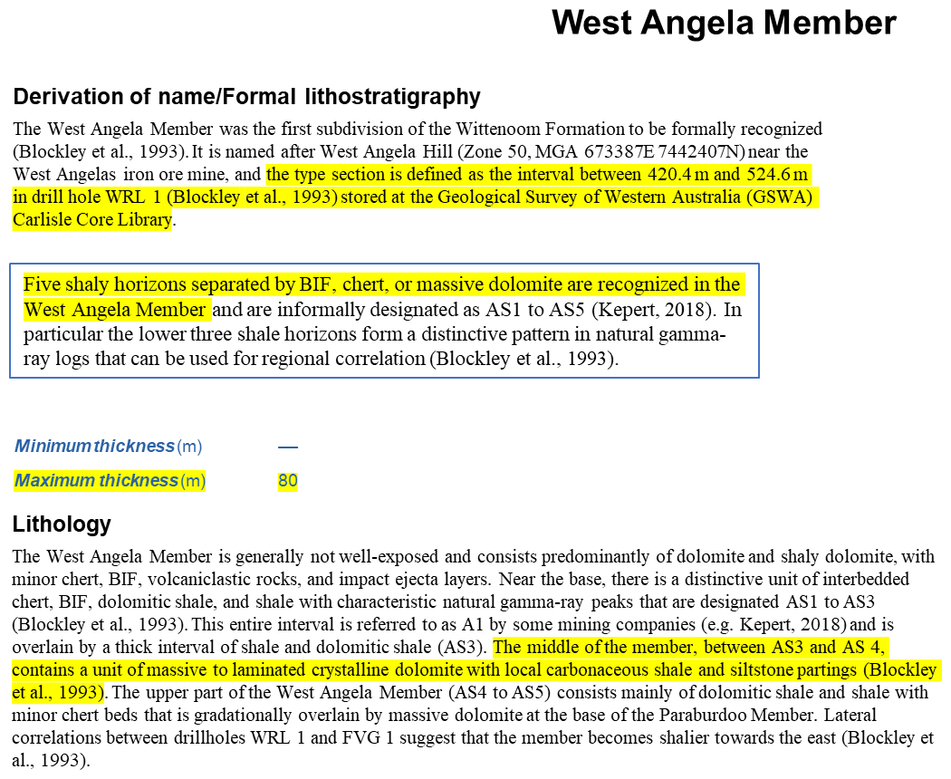
Figure 12 Free-text descriptions of the West Angela Member in the GSWA Explanatory Notes. (Geological Survey of Western Australia (GSWA), 2024. Explanatory Notes System accessed via GeoVIEW.WA, https://geoview.dmp.wa.gov.au/geoview/, last access: 1 June 2024.)

5 Conclusions

We developed codes and methodologies for stratigraphy recovery from drillhole databases, utilizing the branch and prune algorithm as a foundational framework. To ensure the generation of geologically plausible solutions, we implemented various types of constraints that account for the complexities of subsurface geology. To further reduce uncertainty in the obtained solutions, we introduced a correlation algorithm that leverages information from multiple drillholes simultaneously. This innovative approach allows for a more robust analysis by integrating data across different locations, enhancing the reliability of the stratigraphic interpretations.

Our proposed method was applied to a dataset comprising 52 drillholes from South Australia. The results demonstrated that the algorithm successfully predicts the correct stratigraphic solution while providing associated uncertainty metrics, effectively validating its performance against measured stratigraphy data.

Additionally, we identified several key aspects of the current stratigraphic descriptions that could significantly enhance the usability of the workflow we have presented. These enhancements aim to improve the accessibility and applicability of our methodology, paving the way for more effective geological assessments and decision-making processes in the field.

Appendix A: Performance and Scalability Analysis

To complement the theoretical complexity analysis presented in Sect. 2.4, we conducted empirical tests to evaluate the performance and scalability of the litho2strat algorithm. We tested how the average number of solutions maintained during recursive exploration (N) scales with the number of lithology changes in drillhole logs, comparing two scenarios: (1) using the global topology graph Γ as a constraint, and (2) without topology constraints.

Figure A1 shows the relationship between the number of lithology changes and the average number of solutions maintained during recursive exploration when the topology graph constraint is applied. The results demonstrate near-linear scaling, confirming that the topology graph effectively prunes the solution space while preserving geological validity.

Figure A2 presents the same relationship for the unconstrained case, where the algorithm considers all theoretically possible stratigraphic interpretations. Here, the average number of solutions maintained during recursive exploration exhibits near-exponential growth with increasing lithology changes, illustrating the combinatorial explosion that occurs without geological constraints.

The computational performance measurements further highlight the practical importance of these constraints. Using a single CPU core (Intel i7-1185G7 @ 3.00 GHz) to process all 52 drillholes from Sect. 3 and perform the correlation of solutions, the constrained approach required approximately 1 s total processing time, while the unconstrained case required approximately 50 s for the same dataset. This 50-fold improvement in computational efficiency, combined with the near-linear versus near-exponential scaling behavior of solutions maintained during recursive exploration, demonstrates that incorporating geological knowledge through the topology graph is essential for both computational tractability and practical applicability of the litho2strat algorithm to real-world geological datasets.

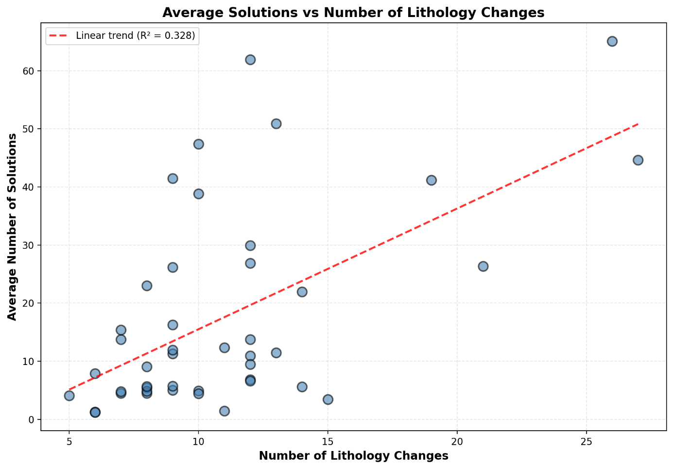
Figure A1 Average number of solutions maintained during recursive exploration versus number of lithology changes with topology graph constraint.

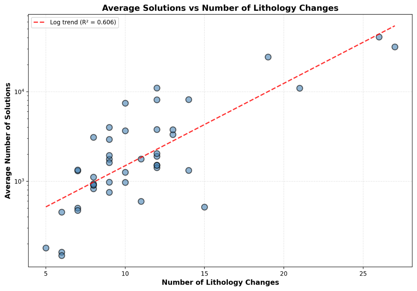
Figure A2 Average number of solutions maintained during recursive exploration versus number of lithology changes without topology constraints.

Appendix B: Control file for litho2strat code

Example usage: python3 litho2strat.py -p ./parfiles/Parfile_SA.txt

Example parfile:

[FilePaths]
topology_filename = data/SA_test_data/newpairs_20_06_2023.gml
ignore_list_filename = data/SA_test_data/ignore_list.txt
alternative_rock_names_filename = data/SA_test_data/alternative_rock_names.txt
unit_colors_filename = data/SA_test_data/unit_colors.csv

drillsample_filename = data/SA_test_data/litho_tables/litho_$collarID$.csv
stratasample_filename = data/SA_test_data/strat_tables/strat_$collarID$.csv
dist_table_filename = data/SA_test_data/dh_asud_strat2.csv

[DataHeaders]
drillsample_header = DEPTH_FROM_M, DEPTH_TO_M, MAJOR_LITHOLOGY,
stratasample_header = DEPTH_FROM_M, DEPTH_TO_M, STRAT_UNIT_NAME,
strata_data_header = strat, summary, distance, description

[SolverParameters]
add_topology_constraints = True
max_num_strata_jumps = 0
max_num_returns_per_unit = 0
max_num_unit_contacts_inside_litho = 0
single_top_unit = True

[DataPreprocessing]
number_nearest_units = 10
min_drillhole_litho_score = 80
group_drillhole_lithos = False
cover_ratio_threshold = 0.65

[CollarIDs]
collarIDs = 205821,205822,264999,265000,265001