the Creative Commons Attribution 4.0 License.
the Creative Commons Attribution 4.0 License.
 | 10 Dec 2025
LISFLOOD-FP 8.2: GPU-accelerated multiwavelet discontinuous Galerkin solver with dynamic resolution adaptivity for rapid, multiscale flood simulation
Alovya Ahmed Chowdhury
Georges Kesserwani
The second-order discontinuous Galerkin (DG2) solver of the two-dimensional shallow water equations in the raster-based LISFLOOD-FP 8.0 hydrodynamic modelling framework is mostly suited for predicting small-scale transients that emerge in rapid, multiscale floods caused by impact events like tsunamis. However, this DG2 solver can only be used for simulations on a uniform grid where it may yield inefficient runtimes even when using its graphics processing unit (GPU) parallelised version (GPU-DG2). To boost efficiency, the new LISFLOOD-FP 8.2 version integrates GPU parallelised dynamic (in time) grid resolution adaptivity of multiwavelets (MW) with the DG2 solver (GPU-MWDG2). The GPU-MWDG2 solver performs dyadic grid refinement, starting from a single grid cell, with a maximum refinement level, L, based on the resolution of the Digital Elevation Model (DEM). Furthermore, the dynamic GPU-MWDG2 adaptivity is driven by one error threshold, ε, against normalised details of all prognostic variables. Its accuracy and efficiency, as well as the practical validity of recommended ε choices between 10−4 and 10−3, are assessed for four laboratory/field-scale benchmarks of tsunami-induced flooding with different impact event complexities (i.e. single- vs. multi-peaked) and L values. Rigorous accuracy and efficiency metrics consistently show that GPU-MWDG2 simulations with ε = 10−3 preserve the predictions of the GPU-DG2 simulation on the uniform DEM grid, whereas ε = 10−4 may slightly improve velocity-related predictions. Efficiency-wise, GPU-MWDG2 yields considerable speedups from L ≥ 10 – due to its scalability on the GPU with increasing L – which can be around 2.0-to-4.5-fold. Generally, the bigger the L ≥ 10, the lower the event complexity over the simulated duration, and the closer the ε to 10−3, the larger the GPU-MWDG2 speedups over GPU-DG2. The LISFLOOD-FP 8.2 code is open source, under the GPL v3.0 licence, as well as the simulated benchmarks' set-up files and datasets, with a video tutorial and further documentation on https://www.seamlesswave.com/Adaptive (last access: 6 July 2025).
- Article
(16494 KB) - Full-text XML
- BibTeX
- EndNote


LISFLOOD-FP is a raster-based hydrodynamic modelling framework that has been used to support various geoscientific modelling applications (Hajihassanpour et al., 2023; Hunter et al., 2005; Nandi and Reddy, 2022; Zeng et al., 2022; Ziliani et al., 2020). LISFLOOD-FP has a suite of numerical solvers of the two-dimensional shallow water equations, for which the prognostic variables are the time-variant water depth h (m) and unit-width discharges hu and hv (m2 s−1) and time-invariant topography z (m), all represented as raster-formatted data on a uniform grid at a Digital Elevation Model (DEM) resolution. It includes a diffusive wave solver (Hunter et al., 2005), a local inertial solver (Bates et al., 2010), a first-order finite volume solver, and a second-order discontinuous Galerkin (DG2) solver (Shaw et al., 2021), all already supported with robustness treatments (i.e. for topographic and friction discretisation with wetting and drying), ensuring numerical mass conservation to machine precision. The DG2 solver is the most complex numerically, requiring three times more modelled data (degrees of freedom) per prognostic variable and at least twelve times more computations per cell compared to any of the other solvers in LISFLOOD-FP. This complexity arises from its locally conservative formulation that pays off with more inherent mimetic properties (Ayog et al., 2021; Kesserwani et al., 2018), i.e. numerical momentum conservation and reduced (spurious) error dissipation, leading to more accurate velocity fields and long-duration flood simulations (Ayog et al., 2021; Kesserwani and Sharifian, 2023; Sun et al., 2023). Thus, even when parallelised on a graphics processing unit (GPU), the GPU parallelised DG2 solver (GPU-DG2) may still have prohibitively long runtimes, e.g. when applied to run simulations at DEM resolutions close to 1 m and/or with DEM grid sizes beyond 1 km (Kesserwani and Sharifian, 2023; Shaw et al., 2021).
DG2 simulations were shown to accurately reproduce slow to gradual fluvial/pluvial flooding flows at unusually coarse DEM resolutions (Ayog et al., 2021; Kesserwani, 2013; Kesserwani and Wang, 2014), but they primarily excel at capturing the small-scale rapid flow transients that occur over a wide range of spatial and temporal scales (Kesserwani and Sharifian, 2023; Sharifian et al., 2018; Sun et al., 2023). Such transients are typical of flooding flows driven by impact event(s) like tsunami(s) and including zones of flow recirculation past (un)submerged island(s). Hence, DG2 simulations are likely suited for obtaining accurate modelling of rapid, multiscale flooding, such as for tsunami-induced inundations. Within this scope, dynamic (in time) mesh adaptivity has often been deployed with finite volume based tsunami simulators to reduce simulation runtimes (Lee, 2016; Popinet, 2012). This paper reports the integration of dynamic grid resolution adaptivity into the GPU-DG2 solver in a new LISFLOOD-FP 8.2 release to reduce the runtimes of rapid, multiscale flow simulations, which are here exemplified by tsunami-induced flooding events.
Unlike static grid resolution adaptivity (Kesserwani and Liang, 2015) – integrated into LISFLOOD-FP 8.1 with the reduced-complexity finite volume solver (Sharifian et al., 2023) – this LISFLOOD-FP 8.2 version performs dynamic grid resolution adaptivity with the DG2 solver every global simulation timestep Δt to achieve as much local grid resolution coarsening as possible. Namely, grid coarsening is applied to the grid cells covering either regions of smooth flow or DEM features, thereby reducing the number of computational cells as much as allowed by the complexity of the DEM and flow solution. The LISFLOOD-FP 8.2 version is unique in providing a single, mathematically sound hydrodynamic modelling framework that implements dynamic grid resolution adaptivity entirely on the GPU for achieving raster-grid DG2 simulations that can preserve a similar level of predictive accuracy and robustness as alternative GPU-DG2 simulations on a uniform grid. The framework is formulated in Kesserwani and Sharifian (2020), having been informed by Caviedes-Voullième and Kesserwani (2015), Gerhard et al. (2015), Kesserwani et al. (2015) and Caviedes-Voullième et al. (2020), so as to preserve all the mimetic properties inherent in the reference DG2 hydrodynamic solver (Kesserwani et al., 2018; Kesserwani and Sharifian, 2023). Here, it has been computationally optimised and integrated into LISFLOOD-FP 8.2, in which dynamic grid resolution adaptivity of multiwavelets (MW) is combined with the DG2 solver formulation. This combination is hereafter referred to as dynamic GPU-MWDG2 adaptivity or the GPU-MWDG2 solver.
Existing hydrodynamic modelling frameworks that have integrated dynamic grid resolution adaptivity with GPU parallelisation were mostly based on finite volume solvers (Berger et al., 2011; Ferreira and Bader, 2017; Kevlahan and Lemarié, 2022; de la Asunción and Castro, 2017; LeVeque et al., 2011; Liang et al., 2015; Park et al., 2019; Popinet, 2011, 2012; Popinet and Rickard, 2007). Comparatively, fewer are based on DG solvers that are mostly developed for tsunami inundation simulation on triangular or curvilinear meshes, with sparse focusses: either on achieving parallelisation on central processing units (CPU) with extrinsic forms of dynamic resolution adaptivity, or on parallelising non-adaptive DG solvers on the GPU; while, in any of the focusses, addressing robustness treatments (Blaise et al., 2013; Blaise and St-Cyr, 2012; Bonev et al., 2018; Castro et al., 2016; Hajihassanpour et al., 2019; Rannabauer et al., 2018). To mention just a few, Blaise and St-Cyr (2012) and Blaise et al. (2013) integrated CPU parallelisation into dynamic adaptivity for curvilinear meshes, calling for better forms of adaptivity with improved robustness treatments to achieve reliable DG based tsunami inundation simulations. Rannabauer et al. (2018) addressed wetting and drying treatments with a DG based solver of tsunami inundation that integrated CPU parallelised dynamic adaptivity on triangular meshes; further, the authors identified the benefit of their DG based solver compared to the finite volume solver counterpart. To track tsunami propagation on the sphere, Bonev et al. (2018) and Hajihassanpour et al. (2019) devised DG based solvers with dynamic adaptivity for curvilinear meshes, highlighting the need to further exploit GPU parallelisation to achieve realistic runtimes. For tsunami inundation simulations, Castro et al. (2016) found that non-adaptive DG simulations on triangular meshes to be 23-fold faster when parallelised on the GPU compared to parallelised simulations on the CPU with 24 threads.
Yet, to the best of the authors' knowledge, there is no existing DG based hydrodynamic modelling framework that combines raster grid-based dynamic resolution adaptivity with GPU parallelisation within a mathematically sound framework, i.e. one that preserves the mimetic properties of the reference robust DG2 solver on the uniform grid (Kesserwani et al., 2019; Kesserwani and Sharifian, 2020, 2023) like the dynamic GPU-MWDG2 adaptivity integrated into LISFLOOD-FP 8.2. To elaborate, the MWDG2 solver automates local grid resolution coarsening on an adaptive grid using the multiresolution analysis (MRA) of MW applied to scaled DG2 modelled data (for all the prognostic variables) that exist in a hierarchy of grids. This hierarchy consists of dyadically coarser grids relative to the finest grid in the hierarchy (Kesserwani et al., 2019; Kesserwani and Sharifian, 2020; Sharifian et al., 2019), whereby the finest resolution grid is associated with a maximum refinement level, L, and consists of 2L × 2L cells – with L selected to match the resolution of a raster-formatted DEM file. Meanwhile, the coarsest resolution grid consists of 20 × 20 = 1, i.e. a single cell. On the hierarchy of grids, the scaled DG2 modelled data for each prognostic variable are compressed into higher-resolution MW coefficients, or details, which are added to the coarsest resolution data. The details of all the prognostic variables are normalised and packed in a dataset of normalised details, which are then compared to an error threshold 0 < ε < 1 for retaining the significant details. The retained significant details are added to the coarsest resolution DG2 modelled data, leading to a multiscale representation of DG2 modelled data on a non-uniform grid. As the scaling, analysis, and reconstruction of DG2 modelled data are inherent to the MRA procedure, the mimetic properties of the reference GPU-DG2 solver on the finest resolution grid (2L × 2L) can readily be preserved for ε ≤ 10−3, based on studies considering a range for ε between 10−6 to 10−1 (Kesserwani et al., 2019; Kesserwani and Sharifian, 2020). Another benefit of the MRA procedure is the sole reliance on ε to sensibly control the amount of local grid resolution coarsening for all prognostic variables. Furthermore, it was also shown that, for the same ε, dynamic MWDG2 adaptivity avoids unnecessary refinement compared to its first-order counterpart, and using ε ≥ 10−4 leads to simulations that are faster than first-order finite volume solvers on the finest resolution grid (Kesserwani and Sharifian, 2020).
The dynamic MWDG2 adaptivity integrated in LISFLOOD-FP 8.2 optimises the approach proposed in Kesserwani and Sharifian (2020), which was initially designed for realistic, two-dimensional hydrodynamic modelling on a single core CPU and was based on the reference DG2 hydrodynamic solver in Kesserwani et al. (2018). Chowdhury et al. (2023) devised a computationally efficient GPU implementation of wavelet adaptivity integrated with a first-order finite volume (FV1) solver counterpart. They reported that the speedup of their GPU implementation over the uniform FV1 solver run on the finest 2L × 2L resolution grid scaled up with increasing L, becoming considerable for L≥9. In fact, for L≥9, there would be enough memory and compute workload to bound the GPU, which the adaptive solver can reduce unlike the uniform solver. Kesserwani and Sharifian (2023) extended the GPU implementation of Chowdhury et al. (2023) to produce the GPU-MWDG2 solver. They analysed its efficiency for ε = 10−3 in simulating realistic flooding flow scenarios for adaptive grids involving L ≥ 10. Their findings revealed that the GPU-MWDG2 solver is 3-fold faster than the GPU-DG2 solver on the finest resolution grid for a rapid flood scenario driven by an impact event, where dynamic GPU-MWDG2 adaptivity did not use more than 85 % of the number of cells of GPU-DG2. Hence, a dedicated study is needed to further analyse the usability and practical merit of GPU-MWDG2 simulations over GPU-DG2 simulations for rapid multiscale flooding scenarios.
Next, in Sect. 2, the GPU-MWDG2 solver in LISFLOOD-FP 8.2 is described with a focus on its use for running GPU-MWDG2 simulations from raster-formatted DEM and initial flow setup files (Sect. 2.1), its associated upper memory limits and scalability (Sect. 2.2), and analysis of efficiency using newly proposed metrics (Sect. 2.3). In Sect. 3, the efficiency and accuracy of the GPU-MWDG2 solver are assessed against the GPU-DG2 solver, with choices of ε = 10−3 and 10−4, for four tsunami-induced flooding benchmarks at both laboratory- and field-scale. Section 4 draws conclusions and recommendations as to when the GPU-MWDG2 solver can best be used over the GPU-DG2 solver. The LISFLOOD-FP 8.2 code is open-source, under the GPL v3.0 licence (LISFLOOD-FP developers, 2024), as well as the simulated benchmarks' set-up files and datasets (Chowdhury, 2024), a video tutorial (Chowdhury, 2025) and documentation on https://www.seamlesswave.com/Adaptive.
LISFLOOD-FP 8.2 includes the new capability of running simulations over a non-uniform grid using dynamic GPU-MWDG2 adaptivity. The GPU-MWDG2 solver can be used as an alternative to the uniform-grid GPU-DG2 solver (Shaw et al., 2021) to potentially reduce simulation runtimes. Unlike with LISFLOOD-FP 8.1, where the MRA procedure of MW is only applied once at the beginning of the simulation to generate a static non-uniform grid whose grid resolution is locally coarsened as much as permitted by features of the time-invariant DEM features (Sharifian et al., 2023), the GPU-MWDG2 solver deploys the MRA procedure every global simulation timestep, denoted by Δt, to also automate grid resolution coarsening based on the features of the time-varying flow solutions.
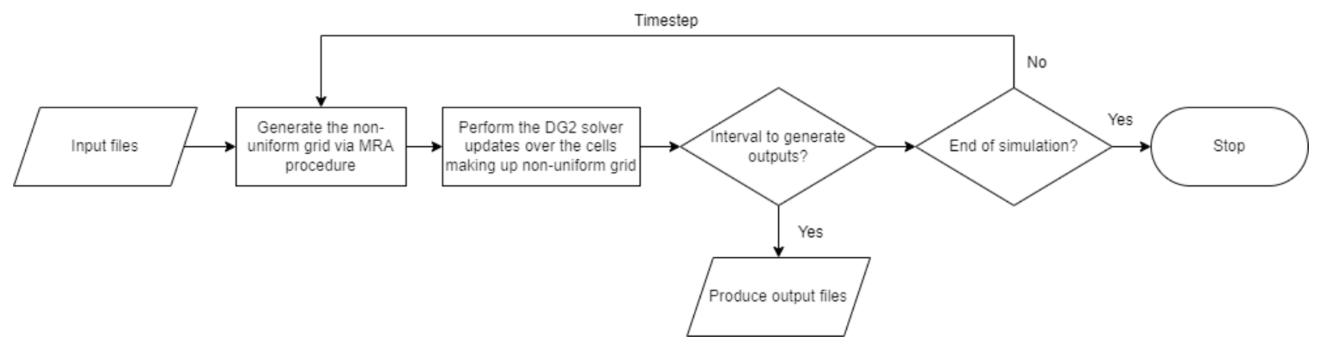
Figure 1The main operations involved in the GPU-MWDG2 solver (further detailed in Appendix A).
The technical description of the GPU-MWDG2 solver has been reported in previous papers (Kesserwani and Sharifian, 2020, 2023), whose dynamic adaptivity has here been further computationally optimised to improve memory coalescing and occupancy in the CUDA kernels (CUDA C++ Programming Guide, 2023). Therefore, the GPU-MWDG2 solver is briefly overviewed in Appendix A, with a focus on its operational workflow with reference to Fig. 1. In what follows, the presentation is focussed on describing the features incorporated into LISFLOOD-FP 8.2 for running the GPU-MWDG2 solver (Sect. 2.1), on identifying the upper limits of its GPU memory consumption in relation to the specification of the GPU card (Sect. 2.2), and on proposing metrics for detailed analysis of the efficiency of its dynamic adaptivity from output datasets (Sect. 2.3).
2.1 The GPU-MWDG2 solver
Running a simulation of a test case using any solver in LISFLOOD-FP requires setting up several test case-specific input files (https://www.seamlesswave.com/Merewether1, last access: 30 November 2025). The same is required for the GPU-MWDG2 solver (https://www.seamlesswave.com/Adaptive, last access: 30 November 2025). An important input file is the “parameter” file with the extension .par, which is a text file specifying various solver and simulation parameters (https://www.seamlesswave.com/Merewether1-1.html, last access: 30 November 2025; https://github.com/al0vya/gpu-mwdg2, last access: 30 November 2025). In the remainder of this paper, the usability of the GPU-MWDG2 solver will be described for the “Monai valley” test case (explored in Sect. 3.1) without loss of generality. Step-by-step instructions on how to use the GPU-MWDG2 solver to run a simulation of the “Monai valley” test case have been provided in Appendix B.
The parameters or keywords that should be typed in the .par file for running a simulation of the Monai Valley test case are shown in Fig. 2, including seven keywords related to running the GPU-MWDG2 solver highlighted in bold. The cuda keyword should be typed to access the GPU parallelised models in LISFLOOD-FP, e.g. the GPU-DG2 solver or the GPU-MWDG2 solver. The mwdg2 keyword should be typed to select the GPU-MWDG2 solver1. The epsilon keyword should be followed by a numerical value, e.g. 0.001 specifies the error threshold ε = 10−3. The max_ref_lvl keyword followed by an integer value specifies the maximum refinement level L, which is specified according to the DEM size and resolution, as explained next.
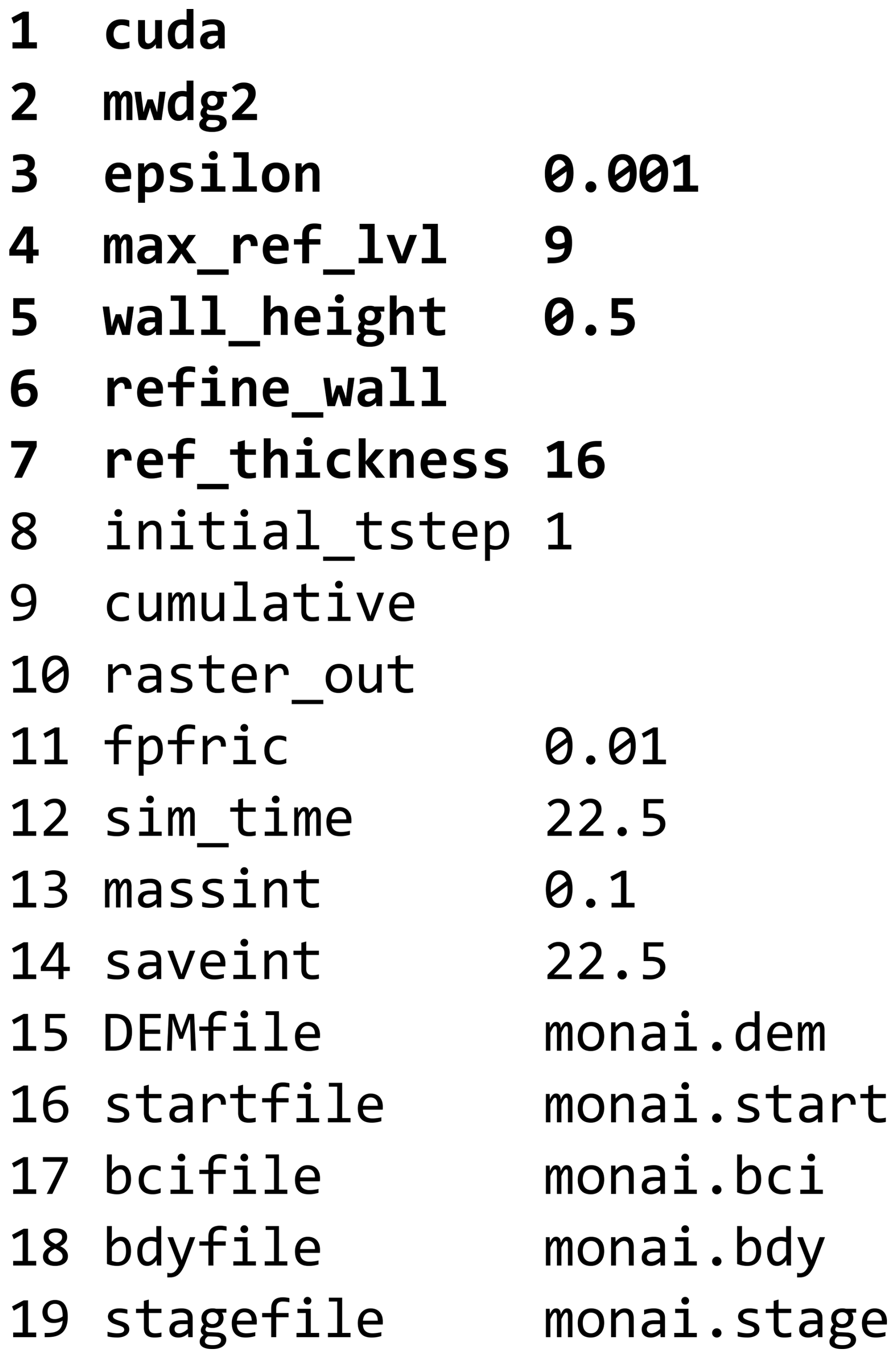
Figure 2Listing of parameters in the .par file needed to run a GPU-MWDG2 simulation for the “Monai Valley” test case (Sect. 3.1), with the GPU-MWDG2 specific items highlighted in bold.
The GPU-MWDG2 solver starts a simulation on a square uniform grid made up of 2L × 2Lcells, which is the finest-resolution grid accessible to the GPU-MWDG2 solver (Appendix A). In practice however, the DEM may often involve a (rectangular) grid with M rows and N columns, for which the GPU-MWDG2 solver still generates a starting square uniform grid with 2L × 2Lcells. A suitable choice for L is a value such that . For example, in the Monai valley test case, N = 784 and M = 486, leading to L = 10. Figure 3 shows the initial non-uniform grid generated by the GPU-MWDG2 solver. Since the GPU-MWDG2 solver starts from a square uniform grid inclusive of the DEM dimensions, two areas emerge in the non-uniform grid: the actual test case area containing the flow domain, which includes the DEM data and the initial flow conditions; and, empty areas where no DEM data are available and where no flow should occur.
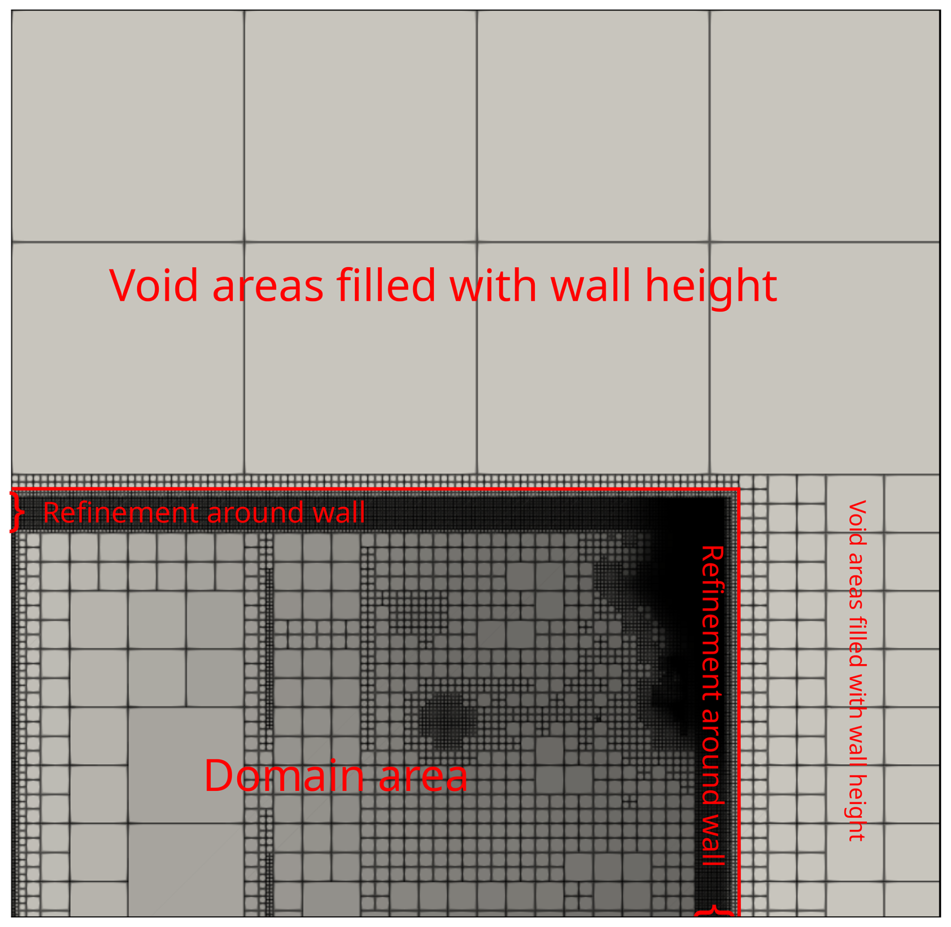
Figure 3Initial non-uniform grid generated by the GPU-MWDG2 solver, via the MRA procedure, based on the time-invariant features the DEM for the “Monai Valley” test case (Sect. 3.1).
In the actual test case area, GPU-MWDG2 initialises the data in the cells by using the values specified in .dem and .start files in raster grid format (see Appendix B). Meanwhile, in the empty areas, it initialises the flow data to zero and assigns bathymetry data the numerical value that follows the wall_height keyword. This numerical value must be sufficiently high such that a high wall is generated between the test case area and the empty areas (see Fig. 3) to prevents any water from leaving the test case area (e.g. by choosing a numerical value that is higher than the largest water surface elevation). For example, for the Monai valley test case, the wall_height keyword is specified to 0.5 m to generate a wall that is high enough to prevent any water from leaving the flow domain. The refine_wall and ref_thickness keywords, followed by an integer for the latter, typically between 16 and 64, should also be typed in the parameter file to prevent GPU-MWDG2 from excessively coarsening the non-uniform grid around the walls within the flow domain (labelled with the curly braces in Fig. 3). This prevents very coarse cells in the empty areas, covered by user-added artificial topography, from being next to very fine cells in the actual areas, covered by actual DEM topography, that could otherwise cause unphysical predictions. For the Monai valley test case, the refine_wall keyword is specified to trigger refinement around the wall, and ref_thickness is specified as 16 to trigger 16 cells at the highest refinement level between the wall and the test case area.
The remaining keywords in Fig. 2 are standard for running simulations using LISFLOOD-FP and were described previously. Note that running GPU-MWDG2 on LISFLOOD-FP 8.2 only requires the user to provide the .dem file and .start files – unlike the DG2 solvers in LISFLOOD-FP 8.0 (Shaw et al., 2021) and the static non-uniform grid generator in LISFLOOD-FP 8.1 (Sharifian et al., 2023), which require manual pre-processing of .dem1x, .dem1y, .start1x and .start1y raster files of initial DG2 slope coefficients. In the GPU-MWDG2 solver these coefficients are automatically pre-processed from the raw the .dem and .start files.
Compared to a GPU-DG2 simulation, a GPU-MWDG2 simulation consumes much more memory (Appendix A). As shown in Sect. 2.2, the large memory costs arise from the need to store the objects involved in the GPU-MWDG2 algorithm. Practically, the largest allowable choice of L or, in other words, the largest square uniform grid that can accommodate a DEM, is restricted by the memory capacity of the GPU card on which the GPU-MWDG2 simulation is performed.
2.2 GPU memory cost analysis, limits and scalability
The scope for running a GPU-MWDG2 simulation depends on the availability of a GPU card that can fit the memory costs for the specified choice of L. The left panel in Fig. 4 shows the percentage breakdown of the memory consumed by the objects involved in GPU-MWDG2 simulations: the GPU-MWDG2 non-uniform grid, the explicitly deep-copied neighbours of each cell in the grid, and the hierarchy of grids involved in the dynamic GPU-MWDG2 adaptivity process (overviewed in Appendix A). It can be seen that 15 % of the memory is allocated for arrays that store the shape coefficients of the cells in the hierarchy of uniform grids, while another 6 % is allocated for other miscellaneous purposes. Remarkably however, nearly 80 % of the overall GPU memory costs come from elsewhere: 22 % from arrays storing the shape coefficients of the cells comprising the non-uniform grid, and 57 % from arrays storing explicit deep-copies of the neighbouring shape coefficients of each cell (i.e. north, east, south, west). This high memory consumption using deep-copies ensures coalesced memory access when computing the DG2 solver updates (Appendix A). Furthermore, the GPU-MWDG2 solver is coded to allocate GPU memory for the worst-case scenario where there is no grid coarsening at all, thereby negating the need for memory reallocation after any coarsening to maximise the efficiency of dynamic GPU-MWDG2 adaptivity, since memory allocation is a relatively slow operation.
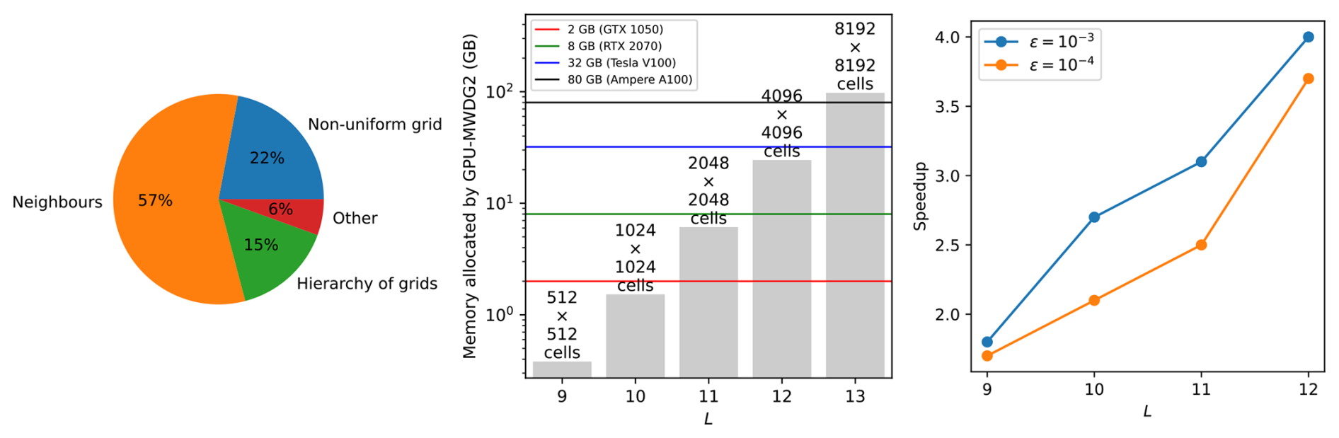
Figure 4GPU memory consumed by dynamic GPU-MWDG2 adaptivity. Left panel shows the percentage breakdown of the GPU memory consumed by the different objects involved in the GPU-MWDG2 solver. Middle panel shows the amount of GPU memory allocated against the maximum refinement level L; the numbers on top of the bars show the number of cells for a given value of L. The horizontal lines indicate the memory limits of four GPU cards. Right panel shows the scalability of the GPU-MWDG2 solver (i.e. an increasing speedup against an increasing workload) by running GPU-MWDG2 and GPU-DG2 simulations against increasing values of L for the “Monai valley” test case (Sect. 3.1) and plotting the speedups of the GPU-MWDG2 simulations compared to the GPU-DG2 simulations.
The middle panel in Fig. 4 displays the GPU memory allocated by the GPU-MWDG2 simulations for different L leading to 2L × 2Lcells on the square uniform grid. The coloured lines represent the memory limits of four different GPU cards. In this figure, the memory limits are considered for L ≥ 9, i.e. for the case where (multi)wavelet-based adaptive simulations were shown to start offering speedups over the uniform-grid simulations (Chowdhury et al., 2023; Kesserwani and Sharifian, 2023). As can be seen, dynamic GPU-MWDG2 adaptivity can only allocate GPU memory below the upper memory limit of the GPU card under consideration, leading to a restriction on the value of L that can be employed. For instance, a GTX 1050 card with a memory capacity of 2 GB can only accommodate GPU-MWDG2 simulations up to L = 10, i.e. starting from a square uniform grid made of 1024 × 1024 cells; this is because any value of L>10 will lead to exceeding this GPU card's memory limit. Generally, the larger the value of L, the larger the 2L × 2Lcells on the square uniform grid, thus the larger the memory requirement for the GPU card. At the time this study was conducted, GPU-MWDG2 simulations involving L≥13, i.e. starting from a square uniform grid from 8192 × 8192 cells, were not feasible because accommodating such values of L needed > 80 GB of GPU memory, which was higher than the memory limit of the latest commercially available GPU card (i.e. the A100 GPU card, with 80 GB of memory).
The right panel of Fig. 4 shows speedups of GPU-MWDG2 simulations over GPU-DG2 simulations with respect to L for the “Monai valley” example (Sect. 3.1) to assess the scalability of the GPU-MWDG2 solver in relation to the simulated problem size (defined by L) for the selected A100 GPU card. It can be seen that the larger the simulated problem size, the higher and steeper the speedup. This indicates that the GPU-MWDG2 solver exhibits better scalability potential with increasing size of the simulated problem, such as coupled urban and river flooding over a very large area, requiring L≥13.
2.3 Proposed metrics for analysing GPU-MWDG's runtime efficiency
Assessing the speedup that could be afforded by GPU-MWDG2 adaptivity over a GPU-DG2 simulation is essential. As noted in other works that explored wavelet adaptivity, the computational effort and speedup of a GPU-MWDG2 simulation should ideally correlate with the number of cells in the GPU-MWDG2 non-uniform grid. This correlation is expected since the number of cells dictates the number of DG2 solver updates to be performed. However, this rarely occurs in practice as the ideal speedup is diminished by the additional computational effort spent by GPU-MWDG2 in generating the non-uniform grid every timestep via the MRA process (Chowdhury et al., 2023; Kesserwani et al., 2019; Kesserwani and Sharifian, 2020, 2023). To practically assess the potential speedup of a GPU-MWDG2 simulation, one must consider the interdependent effects of the number of cells in the non-uniform grid, the computational effort of performing the DG2 solver updates, and the computational effort of performing the MRA process.
Table 1Time-dependent metrics for evaluating the potential speedup of a GPU-MWDG2 simulation over a GPU-DG2 simulation.
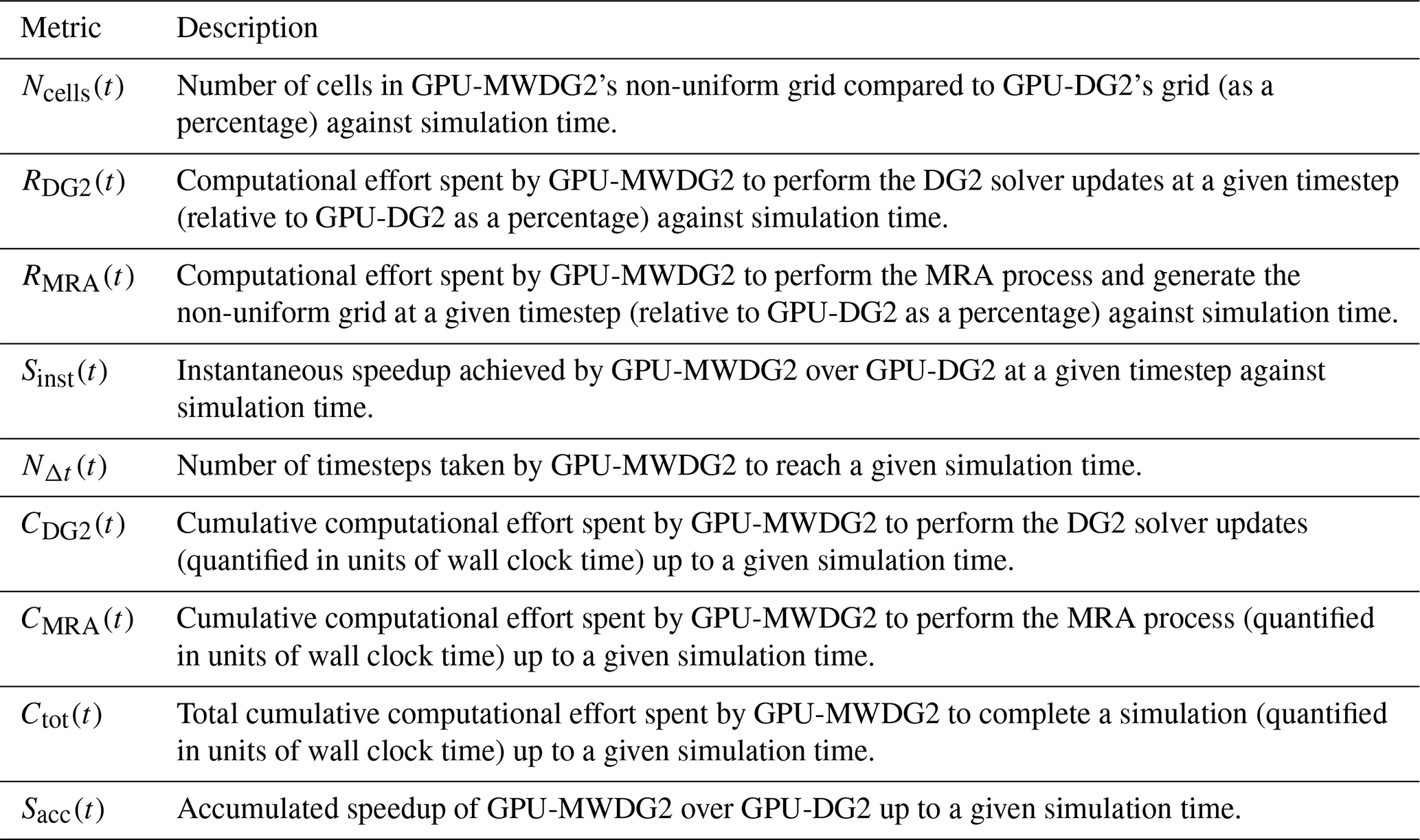
To do so, starting from LISFLOOD-FP 8.2, the user can include the cumulative keyword in the parameter file to produce a cumu file that contains the time histories of several quantities for analysing the speedup achieved by GPU-MWDG2 adaptivity. This file contains time series of the number of cells in the non-uniform grid, the computational effort of performing the DG2 solver updates per timestep, the timestep size, the timestep count, amongst other items, with the full list of items detailed in the data and script files in Chowdhury (2024). In this paper, the time histories of these quantities are postprocessed into several time-dependent metrics for analysing the speedups of GPU-MWDG2 simulations compared to GPU-DG2 simulations (Sect. 3). The metrics are described in Table 1, and their use for analysing the speedup of a GPU-MWDG2 simulation is explained next based on the Monai Valley example (Sect. 3.1).
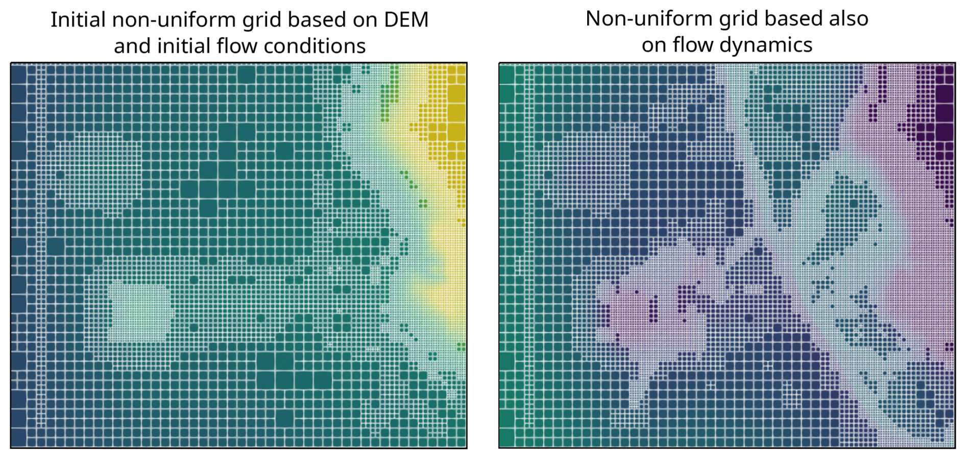
Figure 5GPU-MWDG2 non-uniform grids generated for the “Monai Valley” test case (Sect. 3.1). Left panel shows the grid at the start of the simulation whereas the right panel shows the grid after the simulation has progressed by 17 s, which tracks flow dynamics.
In a GPU-MWDG2 simulation of an impact event, the computational effort per timestep changes depending on the change in the number of cells in the GPU-MWDG2 non-uniform grid. The number of cells changes over time because finer cells are generated by GPU-MWDG2 adaptivity to track the flow features produced by the impact event as it enters and travels through the bathymetric area. The left panel of Fig. 5 shows the initial non-uniform grid generated by GPU-MWDG2 at the start of the simulation, while the right panel shows an intermediate non-uniform grid generated by GPU-MWDG2 after the simulation has progressed by 17 s, i.e. after an impact event, here a tsunami, has entered and propagated through the bathymetric area. At the start of the simulation, the initial non-uniform grid is coarsened as much as allowed, based only on the static features of the bathymetric area and initial flow conditions, leading to a minimal number of cells in the grid, which is quantified by Ncell. The number of cells determines the number of DG2 solver updates to be performed at a given timestep, leading to a corresponding computational effort per timestep, which is quantified by RDG2. There is also the computational effort of performing the MRA process at a given timestep, which is quantified by RMRA. Based on the combined computational effort of performing both the MRA process and the DG2 solver updates at a given timestep, the instantaneous speedup in completing one timestep of a GPU-MWDG2 simulation (relative to the GPU-DG2 simulation) can be computed, which is quantified by Sinst. In Fig. 5, after the simulation has progressed by 17 s, the number of cells in the non-uniform grid has increased due to using finer cells to track the tsunami's wavefronts and wave diffractions, which leads to a higher value of Ncell and RDG2 (and possibly also to a higher value of RMRA, as a higher number of cells in the non-uniform grid means more cells must be processed during the MRA process); thus, Sinst is expected to drop. Generally, the higher the complexity of the impact event, the higher the number of cells in the GPU-MWDG2 non-uniform grid, and the lower the potential speedup.
The metrics Ncell, RDG2, RMRA and Sinst quantify the computational effort and speedup of a GPU-MWDG2 simulation per timestep compared to a GPU-DG2 simulation. However, the overall or cumulative computational effort and speedup of a GPU-MWDG2 simulation depends on having accumulated the computational effort and speedup per timestep from all the timesteps taken by GPU-MWDG2 to reach a given simulation time. The higher the number of timesteps taken by GPU-MWDG2 to reach a given simulation time (quantified by NΔt), the higher the cumulative computational effort spent by GPU-MWDG2 to reach that simulation time (quantified by Ctot). The Ctot metric is computed by summing the cumulative computational effort spent by GPU-MWDG2 to perform the DG2 solver updates and the MRA process, which is quantified by CDG2 and CMRA, respectively. Using the cumulative metrics, the overall speedup accumulated by a GPU-MWDG2 simulation can be computed, which is quantified by Sacc. The metrics in Table 1 are used in the next section (Sect. 3) to assess the speedup afforded by GPU-MWDG2 adaptivity over the GPU-DG2 simulation.
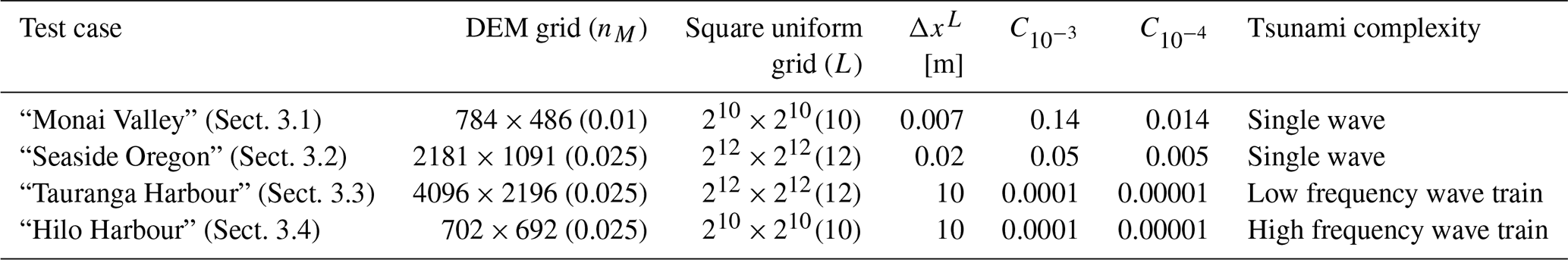
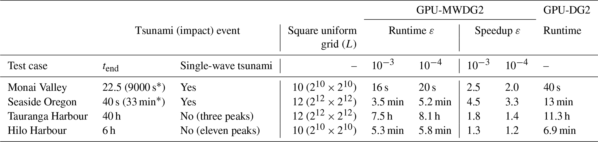
The efficiency of the GPU-MWDG2 solver is evaluated relative to the GPU-DG2 solver – which is always run on the DEM grid – using the metrics proposed in Table 1. The potential speedup afforded by GPU-MWDG2 adaptivity is hypothesised to depend on the duration and complexity of the impact event (Sect. 2.3) as well as the available DEM grid size, which dictates the choice for the L (Sect. 2.1). Therefore, the evaluation is performed by simulating four realistic test cases of tsunami-induced flooding with various impact event complexity, ranging from a single-wave to wave-train tsunamis, and DEM sizes, requiring L = 10 or 12 for the square uniform grid. The properties of the selected test cases are summarised in Table 2. The simulations were run on the Stanage high performance computing cluster of the University of Sheffield using an A100 GPU card with 80 GB of memory to accommodate the memory cost of using L=12 (see Sect. 2.2).
Table 2Information per test case. Size of N×M DEM grid and Manning coefficient nM, size of square uniform grid to accommodate the DEM grid and the associated value of L, ΔxL the resolution of the DEM grid, Cε the ratio between the smallest and largest length scale that can be captured in a simulation using a given value of ε and the ΔxL available, and the tsunami complexity.
The GPU-MWDG2 simulations are run with ε = 10−4 and 10−3, which is the range of ε where the predictive accuracy of the GPU-DG2 simulations can be preserved while achieving considerable speedups (Kesserwani and Sharifian, 2020, 2023). Here, the practical usability of these ε values is also validated based on the heuristic rule that ε should be proportional to ΔxL multiplied by a scaling factor Cε (Caviedes-Voullième et al., 2020); where, ΔxL is the (finest) resolution of the DEM grid and Cε represents the ratio between the smallest and largest length scale that can be captured during a simulation. For example, using ε = 10−3 and 10−4 in the Monai Valley test case with the available grid resolution ΔxL=0.007 yields and , respectively, which are the highest length-scale ratios that can be captured in these simulations. Similarly, and were estimated for the other test cases based on the best available DEM resolutions, and they are listed in Table 2.
According to Gerhard et al. (2015) and Gerhard and Müller (2016), a selected ε is valid if two conditions are met:
- i.
the “full error” (FE) (the error between the GPU-MWDG2 predictions and the analytical solution) is in the same order of magnitude as the “discretisation error” (DE), i.e. the error between the GPU-DG2 predictions and the analytical solution; and
- ii.
the “perturbation error” (PE) (the error between the GPU-MWDG2 and GPU-DG2 predictions) decreases by one order of magnitude when ε is also reduced by one order of magnitude for smooth numerical solutions.
In the present work, conditions (i) and (ii) can be approximately evaluated at observation points where measured data are available – to confirm the validity of ε = 10−3 and 10−4 – by quantifying FE, DE and PE, which were calculated using the root mean squared error (RMSE):
where Nobs is the number of observation points and , and are the ith observation point, GPU-DG2 prediction and GPU-MWDG2 prediction respectively. The predictions may be any of the prognostic variables, to include water surface elevation h+z or the u or v components of the velocity, or velocity-related variables.
3.1 Monai Valley
This test case has been used to validate many hydrodynamic solvers (Caviedes-Voullième et al., 2020; Kesserwani and Liang, 2012; Kesserwani and Sharifian, 2020; Matsuyama and Tanaka, 2001). It involves a 1 : 400 scaled replica of the 1993 tsunami that flooded Okushiri Island after a wave runup of 30 m at the tip of a very narrow gulley in a small cove at Monai Valley (Liu et al., 2008). The scaled DEM has 784 × 486 cells for which its associated initial square uniform grid is generated with L = 10.
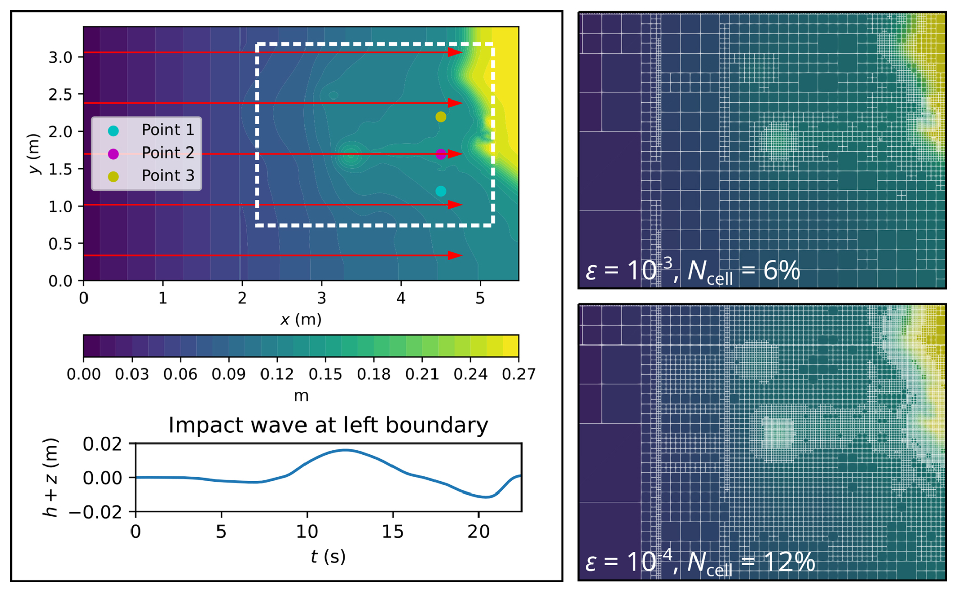
Figure 6Monai Valley. Top-down view of bathymetry (top left panel), where the red arrows indicate the direction and distance travelled by the tsunami; time history of the tsunami entering from the left boundary (bottom left panel); initial GPU-MWDG2 non-uniform grids (right panels) covering the portion of the bathymetric area framed by the white box (top left panel).
In Fig. 6, a top-down view of the bathymetric area is shown (top left panel), which has a small island in the middle and a coastal shoreline to the right, including Okushiri Island and Monai Valley. The coastal shoreline gets flooded by a tsunami that initially enters the bathymetric area from the left boundary and then travels to the right by 4.5 m (indicated by the red arrows), interacting with the small island as it travels through the bathymetric area. This tsunami is simulated for 22.5 s, during which it travels through the bathymetric area in three stages of flow over time: the entry stage (0 to 7 s), the travelling stage (7 to 17 s) and the flooding stage (17 to 22 s). During the entry stage, the tsunami does not enter the bathymetric area, as seen in the hydrograph of the tsunami's water surface elevation (bottom left panel of Fig. 6). During the travelling stage, the tsunami enters from the left boundary and travels right towards the coastal shoreline. Lastly, during the flooding stage, the tsunami floods the coastal shoreline, due to which many flow dynamics such as wave reflections and diffractions are produced that must be tracked using finer cells, thus increasing the number of cells in the GPU-MWDG2 non-uniform grid. In the right panels of Fig. 6, the initial GPU-MWDG2 grids at ε = 10−3 and 10−4 are depicted for the portion of the bathymetric area framed by the white box (top left panel of Fig. 6). With ε = 0−3 and 10−4, the initial GPU-MWDG2 grid has 6 % and 12 % of the number of cells as in the GPU-DG2 uniform grid, respectively.
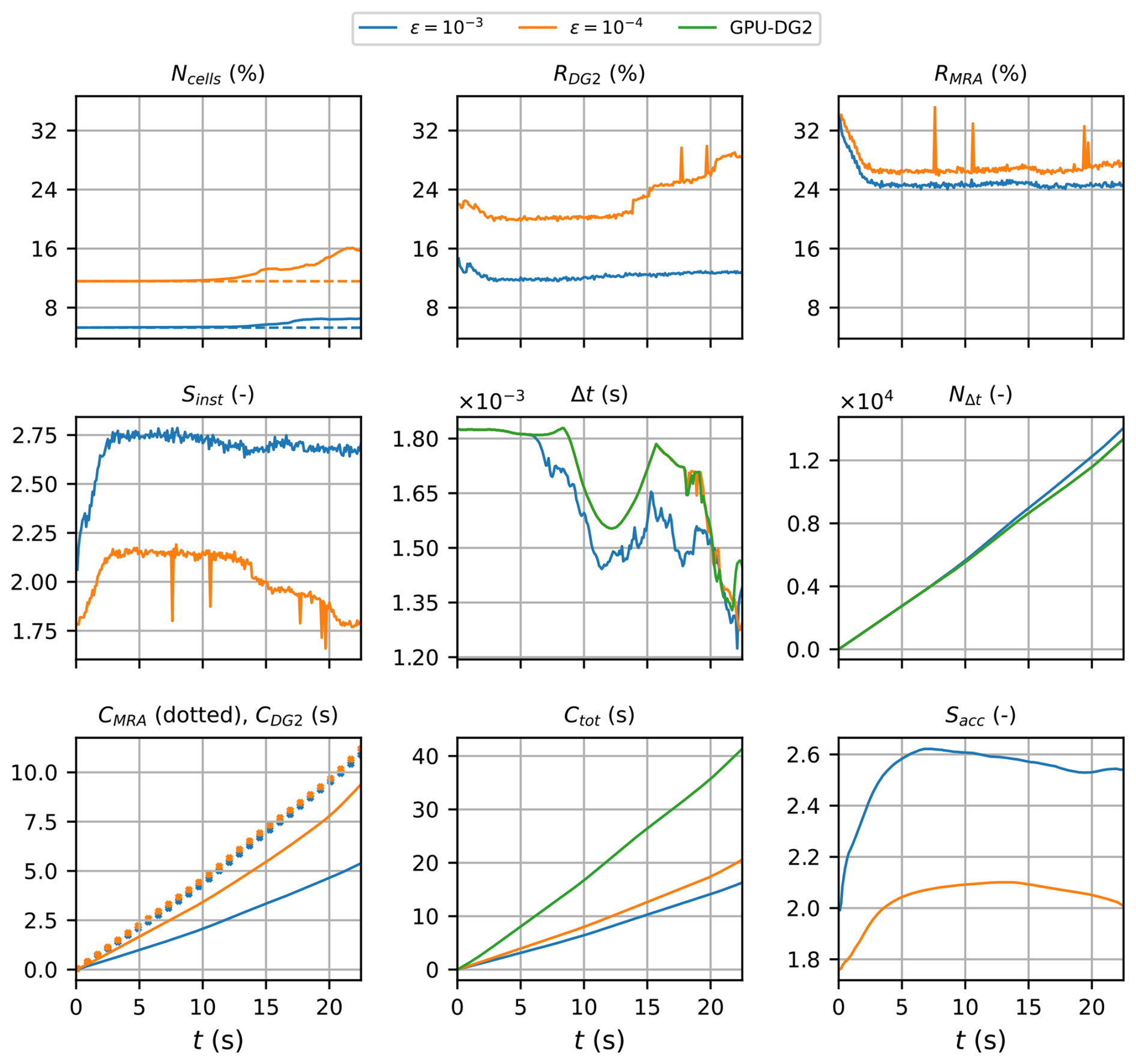
Figure 7Monai Valley. Measuring the computational performance of the GPU-MWDG2 and GPU-DG2 simulations using the metrics of Table 1 to assess the speedup afforded by GPU-MWDG2 adaptivity: Ncells, the number of cells in the GPU-MWDG2 non-uniform grid,where the dashed line represents the initial value at the beginning of the simulation; RDG2,the computational effort of performing the DG2 solver updates at given timestep relative to the GPU-DG2 simulation; RMRA, the relative computational effort of performing the MRA process at a given timestep; Sinst, the instantaneous speedup achieved by the GPU-MWDG2 simulation over the GPU-DG2 simulation at a given timestep; Δt, the simulation timestep; NΔt, the number of timesteps taken to reach a given simulation time; CDG2, the cumulative computational effort of performing the DG2 solver updates up to a given simulation time; CMRA, the cumulative computational effort of performing the MRA process; Ctot, the total cumulative computational effort; Sacc, the accumulated speedup of GPU-MWDG2 over GPU-DG2 up to a given simulation time.
In Fig. 7, an analysis of the runtimes of the GPU-DG2 and GPU-MWDG2 simulations using the time-dependent metrics of Table 1 is shown. Up to 15 s, i.e. before the flooding stage of flow begins, the time history of Ncell remains flat, meaning that the number of cells in the GPU-MWDG2 non-uniform grid does not change over time. Once the flooding stage begins however, Ncell increases slightly, particularly at ε = 10−4. With an increased number of cells in the non-uniform grid, the computational effort of performing the DG2 solver updates per timestep should increase, as is confirmed by the time history of RDG2, which is flat before the flooding stage of flow, but thereafter increases, particularly at ε = 10−4. However, unlike RDG2, the time history of RMRA is similar for both values of ε, and stays flat for most of the simulation except for an initial decrease at the start, meaning that the computational effort of performing the MRA process per timestep is similar for both values of ε and remains fixed throughout the simulation. Thus, the drop in the speedup of completing a single timestep of the GPU-MWDG2 simulation compared to the GPU-DG2 simulation is mostly due to the increase in RDG2 at ε = 10−4, with Sinst dropping from 2.0 to 1.8 (which otherwise stays flat at 2.7 for ε = 10−3).
The cumulative computational effort is affected by the timestep size (Δt) and the number of timesteps taken to reach a given simulation time (NΔt). In this test case, the time histories of Δt of the GPU-DG2 simulation and the GPU-MWDG2 simulation using ε = 10−4 are very similar, but with ε = 10−3, it drops at 7 s, i.e. as soon as the travelling stage of flow begins. This slight drop in Δt is likely caused by the existence of planar DG2 solutions per cell with either partially wet portions or thin water layers under friction effects that locally and temporarily triggers smaller-scale timesteps. Either of these are more likely to be present in coarser cells, thereby reducing Δt with ε = 10−3. Due to the smaller Δt at ε = 10−3, the trend in NΔt is steeper at ε = 10−3 than 10−4, i.e. more timesteps are taken and thus more computational effort is spent by GPU-MWDG2 to reach a given simulation time at ε = 10−3 than 10−4. Still, despite the steeper trend in NΔt, the cumulative computational effort of performing the MRA process is similar using both ε = 10−3 and 10−4, which is expected given that RMRA is also very similar for values of ε. In contrast, the cumulative computational effort of performing the DG2 solver updates is considerably higher at ε = 10−4 than 10−3, likely due to the higher RDG2 at ε = 10−4, which seems correct since a higher computational effort to perform the DG2 solver updates per timestep should lead to a higher cumulative computational effort (assuming that the time histories of NΔt are similar for the different values of ε, which is the case here). Notably though, CDG2 is actually smaller than CMRA, meaning that in this test case, the computational effort is dominated by the MRA process rather than the DG2 solver updates. Overall, for both values of ε, the total computational effort of running the GPU-MWDG2 simulations is always lower than that of the GPU-DG2 simulation, with Ctot always being lower than that of GPU-DG2 at both ε = 10−3 and 10−4. The accumulated speedups of the GPU-MWDG2 simulations, Sacc, finish at around 2.5 and 2.0 using ε = 10−3 and 10−4, respectively.
Table 3Monai valley. DE, FE and PE quantified using Eqs. (1) to (3) considering measured and predicted time series of the water surface elevation at points 1, 2 and 3 in Fig. 7. The errors are computed in order to check for fulfilment of conditions (i) and (ii) and to confirm the validity of selecting ε = 10−3 and 10−4 in this test case.
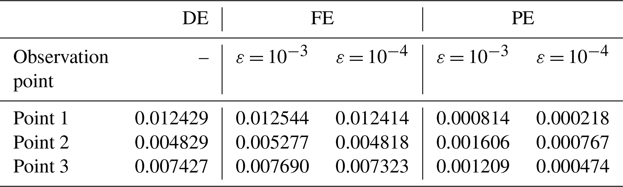
In Fig. 8, the GPU-MWDG2 predictions at ε = 10−3 and 10−4 and the GPU-DG2 prediction of the water surface elevation h+z at points 1, 2 and 3 (i.e. the coloured points in the top left panel of Fig. 7) are shown. All three predictions are very similar to each other visually, although at point 2, the wave arrival time is seen to be slightly underpredicted using ε = 10−3. In Table 3, the FE, DE and PE at the same points are shown: the FE and DE are of the same order of magnitude, while the PE decreases by around an order of magnitude since the simulation does not involve strong discontinuities. This shows fulfilment of conditions (i) and (ii), in turn confirming the validity of the selected ε values in this test case.
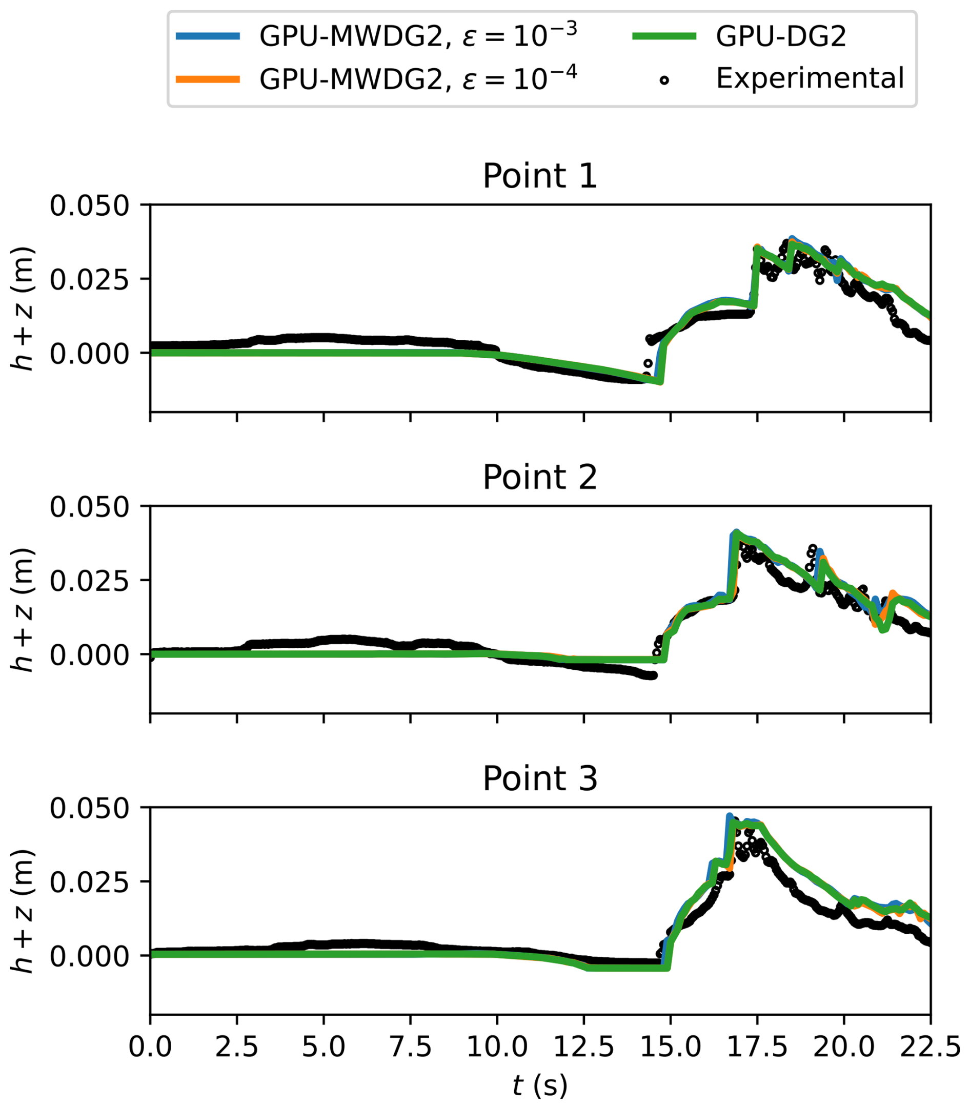
Figure 8Monai Valley. Time series of the water surface elevation (h+z) predicted by GPU-DG2 and GPU-MWDG2 at the three sampling points (shown in Fig. 6, top left panel) compared to the experimental results.
Overall, the GPU-MWDG2 solver closely reproduces the GPU-DG2 water surface elevation predictions while being two times faster than the GPU-DG2 solver due to using L = 10. This is in line with the speedups shown in Fig. 4 in Sect. 2.2, which suggests that L = 10 is the “borderline” value of L where GPU-MWDG2 adaptivity reliably yields a speedup. In the next test case, the impact of a larger DEM size – requiring a larger L value – on the speedup of the GPU-MWDG2 solver is evaluated. The prediction of more complex velocity-related quantities is also considered.
3.2 Seaside Oregon
This is another popular benchmark test case that has been used to validate hydrodynamic solvers for nearshore tsunami inundation simulations (Gao et al., 2020; Macías et al., 2020a; Park et al., 2013; Qin et al., 2018; Violeau et al., 2016). It involves a 1 : 50 scaled replica of an urban town in Seaside, Oregon that is flooded by a tsunami travelling along a scaled DEM made up of 2181 × 1091 cells, here requiring a larger L = 12 to generate the initial square uniform grid.
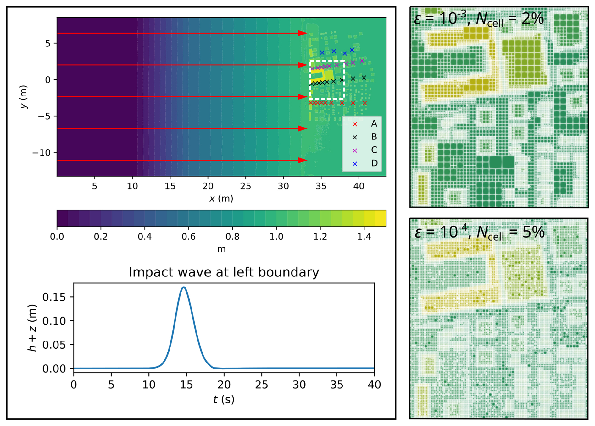
Figure 9Seaside Oregon. Top-down view of bathymetry (top left panel), where the red arrows indicate the direction and distance travelled; tsunami time history entering the left boundary (bottom left panel); initial GPU-MWDG2 grids (right panels) for the potion in white box (top left panel).
In Fig. 9, the bathymetric area is shown (top left panel), which is very flat everywhere except to the right where very complex terrain features of the urban town, such as buildings and streets, are located. The urban town is flooded by a tsunami that enters from the left boundary and travels a distance of 33 m to the right before flooding the town (as shown by the red arrows). This tsunami is simulated for 40 s, during which it travels through the bathymetric area in four stages of flow over time, much like in the last test case (Sect. 3.1): the entry stage (0 to 10 s), the travelling stage (10 to 25 s), the flooding stage (25 to 35 s) and the inundation stage (35 to 40 s). During the entry stage, the tsunami is not yet in the bathymetric area; during the travelling stage, the tsunami starts to enter the bathymetric area from the left boundary and travels right towards the town; during the flooding stage, the tsunami hits the town, flooding the streets and overtopping some of the buildings, causing vigorous flow dynamics; finally, during the inundation stage, the tsunami inundates the town and goes on to interact with the right boundary, causing wave reflections. The water surface elevation hydrograph of the tsunami is plotted in the bottom left panel of Fig. 9: it only has a single peak, therefore leading to low tsunami complexity. The right panels show the initial GPU-MWDG2 non-uniform grids at ε = 10−3 and 10−4, respectively (again for the portion of the bathymetric area framed by the white box in top left panel): at ε = 10−3, greater grid coarsening is achieved, with the grid including only 2 % of the number of cells as in the GPU-DG2 uniform grid, whereas at ε = 10−4 it is 5 % since more cells are used due to retention of finer resolution around and within complex terrain features of the urban town.
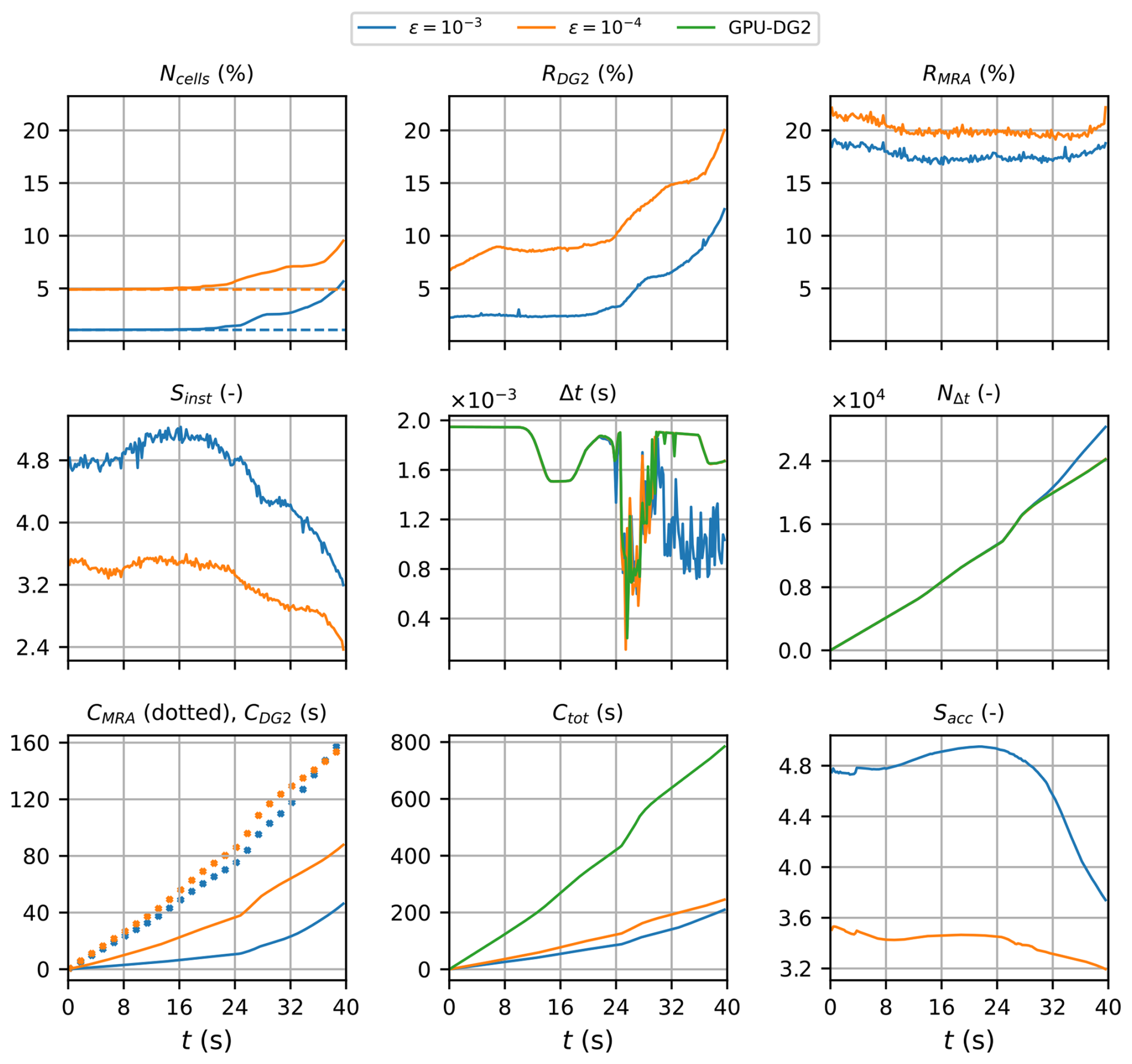
Figure 10Seaside Oregon. Measuring the computational performance of the GPU-MWDG2 and GPU-DG2 simulations using the metrics of Table 1 to assess the speedup afforded by GPU-MWDG2 adaptivity: Ncells,the number of cells in the GPU-MWDG2 non-uniform grid,where the dashed line represents the initial value at the beginning of the simulation; RDG2, the computational effort of performing the DG2 solver updates at given timestep relative to the GPU-DG2 simulation; RMRA, the relative computational effort of performing the MRA process at a given timestep; Sinst, the instantaneous speedup achieved by the GPU-MWDG2 simulation over the GPU-DG2 simulation at a given timestep; Δt, the simulation timestep; NΔt, the number of timesteps taken to reach a given simulation time; CDG2, the cumulative computational effort of performing the DG2 solver updates up to a given simulation time; CMRA, the cumulative computational effort of performing the MRA process; Ctot, the total cumulative computational effort; Sacc, the accumulated speedup of GPU-MWDG2 over GPU-DG2 up to a given simulation time.
In Fig. 10, an analysis of runtimes of the GPU-MWDG2 and GPU-DG2 simulations are shown. As indicated by the time history of Ncell, the number of cells in the GPU-MWDG2 non-uniform grid does not increase significantly for either value of ε until the flooding stage of flow at 25 s, where Ncell starts increasing more noticeably. Once the number of cells starts increasing, there is a corresponding increase in RDG2. On the other hand, the time history of RMRA is quite flat during the entire simulation, except for a small decrease during the first 10 s of the simulation, and a small increasing trend in the final 5 s of the simulation, i.e. during the inundation stage of flow when the number of cells increases relatively sharply compared to the rest of the simulation. Driven primarily by the increase in RDG2 at the flooding stage at 25 s, the time history of Sinst is quite stable until 25 s and thereafter shows a decreasing trend that is particularly steep at ε = 10−3.
Like the previous test case (Sect. 3.1), the time histories of Δt in the GPU-DG2 simulation and GPU-MWDG2 simulation at ε = 10−4 are very similar, but at ε = 10−3, there is a sharp drop in Δt after 32 s, i.e. when the flooding stage of flow starts transitioning to the inundation stage. Again, this sharp drop in Δt is triggered by coarse cells that are either partially wet or have thin water layers, which are more likely in the non-uniform grid with ε = 10−3, but not with 10−4. The first drop in Δt, which occurs at 25 s when the flooding stage starts, leads to a locally steeper trend in the time history of NΔt, as indicated by the kink in the trend at 25 s. The second drop in Δt, which is seen only for ε = 10−3 after 32 s, leads to a sustained steepness in the time history of NΔt. This steepness means that GPU-MWDG2 takes more timesteps and thus accumulates more computational effort to reach a given simulation time at ε = 10−3 than 10−4, which is confirmed by the final value of CMRA, which is higher at the end of the simulation at ε = 10−3 compared to 10−4, even though it was lower at ε = 10−3 than at ε = 10−4 for the rest of the simulation. Since RMRA is always lower at ε = 10−3 than 10−4, this observation about CMRA suggests that even if the computational effort per timestep is lower throughout the simulation, a high timestep count can sufficiently increase the cumulative computational effort such that it becomes higher at ε = 10−3 than 10−4. Nonetheless, the time history of Ctot in the GPU-MWDG2 simulations always remains well below that of the GPU-DG2 simulation, with Sinst finishing at 3.5 and 3.0 with ε = 10−3 and 10−4, respectively.
In Fig. 11, the time series predicted by GPU-MWDG2 using ε = 10−3 and 10−4 and GPU-DG2 of the prognostic variables h+z, the u component of the velocity, and the derived momentum variable Mx = 0.5hu2 at points A1, B6 and D4 are shown. Point A1 is one of the left-most crosses in Fig. 9, point B6 is one of the central crosses, and point D4 is one of the right-most crosses. At all three points, the predictions are visually similar to each other except at point D4, where, for ε = 10−3, the impact wave height is slightly overpredicted, while the velocity and momentum is overpredicted between 33 s and 43 s. Compared to the measured data, the predictions all follow the trailing part of the measurement time series quite well, but at the peaks, they are underpredicted at point A1, overpredicted at point B6, and out of phase at point D4. These differences, which manifest most noticeably at the peaks, may be due to the incoming bore of the impact wave, which had invalidated measurements and required repeating experiments, possibly introducing uncertainty into the measured data (Park et al., 2013).
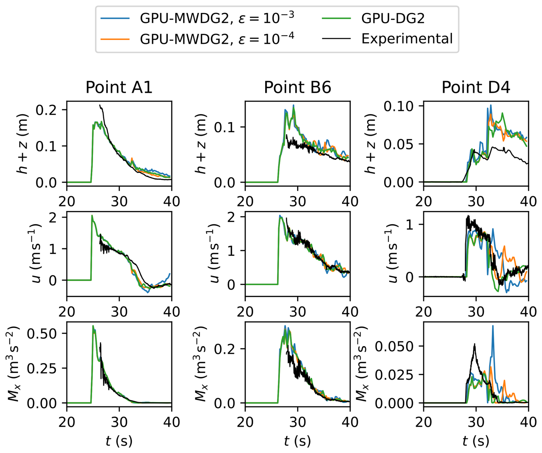
Figure 11Seaside Oregon. Time series of the water surface elevation (h+z), u velocity component and momentum Mx for the GPU-DG2 and GPU-MWDG2 predictions at points A1, B6 and D4 (Fig. 9), compared to the experimental data.
Table 4Seaside Oregon. DE, FE and PE quantified using Eqs. (1) to (3) considering measured and predicted time series of the prognostic variables h+z, u and Mx at points A1, B6 and D4 (shown in Fig. 9). The errors are considered in order to check for fulfilment of conditions (i) and (ii) and confirm the validity of selecting ε = 10−3 and 10−4 in this test case.
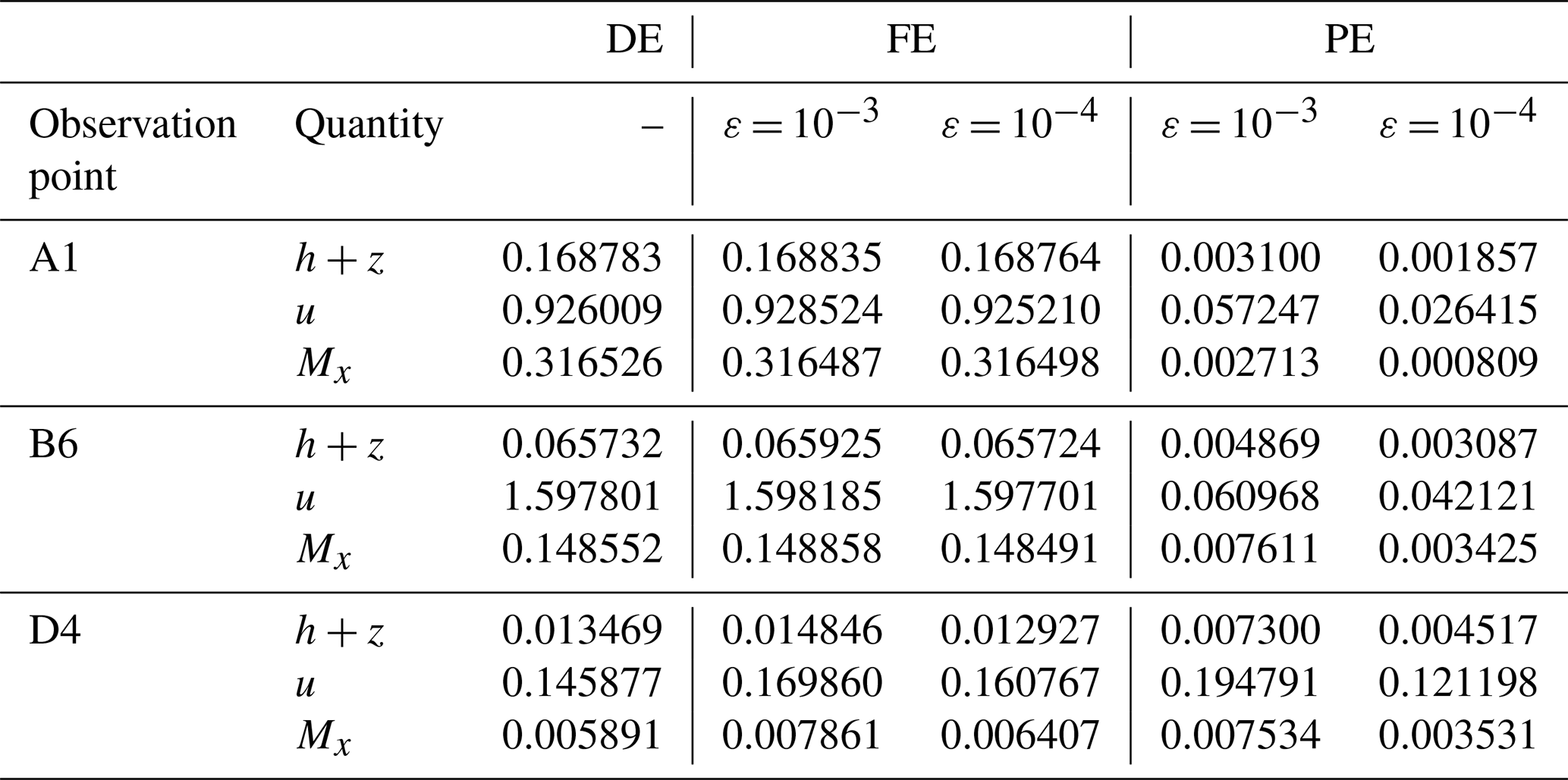
Table 4 shows the associated DE, FE and PE at points A1, B6 and D4. The errors confirm fulfilment of conditions (i) and (ii) and thus show that selected ε values are valid: the DE and FE are in the same order of magnitude, while decreasing ε from 10−3 to 10−4 leads to a reduction in the PE – although the reduction is less than an order of magnitude compared to the last test case (Sect. 3.1) due to the strong discontinuities introduced into the numerical solution by the buildings in the urban area.
This test case and the previous show that the GPU-MWDG2 solver can achieve at least a 2-fold speedup over the GPU-DG2 solver for tsunami simulations involving a single-wave impact event. Notably though, if the impact event had been present for a larger fraction of the simulation time, it would have introduced a correspondingly higher amount of complexity over time, and a higher cumulative computational effort would have been expected. This type of event will be explored next in Sect. 3.3 and 3.4.
3.3 Tauranga Harbour
This test case reproduces the 2011 Japan tsunami event in Tauranga Harbour, New Zealand (Borrero et al., 2015; Macías et al., 2015, 2020b). The bathymetric area has a DEM made of 4096 × 2196 cells, requiring L = 12 to generate the initial square uniform grid. As shown by the red arrows in Fig. 12, the tsunami enters from the top boundary and travels a short distance downwards before quickly hitting the coast at y = 16 km. As shown by the time history of the water surface elevation (bottom left panel of Fig. 12), the tsunami is a wave train made up of three wave peaks and troughs that enter that bathymetric area one after the other at 0, 12 and 24 h during the 40 h tsunami event, with the latter two waves also exhibiting noise. Vigorous flow dynamics occur within the bathymetric area from the very beginning of the simulation, due to complex impact event and the irregular bathymetric zones that trigger wave reflections and diffractions. The right panels of Fig. 6 include the GPU-MWDG2 grids generated at ε = 10−3 and 10−4 for the region bounded by the white box (top left panel). With ε = 10−3, the number of cells in the grid is 5 % of the GPU-DG2 uniform grid, whereas with ε = 10−4, it is 15 %, due to less coarsening in and around the irregular bathymetric zones.
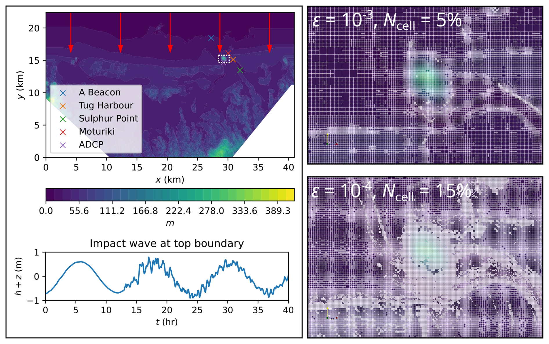
Figure 12Tauranga Harbour. Top-down view of bathymetry (top left panel), where the red arrows indicate the direction and distance travelled; tsunami time history entering the top boundary (bottom left panel); initial GPU-MWDG2 grids (right panels) for the potion in white box (top left panel).
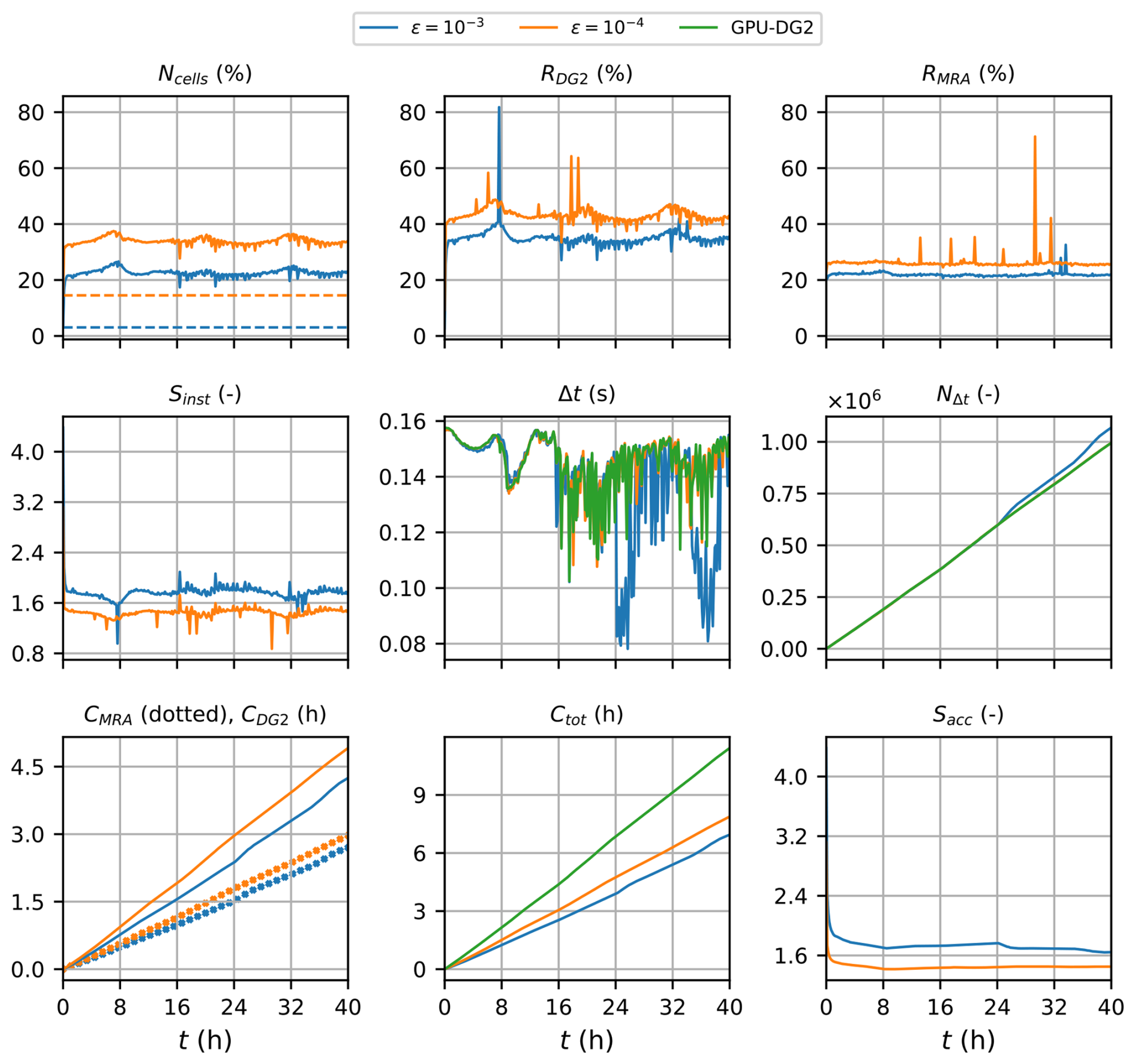
Figure 13Tauranga Harbour. Measuring the computational performance of the GPU-MWDG2 and GPU-DG2 simulations using the metrics of Table 1 to assess the speedup afforded by GPU-MWDG2 adaptivity: Ncells,the number of cells in the GPU-MWDG2 non-uniform grid,where the dashed line represents the initial value at the beginning of the simulation; RDG2, the computational effort of performing the DG2 solver updates at given timestep relative to the GPU-DG2 simulation; RMRA, the relative computational effort of performing the MRA process at a given timestep; Sinst, the instantaneous speedup achieved by the GPU-MWDG2 simulation over the GPU-DG2 simulation at a given timestep; Δt, the simulation timestep; NΔt, the number of timesteps taken to reach a given simulation time; CDG2, the cumulative computational effort of performing the DG2 solver updates up to a given simulation time; CMRA, the cumulative computational effort of performing the MRA process; Ctot, the total cumulative computational effort; Sacc, the accumulated speedup of GPU-MWDG2 over GPU-DG2 up to a given simulation time.
In Fig. 13, an analysis of the runtimes of the GPU-MWDG2 and GPU-DG2 simulations is shown. Unlike the previous test cases (Sect. 3.1 and 3.2), the first wave of the tsunami wave train enters the bathymetric immediately, causing Ncell to increase very sharply and immediately from its initial value for both values of ε, which thereafter fluctuates due to the periodic tsunami signal. Following the sharp increase and fluctuations in Ncell, RDG2 also sharply increases and fluctuates. However, RMRA does not and stays stable and flat throughout the simulation. Thus, driven primarily by the sharp decrease in RDG2, Sinst decreases sharply from 4.0 to 1.6. The time histories of Δt in the GPU-DG2 simulation and the GPU-MWDG2 simulation using ε = 10−4 follow each other quite closely up to 16 h, but at ε = 10−3, the time history of Δt shows two periodic drops after 24 h. These drops are likely due to periodic wetting and drying processes that trigger coarse cells with partially wet portions or thin water layers, which are more common in the non-uniform grid at ε = 10−3 but not at 10−4. Due to the smaller Δt at ε = 10−3, the time history of NΔt is locally steeper (see the kinks at 25 and 35 h), but this does not lead to significant differences between the cumulative computational effort at ε = 10−3 versus 10−4. The time history of Ctot in the GPU-MWDG2 simulations remains consistently below that of the GPU-DG2 simulation for both values of ε, but they are relatively close to each other compared to the previous test cases (Sect. 3.1 and 3.2). Thus, even though Sacc starts at around 4, like in the previous test case with L = 12 (Sect. 3.2), it drops sharply to 1.6 and 1.4 at ε = 10−3 and 10−4, respectively.
Table 5Tauranga Harbour. DE, FE and PE quantified using Eqs. (1) to (3) considering measured and predicted time series of the water surface elevation h+z at observation points A Beacon, Tug Harbour, Sulphur Point and Moturiki (top left panel of Fig. 12), and the speed () at observation point ADCP. The errors are considered in order to check for fulfilment of conditions (i) and (ii) and confirm the validity of selecting ε = 10−3 and 10−4 in this test case.
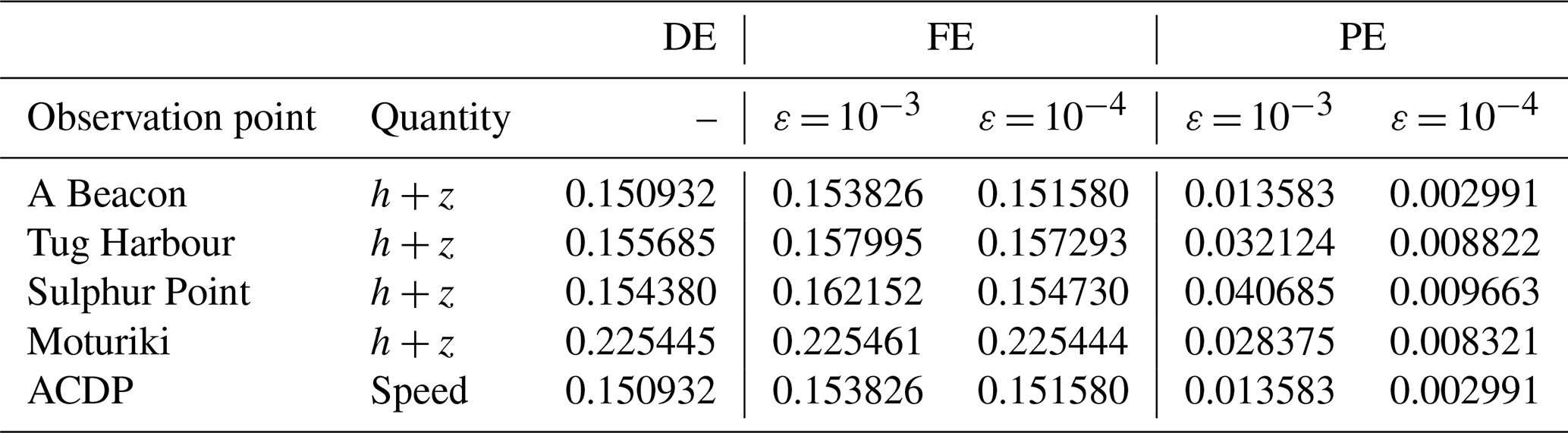
In Fig. 14, the top four panels show the time series of the water surface elevation predicted by GPU-MWDG2 using ε = 10−3 and 10−4 and by GPU-DG2 at observation points A Beacon, Tug Harbour, Sulphur Point and Moturiki (top left panel of Fig. 12). All of the predictions are visually in agreement with each other as well as the measured data. Meanwhile, the bottom panel of Fig. 14 shows the speed () predicted at observation point ADCP, where the predictions are still visually in agreement with each other, but less so with the measured speed, as was also observed for the velocity-related predictions in the last test case (Sect. 3.2). Table 5 quantifies the extent of agreement by showing the associated DE, FE and PE at the observation points. The DE and FE are in the same order of magnitude, while the PE is reduced by close to an order of magnitude when ε is decreased from 10−3 to 10−4, fulfilling conditions (i) and (ii) and thereby validating the used ε choices.
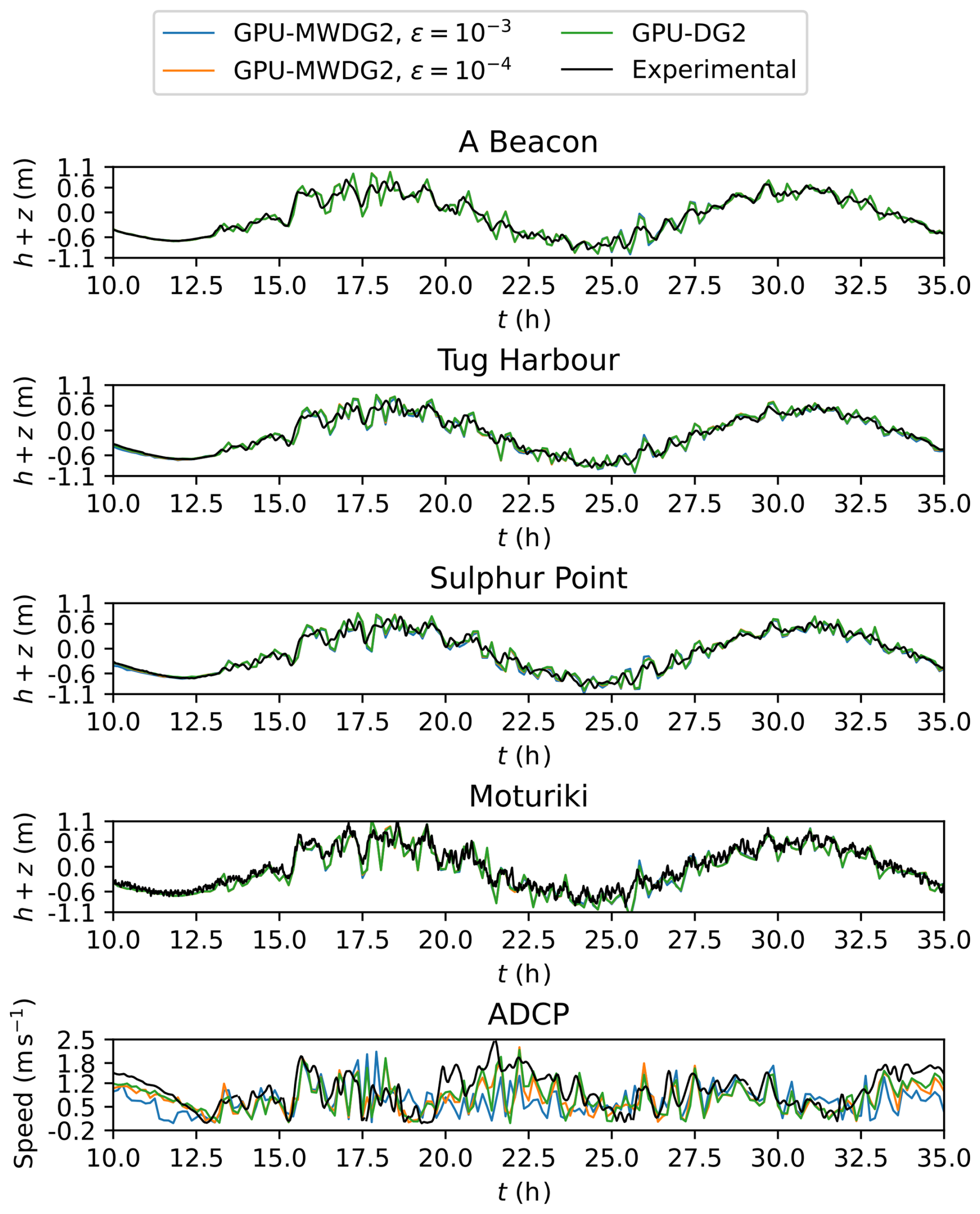
Figure 14Tauranga Harbour. Time series of the water surface elevation (h+z) produced by GPU-DG2 and GPU-MWDG2 at the points labelled A Beacon, Tug Harbour, Sulphur Point and Moturiki (labelled in Fig. 12) and for the speed () at the point ADCP (also labelled in Fig. 12), compared to the experimental results.
Overall, this test case features a more complex tsunami compared to the previous test cases (Sect. 3.1 and 3.2), which sharply increases the number of cells in the GPU-MWDG2 non-uniform grid and thus also increases the computational effort of performing the DG2 solver updates. Hence, despite requiring the same L = 12 as the previous test case (Sect. 3.2), the final speedups are lower in this test case due to the more complex tsunami, with Sacc finishing at 1.6- and 1.4-fold with ε = 10−3 and 10−4, respectively. Both choices of ε = 10−4 and 10−3 are valid for this test case: using ε = 10−4 would improve the closeness to the GPU-DG2 predicted velocities, while using ε = 10−3 leads to very close water surface elevation predictions and fairly accurate velocity predictions, although without a major improvement in the speedup. In the next test case, another complex tsunami with higher frequency impact event peaks is considered, but now with a smaller DEM size requiring L=10.
3.4 Hilo Harbour
This test case reproduces the 2011 Japan tsunami event at Hilo Harbour in Hawaii, USA (Arcos and LeVeque, 2014; Lynett et al., 2017; Macías et al., 2020b; Velioglu Sogut and Yalciner, 2019). It involves a complex tsunami made up of a high-frequency wave train that propagates for 6 h into a bathymetric area that is smaller than the previous test case (Sect. 3.3): the current bathymetric area has a DEM size made of 702 × 692 cells, requiring a smaller L = 10 to generate the initial square uniform grid. As shown in Fig. 15, the tsunami enters from the top boundary and travels south to flood the coast at y = 4 km. The wave train occurs over the entire 6 h simulation time, from a reference timestamp of 7 to 13 h post-earthquake. In Fig. 15, the time history of the wave train is shown during the 8.5 to 11 h time period (bottom left panel): from the very beginning and during the entire simulation, violent flow dynamics occur in the bathymetric area. The right panels show the initial GPU-MWDG2 non-uniform grids generated at ε = 10−3 and 10−4 for the region bounded by the white box (top left panel): the number of cells in the initial non-uniform grids are at 10.0 % and 22.5 % of the GPU-DG2 uniform grid at ε = 10−3 and ε = 10−4, respectively.
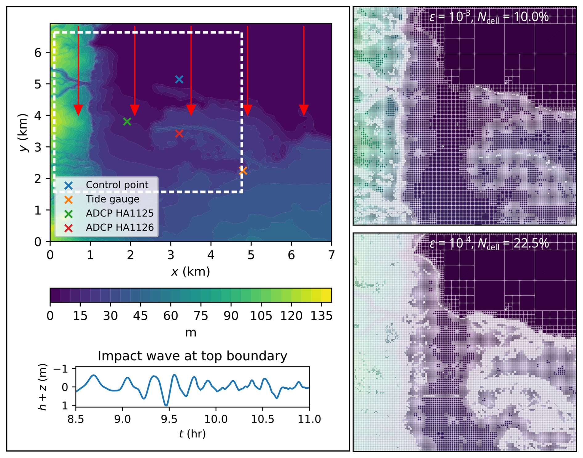
Figure 15Hilo Harbour test case. Top-down view of bathymetry (top left panel), where the red arrows indicate the direction and distance travelled; tsunami time history entering the top boundary (bottom left panel); initial GPU-MWDG2 grids (right panels) for the potion in white box (top left panel).
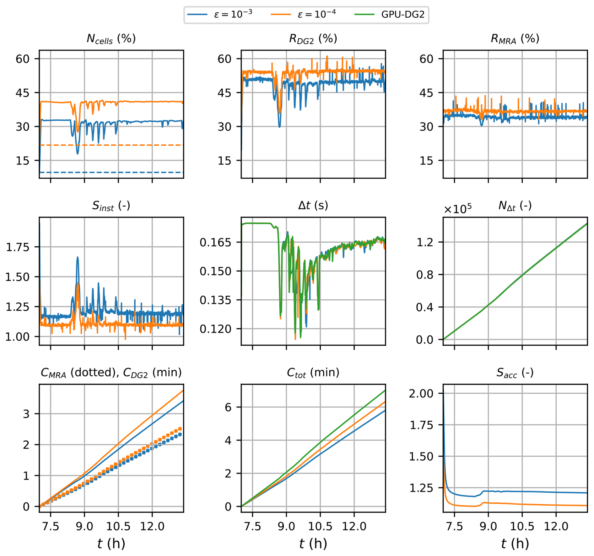
Figure 16Hilo Harbour. Measuring the computational performance of the GPU-MWDG2 and GPU-DG2 simulations using the metrics of Table 1 to assess the speedup afforded by GPU-MWDG2 adaptivity: Ncells,the number of cells in the GPU-MWDG2 non-uniform grid,where the dashed line represents the initial value at the beginning of the simulation; RDG2,the computational effort of performing the DG2 solver updates at given timestep relative to the GPU-DG2 simulation; RMRA, the relative computational effort of performing the MRA process at a given timestep; Sinst, the instantaneous speedup achieved by the GPU-MWDG2 simulation over the GPU-DG2 simulation at a given timestep; Δt, the simulation timestep; NΔt, the number of timesteps taken to reach a given simulation time; CDG2, the cumulative computational effort of performing the DG2 solver updates up to a given simulation time; CMRA, the cumulative computational effort of performing the MRA process; Ctot, the total cumulative computational effort; Sacc, the accumulated speedup of GPU-MWDG2 over GPU-DG2 up to a given simulation time.
In Fig. 16, an analysis of runtimes of the GPU-MWDG2 and GPU-DG2 simulations is shown. Like the last test case (Sect. 3.3), the wave train enters the bathymetric area immediately and Ncell increases sharply and immediately to maximum values of 32 % and 40 % at ε = 10−3 and 10−4, respectively. The time history of Ncell stays at this maximum for the rest of the simulation except for localised drops at certain simulation times, e.g. at 8 h. Following Ncell, RDG2 also increases sharply and immediately (to maximum values of 50 % and 55 % at ε = 10−3 and 10−4, respectively), and shows localised drops at the same times as the drops in Ncell. In contrast, the time history of RMRA stays very flat throughout the simulation, except for a small, temporary drop at 8 h, which is when the largest drop in Ncell occurs. Due to the generally flat time histories of RDG2 and RMRA, the time history of Sinst is also flat except for localised peaks that occur at the same times as the localised drops in RDG2 and RMRA. Unlike all of the previous test cases (Sect. 3.1–3.3), the time history of Δt is very similar between the GPU-DG2 simulation and the GPU-MWDG2 simulations, regardless of the ε value as they both yield high numbers of cells compared to the uniform GPU-DG2 grid, leading to highly refined non-uniform grids that are unlikely to have coarse cells compared to the previous test cases. Thus, the time history of NΔt is virtually identical across all simulations. Given that the time histories of NΔt, RDG2 and RMRA are similar for both ε values, the time histories of CDG2 and CMRA are also very similar, but importantly, due to the complex flows leading to highly refined non-uniform grids, the former dominates the latter in terms of the total computational effort. Overall, the time history of Ctot is very close between the GPU-DG2 simulation and the GPU-MWDG2 simulations in this test case (even more so than in the last case, Sect. 3.3), so Sacc is the lowest out of all the test cases, finishing at 1.25 and 1.10 using ε = 10−3 and 10−4, respectively.
Figure 17 shows the time series of the water surface elevation at observation points labelled “Control point” and “Tide gauge”, and the time series of the u and v velocity components at the points labelled “ADCP HA1125” and “ADCP HA1126” (top left panel in Fig. 15) predicted by GPU-DG2 using ε = 10−3 and 10−4 and GPU-MWDG2. All the predictions are visually very similar to each other except for the u prediction, where some differences are seen for ε = 10−3 and 10−4. Compared to the measured data, both agreement and differences are seen, but it may not be possible to make a confident judgment due to the sparsity in the measured data – see the jagged shape of the black line.
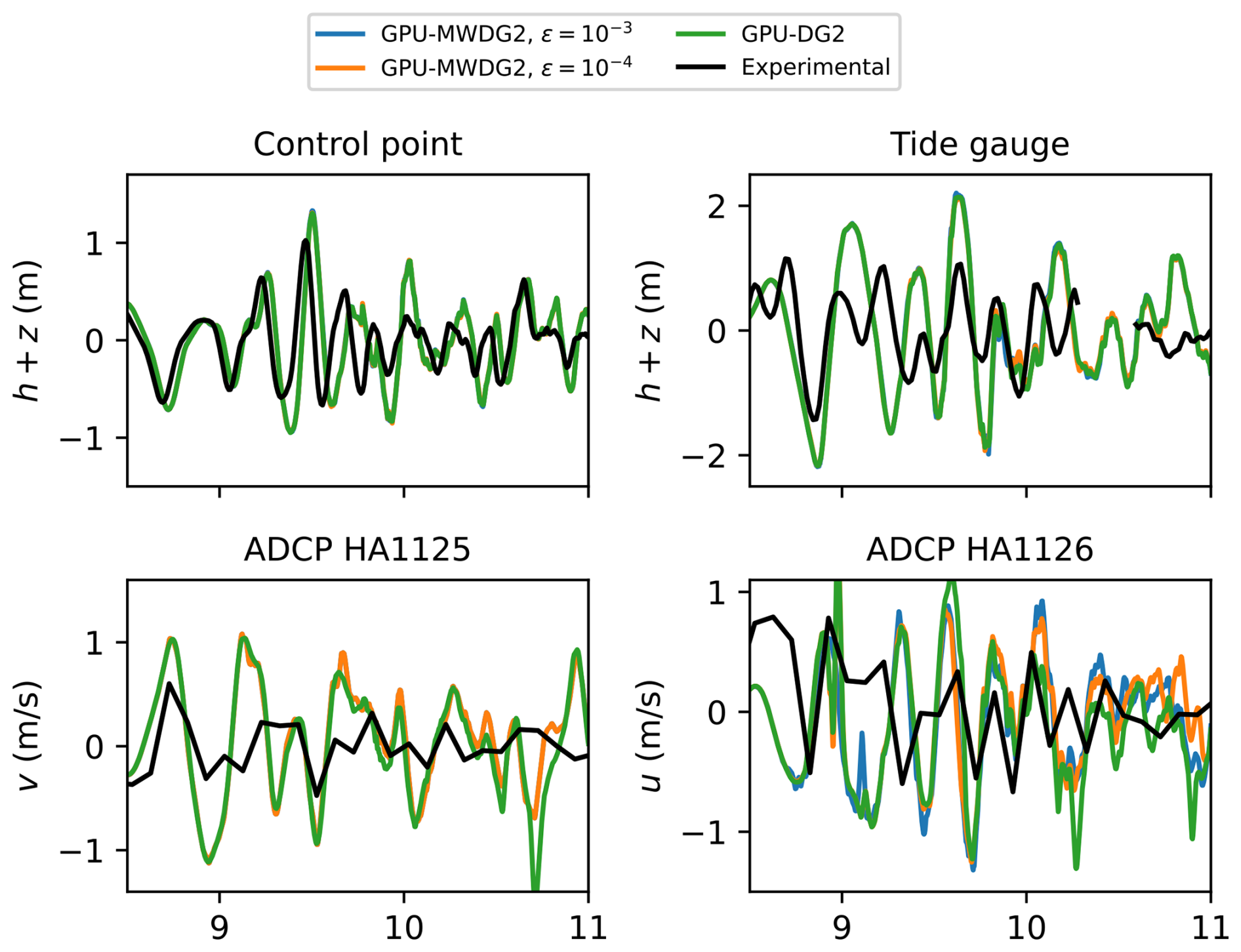
Figure 17Hilo Harbour. Time series produced by GPU-DG2 and GPU-MWDG2, for the water surface elevation (h+z) at “control point” and “Tide gauge” (labelled in the figure), and for the velocity components at “ADCP HA1125” and ADCP HA 1126 (labelled in the figure), compared to the experimental results.
Table 6Hilo Harbour. DE, FE and PE quantified using Eqs. (1) to (3) and considering measured vs predicted time series of the prognostic variable h+z at observation points Tide gauge and Control point, and of the prognostic variables v and u at observation points ADCP 1125 and 1126 respectively. The errors are considered in order to check for fulfilment of conditions (i) and (ii) and confirm the validity of selecting ε = 10−3 and 10−4 in this test case.
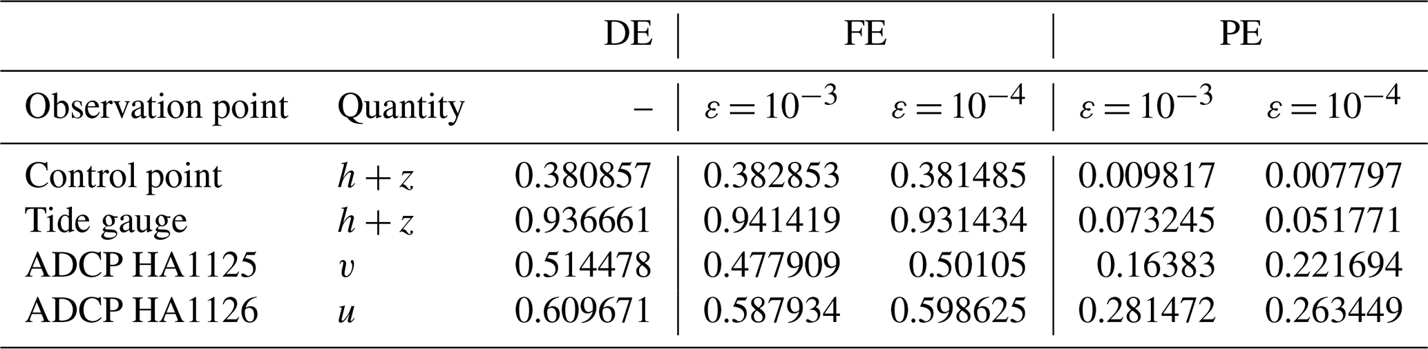
Table 6 shows the associated DE, FE and PE at the observation points. An outlier is noticeable in this test case for the FE at the Tide gauge and ADCP HA1125 observation points, which is actually smaller than the DE: this might be due missing data between 10 and 11 h (see the gap in the black line in the Tide gauge panel in Fig. 17). Nonetheless, generally, the DE and FE in the same order of magnitude, while the PE reduces when ε is decreased from 10−3 to 10−4, showing fulfilment of conditions (i) and (ii) and validating the choice of ε.
Table 7Summary of GPU-MWDG2 runtimes and potential average speedups with respect to GPU-DG2.
∗ By accounting for the physical scaling factor of the replica.
Overall, despite simulating a test case with a complex tsunami impact event and also a DEM size that requires selecting a small L = 10, GPU-MWDG2 still manages to attain speedups over GPU-DG2 in this test case: around 1.25 at ε = 10−3 and 1.10 at ε = 10−4. This seems to suggest that the GPU-MWDG2 solver can reliably be used to gain speedups over the GPU-DG2 solver even if simulating complex tsunami impact events, with both ε values being valid, using ε = 10−3 to boost the speedup, or using ε = 10−4 increase the quality of velocity predictions.
This work reported the new LISFLOOD-FP 8.2 hydrodynamic modelling framework, which integrates the GPU parallelised grid resolution adaptivity of multiwavelets (MW) within the second-order discontinuous Galerkin (DG2) solver of the shallow water equations (GPU-MWDG2) to run simulations on a non-uniform grid. The GPU-MWDG2 solver enables dynamic (in time) grid resolution adaptivity based on both the (time-varying) flow solution and the (time-invariant) Digital Elevation Model (DEM) representations. It is aimed at reducing the runtime of the existing uniform grid GPU parallelised DG2 solver (GPU-DG2) for flood simulation driven by rapid, multiscale impact events, which were exemplified by tsunami-induced flooding.
The usability of the LISFLOOD-FP 8.2 hydrodynamic modelling framework was presented focusing on: how to run GPU-MWDG2 simulations from raster-formatted DEM and initial flow condition setup files from a user-specified maximum refinement level L (i.e. ratio of the DEM size to its resolution) and an error threshold ε (i.e. recommended to be between 10−4 and 10−3); the effect of increasing L on GPU memory consumption and speedups; and, proposing new metrics for quantifying the speedups afforded by GPU-MWDG2 adaptivity against GPU-DG2 simulations.
The accuracy and efficiency of dynamic GPU-MWDG2 adaptivity was assessed for four laboratory- and field-scale tsunami-induced flood benchmarks featuring different impact event's complexity and duration (i.e. incorporating either single- or multi-peaked tsunamis and L = 10 or L = 12). GPU-MWDG2 simulation assessments were performed for ε = 10−3 and 10−4, which were also validated based on accuracy quantification with respect to benchmark-specific measured data. The accuracy assessment consistently confirms that an ε between 10−4 and 10−3 is valid: at ε = 10−3 GPU-MWDG2 simulations yield water level predictions as accurate as the GPU-DG2 predictions but using ε = 10−4 can slightly improve velocity-related predictions.
Speedup assessments, based on instantaneous and cumulative metrics, suggested considerable gain when the DEM size and resolution involved L ≥ 10 and for simulation durations that mostly spanned reduced-complexity events (i.e. single-peak tsunamis): As shown in Table 7, for single-peaked tsunamis, when the DEM required L = 10, GPU-MWDG2 was more than 2-fold faster than the GPU-DG2 simulations (i.e. “Monai Valley”), whereas with the DEM requiring L = 12, speedups of 3.3-to-4.5-fold could be achieved (i.e. “Seaside, Oregon”); in contrast, for multi-peaked tsunamis, GPU-MWDG2 speedups reduced to 1.8-fold for a DEM requiring L = 12 (i.e. “Tauranga Harbour”) and to 1.2-fold for a smaller DEM needing L = 10 (i.e. “Hilo Harbour”).
In summary, the GPU-MWDG2 solver in LISFLOOD-FP 8.2 consistently accelerates GPU-DG2 simulations of rapid multiscale flooding flows, generally yielding the greatest speedups for simulations needing L ≥ 10 – due to its scalability on the GPU which results in larger speedup with increasing L – and driven by single-peaked impact events. Choosing ε closer to 10−3 would maximise speedup while choosing an ε closer 10−4 may be useful to particularly improve the velocity-related predictions. The LISFLOOD-FP 8.2 code and the simulated benchmarks' set-up files and datasets are available under the code and data availability statement, while a video tutorial is available under the video supplement statement; further documentation is available at https://www.seamlesswave.com/Adaptive.
The GPU-MWDG2 algorithm that is integrated into LISFLOOD-FP 8.2 solves the two-dimensional shallow water equations over a non-uniform grid that locally adapts its grid resolution to the flow solutions and DEM representation every simulation timestep, Δt. The conservative form of the shallow water equations in vectorial format is as follows:
where ∂ represents a partial derivative operator; is the vector of the flow variables where T stands for the transpose operator, is the water depth (m) at time t and location (x,y), and and are the x- and y-component of the velocity field (m s−1) in two-dimensional Cartesian space; and are the components of the flux vector in which g is the gravitational acceleration constant (m s−2); is the bed-slope source term vector incorporating the partial derivative of the bed elevation function z(x,y); and is the friction source term vector including the friction effects as function of in which nM is Manning's roughness parameter. For ease of presentation, the scalar variable s will hereafter be used to represent any of the physical flow quantities in U as well as the bed elevation z.
Over each computational cell c, the DG2 modelled data for any of the any physical flow quantities, , follows a piecewise-planar solution, denoted by (Kesserwani and Sharifian, 2020). The piecewise-planar solution, , is expanded onto local basis functions from the scaled and truncated Legendre basis (Kesserwani et al., 2018; Kesserwani and Sharifian, 2020) to become spanned by three shape coefficients: , where is an average coefficient; and and are x- and y-directional slope coefficients, respectively (see Eq. 10 in Kesserwani and Sharifian, 2020). The bed elevation, s∈{z}, is also represented as piecewise-planar, but it is spanned by time-independent shape coefficients. The shape coefficients in sc, i.e. , must be initialised (Eq. 11 in Kesserwani and Sharifian, 2020), while only the time-dependent ones, i.e. , are updated using “DG2 solver updates” by an explicit two-stage Runge-Rutta scheme solving three ordinary differential equations:
where includes the respective components of the local discrete spatial DG2 operators to update each of the coefficients in . The operators in Lc were already designed to preserve mimetic properties by incorporating robust treatments of the bed and friction source terms and of moving wet-dry fronts (Kesserwani and Sharifian, 2020; Shaw et al., 2021).
The MWDG2 algorithm involves the MRA procedure to decompose, analyse and assemble the shape coefficients sc, into a non-uniform grid over which the DG2 solver updates are applied (Eq. A2). The MWDG2 algorithm was substantially redesigned to enable efficient parallelisation on the GPU (Chowdhury et al., 2023; Kesserwani and Sharifian, 2023): next, an overview of the GPU parallelised MWDG2 algorithm (GPU-MWDG2) is provided.
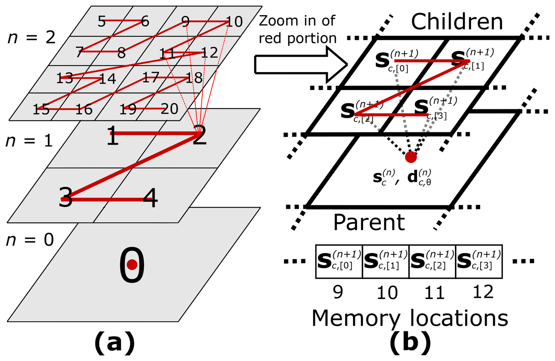
Figure A1Indexing and storage for the MRA procedure on the GPU. Panel (a) shows a hierarchy of grids across which cells are indexed along the Z-order curve. Panel (b) shows how four “children” cells at resolution level n+1, and their “parent” cell at resolution level n, noting that the shape coefficients at the “children” cells are stored in adjacent GPU memory locations.
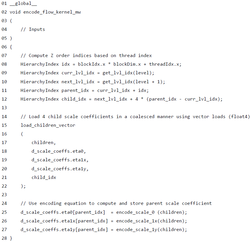
Algorithm A1Optimised CUDA kernel for performing the encoding operation in parallel. Coalesced memory access is ensured because the Z-order indices computed per thread point to adjacent memory locations in the array that is used to and . As seen in line 15, vectorised float4 loads can be used to load the children when computing the parent. Storing the parent is trivially coalesced due to the self-similar nature of Z-order indexing across refinement levels n and n+1.
In the CUDA programming model for parallelisation the GPU (NVIDIA Corporation, 2024), instructions are executed in parallel by workers called “threads”, and a group of 32 consecutive threads that operate in lockstep is called a “warp”. To devise an efficiently parallelised GPU-MWDG2 code, coalesced memory access, occurring when threads in a warp access contiguous memory locations, should be maximised, and warp divergence, occurring when threads within a single warp perform different instructions, should be minimised. To achieve these requirements in the GPU-MWDG2 code, the implementation of the MRA procedure had to be reformulated so as to ensure the DG2 solver updates are applicable cell-wise in a coalesced manner just like the GPU-parallelised DG2 solver (GPU-DG2) that runs on a uniform grid (Shaw et al., 2021).
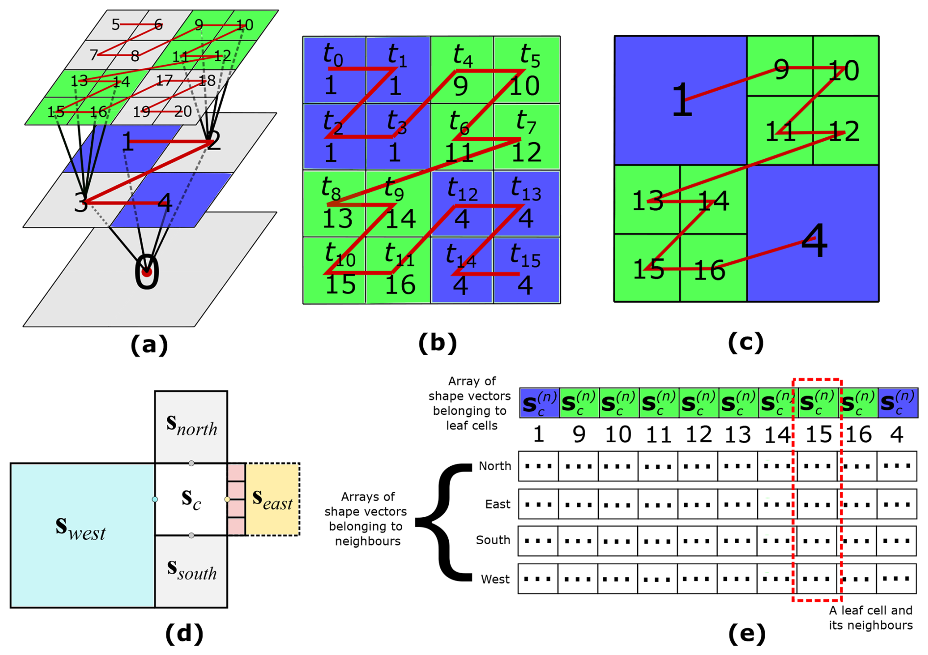
Figure A2Parallel tree traversal (PTT) and neighbour finding. (a) The tree-like structure obtained after flagging significant details during the process of encoding; (b) the leaf cells where the tree terminates (highlighted in green and blue); (c) leaf cells are assembly into the non-uniform grid; (d) possible scenarios of neighbouring cells to leaf cell c; and (e) leaf and neighbour cells storage as arrays in GPU memory.
A1 MRA procedure
The MRA procedure must start from a square uniform grid at the finest resolution, in particular at the given DEM resolution, which is defined to have a maximum refinement level, L. This finest grid contains 2L×2L cells, on which the shape coefficients are initialised. From the finest grid, the MRA procedure can be applied to build a hierarchy of grids of successively coarser resolution at levels , …, 1, 0, comprising 2n×2n cells each. Using the “encoding” operation, the shape coefficients, , and their associated “details”, , Θ=αβγ, can be produced on the “parent” cells of the coarser resolution grids, at level n, from the shape coefficients , , and of the four “children” cells at the finer resolution grids, at level n+1 (Eq. 30 in Kesserwani and Sharifian, 2020). With the GPU-MWDG2 solver, and are stored in arrays in GPU memory that are indexed using Z-order curves (Chowdhury et al., 2023), as exemplified in Fig. A1a for a simplistic case with L = 2. Hence, , , and all reside in adjacent memory locations when used to produce and (see Fig. A1b) and can be accessed using vectorised float4 instructions (see lines 7 to 22 of Algorithm A1) to ensure coalesced memory access. The produced can then be trivially stored in the appropriate index of the array (see lines 25 to 27 of Algorithm A1), again in a coalesced manner due to the self-similar nature of the Z-order curve between refinement levels n and n+1.
While encoding, the magnitude of all the details is analysed against ε in order to identify significant details (Kesserwani and Sharifian, 2020), which results in a tree-like structure of significant details (Fig. A2a). The MRA procedure then uses this tree to generate the non-uniform grid via the “decoding” operation. Decoding is applied within the hierarchy of grids, starting from the coarsest resolution grid until reaching a “leaf” cell where significant details reside (i.e. where a branch of the tree terminates, see Fig. A2a where leaf cells are coloured). After decoding, the shape vectors , , and at the leaf cells are stored on the non-uniform grid (Eq. 31 in Kesserwani and Sharifian, 2020) to be updated in time.
With the GPU-MWDG2 solver, decoding must be performed using a parallel tree traversal algorithm (PTT) to minimise warp divergence (Chowdhury et al., 2023). To do so, the PTT starts by launching as many threads tn as the number of cells on the finest resolution grid; for example, 16 threads t0 to t15 for traversing the tree in Fig. A2a. Each thread independently traverses the tree starting from the cell on the coarsest resolution grid until it reaches its leaf cell c, i.e. until it reaches either a detail that is no longer significant (line 14 of Algorithm A2) or the finest refinement level (line 28 of Algorithm A2). Once a thread reaches a leaf cell, it records the Z-order index of that leaf cell (Fig. A2b and c).
Algorithm A2Optimised CUDA kernel for performing parallel tree traversal (PTT) that minimises warp divergence. Threads keep traversing the tree of significant details until they reach either an insignificant detail or the finest refinement level. Warp divergence is reduced because threads that end up reaching nearby leaf cells have similar traversal paths.
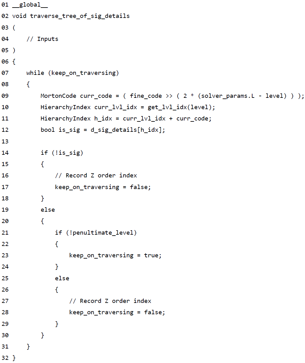
Figure A2b shows the indices of the leaf cells identified by each thread once PTT is complete. Since the PTT started with 16 threads and there are fewer leaf cells than the threads, many of threads ended up identifying the same index of the leaf cell (e.g., t0 to t3 identified the leaf cell with index 1 and t12 to t15 identified the leaf cell with index 4, all having finished execution at line 17 of Algorithm A2). Threads with duplicate indices are re-used, alongside the other threads, to search and record the indices of east, west, north, and south neighbouring cells of each leaf cell by making each thread look up, down, left, and right. For example, t0 to t3 of the leaf cell with index 1 will identify the east neighbour cells 9 and 11 (Fig. A2c). Since the DG2 solver updates on the leaf cell with index 1 requires the (shape coefficients of the) east neighbour cells (shaded red, Fig. A2d) to be at the same resolution level as the coarser leaf cell, the PPT will instead record the index of coarsened east neighbour cells (yellow shaded, Fig. A2d). For any other scenario (e.g., west, north, or south neighbour cells in Fig. A2d), the actual indices and shape coefficients are recorded by the PTT. After recording the indices and shape coefficients, , which are to unique each leaf cell c, and its neighbours, , , and , they are stored on the non-uniform grid (Fig. A2c). In particular, shape coefficients for the leaf cells, , are stored in a separate, contiguous arrays in GPU memory, and separate, contiguous arrays are also used to do the same for the shape coefficients of their neighbour cells, , , and (see Fig. A2e). With this cell-wise storage of indices and shape coefficients in contiguous arrays, the DG2 solver updates, Eq. (A2), can be applied in a coalesced manner.
A2 DG2 solver update on the non-uniform grid
On the non-uniform grid, the DG2 solver updates, Eq. (A2), are applied to update the shape coefficients by half a timestep over the first Runge-Kutta time stage. After this, another re-encoding step must be applied to the update shape coefficients so that the stored shape coefficients of the four neighbours, , , and , are also lifted by half a timestep. Now, the shape coefficients can be updated by a full timestep by completing the second of Runge-Kutta time stage.
This Appendix shows how to run a simulation of the “Monai valley” example (Sect. 3.1) using the GPU-MWDG2 solver step-by-step. To use the GPU-MWDG2 solver, the LISFLOOD-FP source code has to be downloaded (LISFLOOD-FP developers, 2024), and then an executable file that can be run has to be built, either on Windows or Linux. To build the executable file on Windows, (1) the LISFLOOD-FP folder should be opened in Visual Studio, (2) either the x64-Debug or x64-Release option should be selected from the dropdown menu near the toolbar at the top; and, (3) the Build > Rebuild All option should be clicked. If the x64-Debug option was selected, the executable file, named lisflood.exe and containing the GPU-MWDG2 solver, should be built and located in the folder at LISFLOOD-FP\out\build\x64-Debug or similar (or LISFLOOD-FP\out\build\x64-Release if the x64-Release option was selected). To build on Linux, the steps are (1) navigating to the LISFLOOD-FP directory, (2) running cmake -S . -B build in the terminal; and, (3) running cmake –build build. The executable file, named lisflood, should be built and located in the LISFLOOD-FP/build directory.
After the executable file has been built, it can be run in order to run simulations of the “Monai valley” example using the GPU-MWDG2 solver. Before running the simulation, several input files must be prepared, which are listed in Table B1. To prepare the input files, a number of Python scripts should be used that are available in the monai folder uploaded alongside the input files made publicly available online for reproducing the results and simulations reported in this paper (Chowdhury, 2024). The usage of these Python scripts is as follows.
Figure B1Input files displayed in File Explorer on Windows 10 as prepared for the “Monai valley” example after running the Python scripts available in the monai folder.
To prepare the input files for the Monai valley simulation using the Python scripts, (1) the monai folder should be copied to the same location as the lisflood.exe executable file, e.g. LISFLOOD-FP\out\build\x64-Release if on Windows or LISFLOOD-FP/build if on Linux, (2) the monai folder should be navigated to, (3) the monai.stage file should be generated by typing and running python stage.py in a command prompt, (4) the monai.dem and monai.start raster files should be generated by running python raster.py, (5) the monai.bci and monai.bdy files should be generated by running python inflow.py, (6) the parameter file monai.par should be prepared as shown in Fig. 2; and, (7) the simulation should be run by typing and running ..\lisflood.exe monai.par in a command prompt. Following steps (1) to (7) should result in the files shown in Fig. B1. Steps (1) to (7) can be performed as a fully automated process by running python run-simulations.py: this Python script will automatically prepare the input files (steps 3 to 6), run several simulations (step 7), and postprocess the results. Note that if run-simulations.py is run inside the downloaded monai folder before running any simulations, and with the self.run() function in the Python file commented out, it will reproduce the results in Sect. 3.1 (i.e. it will generate Figs. 7 and 8 and the data for Table 3).
Table B1Input files needed to run simulations of the Monai valley example using the GPU-MWDG2 solver.
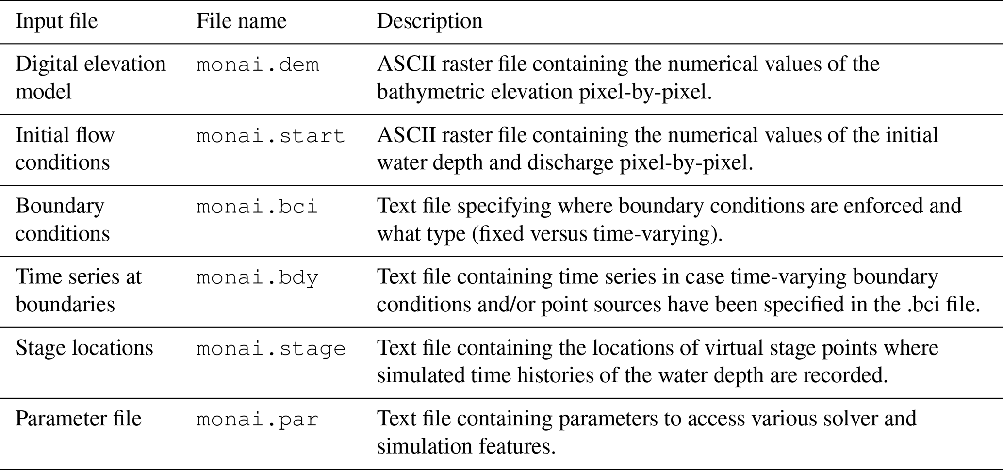
LISFLOOD-FP 8.2 source code is available from Zenodo (https://doi.org/10.5281/zenodo.13121102, LISFLOOD-FP developers, 2024) as well as the simulation results and input files/scripts for reproducing them (https://doi.org/10.5281/zenodo.13909072, Chowdhury, 2024); the GPU-MWDG2 solver code is also available at https://github.com/al0vya/gpu-mwdg2 (last access: 30 November 2025).
Step-by-step video tutorial on how to download, install and run the GPU-MWDG2 code for the “Monai Valley” example (Sect. 3.1) is available from Zenodo (https://doi.org/10.5281/zenodo.15851523, Chowdhury, 2025). The video demo also includes updates on the changes made to the CMake build process for compatibility with different versions of the CUDA toolkit.
AAC coded, optimised and integrated the GPU-MWDG2 into the LISFLOOD-FP framework (methodology; software; validation; investigation; data curation; visualization; formal analysis). GK contributed to the conceptualisation, formal analysis, funding acquisition and project administration. Both AAC and GK conceived and wrote the paper (original draft; review and editing).
The contact author has declared that neither of the authors has any competing interests.
Publisher's note: Copernicus Publications remains neutral with regard to jurisdictional claims made in the text, published maps, institutional affiliations, or any other geographical representation in this paper. While Copernicus Publications makes every effort to include appropriate place names, the final responsibility lies with the authors. Views expressed in the text are those of the authors and do not necessarily reflect the views of the publisher.
The authors are extremely grateful for Charles Rougé from the University of Sheffield for his feedback on the efficiency analysis of Sect. 3, and Paul Bates and Jefferey Neal from the University of Bristol for their support of the collaborative open source LISFLOOD-FP project.
For the purpose of open access, the authors have applied a Creative Commons Attribution (CC BY) licence to any Author Accepted Manuscript version arising.
AAC and GK were supported by the UK Engineering and Physical Sciences Research Council (EPSRC) (grant no. EP/R007349/1).
This paper was edited by Taesam Lee and reviewed by three anonymous referees.
Arcos, M. and LeVeque, R.: Validating Velocities in the GeoClaw Tsunami Model using Observations Near Hawaii from the 2011 Tohoku Tsunami, Pure Appl. Geophys., 172, https://doi.org/10.1007/s00024-014-0980-y, 2014.
Ayog, J. L., Kesserwani, G., and Baú, D.: Well-resolved velocity fields using discontinuous Galerkin shallow water, solutions, arXiv [physics.flu-dyn], https://doi.org/10.48550/arXiv.2104.11308, 2021.
Bates, P. D., Horritt, M. S., and Fewtrell, T. J.: A simple inertial formulation of the shallow water equations for efficient two-dimensional flood inundation modelling, J. Hydrol., 387, 33–45, https://doi.org/10.1016/j.jhydrol.2010.03.027, 2010.
Berger, M. J., George, D. L., LeVeque, R. J., and Mandli, K. T.: The GeoClaw software for depth-averaged flows with adaptive refinement, Adv. Water Resour., 34, 1195–1206, https://doi.org/10.1016/J.ADVWATRES.2011.02.016, 2011.
Blaise, S. and St-Cyr, A.: A Dynamic hp-Adaptive Discontinuous Galerkin Method for Shallow-Water Flows on the Sphere with Application to a Global Tsunami Simulation, Mon. Weather Rev., 140, 978–996, https://doi.org/10.1175/MWR-D-11-00038.1, 2012.
Blaise, S., St-Cyr, A., Mavriplis, D., and Lockwood, B.: Discontinuous Galerkin unsteady discrete adjoint method for real-time efficient tsunami simulations, J. Comput. Phys., 232, 416–430, https://doi.org/10.1016/j.jcp.2012.08.022, 2013.
Bonev, B., Hesthaven, J. S., Giraldo, F. X., and Kopera, M. A.: Discontinuous Galerkin scheme for the spherical shallow water equations with applications to tsunami modeling and prediction, J. Comput. Phys., 362, 425–448, https://doi.org/10.1016/j.jcp.2018.02.008, 2018.
Borrero, J. C., LeVeque, R. J., Greer, S. D., O'Neill, S., and Davis, B. N.: Observations and modelling of tsunami currents at the port of Tauranga, New Zealand, in: Australasian Coasts & Ports Conference 2015: 22nd Australasian Coastal and Ocean Engineering Conference and the 15th Australasian Port and Harbour Conference, ISBN 9781922107794, 2015.
Castro, C. E., Behrens, J., and Pelties, C.: Optimization of the ADER-DG method in GPU applied to linear hyperbolic PDEs, Int. J. Numer. Methods Fluids, 81, 195–219, https://doi.org/10.1002/fld.4179, 2016.
Caviedes-Voullième, D. and Kesserwani, G.: Benchmarking a multiresolution discontinuous Galerkin shallow water model: Implications for computational hydraulics, Adv. Water Resour., 86, 14–31, https://doi.org/10.1016/J.ADVWATRES.2015.09.016, 2015.
Caviedes-Voullième, D., Gerhard, N., Sikstel, A., and Müller, S.: Multiwavelet-based mesh adaptivity with Discontinuous Galerkin schemes: Exploring 2D shallow water problems, Adv. Water Resour., 138, 103559, https://doi.org/10.1016/J.ADVWATRES.2020.103559, 2020.
Chowdhury, A.: Dataset for the paper “LISFLOOD-FP 8.2: GPU-accelerated multiwavelet discontinuous Galerkin solver with dynamic resolution adaptivity for rapid, multiscale flood simulation” [data set], Zenodo, https://doi.org/10.5281/zenodo.13909072, 2024.
Chowdhury, A.: Simulation run guide for the GPU-MWDG2 solver in LISFLOOD-FP 8.2, Zenodo [video], https://doi.org/10.5281/zenodo.15851523, 2025.
Chowdhury, A. A., Kesserwani, G., Rougé, C., and Richmond, P.: GPU-parallelisation of Haar wavelet-based grid resolution adaptation for fast finite volume modelling: application to shallow water flows, Journal of Hydroinformatics, 25, 1210–1234, https://doi.org/10.2166/hydro.2023.154, 2023.
CUDA C++ Programming Guide: https://docs.nvidia.com/cuda/cuda-c-programming-guide/, last access: 23 March 2023.
de la Asunción, M. and Castro, M. J.: Simulation of tsunamis generated by landslides using adaptive mesh refinement on GPU, J. Comput. Phys., 345, 91–110, https://doi.org/10.1016/J.JCP.2017.05.016, 2017.
Ferreira, C. R. and Bader, M.: Load Balancing and Patch-Based Parallel Adaptive Mesh Refinement for Tsunami Simulation on Heterogeneous Platforms Using Xeon Phi Coprocessors, in: Proceedings of the Platform for Advanced Scientific Computing Conference, 12, https://doi.org/10.1145/3093172.3093237, 2017.
Gao, S., Collecutt, G., Syme, W. J., and Ryan, P.: High resolution numerical modelling of tsunami inundation using quadtree method and GPU acceleration, in: Proceedings of the 22nd IAHR-APD Congress (IAHR-APD 2020), ISBN 9781713827030, https://www.iahr.org/library/info?pid=7668 (last access: 30 November 2025), 2020.
Gerhard, N. and Müller, S.: Adaptive multiresolution discontinuous Galerkin schemes for conservation laws: multi-dimensional case, Computational and Applied Mathematics, 35, 321–349, https://doi.org/10.1007/s40314-014-0134-y, 2016.
Gerhard, N., Caviedes-Voullième, D., Müller, S., and Kesserwani, G.: Multiwavelet-based grid adaptation with discontinuous Galerkin schemes for shallow water equations, J. Comput. Phys., 301, 265–288, https://doi.org/10.1016/J.JCP.2015.08.030, 2015.
Hajihassanpour, M., Bonev, B., and Hesthaven, J. S.: A comparative study of earthquake source models in high-order accurate tsunami simulations, Ocean Model., 141, 101429, https://doi.org/10.1016/j.ocemod.2019.101429, 2019.
Hajihassanpour, M., Kesserwani, G., Pettersson, P., and Bellos, V.: Sampling-Based Methods for Uncertainty Propagation in Flood Modeling Under Multiple Uncertain Inputs: Finding Out the Most Efficient Choice, Water Resources Research, 59, e2022WR034011 https://doi.org/10.1029/2022WR034011, 2023.
Hunter, N. M., Horritt, M. S., Bates, P. D., Wilson, M. D., and Werner, M. G. F.: An adaptive time step solution for raster-based storage cell modelling of floodplain inundation, Adv. Water Resour., 28, 975–991, https://doi.org/10.1016/j.advwatres.2005.03.007, 2005.
Kesserwani, G.: Topography discretization techniques for Godunov-type shallow water numerical models: a comparative study, Journal of Hydraulic Research, 51, 351–367, https://doi.org/10.1080/00221686.2013.796574, 2013.
Kesserwani, G. and Liang, Q.: Dynamically adaptive grid based discontinuous Galerkin shallow water model, Adv. Water Resour., 37, 23–39, https://doi.org/10.1016/J.ADVWATRES.2011.11.006, 2012.
Kesserwani, G. and Liang, Q.: RKDG2 shallow-water solver on non-uniform grids with local time steps: Application to 1D and 2D hydrodynamics, Applied Mathematical Modelling, 39, 1317–1340, https://doi.org/10.1016/j.apm.2014.08.009, 2015.
Kesserwani, G. and Sharifian, M. K.: (Multi)wavelets increase both accuracy and efficiency of standard Godunov-type hydrodynamic models: Robust 2D approaches, Adv. Water Resour., 144, 103693, https://doi.org/10.1016/J.ADVWATRES.2020.103693, 2020.
Kesserwani, G. and Sharifian, M. K.: (Multi)wavelet-based Godunov-type simulators of flood inundation: Static versus dynamic adaptivity, Adv. Water Resour., 171, 104357, https://doi.org/10.1016/j.advwatres.2022.104357, 2023.
Kesserwani, G. and Wang, Y.: Discontinuous Galerkin flood model formulation: Luxury or necessity?, Water Resour. Res., 50, 6522–6541, https://doi.org/10.1002/2013WR014906, 2014.
Kesserwani, G., Caviedes-Voullième, D., Gerhard, N., and Müller, S.: Multiwavelet discontinuous Galerkin h-adaptive shallow water model, Comput. Methods Appl. Mech. Eng., 294, 56–71, https://doi.org/10.1016/j.cma.2015.05.016, 2015.
Kesserwani, G., Ayog, J. L., and Bau, D.: Discontinuous Galerkin formulation for 2D hydrodynamic modelling: Trade-offs between theoretical complexity and practical convenience, Comput. Methods Appl. Mech. Eng., 342, 710–741, https://doi.org/10.1016/J.CMA.2018.08.003, 2018.
Kesserwani, G., Shaw, J., Sharifian, M. K., Bau, D., Keylock, C. J., Bates, P. D., and Ryan, J. K.: (Multi)wavelets increase both accuracy and efficiency of standard Godunov-type hydrodynamic models, Adv. Water Resour., 129, 31–55, https://doi.org/10.1016/J.ADVWATRES.2019.04.019, 2019.
Kevlahan, N. K.-R. and Lemarié, F.: wavetrisk-2.1: an adaptive dynamical core for ocean modelling, Geosci. Model Dev., 15, 6521–6539, https://doi.org/10.5194/gmd-15-6521-2022, 2022.
Lee, H. S.: Tsunami run-up modeling with adaptive mesh refinement method: A case study for Monai Village run-up experiment, in: Proceedings of the 20th IAHR-APD Congress (Colombo, 2016), https://www.iahr.org/library/infor?pid=9478 (last access: 30 November 2025), 2016.
LeVeque, R. J., George, D. L., and Berger, M. J.: Tsunami modelling with adaptively refined finite volume methods, Acta Numerica, 20, 211–289, https://doi.org/10.1017/S0962492911000043, 2011.
Liang, Q., Hou, J., and Amouzgar, R.: Simulation of Tsunami Propagation Using Adaptive Cartesian Grids, Coastal Engineering Journal, 57, 1550016, https://doi.org/10.1142/S0578563415500163, 2015.
LISFLOOD-FP developers: LISFLOOD-FP v8.2 hydrodynamic model (8.2), Zenodo [code], https://doi.org/10.5281/zenodo.13121102, 2024.
Liu, P. L. F., Yeh, H., and Synolakis, C. E.: Advanced Numerical Models for Simulating Tsunami Waves and Runup, World Scientific, 344 pp., https://doi.org/10.1142/6226, 2008.
Lynett, P. J., Gately, K., Wilson, R., Montoya, L., Arcas, D., Aytore, B., Bai, Y., Bricker, J. D., Castro, M. J., Cheung, K. F., David, C. G., Dogan, G. G., Escalante, C., González-Vida, J. M., Grilli, S. T., Heitmann, T. W., Horrillo, J., Kânoğlu, U., Kian, R., Kirby, J. T., Li, W., Macías, J., Nicolsky, D. J., Ortega, S., Pampell-Manis, A., Park, Y. S., Roeber, V., Sharghivand, N., Shelby, M., Shi, F., Tehranirad, B., Tolkova, E., Thio, H. K., Velioğlu, D., Yalçıner, A. C., Yamazaki, Y., Zaytsev, A., and Zhang, Y. J.: Inter-model analysis of tsunami-induced coastal currents, Ocean Model., 114, 14–32, https://doi.org/10.1016/j.ocemod.2017.04.003, 2017.
Macías, J., Castro, M., Ortega, S., Escalante Sánchez, C., and González Vida, J.: Tsunami currents benchmarking results for Tsunami-HySEA, 115–135, https://doi.org/10.13140/RG.2.2.22999.47527, 2015.
Macías, J., Castro, M. J., and Escalante, C.: Performance assessment of the Tsunami-HySEA model for NTHMP tsunami currents benchmarking. Laboratory data, Coastal Engineering, 158, 103667, https://doi.org/10.1016/J.COASTALENG.2020.103667, 2020a.
Macías, J., Castro, M. J., Ortega, S., and González-Vida, J. M.: Performance assessment of Tsunami-HySEA model for NTHMP tsunami currents benchmarking. Field cases, Ocean Model., 152, 101645, https://doi.org/10.1016/j.ocemod.2020.101645, 2020b.
Matsuyama, M. and Tanaka, H.: An experimental study of the highest run-up height in the 1993 Hokkaido Nansei-Oki earthquake tsunami, in: Proceedings of the National Tsunami Hazard Mitigation Program Review and International Tsunami Symposium (ITS), 879–889, https://www.researchgate.net/publication/236646065_An_experimental_study_of_the_highest_run-up_height_in_the_1993_Hokkaido_Nansei-Oki_earthquake_tsunami (last access: 30 November 2025), 2001.
Nandi, S. and Reddy, M. J.: An integrated approach to streamflow estimation and flood inundation mapping using VIC, RAPID and LISFLOOD-FP, J. Hydrol., 610, 127842, https://doi.org/10.1016/j.jhydrol.2022.127842, 2022.
NVIDIA Corporation: CUDA C++ Programming Guidehttps://docs.nvidia.com/cuda/cuda-c-programming-guide/ (last access: 30 November 2025), 2024.
Park, H., Cox, D. T., Lynett, P. J., Wiebe, D. M., and Shin, S.: Tsunami inundation modeling in constructed environments: A physical and numerical comparison of free-surface elevation, velocity, and momentum flux, Coastal Engineering, 79, 9–21, https://doi.org/10.1016/j.coastaleng.2013.04.002, 2013.
Park, J., Yuk, J.-H., Joo, W., and Lee, H. S.: Wave Run-up Modeling with Adaptive Mesh Refinement (AMR) Method in the Busan Marine City during Typhoon Chaba (1618), J. Coast. Res., 91, 56, https://doi.org/10.2112/SI91-012.1, 2019.
Popinet, S.: Quadtree-adaptive tsunami modelling, Ocean Dyn., 61, 1261–1285, https://doi.org/10.1007/s10236-011-0438-z, 2011.
Popinet, S.: Adaptive modelling of long-distance wave propagation and fine-scale flooding during the Tohoku tsunami, Nat. Hazards Earth Syst. Sci., 12, 1213–1227, https://doi.org/10.5194/nhess-12-1213-2012, 2012.
Popinet, S. and Rickard, G.: A tree-based solver for adaptive ocean modelling, Ocean Model., 16, 224–249, https://doi.org/10.1016/j.ocemod.2006.10.002, 2007.
Qin, X., Motley, M., LeVeque, R., Gonzalez, F., and Mueller, K.: A comparison of a two-dimensional depth-averaged flow model and a three-dimensional RANS model for predicting tsunami inundation and fluid forces, Nat. Hazards Earth Syst. Sci., 18, 2489–2506, https://doi.org/10.5194/nhess-18-2489-2018, 2018.
Rannabauer, L., Dumbser, M., and Bader, M.: ADER-DG with a-posteriori finite-volume limiting to simulate tsunamis in a parallel adaptive mesh refinement framework, Comput. Fluids, 173, 299–306, https://doi.org/10.1016/j.compfluid.2018.01.031, 2018.
Sharifian, M. K., Kesserwani, G., and Hassanzadeh, Y.: A discontinuous Galerkin approach for conservative modeling of fully nonlinear and weakly dispersive wave transformations, Ocean Model., 125, 61–79, https://doi.org/10.1016/j.ocemod.2018.03.006, 2018.
Sharifian, M. K., Hassanzadeh, Y., Kesserwani, G., and Shaw, J.: Performance study of the multiwavelet discontinuous Galerkin approach for solving the Green-Naghdi equations, Int. J. Numer. Methods Fluids, 90, 501–521, https://doi.org/10.1002/fld.4732, 2019.
Sharifian, M. K., Kesserwani, G., Chowdhury, A. A., Neal, J., and Bates, P.: LISFLOOD-FP 8.1: new GPU-accelerated solvers for faster fluvial/pluvial flood simulations, Geosci. Model Dev., 16, 2391–2413, https://doi.org/10.5194/gmd-16-2391-2023, 2023.
Shaw, J., Kesserwani, G., Neal, J., Bates, P., and Sharifian, M. K.: LISFLOOD-FP 8.0: the new discontinuous Galerkin shallow-water solver for multi-core CPUs and GPUs, Geosci. Model Dev., 14, 3577–3602, https://doi.org/10.5194/gmd-14-3577-2021, 2021.
Sun, X., Kesserwani, G., Sharifian, M. K., and Stovin, V.: Simulation of laminar to transitional wakes past cylinders with a discontinuous Galerkin inviscid shallow water model, Journal of Hydraulic Research, 61, 631–650, https://doi.org/10.1080/00221686.2023.2239750, 2023.
Velioglu Sogut, D. and Yalciner, A. C.: Performance Comparison of NAMI DANCE and FLOW-3D® Models in Tsunami Propagation, Inundation and Currents using NTHMP Benchmark Problems, Pure Appl. Geophys., 176, 3115–3153, https://doi.org/10.1007/s00024-018-1907-9, 2019.
Violeau, D., Ata, R., Benoit, M., Joly, A., Abadie, S., Clous, L., Martin Medina, M., Morichon, D., Chicheportiche, J., Le Gal, M., Gailler, A., Hébert, H., Imbert, D., Kazolea, M., Ricchiuto, M., Le Roy, S., Pedreros, R., Rousseau, M., Pons, K., Marcer, R., Journeau, C., and Silva Jacinto, R.: A database of validation cases for tsunami numerical modelling, in: Proceedings of the 4th IAHR Europe Congress (IAHR Europe Congress, Liège), CRC Press, ISBN 9781138029774, https://www.iahr.org/library/infor?pid=10483 (last access: 30 November 2025), 2016.
Zeng, Z., Wang, Z., and Lai, C.: Simulation Performance Evaluation and Uncertainty Analysis on a Coupled Inundation Model Combining SWMM and WCA2D, International Journal of Disaster Risk Science, 13, 448–464, https://doi.org/10.1007/s13753-022-00416-3, 2022.
Ziliani, L., Surian, N., Botter, G., and Mao, L.: Assessment of the geomorphic effectiveness of controlled floods in a braided river using a reduced-complexity numerical model, Hydrol. Earth Syst. Sci., 24, 3229–3250, https://doi.org/10.5194/hess-24-3229-2020, 2020.
The CPU version of the MWDG2 solver was not integrated on LISFLOOD-FP due to its uncompetitive runtimes.
- Abstract
- Introduction
- LISFLOOD-FP 8.2
- Evaluation of GPU-MWDG2 adaptivity
- Conclusions and recommendations
- Appendix A: The GPU-MWDG2 algorithm
- Appendix B: Step-by-step instructions for running the “Monai valley” example
- Code and data availability
- Video supplement
- Author contributions
- Competing interests
- Disclaimer
- Acknowledgements
- Financial support
- Review statement
- References