Enhancing volcanic eruption simulations with the WRF-Chem v4.8

Volcanic eruptions are one of the major natural hazards, exerting profound effects on the environment and climate. The emissions associated with such eruptions pose substantial risks to terrestrial systems and public health, particularly through the induction of acid rain and air pollution. Volcanic ash influences populations at distances reaching several thousand kilometers from the erupted volcano. Also, accurate forecasting of volcanic clouds is crucial for air traffic control. This study introduces enhancements to the simulation of volcanic eruptions and the transport of volcanic material using the Weather Research and Forecasting model coupled with Chemistry (WRF-Chem) version 4.8. Improvements include the addition of wet and dry deposition of ash and sulfate, improved SO₂ chemical transformation mechanisms, and corrections of the gravitational deposition of ash. Ash, sulfate, and SO₂ mass balance analyses were conducted. Furthermore, we included the direct radiative effect of ash and sulfate aerosols. Additionally, we developed an open-source Python-written emission preprocessor called PrepEmisSources to facilitate and streamline the preparation of volcanic emissions. Accordingly, the model code was extended to simulate complex volcanic emission scenarios using the emissions file prepared using the PrepEmisSources tool. The results suggest that the enhanced WRF-Chem v4.8 code provides an accurate representation of volcanic ash, SO₂, and sulfate dispersion, deposition, and SO₂ chemical transformation. These improvements will aid in volcanic debris forecasting and will allow for the use of the model for assessments of volcanic aerosols on climate and for geoengineering problems, including modeling of stratospheric aerosol injection.

1 Introduction

Volcanic eruptions are one of the major natural hazards. The associated volcanic emissions pose substantial risks to agriculture, infrastructure, and public health, particularly through the tephra fallout, the induction of acid rain, and air pollution. Additionally, these emissions impact the climate by releasing sulfur dioxide (SO₂), which subsequently undergoes conversion into sulfate aerosols due to oxidation by hydroxyl radicals (OH) and hydrogen peroxide (H₂O₂). Volcanic aerosols influence extensive populations at distances reaching several thousand kilometers from the erupted volcano (Stewart et al., 2022). Moreover, information on ash concentration and the location of the volcanic ash cloud is essential for air traffic control (Casadevall, 1994). Considering these aspects, accurate numerical modeling of the transport and deposition of volcanic debris is essential.

Volcanic ash transport and dispersion models (VATDs) are widely used to forecast the dispersion and transport of ash clouds over hours to days to define hazards to aircraft and to communities downwind. These models are being used by nine Volcanic Ash Advisory Centers (VAACs) worldwide. VAACs provide forecasts on the expected presence of volcanic ash in the atmosphere to mitigate the risk to aviation. There are several VATD models; those include Euler and Lagrangian types of models, such as PUFF (Searcy et al., 1998), HYSPLIT (Stein et al., 2015), NAME (Jones et al., 2007), FLEXPART (Stohl et al., 2005), and FALL3D (Folch et al., 2009). These models are also useful in forecasting areas to be impacted by tephra fall. Most of the VATD models are “offline”, since they separately describe the physics and chemistry characterizing the dispersion of volcanic emissions in the atmosphere. Although “offline” models are fast, they do require the meteorological fields, which need to be computed in advance. These models do not fully capture interactions between meteorology and aerosol dynamics. Specifically, the interplay between volcanic aerosols and solar as well as terrestrial radiation exemplifies this form of interaction, which is not accounted for in the “offline” models. For example, important at the initial stage of the eruption ash particles have a relatively short lifetime. Erupted into the atmosphere, ash inhibits sunlight from reaching the Earth's surface, cooling the surface and warming the ash cloud due to strong absorption. In contrast, sulfate and sometimes water vapor are important in further stages of volcanic cloud dispersion. The stratospheric sulfate aerosol clouds can persist from a few months to a couple of years, reflecting solar radiation into space, inducing Earth's surface cooling (Stenchikov et al., 1998). The absorption of infrared upwelling radiation warms the layer where sulfate particles reside. In turn, being the most abundant greenhouse gas, water vapor plays a crucial role in global warming. Like CO₂ and CH₄, it absorbs and re-emits infrared radiation, trapping heat in the atmosphere and warming the planet. Therefore, a fully coupled “online” meteorology–chemistry model is a necessary tool to account for radiative feedback in simulating volcanic aerosols and meteorological fields.

1.1 Previous and related work

Among the available “online” tools, the coupled Weather Research and Forecasting model coupled with Chemistry (WRF-Chem) (Skamarock et al., 2005; Grell et al., 2005) open-source Eulerian model is distinguished for its capability to simulate atmospheric chemistry, air quality, transport, and deposition of aerosols, including volcanic ash. Webley et al. (2012), Stuefer et al. (2013), and Steensen et al. (2013) were the first who include in the WRF-Chem model the capability to simulate emissions from volcanoes and to predict the transport and concentration of ash and SO₂. In the model, ash is gravitationally settled, and SO₂ undergoes oxidation to sulfate using the prescribed OH vertical distribution. Stuefer et al. (2013) introduced ash size distribution classification and extended the volcanic emission preprocessor with time-variant emissions, which can either be specified directly as mass fluxes or calculated with the formula that relates plume height to the mass emission rate (Mastin et al., 2009). Webley et al. (2012) provided a detailed evaluation of the 2010 Eyjafjallajökull eruption in Iceland and successfully reproduced the observed plume structure. Steensen et al. (2013) conducted a qualitative comparison of the 2009 Mount Redoubt volcanic clouds using the PUFF and WRF-Chem models together with satellite observations, showing that WRF-Chem and PUFF produced comparable ash transport patterns. Hirtl et al. (2019) simulated the 2010 Eyjafjallajökull volcanic eruption to study ash dispersion and to highlight the importance of the radiative feedback effect on the meteorological fields. In particular, with enabled radiative feedback, a better agreement of volcanic cloud location with radiosonde measurements was achieved. Hirtl et al. (2020) made further extensions of the emission preprocessor introduced by Stuefer et al. (2013) to integrate complex sources. In particular, the volcanic preprocessor was integrated into the WRF-Chem code to allow the temporally and vertically resolved input data for the simulation of the eruption of the Grimsvötn volcano in Iceland in May 2011. Unfortunately, this code is not a part of the official release. Rizza et al. (2023) simulated a sequence of Mt. Etna paroxysms by coupling WRF-Chem with near-source L-band radar observations and demonstrated improved agreement between modeled and observed plume heights. Egan et al. (2020) analyzed tephra fallout and in situ airborne measurements of ash from the 2010 Eyjafjallajökull eruption, providing valuable validation data for volcanic ash dispersion modeling. de Bem et al. (2024) employed WRF-Chem to simulate ash transport from the 2015 Calbuco eruption in Chile and successfully reproduced the observed regional dispersion and deposition patterns. In Stenchikov et al. (2021), a modified version of the WRF-Chem model was used to evaluate the radiative effects of volcanic ash, sulfate, SO₂, and water vapor emitted during the Mt. Pinatubo eruption. They used the Goddard Chemistry Aerosol Radiation and Transport (GOCART) aerosol module (Chin et al., 2002) to represent ash as mineral dust with a modified complex refractive index (RI). The same approach was used in Ukhov et al. (2023) for inverse modeling of emission rates of ash and SO₂. Stenchikov et al. (2025) investigated the recent eruption of the Hunga Tonga–Hunga Haapai underwater volcano on 15 January 2022, which released 150 Mt of water vapor into the stratosphere. Water vapor strongly affected the dynamics of the aerosols as a result of the radiative cooling of the water vapor cloud.

Although the WRF-Chem model has been extensively utilized over the past decade and has demonstrated significant efficacy as a tool for forecasting the transport and dispersion of volcanic ash and SO₂ (Ukhov et al., 2020b, 2025), it still lacks a set of parameterizations. Furthermore, the interaction of ash and sulfate with solar and terrestrial radiation for the simulation of the direct radiative effect has not been implemented explicitly into the WRF-Chem code so far. There were only implicit attempts to account for only ash radiation interaction, ignoring the sulfate. In particular, Hirtl et al. (2019) redistributed the three finest ash bins into the PM_2.5 3D field, which was used in the calculation of the optical properties. This methodology presupposes a constant size distribution of PM_2.5, which constitutes a rather crude assumption considering the variability in the ash size distribution within the cloud, particularly in the initial days. In addition, the standard methodology for preparing volcanic emissions files using the open-source tool PREP-CHEM-SRC (Freitas et al., 2011) is notably cumbersome and not flexible.

1.2 Objectives of the current work

Here, we rectify the existing imperfections and add new capabilities to the WRF-Chem code v4.8 related to the simulation of volcanic eruptions. In particular, we account for major sinks: wet and dry deposition of ash, SO₂, sulfate, and SO₂ oxidation by OH and H₂O₂. We found and fixed an error in the subroutine for ash gravitational settling. Additionally, we establish a mass balance for SO₂, sulfate, and ash to ensure conservation of their mass. Moreover, we implemented the capability to simulate direct radiative effects of ash and sulfate aerosols, acknowledging the substantial radiative forcing exerted by volcanic eruptions on the climate system (Stenchikov et al., 2021). Recent studies (Stenchikov et al., 2025) highlight the importance of water vapor in modulating the dynamics of the volcanic plume. Therefore, simulation of emissions of water vapor and sulfate aerosol was also added. In addition, we developed an open-source emission preprocessor called PrepEmisSources (Ukhov and Hoteit, 2025). In contrast to the standard PREP-CHEM-SRC utility, our tool enhances the workflow and provides increased flexibility in defining the volcanic eruption process based on the eruption source parameters. More details are presented in Appendix A.

2 Code modifications

Most of the added code was adapted from the GOCART aerosol module (Chin et al., 2002) implemented in WRF-Chem. The GOCART module simulates major tropospheric aerosol components, including sulfate, dust, black and organic carbon, and sea salt, and includes algorithms for dust and sea salt emissions, dry deposition, and gravitational settling and oxidation of SO₂ (Ukhov et al., 2020a). We distinguish between gravitational settling and dry deposition processes. Gravitational settling refers to the downward motion of particles driven solely by gravity, affecting both ash and sulfate particles throughout the atmospheric column. In contrast, dry deposition is the surface removal process governed by aerodynamic resistance and surface characteristics (e.g., vegetation, roughness), acting primarily near the surface on particles and gases. Below, we describe the changes that we implemented in the WRF-Chem v4.8. Certain Sections incorporate pseudocode designed to compute some output diagnostics enumerated in Table B1. This inclusion is attributable to the absence of the necessary calculations for these diagnostics within the corresponding subroutines in the GOCART aerosol module.

2.1 SO₂ oxidation by OH and H₂O₂

We consider the chemical depletion of SO₂ resulting from oxidation processes. We replicate the code from the GOCART module, with modifications in the parameters used for the oxidation reaction with OH. The oxidation by H₂O₂, which had not been previously utilized in modeling volcanic SO₂, has been implemented within our study. See subroutine gocart_volc_chem_driver() in module_volc_chem.F for details. The oxidation is activated by setting gaschem_onoff = 1 in the namelist.input file. The OH and H₂O₂ fields are not computed interactively; instead, they are prescribed based on zonal and monthly mean OH and H₂O₂ fields (Liu et al., 2023) derived from the simulation of the Chemical Lagrangian Model of the Stratosphere (CLaMS) (Pommrich et al., 2014) and Copernicus Atmosphere Monitoring Service (CAMS) reanalysis (Inness et al., 2019), respectively. The “Code and data availability” section includes two Python scripts for interpolating OH and H₂O₂ fields into the WRF-Chem domain.

Three-body second-order reaction rate coefficient (k) of the SO₂-OH oxidation process: $\mathrm{OH}+{\mathrm{SO}}_{\mathrm{2}}+M\to \text{sulfates}+\mathrm{\dots }$ is calculated according to Table 2-1 in Burkholder et al. (2020) as follows:

$$\begin{array}{}\text{(1)}& k={\displaystyle \frac{k_{\mathrm{0}}\cdot M}{\mathrm{1}+\frac{k_{\mathrm{0}}\cdot M}{k_{\mathrm{\infty }}}}}\times {\mathrm{0.6}}^{\left(\mathrm{1}/\left(\mathrm{1}+{\log }_{\mathrm{10}}{\left(\frac{k_{\mathrm{0}}\cdot M}{k_{\mathrm{\infty }}}\right)}^{\mathrm{2}}\right)\right)}\left({\mathrm{cm}}^{\mathrm{3}}\mathrm{molec}{.}^{-\mathrm{1}}{\mathrm{s}}^{-\mathrm{1}}\right),\end{array}$$

where $k_{\mathrm{0}}=\mathrm{2.9}\times {\mathrm{10}}^{-\mathrm{31}}\times (\frac{\mathrm{298}}{T}{)}^{\mathrm{4.1}}$ (${\mathrm{cm}}^{\mathrm{6}}\mathrm{molec}{.}^{-\mathrm{2}}{\mathrm{s}}^{-\mathrm{1}}$) is the low-pressure limit rate,
$k_{\mathrm{\infty }}=\mathrm{1.7}\times {\mathrm{10}}^{-\mathrm{12}}\times (\frac{\mathrm{298}}{T}{)}^{-\mathrm{0.2}}$ (${\mathrm{cm}}^{\mathrm{3}}\mathrm{molec}{.}^{-\mathrm{1}}{\mathrm{s}}^{-\mathrm{1}}$) is the high-pressure limit rate,
T is the temperature (K), and M is the air density ($\mathrm{molec}.{\mathrm{cm}}^{-\mathrm{3}}$).

The updated SO₂ concentration (mol mol⁻¹) is calculated as follows:

$$\begin{array}{}\text{(2)}& {\mathrm{SO}}_{\mathrm{2}}={\mathrm{SO}}_{\mathrm{2}}\times \exp \left(-k\cdot \mathrm{OH}\cdot \mathrm{\Delta }t\right),\end{array}$$

where OH concentration is given in ($\mathrm{molec}.{\mathrm{cm}}^{-\mathrm{3}}$), and Δt is a time step (s). In general, the production of OH is driven by the photolysis of ozone, which causes a pronounced correlation with the diurnal cycle. To address this variability, the prescribed concentration of OH is multiplied by a scaling factor, which depends on the solar zenith angle.

In-cloud oxidation by hydrogen peroxide (H₂O₂) is another chemical sink for SO₂. Here we replicate the code implemented in the GOCART module. The loss of SO₂ due to aqueous-phase oxidation by H₂O₂ in clouds is parameterized following a simple cloud-fraction-weighted approach. The scheme applies only for grid cells where the temperature exceeds 258 K and the cloud fraction (f_c) is nonzero. To avoid excessive depletion when SO₂ exceeds the available H₂O₂, the effective cloud fraction $f_{\mathrm{c}}^{*}$ is scaled:

$$\begin{array}{}\text{(3)}& f_{\mathrm{c}}^{*}=\left\{\begin{array}{ll}{f}_{\mathrm{c}}\times \frac{{\mathrm{H}}_{\mathrm{2}}{\mathrm{O}}_{\mathrm{2}}}{{\mathrm{SO}}_{\mathrm{2}}},& \text{if }{\mathrm{SO}}_{\mathrm{2}}>{\mathrm{H}}_{\mathrm{2}}{\mathrm{O}}_{\mathrm{2}}\\ f_{\mathrm{c}},& \text{otherwise}\end{array}\right..\end{array}$$

SO₂ and H₂O₂ are given in (mol mol⁻¹). The post-reaction SO₂ is:

$$\begin{array}{}\text{(4)}& {\mathrm{SO}}_{\mathrm{2}}={\mathrm{SO}}_{\mathrm{2}}\times (\mathrm{1}-f_{\mathrm{c}}^{*}).\end{array}$$

This simple scheme ensures that aqueous SO₂ oxidation is limited by both cloud coverage and oxidant availability, without explicit kinetics of dissolution and reaction in cloud water.

2.2 Convective scavenging

The process of ash and sulfate scavenging through convective precipitation is incorporated within subroutine grelldrvct() implemented in module_ctrans_grell.F. This option is activated by setting conv_tr_wetscav = 1. The convective scavenging for SO₂ is not calculated, taking into account the assumption that all SO₂ undergoes oxidation within clouds. This process was not accounted for before in the simulation of ash and sulfate.

2.3 Large-scale scavenging

Here, large-scale scavenging represents in-cloud removal processes associated with stratiform clouds, as opposed to convective precipitation. The code for large-scale scavenging of ash, sulfate, and SO₂ is based on the one used for GOCART aerosols and gases. We implemented the code in the subroutine wetdep_ls_volc() in the module_vash_settling.F file. This option is activated by setting wetscav_onoff to any negative number. The scavenging process is applied to ash, SO₂, and sulfate. This scheme has a tuning parameter α, which is the scavenging efficiency. We set α=0.5 for ash and α=1 for SO₂ and sulfate, due to their high solubility and efficient removal in cloud water. We added the corresponding diagnostics, which reflect the accumulated amount of scavenged ash, SO₂, and sulfate:

$$\begin{array}{}\text{(5)}& {\displaystyle }\begin{array}{rl}& \text{WD\_ASH\_SC}=\\ & \mathrm{\text{WD\_ASH\_SC}}+\sum _{i=\mathrm{1}}^{\mathrm{10}}\left[\text{dvash\_}i\right]\cdot \mathit{\rho }\cdot \mathrm{\Delta }z\cdot {\mathrm{10}}^{-\mathrm{6}}\left(\mathrm{g}{\mathrm{m}}^{-\mathrm{2}}\right),\end{array}\text{(6)}& {\displaystyle }\begin{array}{rl}& \text{WD\_SO2\_SC}=\\ & \text{WD\_SO2\_SC}+\left[\mathrm{d}{\mathrm{SO}}_{\mathrm{2}}\right]\cdot \mathit{\rho }\cdot \mathrm{\Delta }z/\mathrm{28.97}\left(\mathrm{mmol}{\mathrm{m}}^{-\mathrm{2}}\right),\end{array}\text{(7)}& {\displaystyle }\begin{array}{rl}& \text{WD\_SULF\_SC}=\\ & \mathrm{\text{WD\_SULF\_SC}}+\left[\text{dsulf}\right]\cdot \mathit{\rho }\cdot \mathrm{\Delta }z/\mathrm{28.97}\left(\mathrm{mmol}{\mathrm{m}}^{-\mathrm{2}}\right).\end{array}\end{array}$$

These formulas are applied for each layer of the atmospheric column, where Δz is the layer width, [dSO₂], [dsulf], [dvash_i] are the computed fractions of concentrations of SO₂ (ppmv), sulfate (ppmv), and ash (µg kg⁻¹) in the ith bin, respectively, subjected to scavenging within the timestep at a specific layer of the atmospheric column. ρ is the dry air density (kg m⁻³), 28.97 (g mol⁻¹) is the air molar mass. These diagnostic formulas were previously absent in the GOCART module; nonetheless, they can be integrated by adhering to our proposed methodology.

2.4 Dry deposition

Dry deposition of SO₂, sulfate, and ash was implemented by analogy with the GOCART module, where dry deposition is combined with vertical mixing and activated by setting vertmix_onoff = 1. We implemented the code in the module_vash_settling.F file in the volc_ash_sulf_so2_drydep_driver() subroutine. Dry deposition velocity is calculated according to Wesely (2007) and used as a boundary condition near the surface for the flux of the species. The dry deposition removes aerosols from the lowermost model layer as a dry deposition flux. The accumulated amounts of SO₂, sulfate, and ash are computed using the following expressions:

$$\begin{array}{}\text{(8)}& {\displaystyle }\begin{array}{rl}& \text{SO2\_DRYDEP}=\\ & \text{SO2\_DRYDEP}\\ & +\left[{\mathrm{SO}}_{\mathrm{2}}\right]\cdot V_{\text{dry,}{\mathrm{SO}}_{\mathrm{2}}}\cdot \mathit{\rho }\cdot \mathrm{\Delta }t\cdot {\mathrm{10}}^{-\mathrm{6}}/\mathrm{28.97}\left(\mathrm{mol}{\mathrm{m}}^{-\mathrm{2}}\right),\end{array}\text{(9)}& {\displaystyle }\begin{array}{rl}& \text{SULF\_DRYDEP}=\\ & \text{SULF\_DRYDEP}\\ & +\left[\text{sulf}\right]\cdot V_{\text{dry,sulf}}\cdot \mathit{\rho }\cdot \mathrm{\Delta }t\cdot {\mathrm{10}}^{-\mathrm{6}}/\mathrm{28.97}\left(\mathrm{mol}{\mathrm{m}}^{-\mathrm{2}}\right),\end{array}\text{(10)}& {\displaystyle }\begin{array}{rl}& \text{ASH\_DRYDEP}=\\ & \text{ASH\_DRYDEP}\\ & +\left(\sum _{i=\mathrm{1}}^{\mathrm{10}}\left[\text{vash\_}i\right]\cdot V_{\text{dry,vash\_}i}\right)\cdot \mathit{\rho }\cdot \mathrm{\Delta }t\cdot {\mathrm{10}}^{-\mathrm{9}}\left(\mathrm{kg}{\mathrm{m}}^{-\mathrm{2}}\right).\end{array}\end{array}$$

[SO₂], [sulf], [vash_i] are the corresponding concentrations of SO₂ (ppmv), sulfate (ppmv), and ash (µg kg⁻¹) in the ith bin, Δt is the timestep (s), and $V_{\text{dry,}{\mathrm{SO}}_{\mathrm{2}}}$, V_dry,Sulf, and V_{dry,vash_i} are the computed dry deposition velocities (m s⁻¹) for ash particles in ith bin.

2.5 Gravitational settling of sulfate aerosols

As in the GOCART aerosol module, a bulk (single moment) approach is used to represent sulfate aerosols. In this approach, only the mass mixing ratio is tracked, and the assumed size distribution is fixed. Based on observations Borrmann et al. (1995) and Dessler et al. (2014), we assume that the volcanic sulfate aerosol number-density size distribution can be approximated by Aitken and accumulation lognormal modes. Aitken mode has a median radius r₁=0.09 µm and the geometric width σ₁=1.4. The accumulation mode has a median radius r₂=0.32 µm and the geometric width σ₂=1.6. Volcanic sulfate aerosol droplets in the troposphere have diameters smaller than 0.2 µm. Therefore, in the troposphere, only dry and wet scavenging of sulfate aerosols is usually considered. In contrast, in the stratosphere, the volcanic sulfate aerosol droplets are bigger, air density is lower, and gravitational settling becomes the leading deposition process. Therefore, we implemented the gravitational settling of sulfate aerosols following the same assumptions as in Stenchikov et al. (2021). Sulfate gravitational settling numerical scheme is implemented and adapted from the dust gravitational deposition scheme used in the GOCART scheme (Ukhov et al., 2021). Sulfate aerosol density is 1800 kg m⁻³. Only sulfate particles in the accumulation mode are gravitationally settled, assuming their wet mean radius of volume size distribution. Firstly, we determine dry radii R_dry,sulf calculated for sulfate aerosol volume median radii:

$$\begin{array}{}\text{(11)}& R_{\text{dry,sulf}}=r_{\mathrm{2}}\cdot \exp (\mathrm{3}\cdot \log ({\mathit{\sigma }}_{\mathrm{2}}{)}^{\mathrm{2}}).\end{array}$$

We obtain that R_dry,sulf=0.62 µm at given parameters of the accumulation lognormal mode. Secondly, sulfate aerosol wet radius (R_wet,sulf) is defined by computed R_dry,sulf, relative humidity RH, and hygroscopic parameter κ:

$$\begin{array}{}\text{(12)}& R_{\text{wet,sulf}}=R_{\text{dry,sulf}}\cdot {\left({\displaystyle \frac{\mathrm{1}+\text{RH}\cdot (\mathit{\kappa }-\mathrm{1})}{\mathrm{1}-\text{RH}}}\right)}^{\frac{\mathrm{1}}{\mathrm{3}}}.\end{array}$$

Following Aquila et al. (2012), we assume a hygroscopicity parameter of κ=1.19 for sulfate particles, which contrasts with κ=0.5 used in the calculation of sulfate optical properties (see Sect. 2.8). We found that κ=0.5 produced unrealistically small R_wet,sulf values, resulting in slower gravitational settling and artificial accumulation of sulfate in the troposphere. In contrast, using κ=1.19 increased R_wet,sulf, and, consequently, the gravitational deposition velocity, yields a more realistic vertical distribution and removal rate of sulfate aerosols. Furthermore, we verified that κ=1.19 results in an H₂SO₄–H₂O binary solution weight fraction in the range of 60 %–90 %, consistent with observational estimates for stratospheric sulfate aerosols.

The sulfate gravitational settling is implemented in module_vash_settling.F subroutine sulf_settling_driver(). The accumulated amount of gravitationally settled sulfate is computed as follows:

$$\begin{array}{}\text{(13)}& \begin{array}{rl}& \text{SULF\_GRAV\_SETL}=\\ & \text{SULF\_GRAV\_SETL}\\ & +\left[\text{SULF}\right]\cdot V_{\text{settling,Sulf}}\cdot \mathit{\rho }\cdot \mathrm{\Delta }t\cdot {\mathrm{10}}^{-\mathrm{9}}\left(\mathrm{kg}{\mathrm{m}}^{-\mathrm{2}}\right),\end{array}\end{array}$$

where [SULF] sulfate concentration (µg kg⁻¹), and V_{settling,Sulf} is the computed settling velocity (m s⁻¹) of sulfate particles.

2.6 PM calculations

For convenience, we also added diagnostic output containing computed PM_2.5 and PM₁₀ surface concentrations. We modified PM₁₀ and PM_2.5 calculations by analogy with Ukhov et al. (2021). The subroutine sum_pm_gocart() in module_volc_chem.F calculates PM_2.5 and PM₁₀ surface concentrations using the following formulas:

$$\begin{array}{}\text{(14)}& {\displaystyle }{\mathrm{PM}}_{\mathrm{2.5}}=\mathit{\rho }\cdot (\mathrm{1.375}\cdot \text{sulf}+\mathrm{0.672}\cdot \text{vash\_}\mathrm{10}),\text{(15)}& {\displaystyle }\begin{array}{rl}{\mathrm{PM}}_{\mathrm{10}}=\mathit{\rho }\cdot (& \mathrm{1.375}\cdot \text{sulf}+\text{vash\_}\mathrm{10}+\text{vash\_}\mathrm{9}\\ & +\mathrm{0.356}\cdot \text{vash\_}\mathrm{8}),\end{array}\end{array}$$

Factor 1.375 compensates for missing NH₄, which neutralizes sulfate and produces ammonium sulfate. sulf is sulfate concentration converted from ppmv to µg kg⁻¹, ρ is the dry air density (kg m⁻³), $\text{vash\_}\mathrm{8},\mathrm{9},\mathrm{10}$ are the mixing ratios (µg kg⁻¹) of the ash in the smallest three bins. Coefficients 0.672 and 0.356 are computed assuming that ash volume size distributions are functions of the natural logarithm of the particle radius, see Ukhov et al. (2021) for details.

2.7 Ash gravitational settling

The gravitational settling of aerosols is a key driver of their removal from the atmosphere. The modeled volcanic ash is subdivided into different bins representing the size spectrum of the particles. In WRF-Chem, ash particles are categorized into 10 size bins based on their radii, ranging from 0.01955 to 1000.0 µm, see Table 1. Ash can be modeled using 4 or 10 ash bins (chem_opt =403 or chem_opt $=\mathrm{400},\mathrm{402}$, respectively). For the ash gravitational settling, the terminal velocities are calculated for the mean arithmetic radii (R_m) within each bin size. Ash density is assumed to be 2500 kg m⁻³, see Table 1.

Table 1 Ash particle bin size ranges with corresponding WRF-Chem ash bins.

2.7.1 Correction of terminal velocity for large ash particles

For particles with a diameter D<10 µm, the Stokes law (Stokes, 1850), along with the Cunningham slip correction factor C_c (Cunningham, 1910), accurately describes the settling speed of particles. For such particles, the slip correction term dominates. However, the settling speed of larger particles deviates substantially from Stokes' law. In WRF-Chem, particles' radii span over several orders of magnitude. However, the required large particle drag correction is not accounted for in the code, which leads to a strong overestimation of the settling velocities.

Therefore, based on the approach proposed in Mailler et al. (2023), we corrected the settling velocity for vash_1..6 bins covering the mean arithmetic radii range from 500 to 23.44 µm. Their derivation is based on the Clift and Gauvin (1971) drag coefficient formulation and provides an approximated expression of the large-particle drag correction factor. The C_c is estimated based on the Davies (1945) expression as follows:

$$\begin{array}{}\text{(16)}& C_{\mathrm{c}}=\mathrm{1}+\mathit{\text{Kn}}\left(\mathrm{1.257}+\mathrm{0.4}\exp \left({\displaystyle \frac{-\mathrm{1.1}}{\mathit{\text{Kn}}}}\right)\right),\end{array}$$

where Kn is the Knudsen number of the particle with diameter D:

$$\begin{array}{}\text{(17)}& \mathit{\text{Kn}}={\displaystyle \frac{\mathrm{2}\mathit{\lambda }}{D}},\end{array}$$

where λ is the mean free path of molecules in air.

Stokes terminal velocity, including the slip correction term, is computed as follows:

$$\begin{array}{}\text{(18)}& {\stackrel{\mathrm{̃}}{v}}_{\mathrm{\infty }}^{\text{Stokes}}=C_{\mathrm{c}}{\displaystyle \frac{D^{\mathrm{2}}({\mathit{\rho }}_{\mathrm{p}}-{\mathit{\rho }}_{\mathrm{a}})g}{\mathrm{18}\mathit{\mu }}},\end{array}$$

where ρ_p and ρ_a are the particles' and air densities, respectively, and g is the gravitational acceleration constant.

The following equation takes into account both the slip correction factor and the large-particle drag correction factor:

$$\begin{array}{}\text{(19)}& v_{\mathrm{\infty }}={\stackrel{\mathrm{̃}}{v}}_{\mathrm{\infty }}^{\text{Stokes}}\times \left[\mathrm{1}-{\left(\mathrm{1}+{\left({\displaystyle \frac{\stackrel{\mathrm{̃}}{R}}{\mathrm{2.440}}}\right)}^{-\mathrm{0.4335}}\right)}^{-\mathrm{1.905}}\right],\end{array}$$

where parameter $\stackrel{\mathrm{̃}}{R}$ is defined as follows:

$$\begin{array}{}\text{(20)}& \stackrel{\mathrm{̃}}{R}={\displaystyle \frac{{\mathit{\rho }}_{\mathrm{a}}D{\stackrel{\mathrm{̃}}{v}}_{\mathrm{\infty }}^{\text{Stokes}}}{\mathrm{2}\mathit{\mu }}},\end{array}$$

For $\stackrel{\mathrm{̃}}{R}<\mathrm{0.0116}$, Eq. (19) can be replaced as follows:

$$\begin{array}{}\text{(21)}& v_{\mathrm{\infty }}={\stackrel{\mathrm{̃}}{v}}_{\mathrm{\infty }}^{\text{Stokes}}.\end{array}$$

The accumulated amount of ash deposited by gravitational settling across all bins is determined as follows:

$$\begin{array}{}\text{(22)}& {\displaystyle }\begin{array}{rl}& \text{ASH\_FALL}=\\ & \text{ASH\_FALL}\\ & +\left(\sum _{i=\mathrm{1}}^{\mathrm{10}}\left[\text{vash\_}i\right]\cdot V_{\mathrm{\infty },\text{vash\_}i}\right)\cdot \mathit{\rho }\cdot \mathrm{\Delta }t\cdot {\mathrm{10}}^{-\mathrm{9}}\left(\mathrm{kg}{\mathrm{m}}^{-\mathrm{2}}\right),\end{array}\end{array}$$

where [vash_i] is the concentration of ash (µg kg⁻¹) in the ith bin, and V_{∞,vash_i} are the computed settling velocities (m s⁻¹) for ash particles in ith bin.

2.7.2 Corrections in ash settling

We found that in the WRF-Chem code, the gravitational settling of volcanic ash was calculated incorrectly. The finite-difference scheme (implemented in the subroutine vsettling() file module_vash_settling.F) does not account for the change in air density when the deposition mass flux is being calculated. Ash is usually emitted into high altitudes, where air density is less than on the surface. Thus, in the course of the gravitational settling, the total ash in the atmosphere increases, violating the mass balances. We rectified this issue using a modified version of the finite-difference scheme, which conserves the mass of ash in the atmosphere. Below, we describe the implemented changes.

The change of aerosol mass due to gravitational settling at downward directed settling velocity w (m s⁻¹) is described using the conservative (flux) form for the integration of prognostic equations (Grell et al., 2005):

$$\begin{array}{}\text{(23)}& {\displaystyle \frac{\partial \left(qm\right)}{\partial t}}={\displaystyle \frac{\partial \left(qmw\right)}{\partial z}},\end{array}$$

where q is a ash mixing ratio (µg kg⁻¹), and m is the dry air mass (kg). This equation can be discretized into the following form:

$$\begin{array}{}\text{(24)}& \begin{array}{rl}& {\displaystyle \frac{q_k^{n+\mathrm{1}}{m}_k^{n+\mathrm{1}}-q_k^n{m}_k^n}{\mathrm{\Delta }t}}=\\ & {\displaystyle \frac{q_{k+\mathrm{1}}^{n+\mathrm{1}}{m}_{k+\mathrm{1}}^{n+\mathrm{1}}{w}_{k+\mathrm{1}}^{n+\mathrm{1}}-q_k^{n+\mathrm{1}}{m}_k^{n+\mathrm{1}}{w}_k^{n+\mathrm{1}}}{\mathrm{\Delta }{z}_k}},\end{array}\end{array}$$

where Δz_k is the height of the k model level, Δt is the model time step. Subscript k denotes the model levels and superscript n is the time-level. Taking into account that the calculation of gravitational settling is split from the calculation of the continuity equation, we assume $m_k^{n+\mathrm{1}}\approx m_k^n$ and get the following:

$$\begin{array}{}\text{(25)}& \begin{array}{rl}{q}_k^{n+\mathrm{1}}& -{\displaystyle \frac{\mathrm{\Delta }t}{\mathrm{\Delta }{z}_{k+\mathrm{1}}}}{q}_{k+\mathrm{1}}^{n+\mathrm{1}}{\displaystyle \frac{m_{k+\mathrm{1}}^{n+\mathrm{1}}}{m_k^n}}{w}_{k+\mathrm{1}}^{n+\mathrm{1}}\\ & +{\displaystyle \frac{\mathrm{\Delta }t}{\mathrm{\Delta }{z}_k}}{q}_k^{n+\mathrm{1}}{w}_k^{n+\mathrm{1}}=q_k^n.\end{array}\end{array}$$

Rewriting Eq. (25) taking into account that $m_k^n={\mathit{\rho }}_k^n\mathrm{\Delta }{z}_k\mathrm{\Delta }x\mathrm{\Delta }y$ and $m_{k+\mathrm{1}}^{n+\mathrm{1}}={\mathit{\rho }}_{k+\mathrm{1}}^{n+\mathrm{1}}\mathrm{\Delta }{z}_{k+\mathrm{1}}\mathrm{\Delta }x\mathrm{\Delta }y$ (where ρ and Δx Δy are the dry air density (kg m⁻³) and cell area (m²), respectively) gives the following:

$$\begin{array}{}\text{(26)}& \begin{array}{rl}& q_k^{n+\mathrm{1}}\left(\mathrm{1}+{\displaystyle \frac{\mathrm{\Delta }t{w}_k^{n+\mathrm{1}}}{\mathrm{\Delta }{z}_k}}\right)\\ & -{\displaystyle \frac{\mathrm{\Delta }t{w}_{k+\mathrm{1}}^{n+\mathrm{1}}}{\mathrm{\Delta }{z}_{k+\mathrm{1}}}}{q}_{k+\mathrm{1}}^{n+\mathrm{1}}\left({\displaystyle \frac{{\mathit{\rho }}_{k+\mathrm{1}}^{n+\mathrm{1}}\mathrm{\Delta }{z}_{k+\mathrm{1}}\mathrm{\Delta }x\mathrm{\Delta }y}{{\mathit{\rho }}_k^n\mathrm{\Delta }{z}_k\mathrm{\Delta }x\mathrm{\Delta }y}}\right)=q_k^n.\end{array}\end{array}$$

Rearranging Eq. (26) gives the following solution for $q_k^{n+\mathrm{1}}$:

$$\begin{array}{}\text{(27)}& q_k^{n+\mathrm{1}}=\left(q_k^n+{\displaystyle \frac{\mathrm{\Delta }t{w}_{k+\mathrm{1}}}{\mathrm{\Delta }{z}_k}}{q}_{k+\mathrm{1}}^{n+\mathrm{1}}{\displaystyle \frac{{\mathit{\rho }}_{k+\mathrm{1}}}{{\mathit{\rho }}_k}}\right){\left(\mathrm{1}+{\displaystyle \frac{\mathrm{\Delta }t{w}_k}{\mathrm{\Delta }{z}_k}}\right)}^{-\mathrm{1}}.\end{array}$$

Equation (27) is solved for each model column from the top to the bottom. For the topmost layer Eq. (27) transforms into:

$$\begin{array}{}\text{(28)}& q_k^{n+\mathrm{1}}=q_k^n{\left(\mathrm{1}+{\displaystyle \frac{\mathrm{\Delta }t{w}_k}{\mathrm{\Delta }{z}_k}}\right)}^{-\mathrm{1}}.\end{array}$$

Previous implementation of the finite difference scheme in the ash settling routine did not account for the dry air density ratio in Eq. (27). Consequently, when ash particles are settling from higher altitudes, a larger error is accumulated.

2.8 Inclusion of ash and sulfate into radiation calculation

The treatment of optically active ash and sulfate is vitally important. In particular, absorbing solar radiation, ash heats the atmosphere and is lofted (Stenchikov et al., 2021; Abdelkader et al., 2022). Ash has a relatively short lifetime and does not affect the climate much. While sulfate aerosols scatter solar radiation, have a longer lifetime, and play a primary role in aerosol–climate interactions.

By analogy with the subroutine optical_prep_gocart() being called for the calculation of volume-averaged refractive index (RI) when the GOCART aerosol module is being used, we implemented the subroutine optical_prep_volc() in module_optical_averaging.F file. This subroutine computes the volume-averaged RI needed for Mie calculations. The RI of $\text{ash}=\mathrm{1.550}+i\mathrm{0.001}$ in the shortwave spectral range has been chosen to approximate ash optical properties (Pollack et al., 1973; Carn and Krotkov, 2016). The larger imaginary part of the RI corresponds to the stronger absorption of solar radiation, enhancing atmospheric heating.

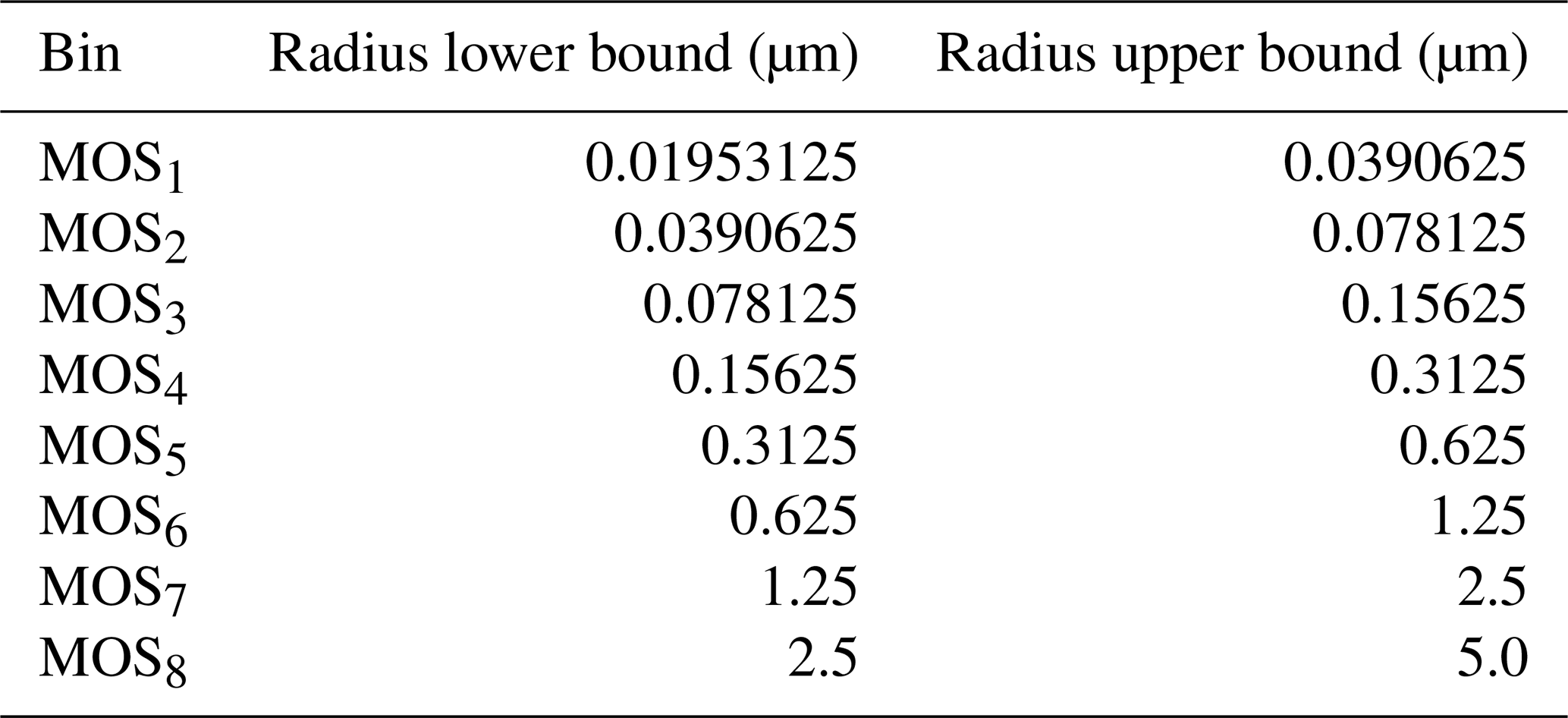
Vertical profiles of aerosol optical properties such as aerosol optical depth, single-scattering albedo, and asymmetry factor are computed by the parameterized Mie theory (Ghan and Zaveri, 2007) at 4 wavelengths (300, 400, 600, and 1000 nm). Wavelength interpolation based on Angstrom coefficients for these 3 quantities is used as input for the Rapid Radiative Transfer Model (RRTMG) Iacono et al. (2008) for shortwave and longwave radiation options (ra_lw_physics = 4 and ra_sw_physics = 4). The Mie parameterization was modified by Fast et al. (2006) and Barnard et al. (2010) for the sectional representation of the aerosol size distribution, such that the Mie subroutine requires input of ash and sulfate concentration presented in eight intervals. These intervals are identical to those used in the MOSAIC microphysical module (Zaveri et al., 2008). Therefore, we further refer to them as MOSAIC bins (MOS${}_{\mathrm{1},\mathrm{2},\mathrm{3},\mathrm{4},\mathrm{5},\mathrm{6},\mathrm{7},\mathrm{8}}$), see Table 2.

Table 2 Particle dry-radii range for the 8 size bins employed by MOSAIC.

As mentioned above, ash mass can be redistributed between 4 or 10 bins (see Table 1). Sulfate aerosol is prescribed by two log-normal distributions, which describe Aitken and accumulation modes. Parameters of these two distributions are given in Sect. 2.5. Following Stenchikov et al. (2021), we assume that the accumulation mode comprises 95 % of the sulfate mass, and the Aitken mode 5 %.

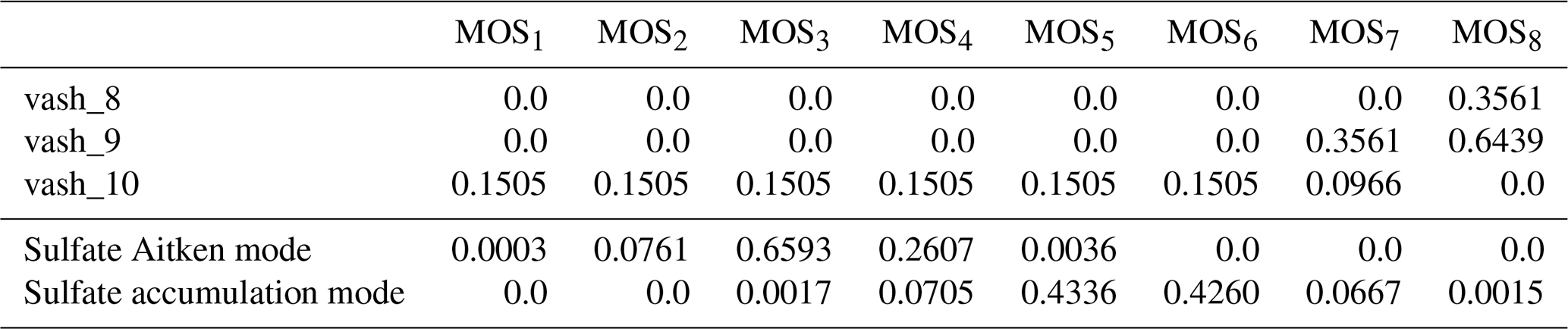
Mass of ash and sulfate is divided between MOSAIC bins before being passed into the Mie routine. Calculation of mapping coefficients for ash is done by analogy with the method in Ukhov et al. (2021). The following formula is used to calculate the mapping coefficient fr_i for sulfate aerosol for the ith MOSAIC bin with boundaries r_i and r_i+1 listed in Table 2.

$$\begin{array}{}\text{(29)}& {\mathit{\text{fr}}}_{(\mathrm{1},\mathrm{2})i}={\displaystyle \frac{{\int }_{r_i}^{r_{i+\mathrm{1}}}{r}^{\mathrm{2}}\cdot \frac{\mathrm{1}}{\ln {\mathit{\sigma }}_{\mathrm{1},\mathrm{2}}\sqrt{\mathrm{2}\mathit{\pi }}}\exp \left(-\frac{(\ln r-\ln r_{\mathrm{1},\mathrm{2}}{)}^{\mathrm{2}}}{\mathrm{2}{\ln }^{\mathrm{2}}{\mathit{\sigma }}_{\mathrm{1},\mathrm{2}}}\right)\mathrm{d}r}{{\int }_{\mathrm{0}}^{\mathrm{\infty }}{r}^{\mathrm{2}}\cdot \frac{\mathrm{1}}{\ln {\mathit{\sigma }}_{\mathrm{1},\mathrm{2}}\sqrt{\mathrm{2}\mathit{\pi }}}\exp \left(-\frac{(\ln r-\ln r_{\mathrm{1},\mathrm{2}}{)}^{\mathrm{2}}}{\mathrm{2}{\ln }^{\mathrm{2}}{\mathit{\sigma }}_{\mathrm{1},\mathrm{2}}}\right)\mathrm{d}r}}.\end{array}$$

The computed mapping coefficients for ash and sulfate are presented in Table 3. Ash bin vash_8 is only partially accounted for in MOS₈ MOSAIC bin, while the contribution of bin vash_10 spans across MOS₁ and MOS₇. We do not include in the Table 3 the contributions of the ash bins $\text{vash\_}\mathrm{1},\mathrm{2},\mathrm{\dots },\mathrm{7}$ as they are out of the MOSAIC size range and therefore not accounted for in the mass redistribution. Sulfate in Aitken mode only contributes to the MOS${}_{\mathrm{1},\mathrm{2},\mathrm{3},\mathrm{4},\mathrm{5}}$ bins; MOS${}_{\mathrm{3},\mathrm{4},\mathrm{5},\mathrm{6},\mathrm{7},\mathrm{8}}$ bins are affected by larger particles belonging to the accumulation mode.

Table 3 Ash and sulfate mass redistribution between eight MOSAIC bins.

Aerosol optical properties computed using the volume averaging mixing rule (aer_op_opt = 1) that assumes internal mixing of aerosol composition that averages the refractive indices for each MOSAIC bin (Fast et al., 2006). Within each bin, aerosol particles of each species are simplified as spheres undergoing hygroscopic growth. Volume of the water in ith bin (Vol_h2o,i) computed following to Petters and Kreidenweis (2007):

$$\begin{array}{}\text{(30)}& {\text{Vol}}_{\text{h2o},i}={\displaystyle \frac{\text{RH}}{\mathrm{1}-\text{RH}}}\cdot \left({\text{Vol}}_{\text{sulf},i}\cdot {\mathit{\kappa }}_{\text{sulf}}+{\text{Vol}}_{\text{ash},i}\cdot {\mathit{\kappa }}_{\text{ash}}\right),\end{array}$$

where RH is the relative humidity, Vol_sulf,i and Vol_ash,i are the volumes of sulfate and ash, respectively, in the ith bin. Ash hygroscopicity κ_ash=0.1 (Stuefer et al., 2013), sulfate hygroscopicity κ_sulf=0.5 (Abdul-Razzak and Ghan, 2004). Aerosol optical depth (AOD) at 300, 400, 600, and 1000 nm, as well as shortwave (SW) and longwave (LW) fluxes at the bottom and top of the atmosphere (BOA and TOA, respectively), are available in the WRF-Chem output. Calculation of volcanic aerosol radiative feedback is activated by setting aer_ra_feedback = 1 in the namelist.input file.

3 Results

Three options are available for simulating volcanic cloud dispersion: volcanic ash with 4 fine or 10 fine and coarse ash species (chem_opt = 403, chem_opt = 400), or SO₂ with 10 ash species (chem_opt = 402). The namelist parameter emiss_opt_vol defines the constituents of the eruption, i.e. at emiss_opt_vol = 1 only the emission of ash is simulated, while emiss_opt_vol = 2 also includes SO₂ emission. Here, we introduced a new option, emiss_opt_vol = 3, which, in addition to ash and SO₂, also accounts for emissions of sulfate and water vapor. This option requires that emissions be prepared only using the developed tool PrepEmisSources; see Appendix A for details. While emiss_opt_vol = 1, 2 can be used only with emissions prepared using the PREP-CHEM-SRC utility. Hereafter, we use only emiss_opt_vol = 3 and chem_opt = 402. The WRF model was configured with the Yonsei University (YSU) planetary boundary layer scheme bl_pbl_physics = 1 (Hong et al., 2006), the RRTMG longwave and shortwave radiation schemes ra_lw_physics = 4, ra_sw_physics = 4 (Iacono et al., 2008), the WSM 5-class microphysics scheme mp_physics = 4 (Hong et al., 2004), the unified Noah land-surface model sf_surface_physics = 2 (Tewari et al., 2004), and the Grell 3D cumulus parameterization cu_physics = 5 (Grell and Dévényi, 2002).

3.1 Short-term experiments

In order to verify the modifications introduced in the code and to assess the mass balance of ash, sulfate, and SO₂, a hypothetical 2 h-long Mt. Pinatubo eruption was modeled, with the total simulation period extending to 30 d (15 June to 15 July 1991). Domain dimensions are 75×40 grid-cells in zonal and meridional directions, respectively. The domain is centered at 9° N, 95° E. Grid resolution is 100 km². The meteorological initial and boundary conditions for WRF-Chem are also calculated using the ERA-Interim reanalysis product (Dee et al., 2011) provided at 0.75°×0.75° horizontal and 6 h temporal resolution. We emitted 65 Mt of ash and 15 Mt of SO₂. The emissions were redistributed following an umbrella profile spanning from 1 to 15 km, with 95 % of the mass contained within the umbrella cloud. The total emitted ash mass was evenly distributed among the ten ash size bins, with each bin assigned 10 % (fraction =0.1) of the total ash mass (refer to example3.py in Ukhov and Hoteit, 2025). The prepared emission file is being read every two hours. To avoid the volcanic debris loss through the boundary, periodic boundary conditions were imposed by setting the following parameters in the namelist.input: specified = .false., periodic_x = .true. and periodic_y = .true. .

3.1.1 Test of settling velocity of large ash particles

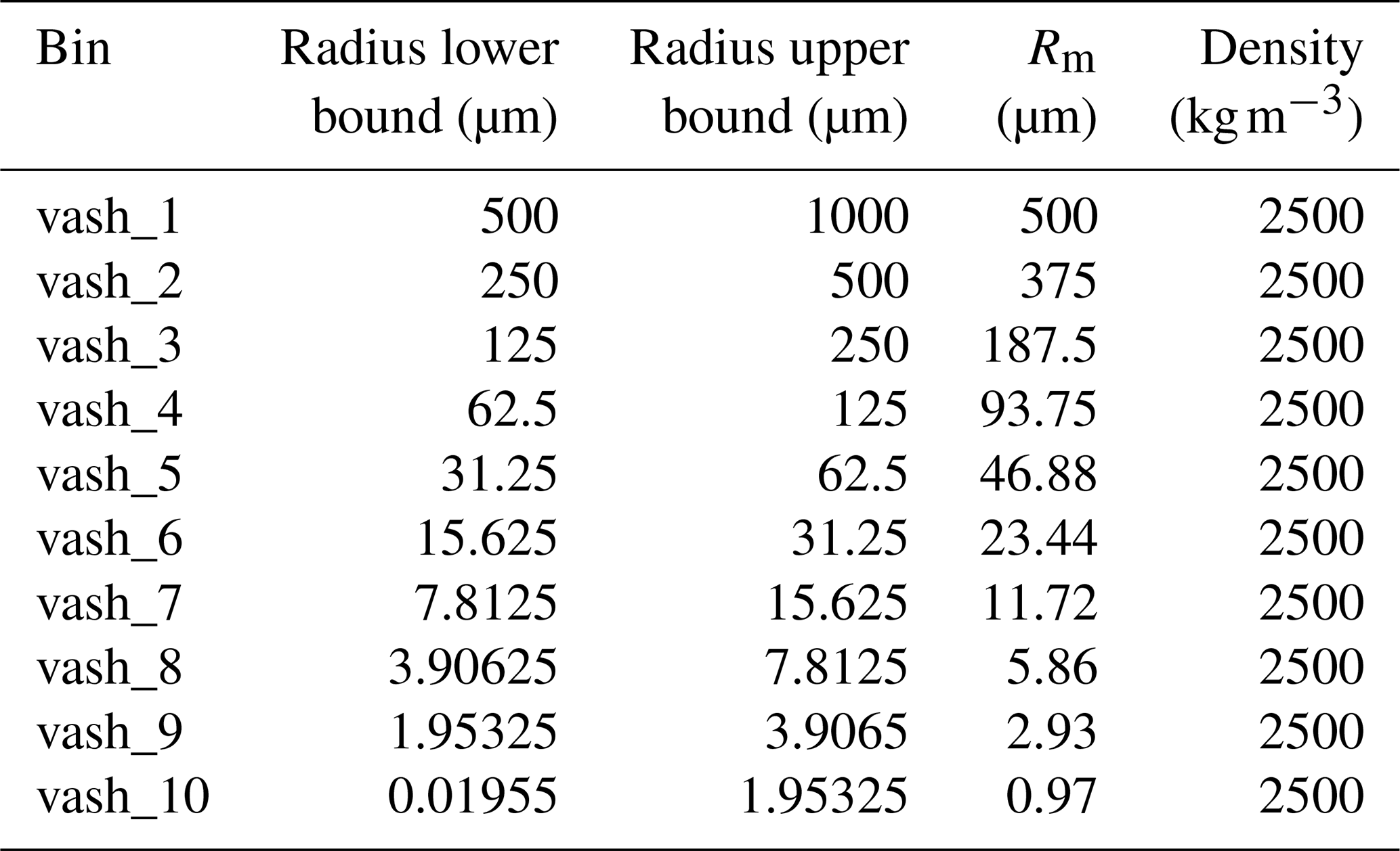
Figure 1 illustrates the settling velocities of ash particles as a function of altitude, with variations in particle radii, calculated both prior to and following the implementation of the correction factor, see Sect. 2.7.1. Gravitational settling velocity of sulfate particles having dry volume median radii =0.62 µm (see Sect. 2.5) is also shown. We compare our results with theoretical formulations by Kasten (1968) and Armienti et al. (1988). Presented in Kasten (1968), settling velocities are for spherical particles with radii of 1, 3, and 10 µm. For comparison purposes, the density of these particles was adjusted to align with that of the ash. In Armienti et al. (1988), the ranges of terminal velocities are provided for feldspar mineral particles (with radii of 23.5, 46.75, 93.75, and 187.5 µm), which are regarded as having the closest density to ash particles.

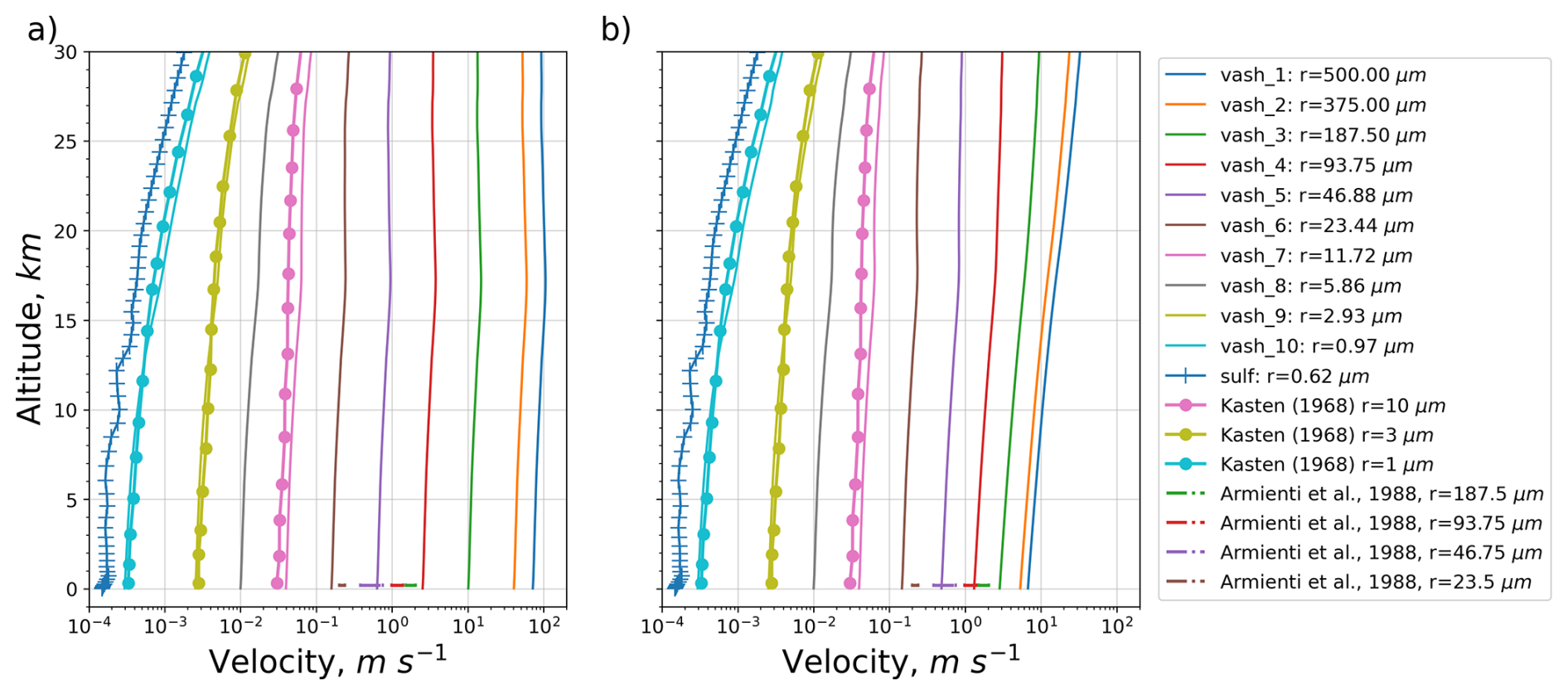
Figure 1 Settling velocity as a function of altitude computed for ash particles with different radii and sulfate particles with dry volume median radii =0.62 µm. Comparison with theoretical data by Kasten (1968) and Armienti et al. (1988). Before (a) and after (b) correction of the settling velocity of the large ash particles.

Both panels in Fig. 1 show that settling velocities are increasing as a function of particle size and increasing with altitude. Sulfate particles, possessing lower density and smaller size, exhibit the minimal settling velocity. The corresponding curve appears irregular, in contrast to the smoother curves for ash particles, due to the water uptake affecting the size and, therefore, settling velocity of sulfate particles, see Eq. (12).

Before the correction, erroneously high settling (>40 m s⁻¹) velocities are observed for the ash particles in the two largest bins. The updated plot (Fig. 1b) shows that the settling velocities of ash particles with radii ≥23.44 µm decreased across the entire altitude range compared to the original plot (Fig. 1a). This shift is particularly evident for the largest particle classes (e.g., r=500, 375, 187.5 µm), where the velocity curves move leftward, indicating slower sedimentation. Settling velocity was overestimated up to 10 times for the largest particle bin. After the correction, the velocities of large particles align more closely with those presented in Armienti et al. (1988).

3.1.2 Test of ash mass balance

To validate the rectified finite-difference scheme applied to the gravitational settling of ash (as described in Sect. 2.7.2), the model was executed twice: initially without modifications in the scheme and in the settling velocity of large particles, and subsequently with these two changes. In each scenario, the mass balance for ash was computed. Figure 2 illustrates the temporal evolution of the components of the ash mass balance derived from these two simulations. The components are: ash column loading, dry deposited ash, precipitated via large and convective scales ash, gravitationally settled ash, and the cumulative mass (sum of all components). Figure 2a shows that the amount of gravitationally settled ash (green line) increases rapidly, reaching 123 Mt after one month. This dominant sink suggests overactive ash fall. In the rectified experiment (Fig. 2b), only 53 Mt of ash is settled, which is 2.3 times less. Cumulative (loading+depos.+precip) mass (brown line) (Fig. 2a) shows a continuous increase up to 150 Mt, which significantly exceeds ash emissions (65 Mt), implying a lack of ash mass balance closure with artificial mass gain. In contrast, cumulative mass in Fig. 2b is fixed at 65 Mt, which corresponds to the emitted amount of ash and confirms ash mass conservation. The dry deposition and wet deposition (orange, red, and purple lines) remain minor contributors to the deposition process (Fig. 2a), but they are higher in comparison with the experiment with the corrected scheme (Fig. 2b).

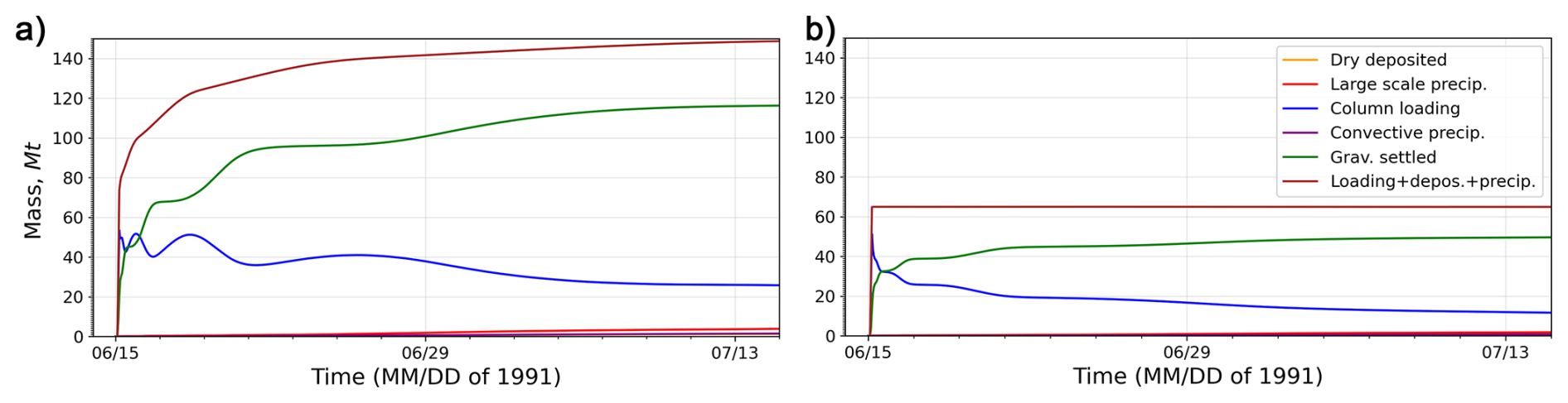
Figure 2 Ash mass balance check: before (a) and after (b) correction of the finite-difference scheme in the gravitational settling subroutine. Deposited ash includes dry deposited ash and gravitationally settled ash. Precipitated ash comprises ash scavenged by large-scale and convective-scale precipitation.

3.1.3 Test of SO₂ and sulfate mass balance

Figure 3 depicts the mass balance for SO₂ and sulfate, assuming 15 Mt of SO₂ and 5 Mt of sulfate were initially emitted following the experiment configuration described in Sect. 3.1. The computed e-folding time for SO₂ column loading equals 35.6 d, see Fig. 3a. Oxidation by OH is the dominant SO₂ sink, followed by in-cloud oxidation by H₂O₂. SO₂ dry deposition and washout by large-scale precipitation play a secondary role, at least in this configuration of emissions. The sum of all components of the mass balance matches the initial SO₂ burden (15 Mt), indicating mass conservation. Mass of sulfate increases from 5 to ≈11.5 Mt by 15 July (Fig. 3b), which indicates continuous formation from SO₂ oxidation. 7.5 Mt of sulfate formed via SO₂ oxidation; i.e., 5 Mt of SO₂ was oxidized (Fig. 3a), which corresponds to 2.5 Mt of sulfur. The amount of formed sulfate is equal to 2.5 Mt of sulfur multiplied by 3 (sulfate molar mass divided by sulfur molar mass), which is equal to 7.5 Mt. Large-scale and convective precipitation are the major sinks for sulfate below the tropopause. A separate experiment with 5 Mt of sulfate emission was run with disabled conversion of SO₂ to sulfate (by setting gaschem_onoff = 0) to validate the sulfate mass balance, see Fig. 3c. Sulfate exhibits a relatively long atmospheric residence time. Only a modest decline (≈10 %) of sulfate burden can be observed, primarily due to dry and wet deposition. The cumulative sum of all sinks and remaining burden confirms sulfate mass conservation.

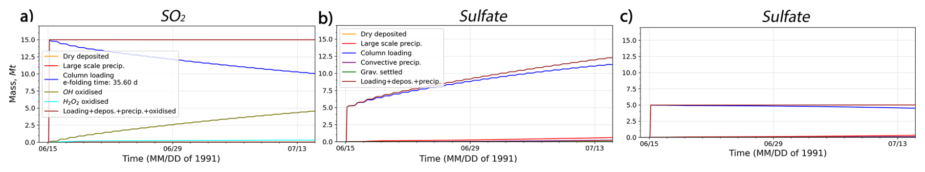
Figure 3 Mass balance: (a) SO₂ at gaschem_onoff = 1, (b) sulfate at gaschem_onoff = 1, (c) sulfate at gaschem_onoff = 0.

3.2 Long-term experiment

We conducted two 3 month simulations of the Mt. Pinatubo eruption at a 100 km grid resolution: with radiative feedback disabled (RADOFF) and enabled (RADON). Both simulations start on 15 June 1991 at 00:00 UTC. The eruption starts at 01:40 UTC and finishes at 15:40 UTC on 15 June 1991. All sinks for SO₂, sulfate, and ash mentioned above are accounted for. The dimensions of the domain are $\mathrm{376}\times \mathrm{111}\times \mathrm{60}$ points in longitude, latitude, and altitude directions, respectively, extending up to 1 hPa. The domain for the simulation is within ≈30° S–60° N latitude belt, see Fig. 8. Periodic boundary conditions on the longitudinal direction are applied by setting periodic_x = .true. in the namelist.input.

Emissions of ash and SO₂ were prepared using the developed tool PrepEmisSources (see example2.py in Ukhov and Hoteit, 2025). We used inverted time-varying emission rates of ash and SO₂ from Ukhov et al. (2023), with 66.53 Mt of ash, 15.54 Mt of SO₂ in the RADON run, and 62.67 Mt of ash, 16.73 Mt of SO₂ in the RADOFF run. Sulfate is not emitted in this experiment. We emit 100 Mt of water vapor, with 75 Mt distributed according to a parabolic profile between 17 and 12 km, and the remaining 25 Mt distributed linearly between 12 and 1 km, following Stenchikov et al. (2021). We inject water vapor to account for its radiative influence on the volcanic plume, as water vapor can modify buoyancy and radiative heating. Although we do not analyze water vapor evolution in this paper, it is included to ensure physically consistent plume thermodynamics. To determine the ash mass fractions for each bin, we follow Stenchikov et al. (2021), assuming that the ash particle size is log-normally distributed with a median radius of 2.4 µm and a geometric width of 1.8. We employed the same method as utilized for sulfate mass redistribution across MOSAIC bins, as referenced in Sect. 2.8. The computed ash mass fractions are the following: 0.0 %, 0.0 %, 0.0 %, 0.0 %, 0.5 %, 7.3 %, 32.6 %, 42.2 %, 15.8 %, 1.7 % for vash_1, vash_2, …, vash_10 bins, see Table 1. In Stenchikov et al. (2021) and Ukhov et al. (2023) we obtained the following mass fractions: 0.1 %, 1.5 %, 9.5 %, 45 %, and 43.9 % for ash bins 1 to 5, respectively.

Spectral nudging (Miguez-Macho et al., 2004) has been applied above the PBL (>5.0 km) to horizontal wind components (u and v) for the European Centre for Medium-Range Weather Forecasts Era-Interim reanalysis fields. The nudging coefficient equals 0.0001 s⁻¹. Only wavelengths larger than 450 km are nudged. This setting accounts for the realistic phase of the Quasi-Biennial Oscillation and keeps the large-scale motions close to the reanalysis, letting the model develop smaller-scale disturbances freely.

The volcanic cloud after the Mt. Pinatubo eruption was observed by several remote sensing instruments, including the total ozone mapping spectrometer (TOMS) (Guo et al., 2004) and stratospheric aerosol and gas experiment (SAGE) (Thomason, 1992). SAGE is a limb-viewing instrument that measures aerosol extinction in the stratosphere at different altitudes. The original SAGE observations have multiple gaps. Thomason (1992) filled these gaps using various techniques. We further refer to this data set as SAGE/ASAP. Infrared satellite SO₂ data provided by the TOVS/HIRS/2 (TIROS (Television Infrared Observation Satellite) Optical Vertical Sounder/High Resolution Infrared Radiation Sounder/2) sensor (Guo et al., 2004).

The next day after the eruption, the TOMS detected high levels of SO₂ loading and positive aerosol index (AI) values. The AI indicates the presence of UV-absorbing aerosols, derived from the contrast between measured and modeled radiances at two ultraviolet wavelengths. Positive AI values correspond to absorbing aerosols such as volcanic ash, whereas near-zero or negative values represent scattering aerosols or clear skies (Krotkov et al., 1999). The AI and AOD are linearly related if the volcanic cloud is relatively thin (i.e., AOD <5) (Krotkov et al., 1999; Ukhov et al., 2023). Figure 4 compares AI from the TOMS retrieval at 03:45 UTC on 16 June and AOD at 550 nm computed in the RADON and RADOFF runs at 04:00 UTC on 16 June. The spatial patterns of the AI and AOD are not similar for both runs. In Ukhov et al. (2023), a better agreement between these fields was achieved. This discrepancy may be due to different ash bin size ranges and, as a result, different redistribution of ash mass between MOSAIC bins used for the calculation of optical properties, see Sect. 2.8. However, AOD from the RADON run slightly better resembles the observed AI field in comparison with the AOD from the RADOFF run.

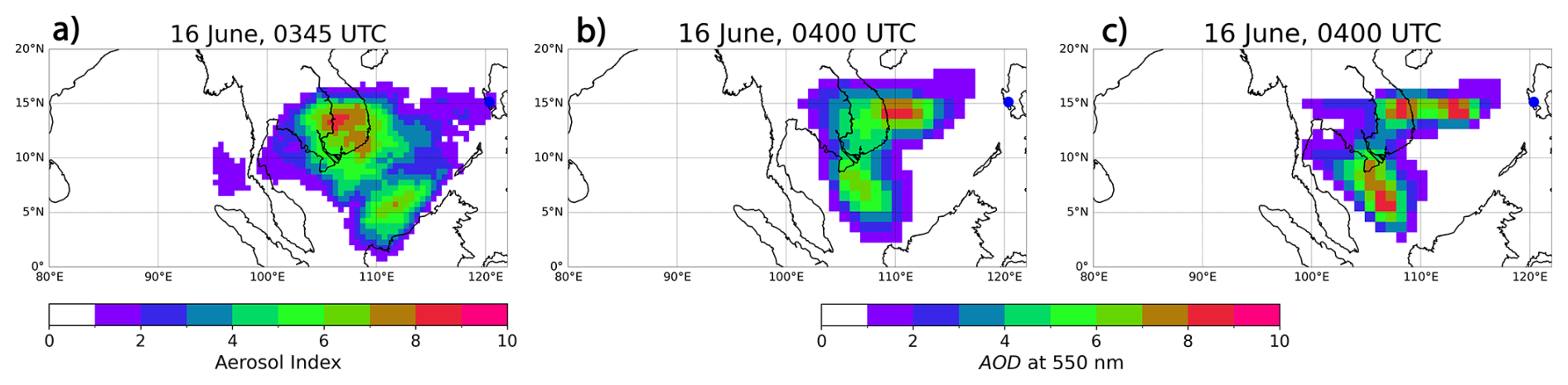
Figure 4 Observed on 16 June at 03:45 UTC and simulated aerosol diagnostics on 16 June at 04:00 UTC: (a) TOMS AI; AOD at 550 nm: (b) RADON run, (c) RADOFF run. Blue dot corresponds to the location of the Mt. Pinatubo.

Figure 5 compares observed and simulated SO₂ column loadings on 18 June, three days after the volcanic eruption. The absorption of solar radiation by volcanic ash warms the surrounding air within the ash plume, enhancing its buoyancy. This heating also modifies the plume's vertical and horizontal structure. This dynamical response in the RADON run (Fig. 5b) results in a broader SO₂ plume compared to the RADOFF run (Fig. 5c). The altered temperature gradients also modify local wind fields, slightly shifting the transport pathway of SO₂ cloud. The TOMS observations in Fig. 5a depict a dispersed SO₂ plume extending westward from the volcano, with maximum column loadings of approximately 250–300 DU. The plume shows a broad latitudinal spread, with the highest concentrations situated between 5 and 12° N. The RADON simulation (Fig. 5b) reproduces the observed westward transport of the SO₂ plume more realistically compared to the RADOFF run (Fig. 5c). The spatial extent and position of the plume in RADON align reasonably well with TOMS data, particularly in terms of latitudinal and longitudinal spread and peak loadings. However, the RADON's plume western and northern extents are slightly overestimated relative to observations. In contrast, the SO₂ plume from the RADOFF simulation (Fig. 5c) displays significant deviations from the observed plume. In particular, the RADOFF plume is split into two distinct parts: the northern part with maximum values between 400 and 450 DU, and the southern part with maximum values up to 200 DU. Overall, in contrast with the RADOFF run, the RADON experiment demonstrates a better match to the TOMS data, both in SO₂ loading magnitude and spatial distribution.

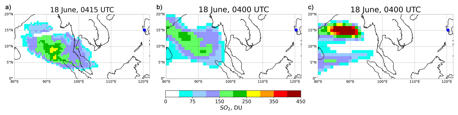
Figure 5 Observed and simulated SO₂ column loadings (DU) on 18 June. (a) The Total Ozone Mapping Spectrometer (TOMS) retrieval, simulated from the (b) RADON and (c) RADOFF runs. 1 DU $=\mathrm{2.687}\times {\mathrm{10}}^{\mathrm{20}}$ ($\mathrm{molec}.{\mathrm{m}}^{-\mathrm{2}}$). Blue dot corresponds to the location of the Mt. Pinatubo.

Figure 6 presents the temporal evolution of SO₂, sulfate, and ash mass during the first 3 months following the eruption, along with the contributions of major sinks. These diagnostics were computed for the RADON run. The initial SO₂ mass of 15.54 Mt is decreasing steadily over time. This decline is primarily driven by atmospheric oxidation processes converting SO₂ into sulfate aerosols, with an effective e-folding time ≈34 d. Minor contributions to SO₂ removal arise from dry deposition and precipitation scavenging, but these represent a small fraction of the overall loss compared to chemical transformation. The simulated rate of decay is close to the TOVS and TOMS estimates.

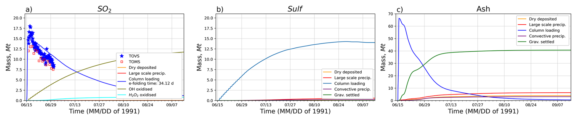
Figure 6 Temporal evolution of the mass (Mt) computed for RADON run: (a) SO₂, (b) sulfate, (c) ash, along with the contribution of corresponding sinks. TOVS (short for TOVS/HIRS/2) (Guo et al., 2004) and TOMS (Bluth et al., 1992) retrievals of SO₂ mass are shown by markers.

Sulfate mass increases as SO₂ is oxidized primarily by OH, see Fig. 6a. Sulfate mass reached about 14 Mt by the end of August. This growth reflects sustained conversion of SO₂, with a minor fraction of sulfate removed by deposition and precipitation. Ash mass dynamics (see Fig. 6c) differ from those of SO₂ and sulfate. The ash column loading shows a rapid initial decline within the first few weeks. Ash mass loss is dominated by gravitational settling and, to a lesser extent, by precipitation and dry deposition.

Figure 7 displays the ash, SO₂, and sulfate domain-averaged concentrations as a function of altitude and time computed for the RADON and RADOFF experiments. Solid lines and shading in Fig. 7 show the volcanic cloud boundary from the RADON experiment; dashed lines correspond to the RADOFF experiment. The threshold concentrations are at the color bar's lowest value. In Fig. 7a and c, ash and SO₂ are present from the beginning of the experiments. It takes about 2–3 d to produce a significant amount of SO₄. The RADON run shows a more pronounced and sustained presence of ash, SO₂, and sulfate compared to the RADOFF run, suggesting that lofting caused by the radiative heating resists gravitational settling. Despite the gravitational settling, the ash cloud rises initially before descending into the troposphere, see Fig. 7a. The SO₂ cloud, driven by buoyancy generated by the radiative heating of eruption products, moves up. In the RADOFF run, the stratospheric updrafts also move SO₂ and SO₄ up, but at a much slower pace. The gravitational settling of sulfate aerosols restricts the SO₄ cloud's upward motion. Eventually, sulfate deposition velocities define the level of neutral buoyancy for the SO₄ cloud. Differential radiative heating and gravitational settling lead to a separation of ash, SO₂, and sulfate clouds. In the RADOFF simulation, sulfate converted from SO₂ below the tropopause undergoes a separation and is rapidly deposited. During the initial two months, the sulfate cloud experiences an ascent; subsequently, it becomes diluted and stabilizes as the buoyancy weakens due to cloud dispersion. In the RADOFF experiment, the SO₂ and SO₄ clouds end up 3–4 km lower than in the RADON experiment.

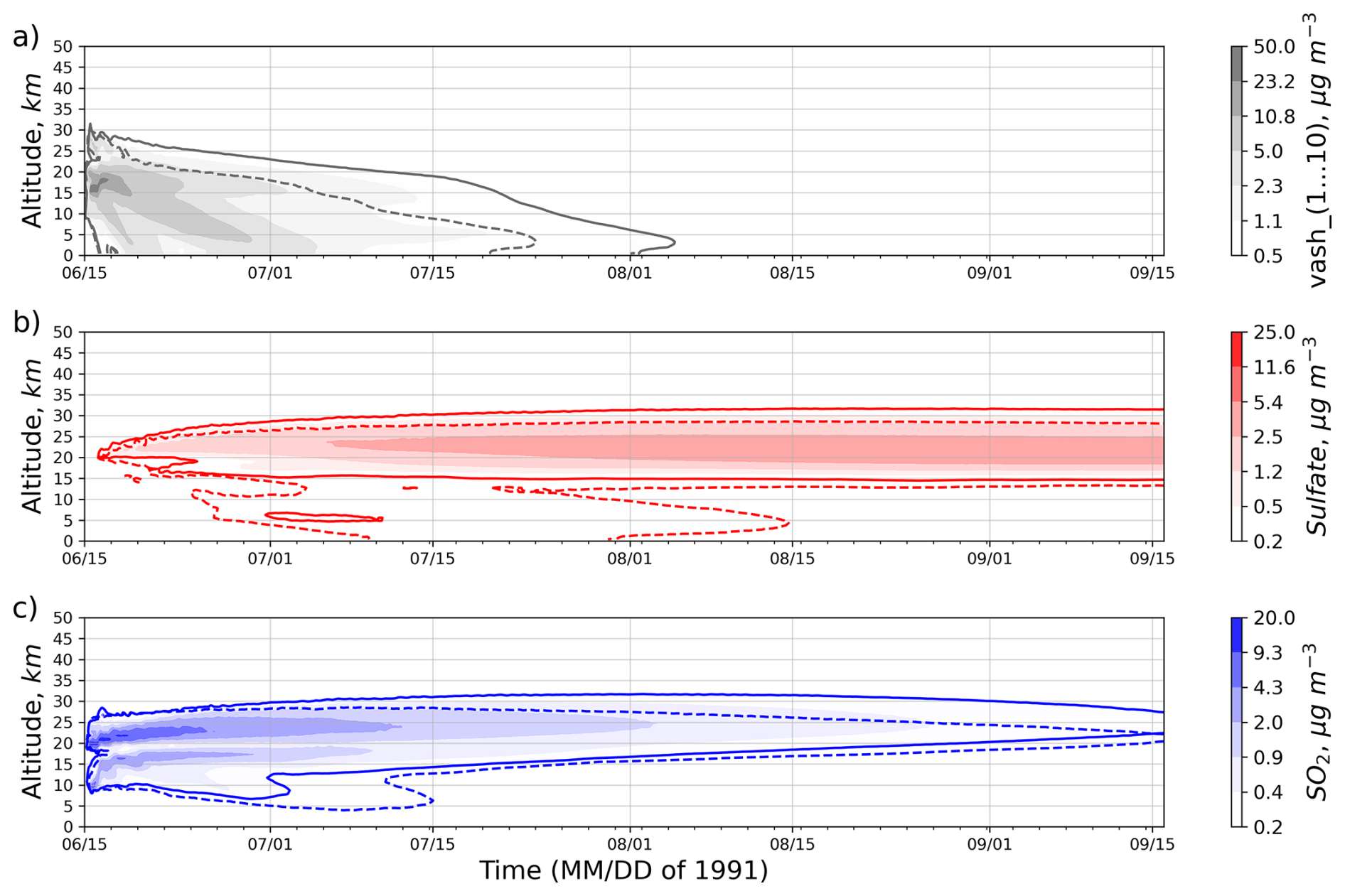
Figure 7 Hovmöller diagrams of the temporal and vertical distribution of domain-averaged concentrations (µg m⁻³): (a) ash, (b) sulfate, (c) SO₂. Solid contour lines and shading correspond to the RADON run, which incorporates enabled radiative feedback. Dashed contour lines correspond to the RADOFF run.

Figure 8 presents the accumulated deposition of ash and sulfur over 3 months following the eruption. The ash and sulfur deposition includes dry deposition, gravitational settling, and washout by large-scale and convective precipitation. The spatial pattern of ash fall is concentrated over Southeast Asia and the western Pacific, where values exceed 1 g m⁻². In general, the spatial distribution of tephra-fall deposits is in agreement with Paladio-Melosantos et al. (1996) and Wiesner et al. (1995). Ash accumulation also occurred along the equatorial zone in the Indian Ocean, central Africa. It reached the west coast of the Americas, although deposition amounts decreased progressively with distance from the source. Minimal ash fall is seen over the North Atlantic and Central Pacific, as most of the coarse ash particles settled within the first few thousand kilometers downwind. The total mass of ash deposited over the domain is 54.18 Mt, confirming that nearly 80 % of the injected ash (54.18 out of 66.53 Mt) was removed from the atmosphere within three months. This removal primarily reflects the gravitational settling of coarse ash particles (>1 µm; Stenchikov et al., 2021), whereas submicron particles remained aloft for a longer period. The accumulated sulfur deposition sums to 0.38 Mt over the same period. Given that sulfate mass reached about 14 Mt by the end of August (see Fig. 6b), and that most SO₂ had been oxidized, the deposition of 0.38 Mt of sulfur represents only a small fraction of the emitted SO₂. The deposition pattern of sulfur is more dispersed than that of ash, reflecting the widespread transport, see Fig. 8b. Sulfur fall is generally lower in magnitude, as most of the sulfate aerosol remains suspended at high altitudes and contributes to the long-lived stratospheric sulfate layer rather than being removed by deposition processes. Sulfur deposition occurred broadly across the tropical belt. Noticeable sulfur fall affected the Pacific Ocean, Central America, and Central Africa. In these areas, we expect the precipitation to be more acidic.

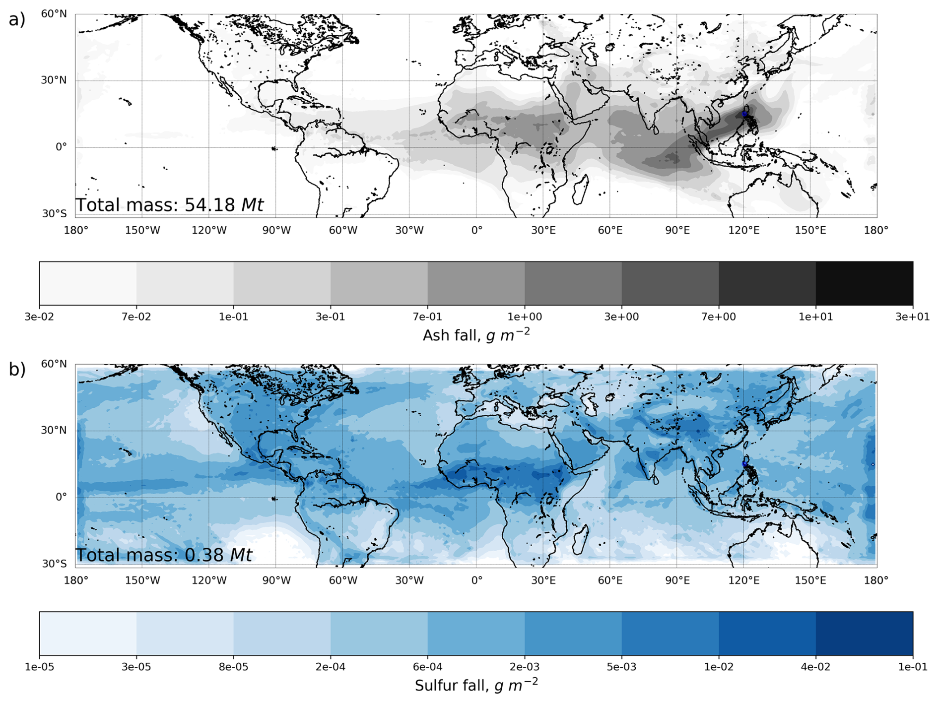
Figure 8 Accumulated fall (g m⁻²) over 3 months following the eruption: (a) ash, (b) sulfur. Dry and wet deposition contributions, including gravitational settling, and removal by large-scale and convective precipitation, is accounted for in both cases.

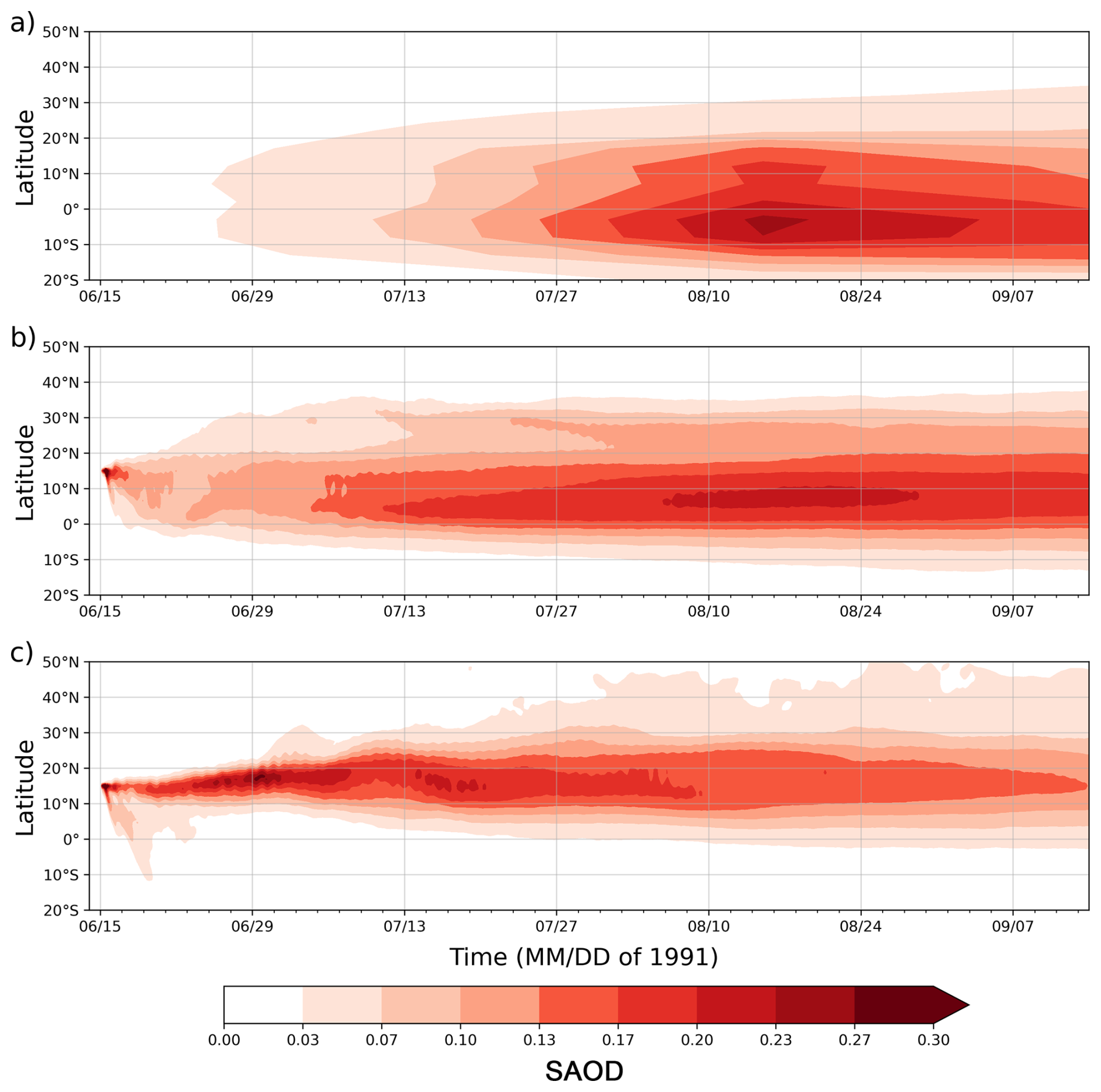
Figure 9 compares the observed (SAGE/ASAP) (Thomason, 1992) and simulated in RADON and RADOFF runs zonal mean stratospheric aerosol optical depth (SAOD), which includes contributions from ash and sulfate. In the RADOFF run, during the first week, a significant amount of aerosol moves to the Southern Hemisphere, reaching 10° S, but the maximum SAOD remains in the Northern Hemisphere. In contrast, the SAOD structure in the RADON run is close to that observed by SAGE, including the position of maximum SAOD, latitudinal spread, and pattern. But in the RADON run, the SAOD pattern is shifted by 10° to the north compared with the SAGE/ASAP observations. The maximum SAGE/ASAP SAOD is in the 10° S–0° range, whereas in the RADON run, the SAOD maximum is within the 0°–10° N range. This suggests that the RADON simulation slightly overestimates the transport of aerosols into the Northern Hemisphere, which was also observed in our previous study (Stenchikov et al., 2021).

Figure 9 Hovmöller diagrams of the zonal mean SAOD: (a) the SAGE/ASAP (Thomason, 1992) largely stratospheric AOD at 1.020 µm, (b) simulated (stratospheric and tropospheric) SAOD at 1.0 µm from RADON run, (c) same as (b) but from RADOFF run.

3.2.1 Radiative forcing of volcanic aerosol

To estimate perturbations of the Earth's radiative balance, we calculate the change of the total (SW + LW) clear-sky (effects of simulated clouds are ignored) radiative flux ΔF, at the top of the atmosphere (TOA) and at the bottom of the atmosphere (BOA), computed for perturbed (P) and control (C) runs. We define the radiative forcing (RF) as the difference in radiative fluxes:

$$\begin{array}{}\text{(31)}& {\displaystyle }\mathrm{\Delta }{F}_{\text{BOA}}=\left(F_{\text{BOA}}^{\downarrow \text{ON}}-F_{\text{BOA}}^{\uparrow \text{ON}}\right)-\left(F_{\text{BOA}}^{\downarrow \text{OFF}}-F_{\text{BOA}}^{\uparrow \text{OFF}}\right),\text{(32)}& {\displaystyle }\begin{array}{rl}\mathrm{\Delta }{F}_{\text{TOA}}& =\left(F_{\text{TOA}}^{\downarrow \text{ON}}-F_{\text{TOA}}^{\uparrow \text{ON}}\right)-\left(F_{\text{TOA}}^{\downarrow \text{OFF}}-F_{\text{TOA}}^{\uparrow \text{OFF}}\right)\\ & =F_{\text{TOA}}^{\uparrow \text{OFF}}-F_{\text{TOA}}^{\uparrow \text{ON}},\end{array}\end{array}$$

where ↓ denotes a downward flux and ↑ an upward flux. ON refers to the RADON run with activated aerosol radiative feedback, and OFF refers to the RADOFF run with disabled radiative feedback. This notation assumes that positive flux values indicate a warming effect, while negative values indicate a cooling effect. 2D fields of the SW and LW clear sky fluxes at the TOA and BOA are available in the WRF-Chem output. Zonal averaged clear sky RFs at TOA and BOA are shown in Fig. 10, and their three-month and domain-averaged values are summarized in Table 4.

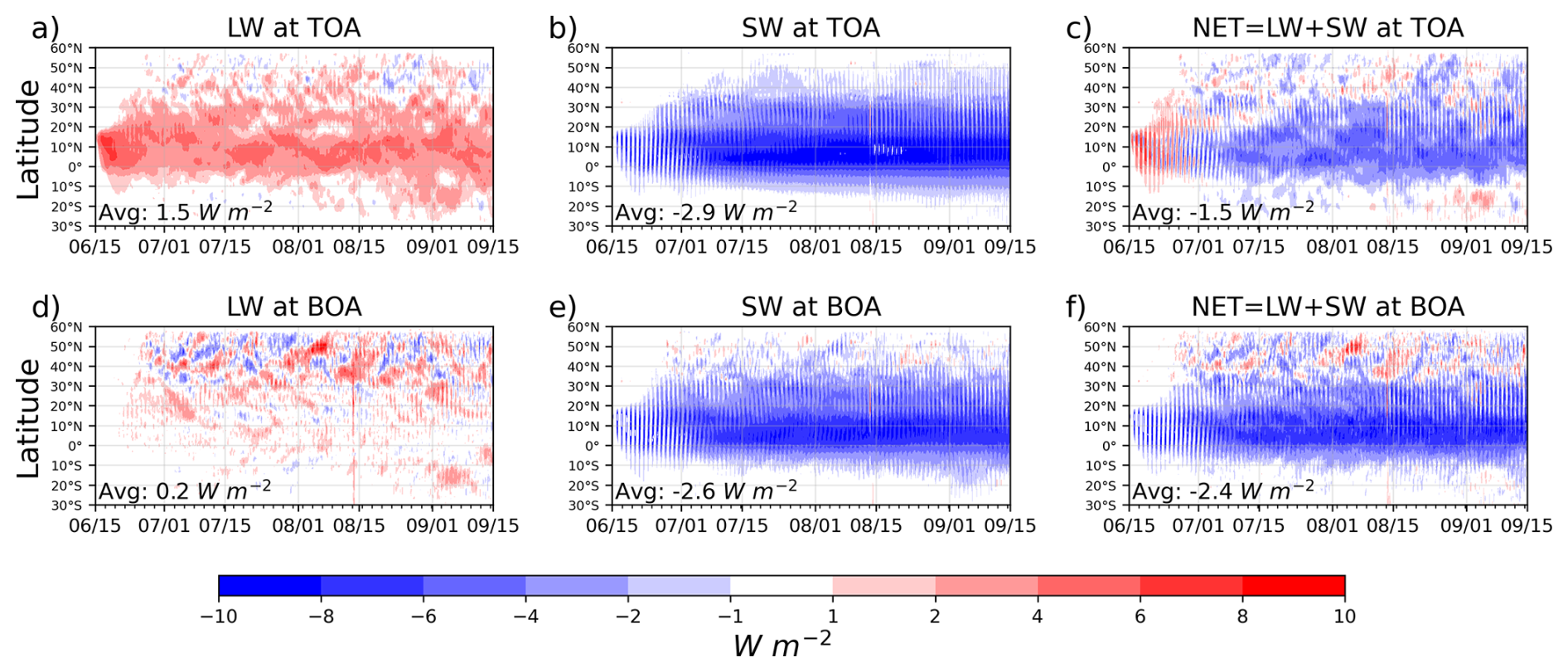
Figure 10 Hovmöller diagrams of the zonal averaged clear sky RFs for SW, LW, and $\text{NET}=\text{SW}+\text{LW}$ (W m⁻²) at TOA and BOA. Domain-averaged values of RFs are shown for each panel at the bottom right corner.

Table 4 Radiative forcings for LW, SW, and $\text{NET}=\text{LW}+\text{SW}$ (W m⁻²) at TOA and BOA three-month averaged over the simulation domain and over the globe.

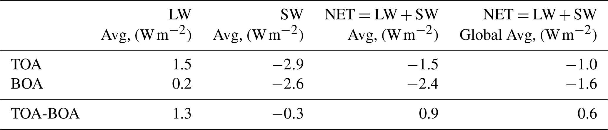
Volcanic aerosols heat both the TOA/BOA by increasing the upward/downward LW radiation from the aerosol cloud. But atmospheric absorption substantially decreases the LW perturbations at the BOA. In particular, the domain-averaged LW RF is stronger/weaker at TOA/BOA, $\mathrm{1.5}/\mathrm{0.2}$ W m⁻², respectively. Strong SW cooling dominates at TOA and BOA, domain-averaged values are −2.9 and −2.6 W m⁻², respectively. SW cooling at the TOA is caused by the sulfate aerosol's efficient scattering of solar radiation back to space. SW cooling at the BOA is conditioned by the reduced downward SW flux.

Short-lived ash particles and sulfate aerosol absorb some outgoing LW radiation, which causes warming at TOA. Simultaneously, ash and sulfate also scatter incoming SW radiation, contributing to a cooling effect, but due to the ash presence, warming at the TOA is stronger in the first two weeks. Therefore, during this period, ash dominates the $\text{NET}=\text{LW}+\text{SW}$ RF at TOA, inducing a warming at the TOA and counteracting SW cooling. After ash fallout, sulfate's SW cooling prevails over LW warming at the TOA. Calculated domain average value for NET RF at the TOA is −1.5 W m⁻², see Fig. 10c.

SW cooling prevails over LW warming at the BOA as well; domain-averaged values are −2.6 and 0.2 W m⁻², respectively. Domain average value for NET RF at the BOA is −2.4 W m⁻². Over the large areas in the equatorial zone, NET cooling at the BOA reaches −6 to −8 W m⁻², see Fig. 10f. These values of RFs are in good agreement with other modeling studies (Stenchikov et al., 1998; Ramachandran et al., 2000).

The simulation domain covers approximately 68.3 % of the globe. Therefore, to compute the global average RFs, we multiply the domain average RF value by 0.683, see the right column of Table 4. Thus, the global average $\text{NET}=\text{LW}+\text{SW}$ clear-sky RF is −1.0 and −1.6 W m⁻² at TOA, BOA, respectively.

Difference of the NET fluxes at the TOA and BOA reflects the change of the total radiative balance of the whole atmospheric column, where a positive difference of TOA and BOA (domain and global average values are 0.9 and 0.6 W m⁻², respectively) represents the heating of the part of the atmospheric column, where the sulfate aerosol cloud resides. Again, this heating is driven by the LW adsorption by sulfate aerosols.

4 Conclusions

In this study, we enhanced the WRF-Chem v4.8 model by implementing physical and chemical mechanisms that are necessary to simulate the realistic evolution of the volcanic clouds in the atmosphere. In particular, we corrected the derivation of the finite difference scheme for the gravitational settling of the ash. Specifically, ash mass balance was strongly violated in the previous WRF-Chem model runs. To the authors' knowledge, the found inconsistency, despite the long-term usage, has not previously been recognized or reported. We also introduced the correction factor for the deposition velocity for coarse ash particles (radii ≥23.44 µm). We refined SO₂ oxidation processes and implemented gravitational settling for sulfate aerosols, which is important for volcanic stratospheric clouds and was previously neglected. We implemented an interaction of ash and sulfate aerosols with SW and LW radiation. This so-called direct radiative effect of aerosols refers to the radiation changes caused by aerosol absorption and scattering. In general, our modifications and additions provide a more physically consistent representation of volcanic plume dynamics and will improve volcanic ash and SO₂ forecasts, benefiting both scientific research and operational applications. Additionally, we developed an open-source preprocessor called PrepEmisSources, see Appendix A and Ukhov and Hoteit (2025) for details. This tool facilitates the preparation of the volcanic emission file used by WRF-Chem, and emissions can be time varying. For this, we introduced a new option emiss_opt_vol = 3 which, besides ash and SO₂, also accounts for emissions of sulfate and water vapor. All these new capabilities are available under chem_opt = 402 option in the namelist.input file. Therefore, we encourage using the PrepEmisSources utility along with emiss_opt_vol = 3, which can be used with chem_opt = 402, 400, or 403.

We demonstrate the effect of changes implemented into the WRF-Chem v4.8 model by running one short-term and two long-term experiments (with enabled and disabled radiative feedback, respectively), which simulate the Mt. Pinatubo eruption. In all experiments, the emissions were prepared using the developed PrepEmisSources utility. In the former run, we successfully established the mass balance for ash, SO₂, and sulfate, accounting for all major sinks by prescribing periodic boundary conditions to avoid mass loss through the lateral domain boundaries. Using the long-term runs, we estimated the role of the radiative heating, traced the spatio-temporal evolution of the AOD and distributions of the ash and sulfate clouds, and calculated the maps of ash and sulfur fallout. Where possible, the results of the simulations were compared with the observations.

We found that the radiative effect of eruption products improves the model's ability to predict the transport of volcanic clouds and increases their persistence in the atmosphere. The interaction of the aerosols with atmospheric radiation through scattering and absorption was also significant and resulted in cooler surface temperatures. In particular, in the equatorial area, the net cooling at the BOA reaches −6 to −8 W m⁻², which is within the acknowledged range shown in other studies. In the long-term experiment, the model captured the transition from ash-dominated to sulfate-dominated forcing at the TOA. Just after the eruption, the ash radiative forcing dominates over the weak sulfate radiative forcing, which strengthens after two weeks when enough sulfate mass has formed.

We demonstrated that the enhanced WRF-Chem v4.8 model could be useful in multiple applications. Starting from the simulation of the impact of volcanic clouds on aviation and forecasting ash and sulfur fallout, and finishing by calculating the volcanic cloud's effect on climate. We hope that the new additions and rigorous validation provided in this paper could help promote the WRF-Chem v4.8 to the cohort of the VATD models used by VAACs.

This work is in line with the open-source paradigm and will help WRF-Chem users to better handle the code and understand physical interconnections. In the course of the paper, we tried to designate places in the code where we implemented changes and where the model parameters can be changed. As the adjustments for the specific eruption might need to be made. Firstly: ash size distribution, refractive index, and ash density. Secondly, the sulfate size distribution parameters for both modes.

5 Future work

Recently, one of the directions of geoengineering modeling, such as Stratospheric Aerosol Injection (SAI), has become popular. The idea behind SAI is mimicking the cooling effects of volcanic eruptions by injecting aerosols into the stratosphere, where they would scatter some incoming shortwave radiation and cool the Earth's surface. Recent research (Stefanetti et al., 2024) suggests that solid particles, such as diamond, could be used as these aerosol particles. It was shown that diamond is most efficient in reducing global warming per unit injection. In contrast to sulfate aerosols, it has fewer side effects, such as less absorption of terrestrial infrared radiation, which results in stratospheric warming and reduced cooling efficiency. In addition, diamond is a chemically inert material, which does not cause ozone depletion. We would like to note that in its current configuration, the enhanced WRF-Chem v4.8 model could be potentially used for the simulation of SAI and studying its effects on climate, at least using diamonds as injected material. Inclusion into the model calculation of the heating rates by analogy with the Stenchikov et al. (2021) would provide a better view of the vertical redistribution of cooling and warming within the atmospheric column. Adding the “double call” method (Stenchikov et al., 1998) into the radiation calculation would allow for the separate calculation of the radiative forcings for ash, sulfate, and water vapor (Stenchikov et al., 2025). The next step in further enhancing the code would be adding a relevant chemical mechanism using the kinetic preprocessor (KPP) (Damian et al., 2002) for the simulation of stratospheric or tropospheric chemical reactions, including the photolysis reactions. Ash aggregation, sulfate nucleation, interactions between sulfate and ash, and heterogeneous sulfate removal via adsorption on ash surfaces are not accounted for in this version. Inclusion of these processes into the model would be a natural extension of this work. Owing to its modular design and flexibility, the developed PrepEmisSources code can be easily extended to simulate emissions of different types. For example, emissions caused by industrial or wildfires.

Appendix A: PrepEmisSources utility

The default methodology for preparing the volcanic emissions file comprises two distinct stages. Initially, it is necessary to employ an open-source tool, PREP-CHEM-SRC (Freitas et al., 2011), with a limited set of options pertinent to the parameters governing the eruption itself. In the subsequent stage, a utility program convert_emiss.exe embedded within the WRF-Chem code must be executed. This utility program reads the intermediate binary data file generated by PREP-CHEM-SRC and computes the vertical mass distribution and the emissions for the volcanic ash and SO₂. Then, computed arrays are stored in the WRF-Chem emission file. During the WRF-Chem's runtime, the emission file is processed a single time at the onset of the simulation; consequently, it becomes impossible to delineate emissions that vary temporally. Moreover, the dispersion of emissions vertically is restricted exclusively to a $\mathrm{75}/\mathrm{25}$ umbrella-shaped plume, where 25 % of the mass is distributed from vent height to a ≈73 % of plume height, while 75 % follows a parabolic distribution to plume-top height.

In order to streamline and refine the preparation of volcanic emissions, we have developed the PrepEmisSources utility. This tool, implemented in Python, is specifically designed to prepare and visualize volcanic emission scenarios for integration with atmospheric models such as WRF-Chem. The utility enables the construction of 4D (space–time-altitude) emission profiles with configurable spatial, temporal, and vertical resolutions. It supports multiple emission types (e.g., ash, SO₂, sulfate, water vapor) and vertical distribution types (e.g., uniform, umbrella, Suzuki; Suzuki, 1983; Mastin and Van Eaton, 2020), and can accommodate both synthetic and inversion-derived emission scenarios (Ukhov et al., 2023; Brodtkorb et al., 2024). With its object-oriented and extensible architecture, PrepEmisSources allows for flexible scenario definition and integration of external data. Emission profiles are exported to NetCDF files in a format directly compatible with WRF-Chem input requirements, facilitating seamless simulation of volcanic events. Visualization tools are included for diagnostic analysis of emission structures before model execution.

To accommodate the capability to read the emissions at specific intervals, we implemented changes in the WRF-Chem's logic of reading the emission file via auxiliary input 13. In particular, the emission file will be read by the WRF-Chem at uniform time intervals (namelist parameter auxinput13_interval_m in minutes) and a prescribed number of times (namelist parameter frames_per_auxinput13). This option works when chem_opt = 400, 402 or 403 and emis_opt_vol = 3. More details on how to use the PrepEmisSources utility are presented in Appendix A and in Ukhov and Hoteit (2025).

Appendix B: List of output diagnostics

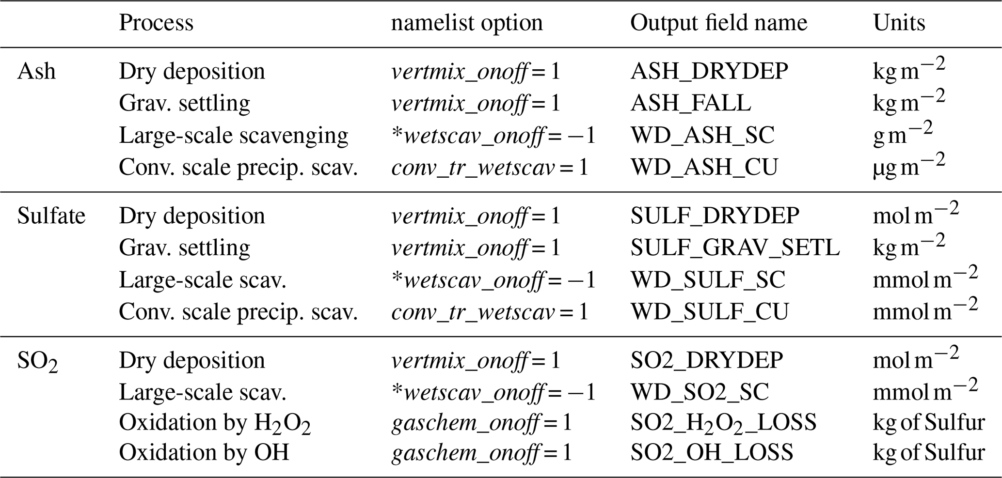
Table B1 List of output diagnostics and corresponding namelist options.

* does not work with cu_physics = 3 or 10. In our case cu_physics = 5.