Standardising the “Gregory method” for calculating equilibrium climate sensitivity

The equilibrium climate sensitivity (ECS) – the equilibrium global mean temperature response to a doubling of atmospheric CO₂ – is a high-profile metric for quantifying the Earth system's response to human-induced climate change. A widely applied approach to estimating the ECS is the “Gregory method” (Gregory et al., 2004), which uses an ordinary least squares (OLS) regression between the net radiative flux, N, and surface air temperature anomalies, ΔT, from a 150 year experiment in which atmospheric CO₂ concentrations are quadrupled. The ECS is determined by extrapolating the linear fit to N=0, i.e. the ΔT-intercept, indicating the point at which the system is back in equilibrium. This method has been used to compare ECS estimates across the CMIP5 and CMIP6 ensembles and will likely be a key diagnostic for CMIP7. Despite its widespread application, there is little consistency or transparency between studies in how the climate model data is processed prior to the regression, leading to potential discrepancies in ECS estimates. We identify 32 alternative data processing pathways, varying by differences in global mean weighting, net radiative flux variable, anomaly calculation method, and linear regression fit. Using 44 CMIP6 models, we systematically assess the impact of these choices on ECS estimates and calculate uncertainty ranges using two bootstrap approaches. While the inter-model ECS range is insensitive to the data processing pathway, individual outlier models exhibit notable differences. Approximating a model's native grid cell area (if irregular) with cosine of the latitude can decrease the ECS by 11 %, the choice of N-variable can change the ECS by 6 %, and some anomaly calculation methods can introduce spurious temporal correlations in the processed data. Beyond data processing choices, we also evaluate an alternative linear regression method – total least squares (TLS) – which has a more statistically robust basis than OLS. However, for consistency with previous literature, and given TLS may reduce the ECS compared to OLS (by up to 24 %), thereby making a known bias in the Gregory method worse, we do not feel there is sufficient clarity to recommend a transition to TLS in all cases. To improve reproducibility and comparability in future studies, we recommend a standardised Gregory method: weighting the global mean by cell area, using the top of the atmosphere (as opposed to the top of model) N-variable, and calculating anomalies by first applying a rolling average to the preindustrial control timeseries then subtracting from the raw CO₂ quadrupling experiment. This approach accounts for model drift while reducing noise in the data to best meet the pre-conditions of the linear regression. While CMIP6 results of the multi-model mean ECS appear insensitive to these processing choices, similar assumptions may not hold for CMIP7, underscoring the need for standardised data preparation in future climate sensitivity assessments.

1 Introduction

The equilibrium climate sensitivity (ECS) – the steady state global mean surface temperature response to a doubling of atmospheric CO₂ relative to preindustrial levels – has long been a cornerstone metric for quantifying future climate change (Sherwood et al., 2020). The ECS is commonly estimated using climate models, with Charney et al. (National Research Council, 1979) first proposing a range of 1.5 to 4.5 K, based primarily on a three dimensional atmospheric circulation model. The most recent climate model-based estimate uses the model range of the coupled model intercomparison project phase six (CMIP6), placing the ECS between 1.8 to 5.6 K (Zelinka et al., 2020). Meanwhile, the Intergovernmental Panel on Climate Change (IPCC) Sixth Assessment Report (AR6) uses multiple lines of evidence to arrive at the conclusion the ECS is between 2 to 5 K with 95 % confidence (Forster et al., 2021; Sherwood et al., 2020).

The most direct method for calculating the ECS involves Earth system models (ESMs) simulating the climate until it reaches thermal equilibrium following a doubling of atmospheric CO₂. However, such an experiment is computationally expensive and it can take multiple millennia of simulation years for a model to equilibrate (Rugenstein et al., 2020). Previously, researchers often relied on the less computationally expensive atmospheric general circulation models coupled with a motionless upper ocean mixed layer, or “slab ocean”. This approach, however, can affect the ECS estimate because it excludes the effects of thermal inertia and the dynamic and thermodynamic responses of the mixed layer (Boer and Yu, 2003; Danabasoglu and Gent, 2009).

Since 2004, coupled atmosphere–ocean ESMs have been used instead to estimate the ECS using the “Gregory Method” (Gregory et al., 2004), hereafter GM, which allows for an estimate of the ECS from abrupt CO₂ perturbation simulations that are centuries rather than millennia in duration. Hereafter we use the term ECS, noting that many researchers refer to the metric calculated using the GM as the effective climate sensitivity (Caldwell et al., 2016; Dunne et al., 2020; Rugenstein et al., 2020; Rugenstein and Armour, 2021; Sanderson and Rugenstein, 2022; Zelinka et al., 2020), given that the model has not run to true equilibrium. However, we use the term ECS and leave it up to the reader to decide whether this calculation results in the equilibrium or effective climate sensitivity. Our conclusions are independent of this choice.

The GM is based on the zero-dimensional energy balance model, which relates the global mean net radiative flux anomaly at the top of the atmosphere, N, to the global mean effective radiative forcing, F, and the global mean radiative response, λΔT, where λ is the global mean feedback factor, and ΔT is the global mean near surface air temperature change relative to preindustrial levels:

$$\begin{array}{}\text{(1)}& N=F-\mathit{\lambda }\mathrm{\Delta }T\end{array}$$

To calculate the ECS using a coupled climate model, Gregory et al. (2004) take the first 90 years – standard practice has since become 150 years – of an abrupt CO₂ quadrupling experiment (abrupt-4xCO₂) relative to the model's preindustrial control experiment (piControl) and calculate an ordinary least squares (OLS) linear regression of annual mean values of N against ΔT. The steady state – equilibrium – is estimated at N=0, i.e. at the ΔT-intercept. The radiative forcing is, according to this model, the N-intercept, and the feedback factor is the (negative) slope of the regression. To express the ECS and radiative forcing relative to a doubling of CO₂ rather than a quadrupling, the ΔT- and N-intercepts are divided by two, as per the original study. Note that scaling by a factor of two implicitly assumes the forcing due to a quadrupling of CO₂ is twice that of a CO₂ doubling, which does not exactly hold if the relationship between forcing and CO₂ concentrations is not logarithmic (Byrne and Goldblatt, 2014; Etminan et al., 2016; Meinshausen et al., 2020).

The popularity of the GM is likely due to its relative simplicity, offering a linear relationship that allows for a single calculation to estimate the ECS, radiative forcing, and feedback parameter. Moreover, the GM does not require highly specific experiment configurations often needed for estimating the forcing term, such as those with fixed sea surface temperatures (SSTs) or atmospheric model intercomparison project (AMIP)-style setups (such as using SST or sea ice observations). The accuracy of the GM in estimating the three variables of interest is subject to debate (e.g. Andrews et al., 2012; Forster et al., 2016; Rugenstein et al., 2020; Rugenstein and Armour, 2021; Smith et al., 2020), particularly regarding the extent of the linear assumptions and the interpretation of the forcing term. For example, in radiative forcing specific studies, the forcing term is usually estimated from the first 20 or 30 years of data (Forster et al., 2016), rather than the full 150 years more commonly used in climate sensitivity studies. These uncertainties are why we concentrate here primarily on the ECS and feedback parameter. This study focuses on the practical application of the GM, leaving discussions about its widespread use in literature, as well as its strengths and weaknesses, to other work.

The GM is extensively used and cited across literature. It has been applied to assess CMIP5 and CMIP6 (Andrews et al., 2012; Caldwell et al., 2016; Forster et al., 2013; Zelinka et al., 2020), to investigate ECS state dependence, e.g. (Andrews et al., 2015; Armour et al., 2013; Bloch-Johnson et al., 2021; Dai et al., 2020; Dunne et al., 2020; Mitevski et al., 2023), and as a reference method for comparing climate sensitivity estimates based on alternate lines of evidence, such as observations, historical simulations, or palaeoclimate data (Chao and Dessler, 2021; Sherwood et al., 2020). While the GM calculation is relatively simple, several choices must be made during data preparation. Here we define “data preparation” as the processing steps applied to the data before performing the N–ΔT regression. Many studies lack transparency regarding these preparatory steps, leading to potential inconsistencies, amplified by the fact that Gregory et al. (2004) included limited descriptions of data preparation steps in their study. To our knowledge, no study has to date systematically assessed how different data preparation methods may influence ECS results.

Many researchers do not describe their data preparation entirely, instead presenting the ECS estimate as a direct result of the N–ΔT regression over the 150 year timeseries (Dessler and Forster, 2018; Geoffroy et al., 2013; Klocke et al., 2013; Lutsko et al., 2022; Meehl et al., 2020; Mitevski et al., 2021, 2023; Nijsse et al., 2020; Ringer et al., 2014; Zhou et al., 2021). Others provide only limited details, such as specifying the model ensemble member used (Wang et al., 2025; Zelinka et al., 2013).

Among studies that address N and ΔT data preparation, the focus typically centres on anomaly calculations and methods to account for model drift. In its simplest form, the term “anomaly” refers to the difference between the corresponding abrupt-4xCO₂ and piControl timeseries. However, methods for calculating anomalies vary widely, including applying a rolling mean (Caldwell et al., 2016; Eiselt and Graversen, 2023; Po-Chedley et al., 2018; Qu et al., 2018; Zelinka et al., 2020), linear trend (Andrews et al., 2012; Armour, 2017; Bloch-Johnson et al., 2021; Dong et al., 2020; Flynn and Mauritsen, 2020; Forster et al., 2013), or long-term average (Chao and Dessler, 2021; Jain et al., 2021; Rugenstein and Armour, 2021) to the piControl prior to subtracting from the abrupt-4xCO₂ experiment.

Given the lack of transparency and consistency across literature, we aim to investigate how different choices in data preparation may influence the ECS, radiative forcing, and feedback estimates across CMIP6 models – with a particular focus on the ECS values. We identify 32 paths, split into 16 data processing choices and two linear regression methods (Fig. 1): OLS, to be consistent with the literature and the original study (Gregory et al., 2004), and total least squares (TLS), given that it is not obvious that all the pre-conditions for OLS are met within the GM. The key difference between the two methods is that OLS requires the choice of an independent variable, and TLS does not assume independence in either variable.

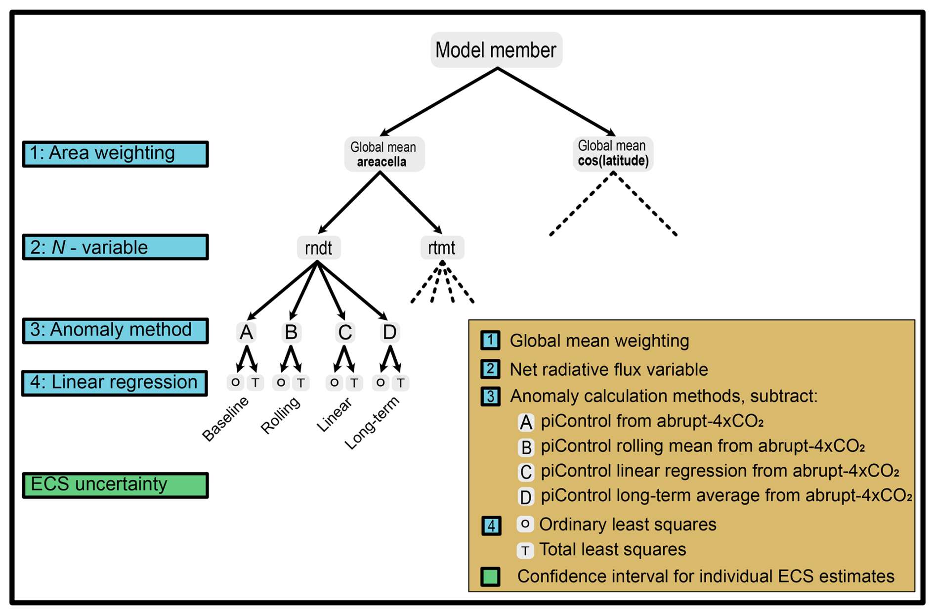
Figure 1 Decision tree illustrating the four steps and possible choices that we compare in this study in addition to the ECS uncertainty calculation. For simplicity, we have not shown all paths, although these are indicated by the dashed lines. The Baseline, Rolling, Linear and Long-term paths form the basis for much of our comparison, although we investigate the differences between all paths.

Notwithstanding the linear fit method, we do not include modifications to the regression itself. While we assess the exclusion of early years of the experiment as a further analysis in investigating ECS uncertainty (see Sect. 3.5), we do not include this as a formal data preparation step. Adjustments to the GM regression, such as excluding the initial decades of the timeseries to account for inconstant feedbacks (Andrews et al., 2015; Dunne et al., 2020), including higher order terms in the energy balance equation (Bloch-Johnson et al., 2015), or applying a non-linear ECS scaling factor between abrupt-4xCO₂ and -2xCO₂ experiments (Dai et al., 2020), are already well-documented and these studies are widely cited across the literature.

This study does not aim to constrain the ECS ensemble range. Instead, our focus is on comparing differences in data preparation and linear regression methods, exploring uncertainty, and establishing a standardised GM analysis approach. This approach aims to promote transparency in methods for future research. These objectives are particularly relevant with the upcoming release of CMIP7 data (Dunne et al., 2025), as ECS calculations will likely be among the first steps taken to compare CMIP7 models and assess how the ensemble aligns with previous CMIP generations.

2 Methods

For our analysis, we compare the effects of data preparation choices and linear regression methods across 44 CMIP6 models. The resolution and grids of the models vary (see detailed descriptions in Table S1 in the Supplement). The grid spacing is between 100 and 500 km, and the grids are either a regular latitude and longitude or a more complicated irregular (native) grid. These differences between models motivates the need to assess different global mean weighting methods.

To calculate the ECS based on the steps we investigate, the GM requires six variables, the 2 m surface air temperature (tas), top of model (TOM) net radiative flux (rtmt) and – for comparison to rtmt – top of the atmosphere (TOA) reflected shortwave radiation (rsut), TOA outgoing longwave radiation (rlut), and TOA downward shortwave radiation (rsdt). Those variables are at monthly timescales for both the abrupt-4xCO₂ and piControl experiments, and in addition, the atmospheric cell area spatial variable (areacella) is needed.

It is essential for studies using CMIP6 data to be explicit about which variables are being used in their methods. This is especially necessary for climate sensitivity research to clarify whether the ECS is an estimate of the global mean surface or global mean surface air temperature – GMST or GSAT, respectively. GSAT refers to the global 2 m air temperature, whereas GMST is a combination of 2 m air temperature over land, and SSTs over the ocean (Forster et al., 2021), which requires three variables in addition to tas to account for SSTs and sea ice concentrations (Cowtan et al., 2015). Some climate sensitivity studies are explicit about calculating the GSAT for ECS, e.g. (Andrews et al., 2015; Dai et al., 2020; Eiselt and Graversen, 2023; Gregory et al., 2004; Jain et al., 2021; Rugenstein et al., 2020; Zelinka et al., 2020), while others make the distinction between GMST and GSAT explicitly (Armour et al., 2013; Ceppi and Gregory, 2019; Geoffroy et al., 2013; Nijsse et al., 2020; Po-Chedley et al., 2018; Zhou et al., 2021). However, many (Caldwell et al., 2016; Flynn and Mauritsen, 2020; Forster et al., 2013; Klocke et al., 2013; Mitevski et al., 2021; Ringer et al., 2014; Rugenstein and Armour, 2021) refer to the ECS as a measure of GMST without describing the variables or methods used to calculate the global mean. Different methods exist to calculate the GMST from climate model data (Cowtan et al., 2015), generally diverging in their treatment of sea ice, with each method introducing potential biases (Richardson et al., 2016, 2018). It would be a step forward if studies that base their ECS derivations on GMST were explicit with their methods of global mean calculation. Given that Gregory et al. (2004) use GSAT and the IPCC recommends model-based estimates use GSAT (Forster et al., 2021), we recommend calculating the ECS using GSAT rather than GMST.

For this study, we investigate 16 data preparation paths based on choices of global mean weighting, net radiative flux variable, and anomaly calculation method (Fig. 1). These paths lead to two ECS estimates based on either OLS or TLS, which we also use to assess uncertainty in ECS for individual models. While we compare all 16 paths, for simplicity we label only four of them according to their anomaly calculation methods (Fig. 1).

We acknowledge that the choices and order of steps we identify in this study may not align with the steps taken by other researchers. However, given the lack of methodological details in some studies, and given the number of data processing choices and different orders in the lead up to the regression analysis, it is important to be clear about the exact path taken in any study.

In the following, we describe the choices at each data processing step. We include only one member for each model, prioritising the first ensemble member where possible (Wang et al., 2025; Zelinka et al., 2013). The model ensemble member describes the attributes for each experiment's specific run. The attributes relate to the realisation (r), initialisation (i), physics (p), and forcing (f) indices. Most models have at least one ensemble member called “r1i1p1f1”, whereas a model which runs two experiments of the same scenario with the same initial conditions, physics, and forcing, would then also have, in theory, an ensemble member called “r2i1p1f1”. The attributes change depending on the indices of the specific run.

To calculate the global mean, we compare two common approaches, weighting by grid-cell area or by cosine of the latitude, cos(lat). After this step we also calculate the annual mean, although this is not included as a formal step in our investigation. We choose to use an annual mean (rather than the mean of a longer time period), which is consistent with much of the literature including the original Gregory et al. (2004) study. We analyse two annual mean weighting choices: weighting each month equally or each month by the number of days. However, we find the median multi-model ECS difference between these two choices is 0.005 K, and the maximum difference is 0.023 K for CESM2-FV2. Given the ECS appears almost entirely insensitive to the annual mean weighting across all models, we do not include this as a distinct comparison in our analysis.

For the N-variable, most studies lack detail on how they calculate the net radiative flux. In our analysis, we explore approaches which either define N as a measure of the TOA $\text{rndt}=\text{rsdt}-\text{rsut}-\text{rlut}$ (Lewis and Curry, 2018), or as the explicit TOM radiative flux variable (rtmt). While we are unfamiliar with the rtmt variable's use in climate sensitivity literature, it is worthwhile to investigate especially if there are large differences between a model's explicit top and the TOA.

To calculate the anomalies, we compare four approaches which reflect the methods used across the literature, which we label as:

• A.

  Baseline: Subtract each year of the piControl from the contemporaneous abrupt-4xCO₂ timeseries. Despite this method not explicitly appearing in the literature, we include it here given the number of papers which cite anomalies with no method described (Dessler and Forster, 2018; Klocke et al., 2013; Lutsko et al., 2022; Meehl et al., 2020; Mitevski et al., 2021, 2023; Nijsse et al., 2020; Ringer et al., 2014; Zhou et al., 2021). In these studies the piControl may not have been pre processed before performing the anomaly calculation.

• B.

  Rolling: Calculate a 21 year rolling average over the piControl and subtract the resulting timeseries from the contemporaneous abrupt-4xCO₂ simulation (Caldwell et al., 2016; Eiselt and Graversen, 2023; Po-Chedley et al., 2018; Qu et al., 2018; Zelinka et al., 2020). Note that the first use of this method by Caldwell et al. (2016) compared a range of window sizes and found that it made no difference to the ECS estimate for CMIP5 models. Window size has not been compared for CMIP6 models. We calculate the ECS using an OLS fit across a range of window sizes – 3, 5, 11, 21, 31, 41, 71 years – and find it makes no difference compared to the 21 year rolling average (Fig. S1 in the Supplement). Thus, for consistency with recent studies, we retain the 21 year window size.

• C.

  Linear: Calculate a linear regression over 150 years of the piControl timeseries for each variable and subtract this linear fit from the corresponding years of the abrupt-4xCO₂ timeseries (Andrews et al., 2012; Armour, 2017; Bloch-Johnson et al., 2021; Dong et al., 2020; Flynn and Mauritsen, 2020; Forster et al., 2013; Lewis and Curry, 2018).

• D.

  Long-term: Calculate a climatological mean of the piControl over a fixed period, such as the full simulation or a specific subset of years prior to subtracting from the corresponding abrupt-4xCO₂ experiment (Chao and Dessler, 2021; Jain et al., 2021; Rugenstein and Armour, 2021).

In addition to the steps described above, it is necessary to manually align the abrupt-4xCO₂ experiment with the piControl at the prescribed branch time.  The branch time is the point at which an experiment – in this case the abrupt-4xCO₂ experiment – diverges from the piControl following an initial piControl spin up (Eyring et al., 2016). Branch alignment is important for the anomaly calculation, so that the correct part of the piControl is being subtracted from the abrupt-4xCO₂ experiment (although we note that branch alignment is redundant for the long-term average piControl anomaly method). We perform branch alignment after calculating the global mean. While this is a necessary step in data processing, we do not identify alternative choices and thus do not analyse its impact on the ECS. Furthermore, we note that the provided branch times in the model attributes are not always reliable. Introducing validation of branching information at the point of simulation submission for CMIP7 would greatly reduce the total time spent on these corrections after initial submission.

Following the data processing, we fit a linear regression over the first 150 years of the N and ΔT anomalies using two methods. First, for consistency with previous literature, we perform an OLS regression with ΔT as the independent variable. Additionally, we fit a TLS – alternatively called “orthogonal regression” – line to the data. The key differences between these two methods are that OLS minimises the sum of squared residuals in the y-variable, whereas TLS minimises the sum of squared perpendicular distances between the data points and the regression line (Isobe et al., 1990), thereby removing the need to choose an independent variable. For both regression methods, we take the ΔT-intercept (divided by two) as the ECS, the N-intercept (divided by two) as the radiative forcing due to doubling CO₂, and the slope as the feedback parameter.

To assess the uncertainty of each individual ECS calculation, we use two bootstrapping approaches. The first approach uses a standard bootstrap by sampling over the N and ΔT anomaly timeseries 150 times with replacement, calculating the ECS and repeating 10 000 times. The second approach uses a moving block bootstrap (Gilda, 2024) to account for interannual dependence in the timeseries. This approach randomly samples blocks of consecutive data points with replacement, calculating the ECS and repeating 10 000 times to obtain a 95 % confidence interval.

3 Comparing the Gregory method data processing choices

We calculate 32 ECS estimates for each model using the data processing choices described in the methods. An example of the Gregory plot for each model (the scatterplot of the 150 year N–ΔT anomalies with an OLS and TLS regression fit), calculated using the Baseline pathway, is shown below (Fig. 2). Using the Baseline pathway as our point of comparison, we apply a Kolmolgorov-Smirnov test to compare the inter-model ECS distributions between the remaining paths. The test reveals no significant difference in inter-model ECS range between paths, even when comparing paths calculated using an OLS and TLS fit. We note here that our significance testing does not consider the shared code bases between some models (for a full model code genealogy see Fig. 2 of Kuma et al., 2023).

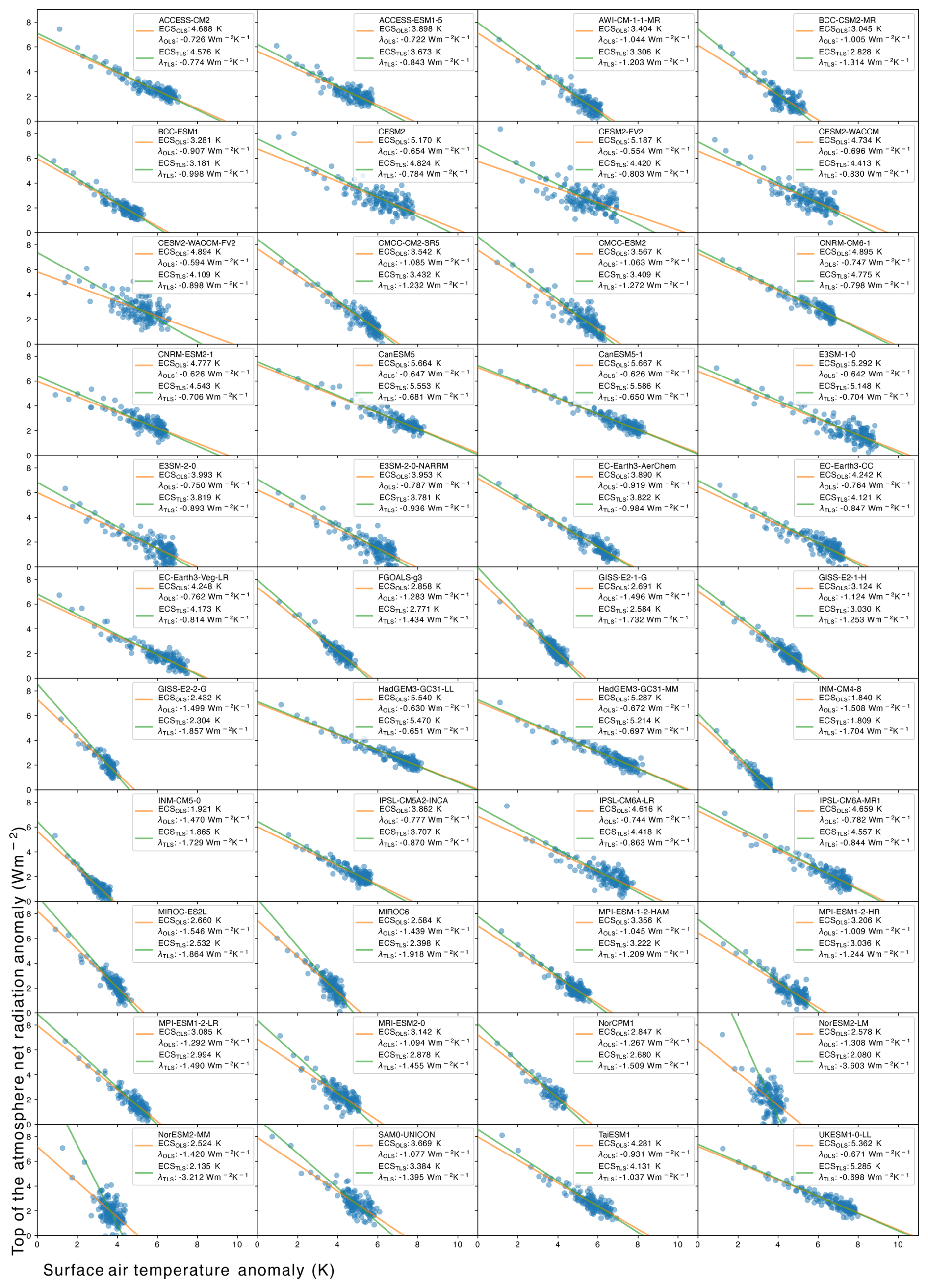
Figure 2 The Gregory plots calculated from the Baseline pathway for each model. The blue scatter plot represents the anomalies over time in the surface air temperature and radiative flux anomaly timeseries. The orange and green lines show linear fits calculated using ordinary and total least squares regression, respectively.

Despite the lack of significance between paths for the ensemble ECS range, we find that the preparation choices matter for a subset of individual models. In the following Sections we discuss the implications of the different choices for each data processing step. This analysis leads to a recommended path for a standardised GM. Note that in the following we use an OLS fit for the ECS estimates unless otherwise specified. For individual ECS estimates across different paths (including a comparison to the Zelinka et al., 2020, calculated values) see Table S2 in the Supplement.

3.1 Global mean weighting

We compare two global mean weighting methods: by grid cell area and cosine of the latitude (Fig. 3a). To ensure a valid comparison, we keep the other data preparation choices constant by following the Baseline pathway: i.e. using rndt as N and the raw piControl for anomalies. Between the two global mean weighting methods, the median [min, max] multi-model ECS range of 3.88 [1.84,5.67] does not change. For most models, the method of global mean weighting has little to no impact. However, we observe four outlier models for which the global mean weighting makes a difference. For AWI-1-1-MR, MPI-ESM-1-2-HAM, and MPI-ESM1-2-HR, weighting the global mean by cos(lat) reduces the ECS estimate by 0.29 K (9 %), 0.36 K (11 %), and 0.21 K (7 %), respectively. For HadGEM3-GC31-MM, weighting by cosine of the latitude increases the ECS estimate by 0.16 K (4 %).

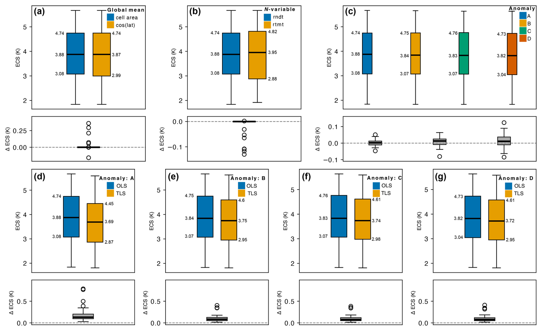
Figure 3 Each subplot shows the inter-model ECS range (upper) and differences between these ranges (lower) comparing the choices at each of the data preparation steps. Boxplots show median first/third interquartile ranges (with ECS labelled in units of K), with whiskers showing the min/max excluding outliers, which are shown as hollow circles. (a) Global mean weighting comparing cell area and cosine of the latitude. (b) N-variable compares the ECS calculated using rndt or rtmt. (c) Anomaly calculation method, with uppercase letters denoting the raw piControl, A, rolling mean, B, linear trend, C, and long-term average, D. (d–g) OLS compared to TLS regression for the four anomaly methods. Note that the differences in range are always calculated as orange subtracted from blue (or green and dark orange subtracted from blue, in the case of plot c). Additionally, note that the difference in ECS range for plots (d–g) share a y axis.

The differences in ECS for global mean weighting methods arise due to each model's grid cell configuration (grid information for each model can be found in Table S1). Each outlier model uses native grid cells that are irregular in shape or size and thus cannot be approximated by cos(lat). Our results suggest that, for these models, it would be an error to use the cos(lat) approximation instead of the native grid cell area variable to calculate the global mean.

In comparison to the two weighting methods we explore, many researchers may use various regridding techniques to calculate the global mean, which we do not consider in this study. Although regridding may be necessary for certain types of studies, we recommend weighting by the model's native grid and using the cell area when calculating the global mean for ECS preparation. This approach eliminates the need to verify if the model's grid is regular and is simpler than the cos(lat) approximation. In cases where cell area data is unavailable, cos(lat) can serve as an approximation, but it may introduce minor errors depending on the model's grid cell configuration. This is a clear demonstration of the importance of the cell area variable in CMIP submissions.

3.2 Net radiative flux variable

To compare the two net radiative flux variables, we again fix the remaining data processing choices as per the Baseline pathway. Of the 44 models in this study, only 35 have the rtmt variable available for both experiments, thus reducing the sample size for this comparison. We note, however, that all 44 models have the required TOA radiation variables meaning they are included for analysing the remaining data processing steps. The median ECS for models using rndt and rtmt, respectively, is 3.88 [1.84,5.67] and 3.96 [1.92,5.67] (Fig. 3b). The choice of N-variable makes no difference for most models, except for, most notably, BCC-CMS2-MR, CESM2, and FGOALS-g3 with an ECS increase of 2 % when using rtmt instead of rndt, BCC-ESM1 and CESM2-FV2 with an ECS increase of 3 %, and INM-CM4-8 with an ECS increase of 6 %.

The differences in ECS between rndt and rtmt are unexpected. A similarity between each of the above models is that they all have a low model top relative to the TOA, however not all models with a low top have a difference in ECS between N variables (for a list of all model tops see Table S3 in the Supplement). From an energy balance perspective, calculating the net radiative flux at different points in the atmosphere is unlikely to result in large changes in flux, given most of the Earth's energy imbalance is taken up by the ocean and land surface, with a common approximation of radiative flux being ocean heat uptake (Forster et al., 2021).

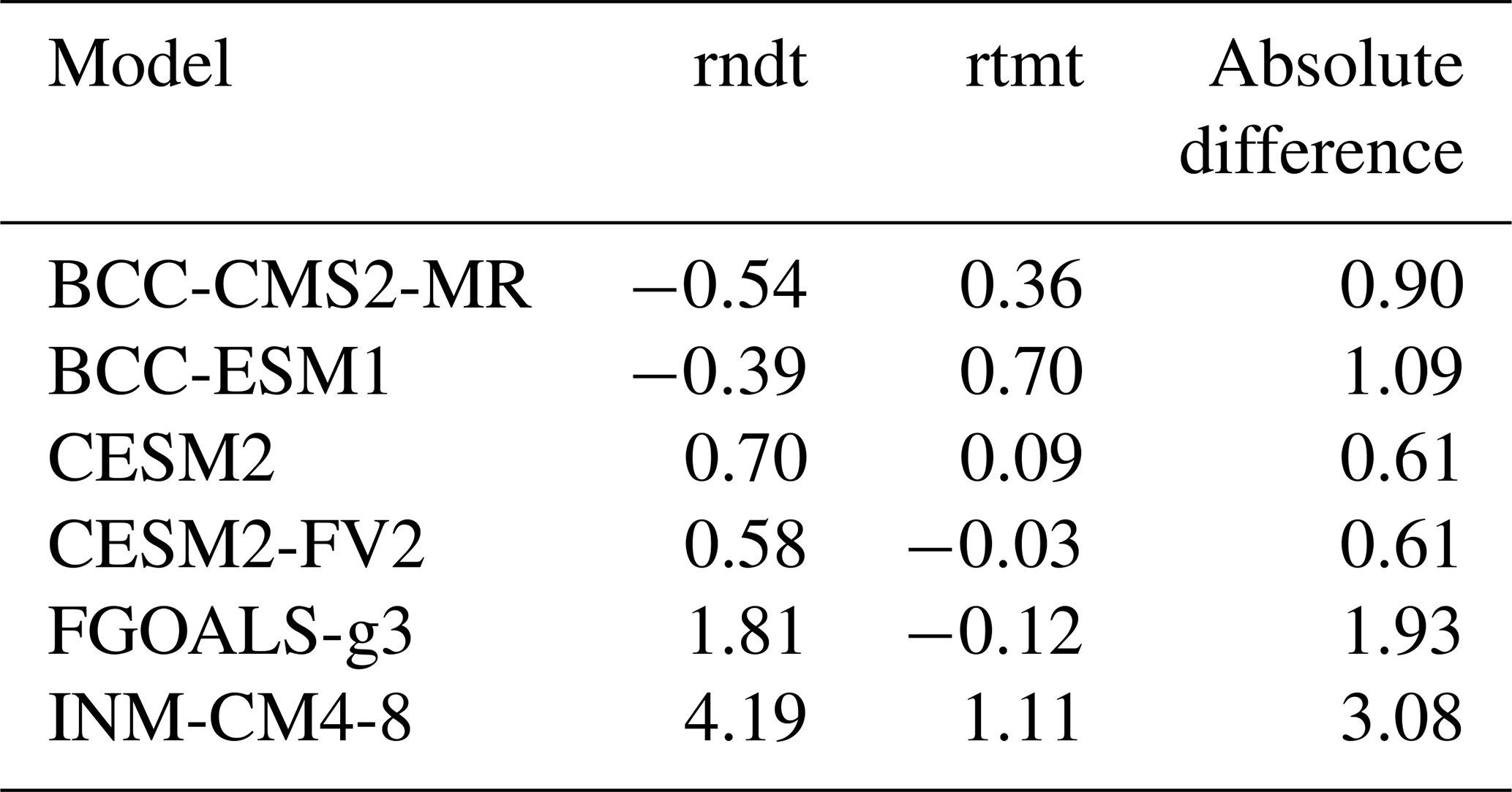
To investigate the differences in rndt and rtmt, we calculate the global annual average over 150 years of the piControl for both variables (see Table S3 for all models). The models with differences in ECS between rndt and rtmt are the only models (apart from SAM0-UNICON) to have notable differences between rndt and rtmt (Table 1), with the largest absolute difference observed for INM-CM4-8 being 3.08 W m⁻². Notably, many models have non-zero differences between rndt and rtmt values – even if these values are equivalent. In theory the piControl should have zero net radiative flux because it is at equilibrium, thus non-zero net radiative flux values are likely a result/indicator of accounting for model drift.

Table 1 Global annual mean N averaged over 150 years of the piControl for rndt, rtmt, and the difference between the two variables (W m⁻²). Only the models with a change in ECS between variables are shown. For the rest of the models see Table S3.

While in theory the ECS should not change between the rndt and rtmt variable, we show that the variables can differ for some models. Given rtmt availability is limited depending on the model, our default suggestion is to use rndt for N.

3.3 Anomaly calculation method

Of the data processing steps analysed in this study, the anomaly calculation method is the most commonly described in the literature. We compare four methods that broadly reflect the different approaches between studies. These approaches form the basis for the labelled paths in Fig. 1: the Baseline, Rolling, Linear, and Long-term paths, which all use the cell area to calculate the global mean, rndt as the N variable, and differ only in their treatment of the piControl for the anomaly calculation.

The multi-model ECS ranges for the Baseline, Rolling, Linear, and Long-term paths are, respectively, 3.88 [1.84,5.67], 3.84 [1.83,5.66], 3.83 [1.83,5.63], and 3.82 [1.83,5.63] (Fig. 3c). To evaluate the impact of the different anomaly methods on individual models, we calculate the differences between the ECS of each model using different anomaly methods. We subtract from the Baseline path the Rolling, Linear, and Long-term paths (Fig. 3c). We observe a wider spread in the differences in ECS between the Baseline and Long-term paths compared to the Rolling and Linear paths. The largest percent difference for individual models is for NorESM2-MM which reduces by 3.4 % (0.09 K) between the Baseline and Long-term paths. In comparison, the largest percent difference between both the Rolling and Linear paths and the Baseline is 1.6 % (0.05 K for MPI-ESM1-2-HR for Linear, and 0.04 K for NorESM2-MM for the Rolling path).

Studies which compute anomalies relative to a smoothed, averaged, or linear piControl cite their methods as aiming to reduce the effects of model drift (Andrews et al., 2012; Armour, 2017; Caldwell et al., 2016; Flynn and Mauritsen, 2020), which refers to a long-term unforced trend in state variables. Since these anomaly methods are replicated and cited by more recent research, we assume that these researchers also aim to reduce model drift (Dong et al., 2020; Eiselt and Graversen, 2022; Po-Chedley et al., 2018; Zelinka et al., 2020).

Unforced experiments, like the piControl, are typically used to diagnose model drift (Gupta et al., 2012, 2013; Irving et al., 2021). However, Hobbs et al. (2016) find that energy biases in CMIP5 models are largely insensitive to the forcing experiment, suggesting that the drift present in the piControl is likely also observed in the abrupt-4xCO₂ experiment. While drift in forced experiments has not been explicitly examined for the CMIP6 ensemble, Irving et al. (2021) assume it to be equivalent to that in the piControl, based on the findings of Hobbs et al. (2016) for CMIP5. Thus, assuming an equivalent drift is present in both the abrupt-4xCO₂ and piControl experiments, we would expect that the Baseline, Rolling, and Linear paths implicitly removes model drift following the subtraction. Calculating the anomaly relative to the piControl long-term average, however, does not account for biases that may be introduced by model drift.

In addition to model drift, the correlation between N and ΔT is another approach of comparing the anomaly calculation methods. The median absolute correlations across all models for the Baseline, Rolling, Linear, and Long-term paths are respectively 0.88 [0.57,0.95], 0.93 [0.64,0.97], 0.93 [0.65,0.98], and 0.93 [0.65,0.98]. The differences in correlation likely results from a reduction in variance for the Rolling, Linear, and Long-term paths in comparison to the Baseline. For ΔT, the variance is less sensitive to the anomaly calculation method, with median variances across all models being 0.77, 0.76, and 0.73, and 0.70 for the Baseline, Rolling, Linear, and Long-term paths, respectively. However, for N, the median variances show a more substantial difference: 0.81, 0.70, 0.71, and 0.70 for each respective path.

While the differences in correlation and variance between anomaly methods have minimal impact on the ECS estimates for an OLS fit, we observe more notable differences when comparing an OLS and TLS fit (Fig. 3d–g). The median differences between OLS and TLS for the Baseline, Rolling, Linear, and Long-term paths are 0.13 K [0.03,0.79], 0.08 K [0.02,0.4], 0.08 [0.02,0.39], and 0.08 K [0.02,0.41], respectively. Applying a trend or climatology to the piControl prior to the anomaly calculation reduces scatter between variables, thus increasing the absolute correlation compared to the Baseline pathway.

Based on our anomaly method analysis we recommend that future climate sensitivity studies apply either a rolling average or linear trend to the piControl. We favour these two methods due to their implicit treatment of model drift (in comparison to the long-term average method), and due to their larger absolute correlation and avoided artificially inflated variance (in comparison to the raw piControl method) which provides improved alignment with the assumptions that underpin the linear regression. We note here that choices in drift correction method may have a larger impact on anomalies calculated over historical simulations relative to abrupt-4xCO₂ experiments, which may warrant further study. When choosing more specifically between the rolling average and the linear trend method, we recommend the 21 year rolling average. This method has been used to compare both CMIP5 and CMIP6 model ensembles (Caldwell et al., 2016; Zelinka et al., 2020), providing consistency with existing literature.

3.4 Linear regression method

In this study, we consider two linear regression fits: ordinary and total least squares regression. To the best of our knowledge, most researchers use the OLS fit of N against ΔT to calculate the slope (λ) and ECS when using the Gregory method, e.g. (Andrews et al., 2012, 2015; Armour, 2017; Bloch-Johnson et al., 2021; Caldwell et al., 2016; Chao and Dessler, 2021; Dai et al., 2020; Dong et al., 2020; Rugenstein and Armour, 2021; Zelinka et al., 2020; Zhou et al., 2021). This is consistent with the original approach of Gregory et al. (2004), who treated temperature as the “arbitrary” choice of independent variable. However, across CMIP6 models, this choice is not arbitrary given the median slope (λ) across models is affected by the choice of independent variable; 0.88 $\mathrm{W}{\mathrm{m}}^{-\mathrm{2}}{\mathrm{K}}^{-\mathrm{1}}$ when using ΔT and 0.74 $\mathrm{W}{\mathrm{m}}^{-\mathrm{2}}{\mathrm{K}}^{-\mathrm{1}}$ when using N (Fig. 4a). For individual models, the dependent variable of choice may result in even more substantial variation (Fig. 4b), notably impacting the derived climate sensitivity.

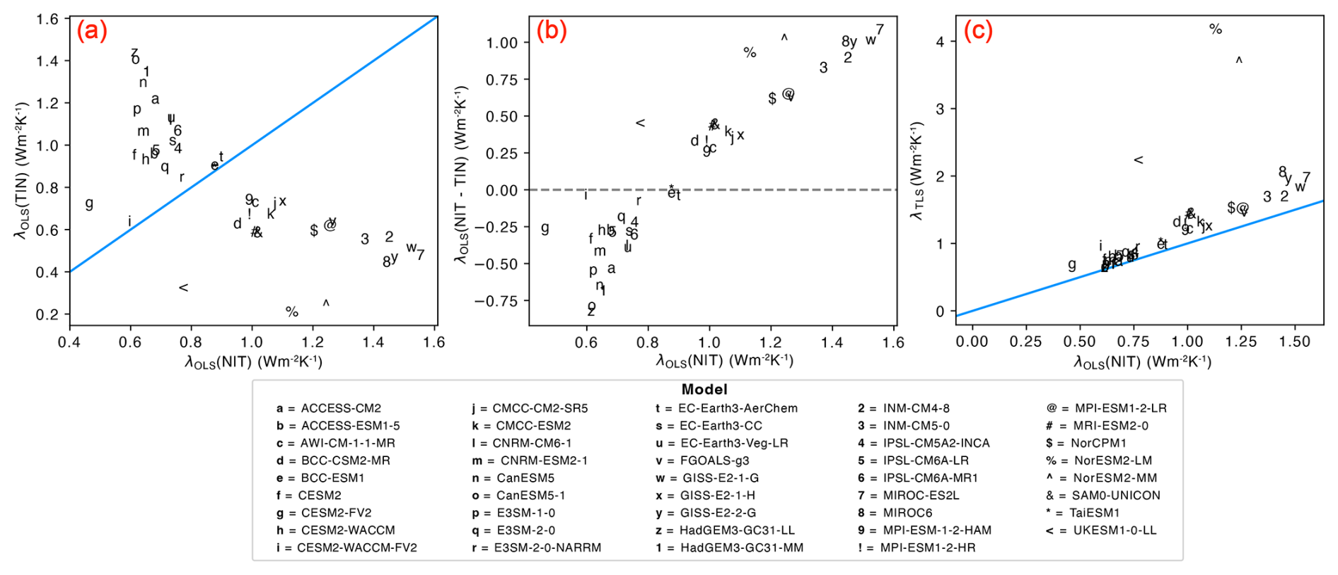
Figure 4 (a) The slope (λ) of each CMIP6 model calculated using ordinary least squares (OLS) regression with ΔT as the independent variable (x axis) and N as the independent variable (y axis). Blue line shows the linear relationship required for the choice of independent variable to make no difference. (b) y axis showing the difference in slope for each CMIP6 model between the OLS regression based on ΔT or N as the independent variable. x axis is the same as (a). Dashed line at y=0. (c) The slope of the linear regression fit for each model calculated using total least squares (TLS) on the y axis and OLS on the x axis. Note that (a) and (b) follow the same form as Appendix C of Gregory et al. (2020), but use abrupt-4xCO₂ experiment here instead of the historical simulation. Each axis has units of $\mathrm{W}{\mathrm{m}}^{-\mathrm{2}}{\mathrm{K}}^{-\mathrm{1}}$.

For OLS to provide a reasonable fit, the data must meet two key conditions: there should be a clear dependent variable, and the independent variable must be measured without error (Isobe et al., 1990). In contrast, TLS accounts for errors in both variables, treats them symmetrically, and is more appropriate when seeking to determine a relationship between variables rather than establishing a causal link. Here, errors are not measurement errors, but instead are the random variations on top of the signal we are trying to fit. So, while it is not strictly an error, natural variability plays basically the same role as an error in this study.

Gregory et al. (2004) justify using OLS over alternate regression methods on the basis of the minimal “scatter about a straight line resulting from internally generated variability”. They find that the minimal scatter in the data leads to a negligible difference in slope regardless of the choice of dependent variable. However, this rationale was based on a single abrupt-4xCO₂ experiment from the HadSM3 slab ocean model. In comparison, we observe substantial scatter across a range of CMIP6 models (Fig. 2), indicating that the original assumption of minimal scatter does not hold for the more complex fully coupled ESMs developed since 2004. This suggests that the original justification of OLS is worth reconsidering.

Previous research has justified using temperature as the independent variable. Murphy et al. (2009) found that, on short timescales, temperature variations drive changes in outgoing radiation. Similarly, Forster and Gregory (2006) observed that temperature generally leads radiative flux, and Gregory et al. (2020) followed the physical intuition that temperature determines the magnitude of radiative flux. However, these justifications are primarily grounded in observations. For idealised model simulations, the leading relationship between radiative flux and temperature is not always evident from the timeseries alone. This is particularly true for the strongly perturbed abrupt-4xCO₂ experiments, where the climate system is responding to an imposed radiative forcing that is far more extreme than anything observable in the real world, making it difficult to identify a relationship with N lagging ΔT.

Given the absence of a clear causal direction from which to define an independent variable, we turn to the second key assumption of OLS: the identification of error. If one variable exhibits errors that are uncorrelated with the other variable, we typically assign the former as the dependent variable, assuming the independent variable is perfectly known (see Appendix B in Gregory et al., 2020). However, if both variables contain uncorrelated errors, TLS provides a more appropriate regression approach, as it accounts for errors in both variables rather than treating one as exact.

Unlike in observational timeseries, where errors are often well-characterised – such as instrumental uncertainty or random measurement errors – errors in climate models primarily arise from unforced variability (Gregory et al., 2020). This variability functions similarly to noise in a statistical sense, obscuring the signal we aim to extract. While it does not introduce randomness in the same way as observational errors, it complicates regression analysis by adding fluctuations that are unrelated to the primary forcing-response relationship of interest.

We can avoid inflating the variability in the ΔT and N timeseries through the anomaly calculation method. The methods which apply a rolling mean or linear fit to the piControl experiment are suitable, for example. Otherwise, subtracting raw piControl runs would inflate the variability and decrease the absolute correlation between the two variables. However, to our knowledge no method exists which removes all natural variation from the model while leaving the pure forced signal. Gregory et al. (2020) used the historical ensemble mean (simulations of the recent past from approximately 1850 to 2014, Eyring et al., 2016) of multiple members of MPI-ESM1.1 to argue that temperature exhibits minimal noise, supporting its use as the independent variable. However, they also acknowledge that this assumption may not hold for other ESMs. Given we cannot confidently justify treating either N or ΔT as the perfect independent variable, OLS may not be the most robust regression method in this context.

While we find that statistical arguments favour TLS, a number of arguments exist for retaining OLS as the preferred regression method. Firstly, retaining OLS is consistent with the last two decades of ECS research, allowing for comparisons between and within CMIP generations (although recalculating using new methods is an option given the long-term archive and access to data provided by the Earth System Grid Federation). Secondly, physical reasoning regarding ECS bias supports OLS. The climate sensitivity estimated as the ΔT-intercept from the GM is biased relative to the true ECS values obtained from fully coupled simulations run for multiple millennia of simulation years (Rugenstein et al., 2020). We find that TLS systematically yields lower ECS values compared to OLS (Fig. 4c). Comparing an OLS and TLS fit, the median ECS reduces from 3.9 to 3.7 K, with the percentage difference for individual models ranging from 1.4 % (0.08 K) for HadGEM3-GC31-LL to 24 % (0.65 K) for NorESM2-LM. The reduction between linear fits is consistent with findings of Forster and Gregory (2006), who deliberately chose the regression method which gave the largest sensitivity estimate. The low bias of TLS likely arises given TLS weights the earlier years of the regression more heavily compared to OLS. While TLS may introduce a low bias in ECS estimates, it is worth noting that this method could potentially reduce the low bias in effective radiative forcing (ERF) observed in studies that calculate ERF using OLS over the full 150 year simulation period (Forster et al., 2016; He et al., 2025; Lutsko et al., 2022; Smith et al., 2020).

Clearly, the choice of regression matters. While we analyse and compare OLS and TLS fits, exploring additional regression methods, such as the York method, or Deming regression, may provide further insights (Him and Pendergrass, 2024; Lewis and Curry, 2018; Wu and Yu, 2018). We recommend that future ECS studies clearly report the regression method used and we encourage future research into more robust regression methods. Despite this, in the absence of clearer evidence, we believe that OLS should remain the basis of comparison to remain consistent with the majority of the literature.

3.5 Uncertainty range for individual ECS estimates

Calculating uncertainty over ECS estimates is an important step that is lacking from most of the climate sensitivity studies we cite in this paper. In the original study, Gregory et al. (2004) calculate uncertainty as the root mean square deviation from the OLS regression fit. More recent studies that calculate an uncertainty range typically use a standard bootstrap approach, randomly sampling data points from the time series (with replacement) to generate 10 000 subsets for performing the Gregory regression (Andrews et al., 2012; Bloch-Johnson et al., 2021; Rugenstein et al., 2020). This is a common approach for constructing an uncertainty range; however, it assumes annual independence of data, which does not hold for some models (identified in the following discussion).

To assess the level of inter-annual dependence across models, we calculate the autocorrelation function of the ΔT timeseries following the removal of a quadratic fit for the four different anomaly method pathways (Fig. S2 in the Supplement). The autocorrelation function plots the correlation between a time series and its lagged versions, with particular focus on the correlation between adjacent timepoints. This analysis reveals two common temporal relationships exhibited by the models: an exponential decaying decorrelation, where the relationship between years decreases as more time passes, and an oscillating relationship, indicating that a periodic cycle is influencing the climate system.

While most models exhibit the exponential decaying decorrelation, the models which show an oscillating behaviour include CMCC-CM2-SR5, CMCC-ESM2, EC-Earth3-AerChem, EC-Earth3-Veg, EC-Earth3-Veg-LR, GISS-E2-1-G, GISS-E2-1-H, MIROC6, NorESM2-MM, UKESM1-0-LL which have periods of between 3-6 years. For some of these models the process displayed depends on the anomaly calculation method, for example CMCC-CM2-SR5 shows an oscillating process for anomaly methods (B), (C) and (D), whereas when using the raw piControl for anomalies it shows an exponentially decaying process.

The oscillating behaviour within these models is an unlikely feature of independent samples, suggesting the presence of an inter-annual or -decadal mode of variability. For example, a four-year period could be indicative of the El Niño Southern Oscillation (ENSO), however in the real world ENSO has an irregular period of between 2 to 7 years (Tang et al., 2018). Thus, a model with such a consistent four year ENSO – or other mode of variability – signal would be an unrealistic representation of the real world and should be considered when using the model for climate sensitivity analysis and calculating the uncertainty range. We note that this is not necessarily a feature of the anomaly calculation, however, and instead is an underlying feature of the model given the residuals of the raw abrupt-4xCO₂ time series also exhibit similar periodic behaviour for the same models (Fig. S3 in the Supplement).

It is important to consider how interannual dependence affects the confidence of ECS estimates. Gregory et al. (2004) acknowledge that interannual variability can have an impact on calculating the uncertainty range, but argue that ignoring the time dependence of the time series primarily results in a narrower uncertainty range rather than introducing bias. Jain et al. (2021) also highlight that ΔT and N timeseries exhibit temporal dependence, leading to an underestimation of errors. They address this by either adjusting the number of model years using an effective sample size based on time-lag correlations or by applying a standard bootstrap resampling approach, as done by Andrews et al. (2012). However, these approaches may result in different uncertainty ranges, given the standard bootstrap approach assumes independent data points, which is not true for all models.

We find that the interannual time dependence of the data varies by model and anomaly calculation method. To account for this, we compare two bootstrap approaches: a standard bootstrap, replicating previous studies, and a block bootstrap with a block size of four years, which accounts for interannual correlations. We calculate a 95 % confidence interval using the two bootstrap approaches around the ECS estimate for individual models (Fig. 5a; see Table S4 in the Supplement for the confidence intervals calculated for each model using both bootstrap approaches). For simplicity, we use the Baseline pathway and the OLS fit (although we also show the same figure in supplementary, calculated using a TLS fit, Fig. S4 in the Supplement).

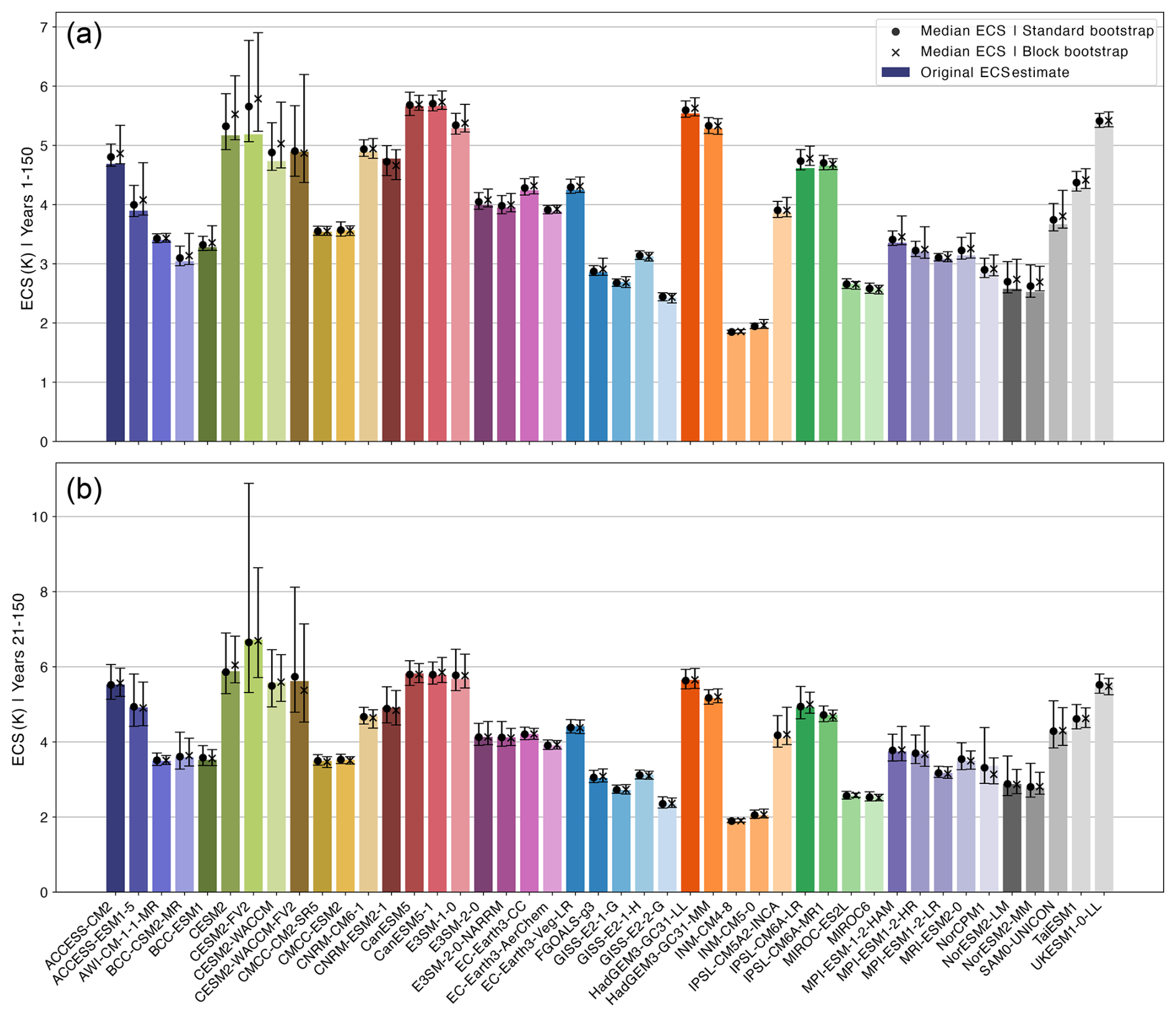
Figure 5 ECS uncertainty using an ordinary least squares fit. (a) ECS estimates for each model using the Baseline Gregory Method, using years 1–150. Bars represent 95 % confidence intervals, with medians calculated using a simple bootstrap (solid circle) and a moving block bootstrap with a block size of 4 (cross). (b) The same as (a), but the ECS and bootstrap uncertainties are calculated using years 21–150 of the N and ΔT anomaly timeseries. See Methods for details on confidence interval calculations.

For most models the median ECS calculated using both the bootstrap approaches are larger than the original ECS estimate – for 40 models using the standard bootstrap, and 37 models using the block bootstrap. Additionally, for 27 models the median ECS calculated using the block bootstrap is larger than the median ECS calculated from the standard bootstrap. Most notably, however, we find that the uncertainty range for some models sits well above the original ECS estimate (e.g. ACCESS-CM2, ACCESS-ESM1-5, CESM2-FV2, and CESM2-WACCM, NorESM2-LM, NorESM2-MM, TaiESM1).

Clearly, the uncertainty ranges for individual models have a high bias, regardless of the bootstrap approach. This bias arises from a sensitivity to the early years of the experiment. The Gregory plots (Fig. 2) for these models show data points with low temperature anomalies and high radiative flux anomalies in the initial years. When bootstrapping across all 150 years, these early data points are often underrepresented in resampled datasets, leading to a systematic overestimation of the ECS compared to the original calculation. However, this reasoning could support the previous research which excludes early years from the data to calculate the ECS (Andrews et al., 2015; Dunne et al., 2020). Rather than overestimating the ECS, the uncertainty ranges may better represent the “true” value for an equilibrium climate.

To eliminate the differences between the bootstrap uncertainty and the original ECS estimate, we repeat the analysis while restricting both the original ECS calculation and bootstrap uncertainty estimation to years 21–150 (thus replicating the method of Bloch-Johnson et al., 2021). This removes the early-year influence, yielding more consistent confidence intervals (Fig. 5b). We note that excluding the first 20 years has implications for radiative forcing estimates, as it raises the question of how long a model must run before the climate response stabilises. While this warrants further investigation, we leave this for future research, as our study focuses specifically on ECS estimation.

Despite the benefit of using years 21–150 on the confidence interval calculations, additional factors must be considered. Excluding early years from the regression is a common alteration to the GM (Andrews et al., 2015; Armour, 2017; Bloch-Johnson et al., 2021; Dai et al., 2020; Dunne et al., 2020; Lewis and Curry, 2018). However, the exclusion of the first 20 years results in a reduced absolute correlation between N and ΔT. For years 1–150 and 21–150, respectively, the median absolute correlation is 0.85 [0.49,0.94] and 0.63 [0.3,0.86]. The reduction in absolute correlation is most important when considering the choice of linear regression fit, given the difference between the inter-model ECS distribution using OLS and TLS is larger when using years 21–150 compared to years 1–150.

For future research, it is important for studies to include an ECS uncertainty range around the estimate. Ideally, modelling groups would provide multiple simulations of the abrupt-4xCO₂ timeseries to provide a more robust basis for the uncertainty assessment, given this would allow for resampling from independent experiments. However, given this is unlikely across all modelling groups, we recommend plotting the autocorrelations of the ΔT and N anomaly time series to assess interannual dependence in the data to inform the bootstrap resampling method. Additionally, alternative uncertainty calculation methods could be investigated which downweight the early years of the experiments, although this may be less necessary if CMIP7 abrupt-4xCO₂ experiments are run to 300 simulation years instead of the previously required 150 years (Dunne et al., 2025).

4 Discussion and conclusions

For each of the 44 CMIP6 models in this study, we compare 32 ECS estimates derived from alternative choices in data preparation steps and linear regression methods. We find no statistically significant difference between the inter-model ECS ranges across the data preparation paths, or when comparing ordinary and total least squares regression fits. Literature which compares the ECS inter-model spread across CMIP6 models, e.g. (Chao and Dessler, 2021; Dong et al., 2020; Eiselt and Graversen, 2023; Flynn and Mauritsen, 2020; Meehl et al., 2020; Rugenstein et al., 2020; Zelinka et al., 2020), are unlikely to see a meaningful difference in results by recalculating based on an alternate data preparation pathway.

Differences in ECS estimates arise, however, when comparing a subset of CMIP6 models. At each step, the largest individual model ECS differences are 11 % for global mean weighting, 6 % for N-variable, 3 % for anomaly method, and 24 % for linear regression method. Additionally, whilst individual anomaly methods do not alter the ECS much for just the OLS fit, the range is narrower for anomaly methods which use a rolling climatology or linear trend applied to the piControl, resolving some of the differences between OLS and TLS, likely due to the increase in absolute correlation compared to the raw piControl.

OLS has traditionally been the default linear regression fit for the Gregory Method. However, we recommend further exploration of alternative approaches – such as TLS – to better balance physical understanding with statistical robustness in ECS estimation. We find that, for most models, the choice of dependent variable influences the slope of the regression, contradicting previous assumptions that the choice is arbitrary (Andrews et al., 2015; Gregory et al., 2004). Additionally, given errors – or interannual variations on top of the forced signal – are present in both variables, we do not confidently identify one variable over the other as being simulated without error. For consistency with previous research and given the physical reasoning of GM-calculated ECS low bias, OLS should remain the standard, but with room for further investigation.

Two additional aspects of ECS estimation which we do not investigate in this study are: the choice of CO₂ perturbation experiment, and using different time periods for the regression. Despite the ECS metric being defined as the response to CO₂ doubling, research typically uses CO₂ quadrupling to maximise the signal-to-noise ratio (Bryan et al., 1988; Dai et al., 2020; Washington and Meehl, 1983). However, a large body of literature identifies a non-linear scaling for each consecutive CO₂ doubling (Bloch-Johnson et al., 2021; Chalmers et al., 2022; Hansen et al., 2005; Li et al., 2013; Meraner et al., 2013; Mitevski et al., 2021, 2022, 2023; Russell et al., 2013). This could overestimate the ECS relative to an abrupt-2xCO₂ experiment. However, research also shows that the Gregory method can underestimate the true ECS by 17 % (Rugenstein et al., 2020), 14 % (Dunne et al., 2020), or 10 % (Li et al., 2013). Sherwood et al. (2020) propose that this underestimation, combined with the overestimation due to the nonlinear climate response to consecutive CO₂ doublings, could potentially “cancel out”, resulting in an accurate sensitivity estimate using the Gregory method. However, this hypothesis has not been systematically assessed in the literature and warrants further investigation.

The landscape of ECS estimation is set to change for CMIP7, following the recommendation for modelling groups to extend the abrupt-4xCO₂ experiment requirements from 150 to 300 simulation years (Dunne et al., 2025). This extended simulation is expected to narrow the gap between GM-estimated ECS and the results from ESMs run to near-equilibrium (Dunne et al., 2020; Rugenstein et al., 2020). A longer simulation will likely increase the ECS when calculated over the full 1–300 years, potentially affecting comparability to previous CMIP generations. Given these changes, we recommend that future studies applying the GM to CMIP7 data calculate the ECS based on both 1–150 and 1–300 years. Computing these two values will allow comparison to CMIP5 and CMIP6, provide further evidence of inconstant feedbacks (Rugenstein et al., 2020), and allow the research community to evaluate more thoroughly the merits and limitations of the linear relationship currently used for ESC estimation.

Table 2 The steps, choices, recommendations, and caveats we investigate in this study. These recommendations should form the basis of a standardised Gregory method for future research.

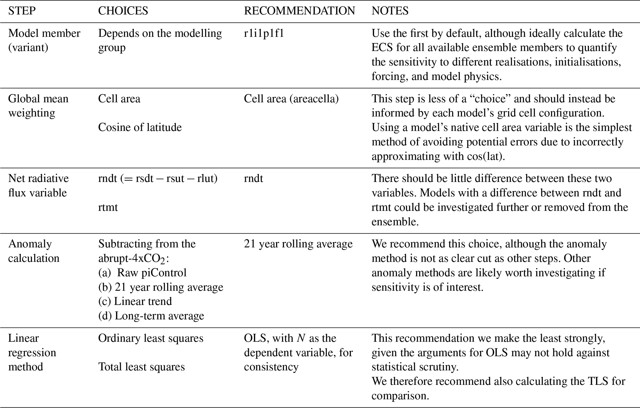
Based on our findings, we provide recommendations for standardising the GM (Table 2) and a checklist of what to include in future climate sensitivity research. Our standardisation framework details the steps involved, the alternative steps we investigate, our proposed recommendations, and associated caveats. We acknowledge that not all studies applying the Gregory method have the ECS as their primary focus, and researchers may make alternative choices for their analyses that we have not explored. We therefore include a checklist to ensure that, at minimum, future studies clearly report their methods, choices, and order of operations to support transparency and reproducibility (with, in our opinion, the simplest option being to simply publish code alongside studies, as this is the least ambiguous description of what was actually done). With the upcoming release of CMIP7 models, data preparation choices may play a more critical role than for CMIP6, underscoring the need for a standardised Gregory method calculation.

Checklist:

□

Provide public access to all code used in the analysis

□

Clearly describe all data preparation steps in the methods section, including:

• All variables used

• Any differences from the recommended standardisation

• Order of operations

□

Verify each model's grid configuration (to inform global mean weighting method)

□

Calculate the ECS based on both an OLS and TLS regression

□

For CMIP7, calculate the ECS based on both years 1–150 and 1–300

□

Calculate uncertainty around individual ECS estimates