Predicting and correcting the influence of boundary conditions in regional inverse analyses

Regional inverse analyses of atmospheric trace gas observations quantify gridded two-dimensional surface fluxes by fitting the observations to simulated concentrations from a transport model, usually by Bayesian optimization regularized by a gridded prior flux estimate. Regional inversions rely on the specification of background concentrations given by the boundary conditions (BCs) at the edges of the inversion domain, but biases in the BCs propagate to biases in the optimized fluxes. We develop a theoretical framework to explain how errors in the BCs influence the optimized fluxes as a function of the prior and observing system error statistics and of model transport. We derive a preview metric to estimate the BC-induced errors before conducting an inversion to support domain specification and a diagnostic metric to accurately quantify these errors after solving the inversion. We compare two methods to correct BC biases as part of an inversion, either directly by optimizing BC concentrations (boundary method) or indirectly by expanding the domain and correcting grid cell fluxes outside the region of interest (buffer method). We demonstrate that the boundary method is generally more accurate, physically grounded, and computationally tractable.

1 Introduction

Regional inversions of observed atmospheric concentrations of long-lived trace gases quantify surface fluxes by fitting simulated concentrations from a transport model to the observations assuming boundary conditions (BCs) at the edge of the inversion domain. Such analyses can improve knowledge of fluxes and their trends on local to continental scales at high spatiotemporal resolution while avoiding the need to accurately quantify fluxes and concentrations globally (Sargent et al., 2021; Nesser et al., 2024; Byrne et al., 2024). However, BCs are often uncertain and biases in the BCs propagate to the inferred fluxes. Here we examine the problem of how BC biases affect regional inversions of greenhouse gas fluxes and develop a framework to predict and correct the influence of these biases.

BCs can be provided by coarse-resolution global simulations (Göckede et al., 2010; Wecht et al., 2014), by statistical or meteorological analysis of trace gas observations (Lauvaux et al., 2016; Balashov et al., 2020), or by combining simulated and observed concentrations (Sargent et al., 2018; Estrada et al., 2025). The information used to constrain BCs is often spatiotemporally sparse and may be biased. Even small BC biases can cause large biases in the inferred fluxes (Göckede et al., 2010; Lauvaux et al., 2012; Karion et al., 2021). BC biases are particularly critical for regional inverse analyses of long-lived gases such as carbon dioxide and methane where concentrations and variability can depend significantly on inflow.

Regional inversions generally infer gridded surface fluxes (the state vector) by minimizing a Bayesian cost function that accounts for the error statistics of the observing system (including the observations and transport model) and of the prior flux estimate used to regularize the solution. BC biases may be corrected as part of the inversion by optimizing BC concentrations as part of the state vector (Lauvaux et al., 2012; Wecht et al., 2014), by allowing buffer grid cells at the edge of the domain to absorb BC biases (Shen et al., 2021; Varon et al., 2022), or by combining these approaches (Estrada et al., 2025).

We present here a theoretical framework to predict, diagnose, and correct the influence of BC biases on the posterior gridded surface fluxes generated by a regional inversion (Sect. 2). We consider an inert trace gas with no sources or sinks within the inversion domain other than the surface fluxes. We demonstrate this framework with increasingly complex one- and two-dimensional simulation experiments that invert pseudo-observations of a long-lived trace gas generated using known fluxes and BCs (Sects. 3 and 4, respectively). Throughout, we compare different methods to correct BC biases within inversions and present metrics that estimate the effect of BC biases.

2 Analytical solution for the effect of boundary condition errors

We describe the analytical inverse solution, which we use to derive an exact solution (diagnostic) for the sensitivity of the posterior fluxes to a BC bias (Sect. 2.1). We apply this diagnostic to a simple one-dimensional transport model to determine how these errors depend on constant inversion parameters (Sect. 2.2). We then generalize the results using a two-box model applicable to two-dimensional inversions with variable inversion parameters. We use this two-box model to derive a preview metric that predicts the sensitivity of posterior fluxes to BC biases for a given inversion configuration, allowing the user to improve inversion parameters as needed before solving the inversion (Sect. 2.3).

2.1 Diagnostic equation

Given an n-dimensional state vector of gridded fluxes x and an m-dimensional vector of observations y, both with normally distributed errors, the optimal flux estimate $\widehat{\mathit{x}}$ is obtained by minimizing a Bayesian cost function

$$\begin{array}{}\text{(1)}& \begin{array}{rl}{\displaystyle }J\left(\mathit{x}\right)=& {\displaystyle }(\mathit{x}-{\mathit{x}}_{\mathrm{A}}{)}^{\mathrm{T}}{\mathbf{S}}_{\mathrm{A}}^{-\mathrm{1}}(\mathit{x}-{\mathit{x}}_{\mathrm{A}})\\ {\displaystyle }& {\displaystyle }+(\mathit{y}-F(\mathit{x}\left){)}^{\mathrm{T}}{\mathbf{S}}_{\mathrm{O}}^{-\mathrm{1}}\right(\mathit{y}-F\left(\mathit{x}\right)),\end{array}\end{array}$$

where x_A and S_A are the prior flux estimate and error covariance matrix, respectively, S_O is the observing system error covariance matrix representing uncertainties in the observations and the transport model, and F is the transport model (Brasseur and Jacob, 2017). We assume as is standard that the transport model initial conditions are given by a sufficiently long spin-up simulation driven by the BCs so that the initial conditions are consistent with the BCs. If the transport model is linear, then $F\left(\mathit{x}\right)=\mathbf{K}\mathit{x}+\mathit{c}$ where $\mathbf{K}=\partial F/\partial \mathit{x}$ is the Jacobian matrix. The vector c represents the model background defined by the transport of the BCs to the same spatiotemporal locations as the observations. If the BC concentrations are optimized as part of the inversion, information about the background is instead contained in the state vector and in the columns of the Jacobian matrix so that c=0.

We can write the analytical solution for the cost function minimum that yields the optimal (posterior) flux estimate $\widehat{\mathit{x}}$ as

$$\begin{array}{}\text{(2)}& \widehat{\mathit{x}}={\mathit{x}}_{\mathrm{A}}+\mathbf{G}(\mathit{y}-(\mathbf{K}{\mathit{x}}_{\mathrm{A}}+\mathit{c}\left)\right)\end{array}$$

where

$$\begin{array}{}\text{(3)}& \mathbf{G}={\displaystyle \frac{\partial \widehat{\mathit{x}}}{\partial \mathit{y}}}={\left({\mathbf{K}}^{\mathrm{T}}{\mathbf{S}}_{\mathrm{O}}^{-\mathrm{1}}\mathbf{K}+{\mathbf{S}}_{\mathrm{A}}^{-\mathrm{1}}\right)}^{-\mathrm{1}}{\mathbf{K}}^{\mathrm{T}}{\mathbf{S}}_{\mathrm{O}}^{-\mathrm{1}}\end{array}$$

is the gain matrix that represents the sensitivity of the posterior fluxes to the observations. We can separate the model-observation difference into the contributions from the errors in the prior fluxes relative to the true fluxes (x_T) and the errors in the observing system $(\mathit{\epsilon }=\mathit{y}-(\mathbf{K}{\mathit{x}}_{\mathrm{T}}+\mathit{c}\left)\right)$ so that

$$\begin{array}{}\text{(4)}& \widehat{\mathit{x}}={\mathit{x}}_{\mathrm{A}}+\mathbf{A}({\mathit{x}}_{\mathrm{T}}-{\mathit{x}}_{\mathrm{A}})+\mathbf{G}\mathit{\epsilon }\end{array}$$

where $\mathbf{A}=\partial \widehat{\mathit{x}}/\partial \mathit{x}=\mathbf{GK}$ is the averaging kernel matrix, a measure of inversion information content that gives the sensitivity of the posterior fluxes to the true fluxes. The trace of the averaging kernel matrix gives the degrees of freedom for signal (DOFS), the number of independent pieces of information quantified by the inversion (Rodgers, 2000).

The posterior error induced by a BC error (ε_C) is derived by comparing the posterior fluxes produced with the true BC (c_T) to an inversion with the BC error ($\mathit{c}={\mathit{c}}_{\mathrm{T}}+{\mathit{\epsilon }}_{\mathrm{C}}$):

$$\begin{array}{}\text{(5)}& \mathrm{\Delta }\widehat{\mathit{x}}=-\mathbf{G}{\mathit{\epsilon }}_{\mathrm{C}}.\end{array}$$

We define Eq. (5) as the diagnostic that estimates the effect of BC bias on the posterior fluxes given an explicitly constructed Jacobian matrix and assumed BC error statistics, which can be estimated from observed variability of background concentrations. BC-induced posterior errors are controlled by the gain matrix, which is a function of the observing system errors, prior flux errors, and transport as represented by the Jacobian matrix.

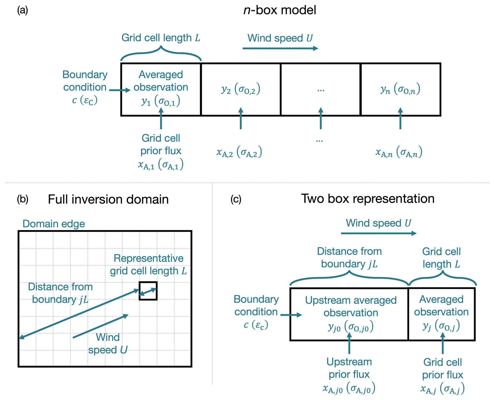
Figure 1 One-dimensional and two-box models of a passive trace gas to quantify the influence of BCs on inverse analyses. The one-dimensional model (a) simulates the concentrations of an inert trace gas over n grid cells of length L given a prescribed BC c, fluxes $x=[x_{\mathrm{1}},x_{\mathrm{2}},\mathrm{\dots },x_n{]}^{\mathrm{T}}$, and advection with wind speed U. The two-box model (c) generalizes an inverse analysis optimizing fluxes over a two-dimensional grid (b) where all grid cells have a representative grid cell length L given the wind direction. Each grid cell in the domain is reduced to a two-box model composed of a cluster of the j upwind grid cells (index j0) and the grid cell itself (index j). In all models, the inversion is solved with the averaged observation y_i over each grid cell $i=\mathit{\{}\mathrm{1},\mathrm{\dots },n\mathit{\}}$ with corresponding error standard deviation σ_O,i. The inversion is regularized by the prior flux x_A,i in each grid cell with corresponding prior error standard deviation σ_A,i.

2.2 One-dimensional model

To better understand how observing system errors, prior flux errors, and transport determine the influence of BC biases on posterior flux estimates (Eq. 5), we consider a one-dimensional horizontal transport model with constant wind speed U. Figure 1a depicts this model for n grid cells of length L. The Jacobian matrix for this transport model is derived through steady-state mass balance (Sect. S1 in the Supplement) to be lower diagonal with constant values given by

$$\begin{array}{}\text{(6)}& \mathit{\tau }=\mathit{\alpha }{\mathit{\tau }}^{\prime }\end{array}$$

where α converts between the flux units and the observation units and τ^′ is the grid cell residence time calculated as ${\mathit{\tau }}^{\prime }=L/U$. The trace gas sources in the model are the BC c and fluxes $\mathit{x}=[x_{\mathrm{1}},x_{\mathrm{2}},\mathrm{\dots },x_n{]}^{\mathrm{T}}$. We assume that the m observations are uniformly distributed in space and time with constant uncorrelated error variance ${\mathit{\sigma }}_{\mathrm{O}}^{\mathrm{2}}$. We solve the inversion (Eq. 2) using the averaged observations in each grid cell so that the observing system error covariance matrix S_O is diagonal with constant error variances ${\mathit{\sigma }}_{\mathrm{O}}^{\mathrm{2}}/m_{\mathrm{g}}$ where $m_{\mathrm{g}}=m/n$ is the number of observations in each grid cell. We assume constant prior fluxes x_A and diagonal prior error covariance matrix S_A with constant error variances ${\mathit{\sigma }}_{\mathrm{A}}^{\mathrm{2}}$. We define the dimensionless, domain-average information ratio R of the prior error variances in concentration units to the observing system error variances

$$\begin{array}{}\text{(7)}& R=m_{\mathrm{g}}{\left({\displaystyle \frac{\mathit{\tau }{\mathit{\sigma }}_{\mathrm{A}}}{{\mathit{\sigma }}_{\mathrm{O}}}}\right)}^{\mathrm{2}}.\end{array}$$

The information ratio increases with decreasing observing system error standard deviation, increasing prior error standard deviation, and increasing residence time so that the observations are more sensitive to the fluxes relative to the BC. Large values of the information ratio (R≫1) represent the case where the prior errors are larger than the observing system errors so that the posterior fluxes are strongly constrained by the observations (observation-rich). Small values (R≪1) correspond to inversions that are limited by the number or uncertainty of the observations (observation-limited), including the common case of spatially heterogeneous observations. Consider an illustrative inversion of a methane-like trace gas with τ=1.4 h (corresponding to $U=\mathrm{5}\mathrm{m}{\mathrm{s}}^{-\mathrm{1}}$ and L=25 km), ${\mathit{\sigma }}_{\mathrm{A}}=\mathrm{12.5}\mathrm{ppb}{\mathrm{h}}^{-\mathrm{1}}$ (corresponding to 50 % uncertainty on relatively large prior emissions of 25 ppb h⁻¹), and σ_O=10 ppb. In this case, an average of m_g=200 observations per grid cell are needed to achieve R=1. The information ratio for an inversion can be increased by increasing the inversion duration to include more observations or by coarsening the resolution of the gridded fluxes optimized by the inversion.

The effect of a constant BC bias ε_C on the posterior fluxes is calculated as a function of the information ratio with the diagnostic (Eq. 5). We derive (Sect. S2 in the Supplement) the BC-induced error in the limiting cases of inversions that are observation-limited (R≪1) or observation-rich (R≫1):

$$\begin{array}{}\text{(8)}& \begin{array}{rl}{\displaystyle }& {\displaystyle }\mathrm{\Delta }{\widehat{\mathit{x}}}_j=\left\{\begin{array}{ll}-\left({\mathit{\tau }}^{-\mathrm{1}}{\mathit{\epsilon }}_{\mathrm{C}}\right)(n-j+\mathrm{1})R,& R\ll \mathrm{1}\\ -\left({\mathit{\tau }}^{-\mathrm{1}}{\mathit{\epsilon }}_{\mathrm{C}}\right)R^{-j+\mathrm{1}},& R\gg \mathrm{1}\end{array}\right.,\\ {\displaystyle }& {\displaystyle }j=\mathit{\{}\mathrm{1},\mathrm{\dots },n\mathit{\}}.\end{array}\end{array}$$

Figure 2 shows the BC-induced error in these limiting cases (panel a) and for intermediate values of the information ratio calculated using Eq. (5) (panel b) for an illustrative inversion with n=10, ε_C=10 ppb, and τ=1.4 h corresponding to $U=\mathrm{5}\mathrm{m}{\mathrm{s}}^{-\mathrm{1}}$ and L=25 km. In all cases, BC-induced errors decrease across the domain with the rate of decay bounded by the limiting cases in Eq. (8). In the observation-limited case, the BC-induced errors decrease linearly with the distance from the upwind boundary. The total BC-induced error is relatively small because of the strong constraint from the prior estimate. As the information ratio increases from R≪1, BC-induced errors increase because of the decreased prior constraint. The errors increase the most in the most upwind grid cells. As the information ratio approaches one, the total error converges to the total flux needed to explain the error in the BC (τ⁻¹ε_C). Further increases in the observational constraint decrease the length scale over which the BC bias influences the posterior solution but not the total BC-induced error. In the observation-rich case, the BC-induced errors decay geometrically as the distance from the upwind boundary increases so that the BC-induced errors are limited to the most upwind grid cell.

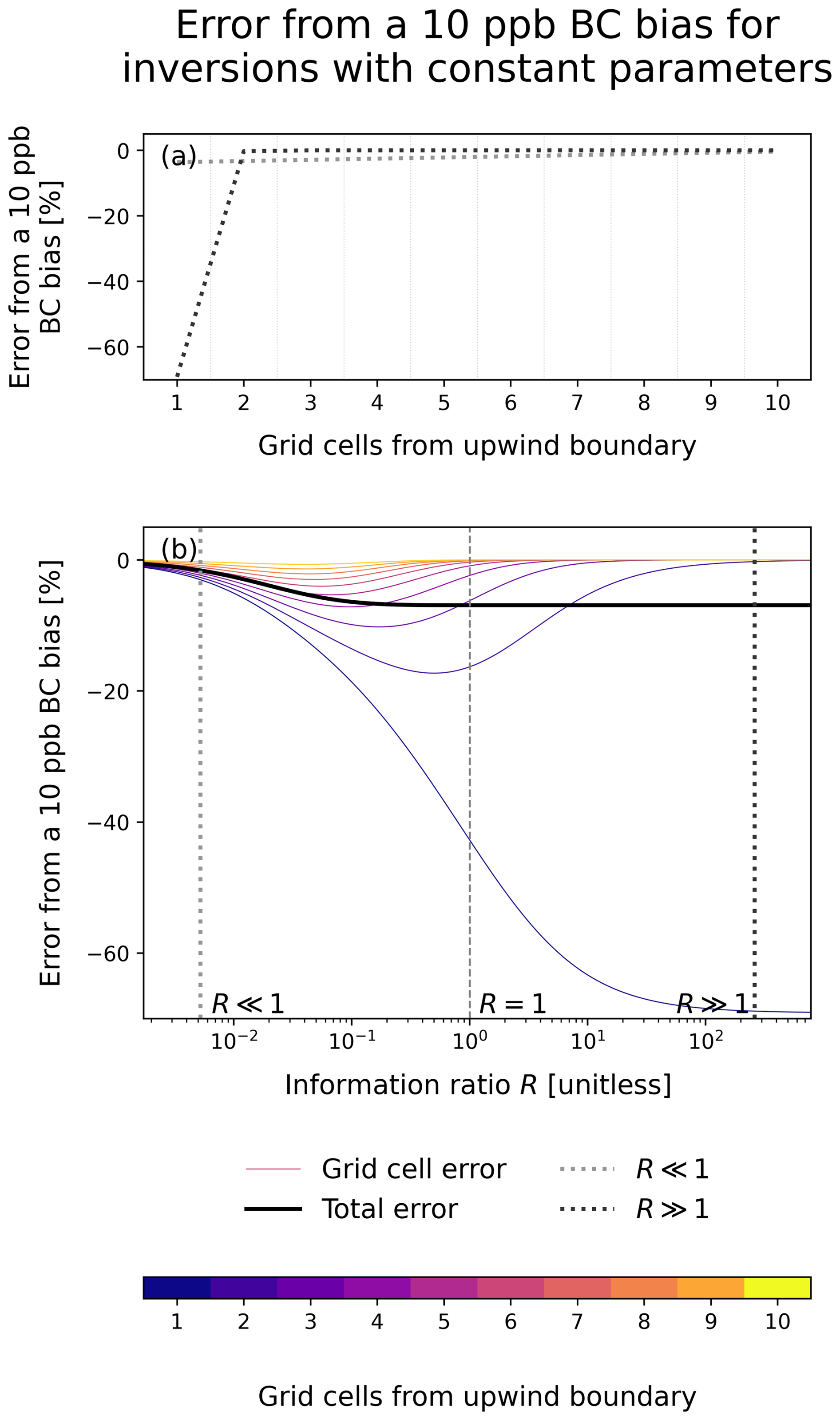
Figure 2 BC-induced error on posterior surface fluxes as a function of the information ratio R (Eq. 7) for a one-dimensional atmospheric trace gas inversion over ten grid cells with constant parameters. The inversions assume τ=1.4 h corresponding to $U=\mathrm{5}\mathrm{m}{\mathrm{s}}^{-\mathrm{1}}$ and L=25. The solid lines (b) represent the error induced by a 10 ppb BC bias relative to the prior emissions of 25 ppb h⁻¹ in each grid cell (thin lines) and the total error integrated across the full domain (thick black line). The dashed line corresponds to an information ratio of 1, while the dotted lines show representative values for which the limiting cases described in Eq. (8) hold. The distribution of the BC-induced errors across the domain for these representative values is also shown (a).

We also consider the effect of inverse methods to decrease BC biases within the constant parameter, one-dimensional inverse model. We compare the effect of optimizing the BC concentrations (boundary method) or fluxes outside of the domain of interest (buffer method). The boundary method optimizes one or more terms corresponding to BC concentrations along with the domain fluxes (Lauvaux et al., 2012; Wecht et al., 2014; Hancock et al., 2025). The buffer method expands the inversion domain to optimize fluxes in outlying grid cells, which are allowed to vary unphysically to absorb BC biases and are excluded from the final analysis (Shen et al., 2021; Varon et al., 2022). Both approaches increase the state vector dimension, thereby altering the Jacobian matrix and prior error covariance matrix. The buffer method also applies large prior error standard deviations to the buffer grid cells, often by aggregating the buffer grid cells into large clusters.

We derive the conditions under which the boundary and buffer methods are equivalent for an inversion of a single grid cell. For the boundary method, we use a BC prior error standard deviation equal to the constant BC bias ε_C and update the Jacobian matrix to include the sensitivity of the grid cell average observation to the BC. For the buffer method, we add a buffer grid cell and scale its prior error standard deviation by a factor of p. We assume observations are equally distributed over both grid cells. We solve both inversions. The posterior fluxes are equivalent when

$$\begin{array}{}\text{(9)}& p={\displaystyle \frac{{\mathit{\epsilon }}_{\mathrm{C}}}{\mathit{\tau }{\mathit{\sigma }}_{\mathrm{A}}\sqrt{R+\mathrm{2}}}}.\end{array}$$

Assuming steady state and knowledge of the domain wind speed, the buffer scale factor p can be chosen so that buffer and boundary methods perform equivalently. The scale factor goes to infinity for very small values of the information ratio (observation limited) and to zero for very large values (observation rich). The dependence of the scale factor on residence time implies that the buffer method is more vulnerable to varying wind speeds than the boundary method.

2.3 Preview for boundary condition errors

Equation (5) can estimate the effect of BC-induced errors on the posterior solution once model transport is characterized by the construction of the Jacobian matrix. We estimate BC-induced errors to inform the choice of inversion domain before building the Jacobian matrix by applying Eq. (5) to a simple steady-state two-box model that generalizes a gridded flux inversion. Figure 1b and c depict the model. The domain has BC c and constant wind speed U. All grid cells have representative grid cell length L given the wind direction. We consider a grid cell (with index j) that is j grid cells from the domain boundary and define the upwind grid cell (with index j0) as the aggregate of the upwind j grid cells. We conduct an inversion of the average observations over these two grid cells $\mathit{y}=[y_{j_{\mathrm{0}}}{y}_j{]}^{\mathrm{T}}$ regularized by prior fluxes ${\mathit{x}}_{\mathrm{A}}=[x_{\mathrm{A},j_{\mathrm{0}}}{x}_{\mathrm{A},j}{]}^{\mathrm{T}}$. We define the prior error covariance matrix as

$$\begin{array}{}\text{(10)}& {\mathbf{S}}_{\mathrm{A}}=\left[\begin{array}{cc}{\mathit{\sigma }}_{\mathrm{A},j_{\mathrm{0}}}^{\mathrm{2}}& \mathrm{0}\\ \mathrm{0}& {\mathit{\sigma }}_{\mathrm{A},j}^{\mathrm{2}}\end{array}\right]\end{array}$$

and use an equivalent structure for the observing system error covariance matrix. We assume the observing system error standard deviations account for the reduction in error resulting from averaging the observations. The Jacobian matrix is derived by steady-state mass balance (Sect. S1) to be a function of τ (Eq. 6) given by

$$\begin{array}{}\text{(11)}& \mathbf{K}=\mathit{\tau }\left[\begin{array}{cc}j& \mathrm{0}\\ j& \mathrm{1}\end{array}\right].\end{array}$$

We solve for the effect of a constant BC bias ε_C=[ε_C ε_C]^T on the posterior flux in the grid cell of interest $\mathrm{\Delta }{\widehat{\mathit{x}}}_j$ by applying the diagnostic (Eq. 5) to compute $\mathrm{\Delta }\widehat{\mathit{x}}=[\mathrm{\Delta }{\widehat{\mathit{x}}}_{j-\mathrm{1}}\mathrm{\Delta }{\widehat{\mathit{x}}}_j{]}^{\mathrm{T}}$. This defines the preview

$$\begin{array}{}\text{(12)}& \mathrm{\Delta }{\widehat{\mathit{x}}}_j=-{\displaystyle \frac{\left({\mathit{\tau }}^{-\mathrm{1}}{\mathit{\epsilon }}_{\mathrm{C}}\right)R_j}{\mathrm{1}+R_j+\mathit{\beta }{R}_{j_{\mathrm{0}}}+R_j{R}_{j_{\mathrm{0}}}}}\end{array}$$

where $R_{j_{\mathrm{0}}}$ and R_j refer to the information ratio (Eq. 7) in the upwind and selected grid cell, respectively, with ${\mathit{\tau }}_{j_{\mathrm{0}}}=j\mathit{\tau }$, and

$$\begin{array}{}\text{(13)}& \mathit{\beta }={\displaystyle \frac{m_{\mathrm{g},j}}{m_{\mathrm{g},j_{\mathrm{0}}}}}+\mathrm{1}.\end{array}$$

Here, $m_{\mathrm{g},j_{\mathrm{0}}}$ and m_g,j refer to the number of observations in the upwind and selected grid cell, respectively, so that β represents the relative observation density across the grid cells. For grid cells abutting the boundary, all upwind values are set to 0 so that the BC-induced error approaches τ⁻¹ε_C when the grid cell information ratio is large and 0 when the grid cell information ratio is small. As distance from the boundary increases, the BC-induced errors on average decrease due to the accumulation of upwind fluxes and observations, which increases the upwind information ratio $R_{j_{\mathrm{0}}}$. Variability in the prior fluxes and observation density as quantified by the information ratio R_j is super-imposed on this decay.

By analogy to our one-dimensional model, we consider the observation-limited and observation-rich limiting cases assuming constant prior fluxes, prior flux standard deviations, observation density, and observing system errors. In this case, $R_{j_{\mathrm{0}}}=j^{\mathrm{4}}{R}_j$ due to the dependence on the number of grid cells j of the upstream observation count ($m_{\mathrm{g},j_{\mathrm{0}}}=j{m}_{\mathrm{g}}$), grid cell residence time (${\mathit{\tau }}_{j_{\mathrm{0}}}=j\mathit{\tau }$), and prior flux uncertainty (assuming the uncertainties are uncorrelated, ${\mathit{\sigma }}_{\mathrm{A},j_{\mathrm{0}}}={\mathit{\sigma }}_{\mathrm{A}}/\sqrt{j}$). The resulting BC-induced errors

$$\begin{array}{}\text{(14)}& \mathrm{\Delta }{\widehat{\mathit{x}}}_j=\left\{\begin{array}{ll}-\left({\mathit{\tau }}^{-\mathrm{1}}{\mathit{\epsilon }}_{\mathrm{C}}\right)R,& R\ll \mathrm{1}\\ -\left({\mathit{\tau }}^{-\mathrm{1}}{\mathit{\epsilon }}_{\mathrm{C}}\right)j^{-\mathrm{4}}{R}^{-\mathrm{1}},& R\gg \mathrm{1}\end{array}\right.\end{array}$$

match the general form of the one-dimensional approximation (Eq. 8), but with the geometric decay in the observation-controlled limiting case approximated as quartic decay.

3 One-dimensional numerical solution

We demonstrate the preview, diagnostic, and correction methods using illustrative, numerical inversions of a one-dimensional model for the horizontal transport of an inert trace gas (Sect. 2.2; Nesser, 2025). Table S1 in the Supplement summarizes the model parameters and Table 1 the inversion parameters, which we select to simulate realistic inversions. We use these demonstration inversions to illustrate the effect of constant BC biases in inversions with constant and varying wind speeds (Sect. 3.1). We then consider periodic BC biases (Sect. 3.2). We finally generalize the results by varying the parameter choice to understand the variables controlling BC-induced errors (Sect. 3.3).

3.1 Constant boundary condition perturbations

We quantify the sensitivity of posterior fluxes to BC biases by perturbing the true BC in our one-dimensional model, solving the inversion, and comparing the posterior fluxes to those generated by an inversion solved with the true BC (Nesser, 2025). The inversions apply no other sources of bias (including transport errors) to isolate the effect of BC biases. The domain-average information ratio R=0.2 for these demonstration inversions reflects the low DOFS achieved (5 for inversions with constant wind speeds and 7 for varying wind speeds) despite the uniformity and large number of observations (m=1000), consistent with real inversions (Varon et al., 2023).

Table 1 Inversion parameters for simulation experiments.

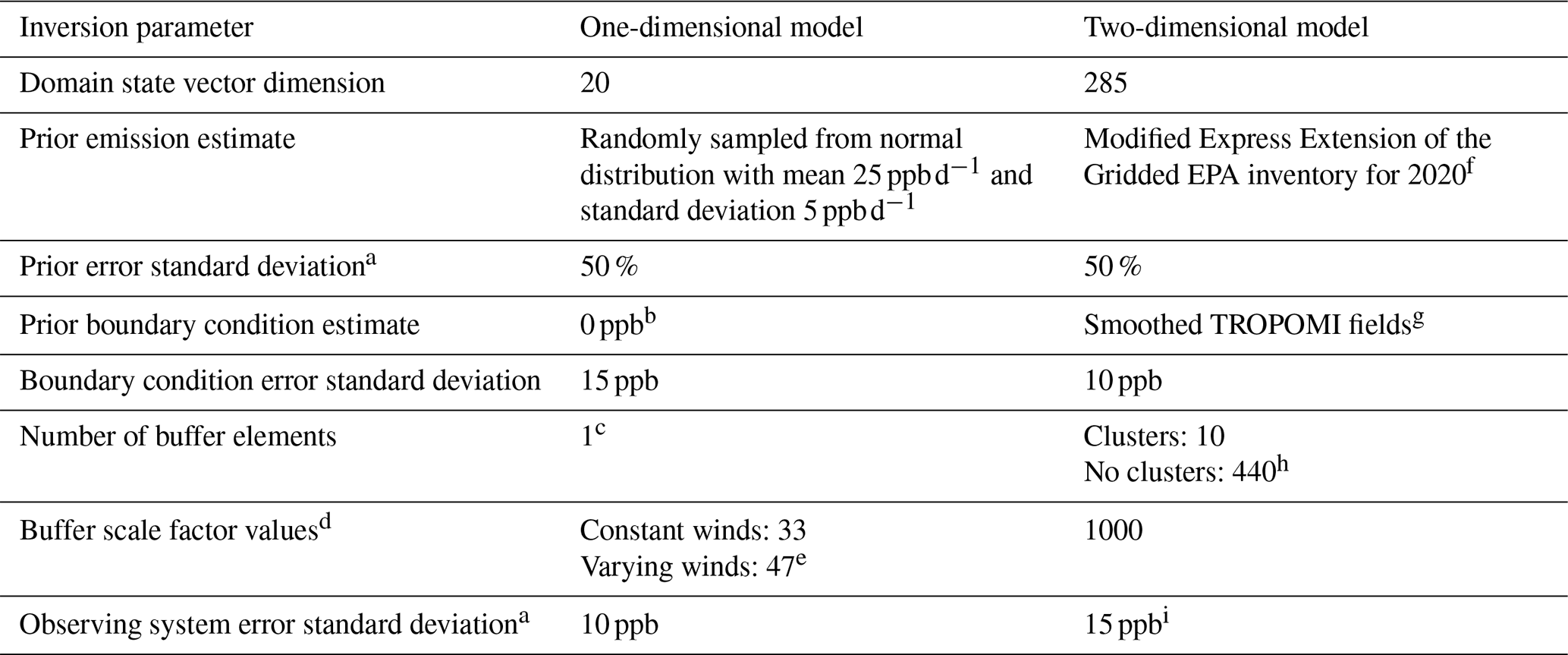
^a The error covariance matrices are assumed diagonal. ^b We optimize an incremental correction to the BC. ^c We optimize one buffer element that is a cluster of three native-resolution grid cells. ^d The buffer scale factor is the factor p applied to the prior error standard deviation in the buffer grid cell. ^e We calculate the buffer scale factor with Eq. (9). ^f We increase the Express Extension of the Gridded EPA inventory for 2020 (Maasakkers et al., 2023) by a factor of three so that the prior error statistics are consistent with the true emissions. ^g We use the IMI default boundary conditions, which are given by monthly mean TROPOMI observations smoothed over ≈1000 km. ^h We take as the inversion buffer zone the five concentric rings of 0.25°×0.3125° grid cells around the outer edge of the domain. We solve inversions using 10 buffer cluster elements and 440 native resolution buffer grid cells. ⁱ The IMI assumes a constant error standard deviation of 15 ppb for all observations aggregated into errors for the averaged observations accounting for error correlations following Chen et al. (2023). We use the errors generated by the IMI directly.

Figure 3a shows the relative difference in the posterior fluxes, normalized by the prior fluxes, induced by a constant 10 ppb BC perturbation for an inversion with constant wind speeds. As expected from our theoretical analysis, the resulting error on average decreases as the distance from the upwind boundary increases. Exceptions to the decreasing trend result from normalizing by the prior fluxes. The preview (Eq. 12) accurately predicts the error as expected from the specification of the wind speed. The diagnostic (Eq. 5; not shown) perfectly quantifies the no correction method error as expected given the specification of the BC bias.

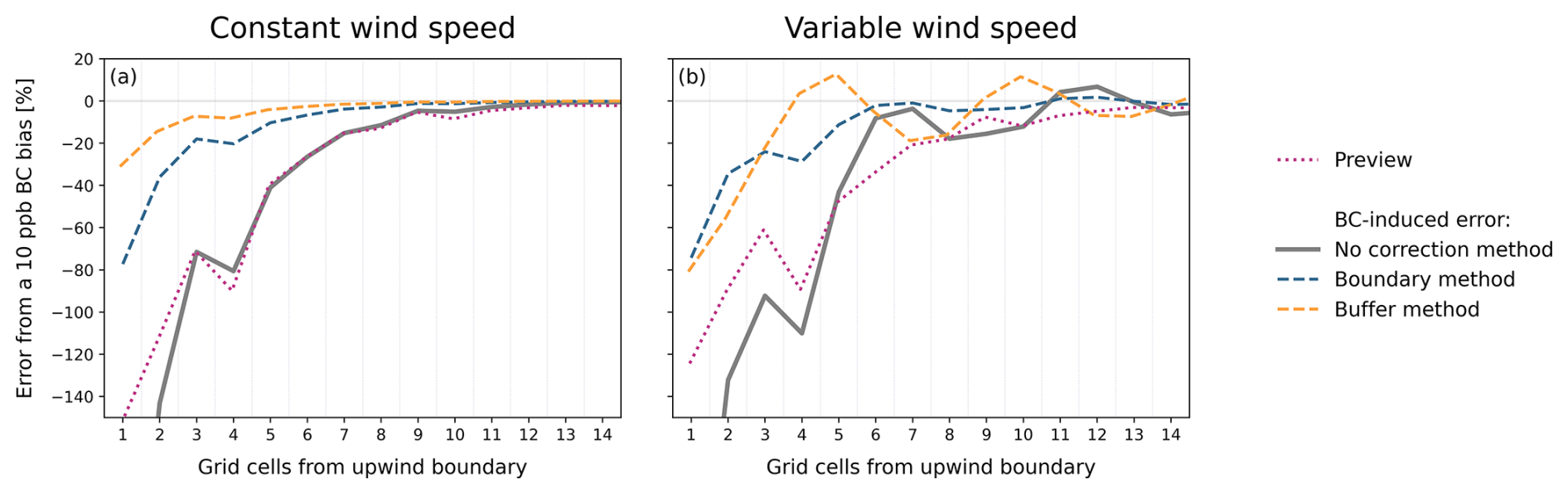
Figure 3 Exact and predicted influence of a constant BC bias on the posterior fluxes generated by a one-dimensional inverse model using different BC correction methods. The lines represent the posterior error induced by a 10 ppb BC perturbation as a function of the number of grid cells from the upwind boundary using constant (a) and varying (b) wind speeds. The error is given as the difference between inversions solved with the true and biased BCs, normalized by the prior fluxes ($\mathrm{\Delta }\widehat{\mathit{x}}/{\mathit{x}}_{\mathrm{A}}$). The error is shown for inversions solved with no BC correction method, the boundary method, and the buffer method. The buffer grid cell is not shown. The panels also show the preview. Only the first 13 of 20 grid cells are shown; all errors approach zero after this point. The varying wind speed is a see-sawing wind with mean equal to the constant wind speed.

Figure 3a also shows the effect of the buffer and boundary methods, which are described in Table 1. The buffer method optimizes a buffer cluster of three native resolution grid cells. Increasing the buffer grid cell size decreases the magnitude of BC-induced errors but increases the computational cost. The prior uncertainties of the buffer element are increased by a factor of 10p where p is the scale factor for which the boundary and buffer methods are theoretically equivalent (Eq. 9). Increasing p improves performance, but the error reduction quickly asymptotes so that a factor of 10 is sufficient to maximize error reduction in all tested cases. The boundary method optimizes an average correction to the BC.

Both the boundary and buffer methods reduce the error induced by the constant BC perturbation. The buffer method achieves larger uncertainty reductions than the boundary method as expected due to the choice of scale factor on the prior uncertainty. The uncorrected errors for the boundary method result from the decreased information available to correct the upwind fluxes, while the residual errors for the buffer method result from uncorrected BC biases. In all cases, the residual error magnitude, as measured by the root mean square error (RMSE) of the posterior fluxes compared to the inversion solved with the true BCs, is constant as a function of BC perturbation. This implies that the correction methods may increase posterior errors for grid cells close to the boundary in inversions with small BC biases. Excluding these grid cells from final analysis will minimize the effect of BC biases on the inversion.

The consistent performance of the metrics and of the correction methods results in part from the use of constant wind speeds, which is aligned with the assumptions used to derive the preview and the equivalence between the correction approaches. Figure 3b shows the effect of varying wind speeds. The BC-induced bias consists of decaying upwind biases and structured downwind biases. The preview (Eq. 12) accurately captures the average error decay over the domain, though it is unable to predict the structure of the downwind biases. The diagnostic (Eq. 5; not shown) perfectly predicts both the upwind and downwind biases due to its representation of transport and perfect knowledge of the BC bias. Both correction methods decrease the upwind biases, but only the boundary method decreases the downwind biases. Moreover, the RMSE of the posterior fluxes compared to the inversion solved with the true BCs is constant as a function of perturbation magnitude for the boundary method while the RMSE increases with perturbation magnitude for the buffer method. The buffer method is less able to decrease the variability of the BC-induced biases due to its dependence on wind speed (Eq. 9).

3.2 Varying boundary condition perturbations

Varying BC biases are unresolvable within inversions without prior knowledge of their structure. We consider variable BC biases to identify the types of biases that are most important to avoid, to understand the impact of correction methods, and to demonstrate the performance of the preview and diagnostic when the structure of the BC bias is not known. Because varying biases can be represented as the sum of periodic functions, we represent them with periodic BCs with varying y intercept, amplitude, and period number (Sect. S3 in the Supplement). The correction methods are implemented as in the constant perturbation case (Table 1 and Sect. 3.1) but with three BC elements optimized instead of one in the boundary method. This marginally increases the computational cost of the inversion but improves performance.

As in the inversion with a constant BC error and varying wind speeds, the periodic BC-induced bias consists of decaying upwind biases and structured downwind biases (Fig. S1 in the Supplement). The upwind biases are driven by the mean bias of the periodic perturbation over the inversion period. The spatial structure of the downwind biases is driven by the frequency of the BC error and the magnitude by the amplitude. This suggests that the correction methods will improve the upwind errors but not the downwind errors and that decreasing the amplitude of BC errors may reduce biases that are otherwise unresolvable.

Figure 4 shows the relative difference in the posterior fluxes, normalized by the prior fluxes, induced by a demonstration periodic perturbation with mean bias of 4 ppb over the inversion period (panel a and Sect. S3) for inversions with constant and varying wind speeds (panels b and c, respectively). The upwind biases are controlled by the mean bias with the error on average decreasing with the distance from the upwind boundary. The preview and diagnostic (Eqs. 13 and 5, respectively), which are calculated using the mean bias, capture these biases. The diagnostic also captures the downwind biases attributable to transport. Similarly, both correction methods decrease the upwind bias. The boundary method achieves modest error reductions because the BC-induced error is of similar magnitude to the error generated by the loss of information content due to the BC optimization. Downwind biases are only decreased by the boundary method when three or more BC elements are optimized.

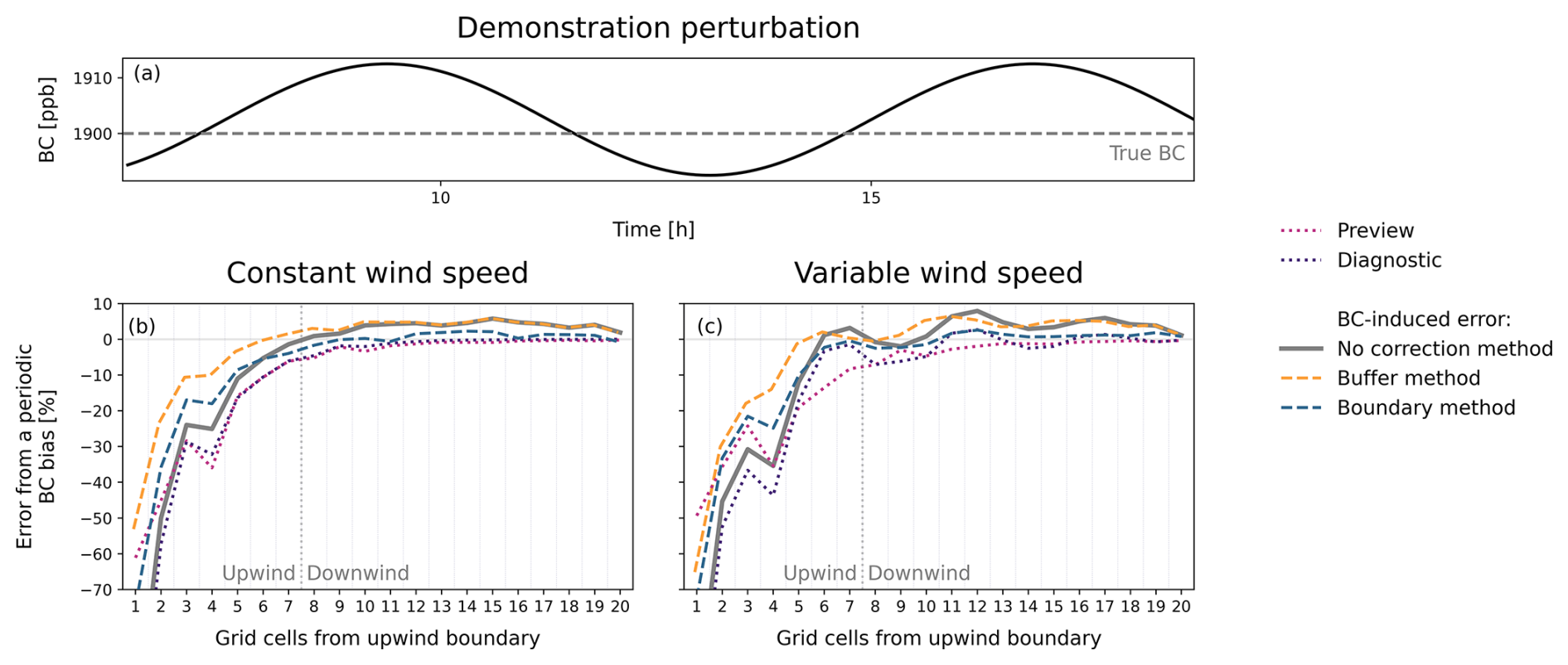
Figure 4 Exact and predicted influence of a periodic BC bias on the posterior fluxes generated by a one-dimensional inverse model using different BC correction methods. (a) shows the true and periodic BC. (b, c) show the posterior error induced by the periodic BC as a function of the number of grid cells from the upwind boundary error is given as the difference between inversions solved with the true and biased BCs, normalized by the prior fluxes ($\mathrm{\Delta }\widehat{\mathit{x}}/{\mathit{x}}_{\mathrm{A}}$) for constant and varying wind speeds, respectively. The error is shown for inversions solved with no BC correction method, the buffer method, and the boundary method. The buffer and boundary methods each optimize one additional element. The buffer grid cell is not shown. The panels also show the preview and diagnostic, which are calculated using the mean BC bias over the inversion period. The varying wind speed is a see-sawing wind with mean equal to the constant wind speed.

3.3 Varying inversion parameters

BC-induced posterior biases are a function of the relative constraint from the observations compared to the prior fluxes as measured by the information ratio (R, Eq. 7) and the grid cell residence time (τ, Eq. 6). To determine how changes in these quantities influence BC-induced biases, we define the influence length scale for our one-dimensional model as the number of grid cells required for the BC-induced error normalized by the prior fluxes to decrease below 0.25 ($\mathrm{\Delta }\widehat{\mathit{x}}/{\mathit{x}}_{\mathrm{A}}<\mathrm{0.25}$). The influence length scale captures the strong dependence of the BC-induced errors on the number of grid cells from the domain boundary and reflects the additional computational cost associated with optimizing these grid cells. We vary the mean prior flux (from 20–50 ppb h⁻¹) and associated prior error standard deviations, observation density (from 50–200 observations per grid cell), and mean wind speed (from 3–10 m s⁻¹) and calculate the domain average information ratio and residence time for each inversion. Uncertainty is quantified as the standard deviation of the influence length scale across 100 inversions solved with random prior fluxes. All inversions use varying wind speeds and a 10 ppb BC perturbation, though the results are robust for constant wind speeds.

Figure 5a shows the influence length scale as a function of the information ratio for an inversion with no correction method. As predicted from the one-dimensional model solved with constant parameters (Eq. 8 and Fig. 2), the influence length scale decreases with the information ratio. The largest rate of change occurs in the observation-limited regime as the observational constraint shifts the BC-induced errors into the upwind grid cells. In the observation-rich case, the influence length scale is relatively constant as a function of the information ratio. Figure 5b shows the inverse dependence of the influence length scale on grid cell residence time as predicted by Eq. (8). As residence time increases, the influence length scale decreases because the relative contribution of the fluxes compared to the BC increases in the observed concentrations, improving the observational constraint.

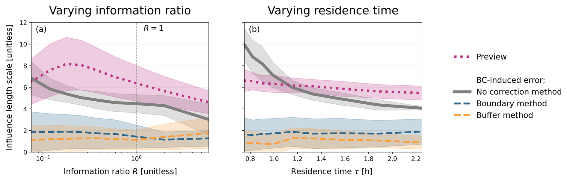
Figure 5 Sensitivity of the BC-induced posterior error to changes in parameters in a one-dimensional inverse model. The vertical axis shows the influence length scale defined as the number of grid cells before which the prior-normalized posterior errors resulting from a 10 ppb BC bias decrease below 0.25 ($\mathrm{\Delta }\widehat{\mathit{x}}/{\mathit{x}}_{\mathrm{A}}<\mathrm{0.25}$). The lines show the influence length scale for the preview and for inversions solved with no BC correction method, the boundary method, and the buffer method. Shading gives the one standard deviation range for 100 inversions solved with different random prior fluxes. (a) shows the influence length scale as a function of the information ratio R (Eq. 7) that describes the ratio of observing system error variances to the prior error variances in concentration units. The information ratio R=1 is marked by a vertical dashed line. (b) shows the influence length scale as a function of grid cell residence time (τ).

Finally, we consider the performance of the metrics and correction methods. The preview (Eq. 12) on average captures the dependence of the BC-induced error (no correction method) on the information ratio and grid cell residence time. In almost all cases, it marginally overestimates the influence length scale so that it represents an upper bound on error. As expected from the prescription of the BC perturbation, the diagnostic (not shown) perfectly predicts the influence length scale associated with no correction method. Both correction methods display functionally no dependence on the information ratio and grid cell residence time. The boundary and buffer methods comparably reduce the influence length scale in all cases.

4 Two-dimensional numerical solution

We extend the framework and understanding derived from the analytical solution and one-dimensional model to a two-dimensional demonstration inversion of TROPOMI-like methane column pseudo-observations over the Permian basin using the GEOS-Chem transport model as implemented by the Integrated Methane Inversion (IMI; Varon et al., 2022; Estrada et al., 2025; Nesser, 2025). The Permian Basin is the largest oil producing region in North America and the subject of many inverse analyses (e.g., Zhang et al., 2020; Barkley et al., 2023; Varon et al., 2023; Vanselow et al., 2024). Table S1 summarizes the model parameters, Table 1 gives the inversion parameters, and Fig. 6 shows the inversion domain, true emissions (panel a), prior emissions (panel b), and observation density as defined by real TROPOMI observations for May 2020 (panel c) for the n=285 grid cells within the inversion domain. The true BC is given by the IMI's TROPOMI-based smoothed BCs (Estrada et al., 2025). Assuming a constant wind speed of 5 m s⁻¹ and using average values of the prior and observing system error standard deviations, the domain average information ratio is R=0.03, reflecting the heterogeneous observational constraint.

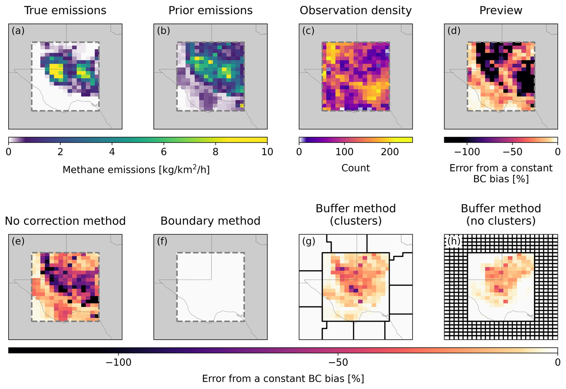
Figure 6 Exact and predicted influence of a constant BC bias on a two-dimensional simulation inversion over the Permian basin in Texas using different BC correction methods. True emissions from the Environmental Defense Fund high-resolution inventory (a; Zhang et al., 2020) and true BCs from smoothed TROPOMI observations are used to generate pseudo-observations over the Permian basin (dashed line) with observational density (c) given by the TROPOMI methane observations for May 2020. The inversion is regularized by prior emissions given by the Express Extension of the Gridded EPA Inventory for 2020 multiplied by a factor of three so that the prior error statistics include the true emissions (b; Maasakkers et al., 2023). The error induced by a spatially variable BC bias with mean 10 ppb is calculated as the difference between inversions solved with the true and biased BCs normalized by the prior fluxes. The error is shown for inversions solved with no correction method (e), the boundary method (f), and the buffer method using ten buffer clusters (g) and five rows of native resolution grid cells (h). The dark black outlines show the buffer clusters or grid cells where the prior uncertainties are artificially inflated and for which posterior fluxes are calculated but not shown. The preview (d) is also shown.

We apply a spatially variable BC bias of 7.5, 10, 10 and 12.5 ppb to the northern, southern, eastern, and western boundaries, respectively, using the Jacobian matrix for each edge of the domain as generated by the IMI. Figure 6e shows the resulting error in the posterior emissions normalized by the prior emissions. Unlike the BC-induced errors shown in the one-dimensional inversions, which used random prior fluxes, the distribution of the relative errors is strongly a function of the prior emissions. This likely results from the skewed distribution of the emissions across the domain, which limits the inversion's ability to correct fluxes near the domain edge.

The preview (Eq. 12) calculated with a BC uncertainty of 10 ppb is shown in Fig. 6d. We estimate the Jacobian matrix elements following Eq. (6) as implemented by Nesser et al. (2024) with a constant wind speed of 5 m s⁻¹, constant surface pressure of 1000 hPa, and a grid cell length scale given by the square root of each grid cell's area. We define the upwind length scale as the minimum distance from each grid cell's center to the border, dividing the domain into four regions based on proximity to each boundary. Upwind emissions and observation counts are calculated as the cumulative sum of the median value of each row or column between each grid cell and its closest boundary. Observing system errors are calculated by decreasing the 15 ppb single-observation uncertainty by the square root of the observation count. We apply a 5 ppb observing system error minimum to reflect transport and BC uncertainty.

The preview models the decay in BC-induced error as distance from the domain boundary increases accounting for the prior emission distribution and observation density (Eq. 12 and Sect. 2.3). As a result, the preview most accurately captures the effect of the BC bias nearest to the domain edge with a Pearson correlation coefficient of r=0.76 between the BC-induced biases and the preview for grid cells within three rows of the boundary. The performance of the preview degrades near the center of the domain, though there is still good agreement between the BC-induced biases and the preview for the full domain (r=0.67). The preview is larger than the BC-induced bias in most (63 %) of the grid cells so that the preview represents an error upper-bound. The diagnostic (not shown) perfectly captures the errors across the full domain as expected from the specification of the BC uncertainty.

Figure 6f, g, and h also show the correction methods. For the buffer method, we test two sets of buffer grid cells within the five concentric rings of grid cells around the outer edge of the domain. The first (clusters) aggregates the individual grid cells into 10 large buffer clusters using K-means clustering. The second (no clusters) uses 440 individual grid cells as buffers. In all cases, we scale the prior error standard deviation for the buffer elements by a factor of p=1000, which we find is sufficient to minimize BC-induced errors in all tested inversions. This very large, unphysical factor is chosen to compensate for the very small emissions around the edge of the Permian basin. For the boundary method, we optimize a mean bias correction along the northern, southern, eastern, and western boundaries.

The correction results mirror those found in the one-dimensional varying wind speed example. All correction methods decrease the BC-induced errors. Despite relying on fewer than half of the observations used by the buffer method, the boundary method virtually eliminates BC-induced errors while avoiding unphysical flux corrections and significantly decreasing computational cost by reducing the domain size. The buffer method with no clusters outperforms the buffer method with clusters, suggesting that multiple rows of buffer grid cells are preferable to large clusters. Larger numbers of buffer grid cells may also better absorb biases with higher resolution spatial variability.

5 Conclusions

We developed and demonstrated a framework to predict and correct the effect of BC biases on the optimal (posterior) gridded surface fluxes generated by regional inversions of atmospheric trace gas observations using a transport model. We proposed two metrics to predict BC-induced errors both before (preview) and after (diagnostic) the inversion is solved. The preview can inform the choice of inversion domain while the diagnostic improves posterior error quantification. We also considered two methods to correct BC biases as part of an inversion by optimizing the BC directly (boundary method) or by unphysically correcting grid cell fluxes outside the domain of interest (buffer method). Both methods can obtain identical error reductions in inversions with constant wind speeds, but the boundary method is more effective for inversions with variable wind speeds, provides a physical constraint, and reduces computational cost. Beyond the application to regional inversions of long-lived gases presented here, the framework is more generally applicable to the analysis of bias in the observations or transport model and the treatment of initial conditions in global inversions.

We demonstrated our theoretical framework using a simple one-dimensional model for the horizontal transport of an inert trace gas, which represents the worst-case scenario for the propagation of BC biases to the posterior flux estimate. BC-induced errors on average decay with increasing distance from the domain edge while smaller downwind systematic biases result from variability in the transport model wind speeds or BC biases. The length scale over which BC-induced errors have a significant effect on the posterior fluxes is minimized when the observations provide a strong constraint across the domain, which limits the bias to the most upwind grid cells. The preview identifies the grid cells with the largest biases, supporting domain specification before the inversion is conducted, while the diagnostic perfectly predicts the BC-induced error when the BC perturbation is specified. The boundary and buffer method both significantly reduce the influence length scale, but only the boundary method can decrease the magnitude of downwind errors. The results are robust for constant and variable BC biases.

We extended the framework to a two-dimensional demonstration inversion over the Permian Basin in Texas using model transport from the GEOS-Chem transport model. The BC-induced biases do not decay with distance from the boundary but instead correlate with the prior flux estimate due to the concentration of emissions in the center of the domain. Despite the difference in the distribution of BC-induced biases compared to the one-dimensional model, we find similar performance of the metrics and correction methods. The preview accurately predicts the BC-induced errors, with the best agreement occurring in the grid cells closest to the domain boundary. The diagnostic accurately describes the errors across the full domain. The boundary method functionally eliminates the BC-induced errors at much lower computational cost despite relying on fewer than half of the observations used in the buffer method. The buffer method decreases but does not eliminate BC-induced errors, with performance improving as the number of buffer clusters increases.