Development of the global maize yield model MATCRO-Maize version 1.0

Process-based crop models combined with land surface models are useful tools for accurately quantifying the impacts of climate change on crops while considering the interactions between agricultural land and climate. MATCRO model is a process-based crop model initially developed for paddy rice, combined with a land surface model. We developed MATCRO-Maize as a new model for maize by incorporating leaf-level photosynthesis of C₄ plants and adjusting crop-specific parameters into the original MATCRO model. MATCRO-Maize was evaluated at both a point scale and a global scale through comparisons with observational values. For global-scale simulations, the simulated yield showed statistically significant differences compared with Food and Agriculture Organization's FAOSTAT data at the country and global levels. Although the absolute value of the simulated yield tended to be overestimated, MATCRO-Maize reproduced spatial patterns with a correlation coefficient (COR) of 0.58 (p value < 0.01) for the 30-year average yield comparison of the top 20 maize-producing countries. In addition, the comparisons of the interannual variability derived from detrended deviation were statistically significant for the total global yield (COR of 0.55 with p value < 0.01) and for half of the top 20 countries (COR of 0.64–0.90 with p value < 0.001 for 6 countries; COR of 0.50–0.51 with p value < 0.01 for 2 countries; COR of 0.48–0.55 with p value < 0.05 for 2 countries), which are comparable with those of other global crop models. One of the reasons for this overestimation could be related to the strong model response to nitrogen fertilizer observed in MATCRO-Maize. With experimental field data under more comprehensive conditions, improvements in the functions of nitrogen fertilizer in the model would be needed to simulate the maize yield more accurately.

1 Introduction

Maize (Zea mays L.) is one of the most important cereals not only because of its large production (FAO, 2022) but also because of its various roles in human food, feed, and industrial uses. Maize exhibits high photosynthetic efficiency due to its C₄ plant nature. It contains phosphoenolpyruvate (PEP) carboxylase in mesophyll cells, which concentrates CO₂ in bundle sheath cells. The concentrated CO₂ increases the relative amount of carboxylation versus oxygenation performed by ribulose-1,5-bisphosphate carboxylase/oxygenase (Rubisco) (Kanai and Edwards, 1999), allowing C₄ plants to operate at lower stomatal conductance rates than C₃ plants (Sage, 1999). This mechanism results in high efficiencies of light, water, and nitrogen use (Knapp and Medina, 1999; Long, 1999). These features, such as multipurpose crops and high photosynthetic efficiency, enable the cultivated area to range over wide environments from wet to dry and from low to midlatitudes. However, climate change impacts and climate-related extremes negatively affect the productivity of the agricultural sector, which leads to negative consequences for food security (IPCC, 2023). Therefore, it is important to accurately quantify the impact of climate change on crop growth and yield and to identify effective adaptation strategies to mitigate climate risk.

Process-based crop models are useful tools for climate change studies because they consider the response of the physiological processes of crop growth and development to the environment and management (Tubiello and Ewert, 2002). The ensemble of process-based crop model simulations has shown good agreement with observed maize yields both at the site scale and at the global scale (Bassu et al., 2014; Jägermeyr et al., 2021), showing its potential to quantify the uncertainty in studies on the impacts of climate change on crop yields (Asseng et al., 2013). Crop models combined with Land Surface Models (LSMs) or Earth System Models (ESMs) (as classified by Peng et al., 2018) have the ability to consider the effects of agricultural land on the climate globally through the exchange of fluxes of heat, water, and gases, as well as the effects of climate on crops. Some studies have revealed that agricultural land affects the climate through fluxes (Bondeau et al., 2007; Levis et al., 2012; Maruyama and Kuwagata, 2010; Tsvetsinskaya et al., 2001) and subsequently affects crop production (Osborne et al., 2009). This indicates the importance of considering the interaction between agricultural land and climate to accurately quantify the impacts of climate change on crops. Despite this importance, few LSM/ESM-based crop models exist (Lin et al., 2021; Lombardozzi et al., 2020; Osborne et al., 2015; Wu et al., 2016).

MATCRO is a process-based crop growth model developed for C₃ plants (Masutomi et al., 2016a, b; Yusara et al., 2025). It was initially combined with a land surface model of Minimal Advanced Treatments of Surface Interaction and Runoff, called MATSIRO (Takata et al., 2003). MATSIRO is embedded in an ESM, which is the Model for Interdisciplinary Research on Climate, Earth System version 2 for Long-term simulations called MIROC-ES2L (Hajima et al., 2020). MATCRO simulates crop growth based on leaf-level photosynthesis and parameterized crop-specific parameters determined from experimental data, and it can run simulations both at a point scale and at a global scale. The model was applied to assess the impact of climate change at the country and local levels (Kinose et al., 2020; Kinose and Masutomi, 2019), and it was used in a study investigating factors to improve the simulation performance of global gridded crop models (GGCMs) (Iizumi et al., 2021). MATCRO is applicable to other crops, including maize as a C₄ plant, with adjusted parameters from experimental datasets and the literature.

We extended MATCRO for global maize yield simulation, called MATCRO-Maize, by adjusting crop-specific parameters for maize and incorporating the C₄ photosynthetic mechanism. The original model of MATCRO-Rice can simulate latent heat flux, sensible heat flux, net carbon uptake by crops, and rice yield, indicating its application in studies on climate change impacts as an LSM-based model (Masutomi et al. 2016b). However, this study focused only on crop growth and yields, omitting water and heat fluxes to increase computational efficiency. This paper aims to describe the methodology of MATCRO-Maize in detail (Sect. 2), to evaluate simulated yields both at a point scale and at a global scale with reference datasets (Sect. 3), and to provide discussion of the evaluation and model limitations (Sect. 4).

2 Model description

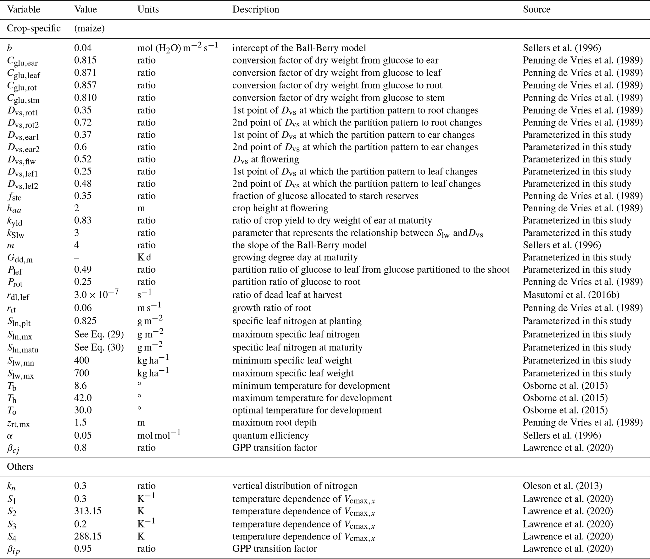
MATCRO consists of four modules: radiation, net carbon assimilation, crop growth, and soil water balance. It requires the following input data: (i) phenological data (i.e., crop calendar), (ii) water management data (i.e., the land is rainfed or irrigated), (iii) nitrogen fertilizer application data (N_fert) [kg N ha⁻¹], (iv) soil classification data (i.e., soil texture classification), (v) annual CO₂ data [ppm], and (vi) 6 types of daily meteorological data: air pressure (P_s) [Pa], precipitation (P_rc) [kg m⁻² s⁻¹], specific humidity [S_h] [kg kg⁻¹], downwards shortwave radiation (R_s) [W m⁻²], maximum, minimum, and mean air temperature (T_max, T_min, T_a) [K], and wind speed (U) [m s⁻¹]. Based on input data, MATCRO simulates crop growth during a growing period. It is controlled by the crop developmental stage (D_vs) based on (Bouman et al., 2001), which is the index used to quantify crop development. The final crop yield is determined by the dry weight of the storage organ with a parameter (K_yld) when D_vs=1. To adapt MATCRO for maize, crop-specific parameters and equations were improved, as shown in Table 1 and Eqs. (1)–(35). The details are described in the following sections.

Table 1 Parameters in MATCRO-Maize.

2.1 Photosynthetic mechanism

MATCRO-Maize calculates net carbon assimilation for the entire canopy (A_n) via the big-leaf model, where C₄ leaf-level photosynthesis is separately calculated for sunlit and shaded leaves from the coupled photosynthesis-stomatal conductance model (Collatz et al., 1991; Dai et al., 2004).

A_n for the entire canopy is given by:

$$\begin{array}{}\text{(1)}& A_n={\stackrel{\mathrm{‾}}{A}}_{n,\mathrm{sn}}{L}_{\mathrm{sn}}+{\stackrel{\mathrm{‾}}{A}}_{n,\mathrm{sh}}{L}_{\mathrm{sh}},\end{array}$$

where ${\stackrel{\mathrm{‾}}{A}}_{n,\mathrm{sn}}$ and ${\stackrel{\mathrm{‾}}{A}}_{n,\mathrm{sh}}$ represent the net carbon assimilation per unit leaf area [µmol m⁻² s⁻¹]; L_sn and L_sh represent the leaf area index (LAI) [m² (leaf) m⁻²]; and sn and sh indicate sunlit and shaded leaves, respectively. ${\stackrel{\mathrm{‾}}{A}}_{n,\mathrm{sn}}$ and ${\stackrel{\mathrm{‾}}{A}}_{n,\mathrm{sh}}$ are defined in the following equations:

$$\begin{array}{}\text{(2)}& {\stackrel{\mathrm{‾}}{A}}_{n,x}={\stackrel{\mathrm{‾}}{A}}_{\mathrm{g},x}-{\stackrel{\mathrm{‾}}{R}}_{\mathrm{d},x},\end{array}$$

where ${\stackrel{\mathrm{‾}}{A}}_{\mathrm{g},x}$ and ${\stackrel{\mathrm{‾}}{R}}_{\mathrm{d},x}$ represent gross carbon assimilation and dark respiration per unit leaf area [µmol m⁻² s⁻¹], respectively. Suffix x means sn or sh. L_sn and L_sh are determined following the approach of Masutomi et al., (2016a). ${\stackrel{\mathrm{‾}}{R}}_{\mathrm{d},x}$ is calculated via the following equation (Bonan et al., 2011):

$$\begin{array}{}\text{(3)}& {\stackrel{\mathrm{‾}}{R}}_{\mathrm{d},x}=\mathrm{0.025}{V}_{\mathrm{cmax},x}\left({\displaystyle \frac{{\mathrm{2}}^{\left(T_v-\mathrm{298.15}\right)/\mathrm{10}}}{\mathrm{1}+\exp \left(\mathrm{1.3}\right(T_v-\mathrm{328.15}\left)\right)}}\right),\end{array}$$

where V_cmax,x [µmol m⁻² s⁻¹] is the maximum rate of carboxylation and where T_v is the leaf temperature [K] (assumed to be the same as the air temperature: T_a).

${\stackrel{\mathrm{‾}}{A}}_{\mathrm{g},x}$ is determined by the smaller root of the following equations:

$$\begin{array}{}\text{(4)}& {\displaystyle }{\mathit{\beta }}_{cj}{\stackrel{\mathrm{‾}}{A}}_{i,x}^{\mathrm{2}}-\left({\stackrel{\mathrm{‾}}{A}}_{c,x}+{\stackrel{\mathrm{‾}}{A}}_{j,x}\right){\stackrel{\mathrm{‾}}{A}}_{i,x}+{\stackrel{\mathrm{‾}}{A}}_{c,x}{\stackrel{\mathrm{‾}}{A}}_{j,x}=\mathrm{0},\text{(5)}& {\displaystyle }{\mathit{\beta }}_{ip}{\stackrel{\mathrm{‾}}{A}}_{\mathrm{g},x}^{\mathrm{2}}-\left({\stackrel{\mathrm{‾}}{A}}_{i,x}+{\stackrel{\mathrm{‾}}{A}}_{p,x}\right){\stackrel{\mathrm{‾}}{A}}_{\mathrm{g},x}+{\stackrel{\mathrm{‾}}{A}}_{i,x}{\stackrel{\mathrm{‾}}{A}}_{p,x}=\mathrm{0},\end{array}$$

where β_cj and β_ip are the transition factors (Table 1) and where ${\stackrel{\mathrm{‾}}{A}}_{i,x}$ [µmol m⁻² s⁻¹] is the carbon fixation rate. Here, we introduced the C₄ leaf-level photosynthesis model based on Collatz et al. (1992) into MATCRO, in which some parameters were taken from Oleson et al. (2013) and Lawrence et al. (2020) (see Table 1). In C₄ photosynthesis, ${\stackrel{\mathrm{‾}}{A}}_{c,x}$, ${\stackrel{\mathrm{‾}}{A}}_{j,x}$, and ${\stackrel{\mathrm{‾}}{A}}_{p,x}$ [µmol m⁻² s⁻¹] represent Rubisco-limited, RUBP-limited, and PEP-limited photosynthesis, respectively, and are given by the following equations:

$$\begin{array}{}\text{(6)}& {\displaystyle }{\stackrel{\mathrm{‾}}{A}}_{c,x}=V_{\mathrm{cmax},x},\text{(7)}& {\displaystyle }{\stackrel{\mathrm{‾}}{A}}_{j,x}=\mathit{\alpha }\left(\mathrm{4.6}{Q}_{\mathrm{ab},x}\right),\text{(8)}& {\displaystyle }{\stackrel{\mathrm{‾}}{A}}_{p,x}=k_{p,x}{C}_{\mathrm{i},x},\end{array}$$

where Q_ab,x [W m⁻²] is the absorbed photosynthetically active radiation (PAR); α [mol mol⁻¹] is the quantum efficiency; k_p,x [mol m⁻² s⁻¹] is the initial slope of the CO₂ response curve for the C₄ CO₂ response curve; and C_i,x [ppm] is the internal leaf CO₂ concentration. Q_ab,x is calculated from R_s via the same methods conducted in Masutomi et al. (2016a) and is converted to photosynthetic photon flux by multiplying by 4.6 [µmol (photons) J⁻¹]. V_cmax,x and k_p,x are functions of T_v and are based on Lawrence et al. (2020),

$$\begin{array}{}\text{(9)}& {\displaystyle }{V}_{\mathrm{cmax},x}=f_v{V}_{\mathrm{cmax}\mathrm{25},x}\left[{\displaystyle \frac{Q_{\mathrm{10}}^{(T_v-\mathrm{298.15})/\mathrm{10}}}{f_{\mathrm{H}}\left(T_v\right)f_{\mathrm{L}}\left(T_v\right)}}\right],\text{(10)}& {\displaystyle }{f}_{\mathrm{H}}\left(T_v\right)=\mathrm{1}+\exp \left[S_{\mathrm{1}}\left(T_v-S_{\mathrm{2}}\right)\right],\text{(11)}& {\displaystyle }{f}_{\mathrm{L}}\left(T_v\right)=\mathrm{1}+\exp \left[S_{\mathrm{3}}\left(S_{\mathrm{4}}-T_v\right)\right],\text{(12)}& {\displaystyle }{k}_{p,x}=\left\{\begin{array}{l}{k}_{p\mathrm{25},x}{Q}_{\mathrm{10}}^{(T_v-\mathrm{298.15})/\mathrm{10}},V_{\mathrm{cmax}\mathrm{25},x}>\mathrm{0},\\ \mathrm{0.7},V_{\mathrm{cmax}\mathrm{25},x}=\mathrm{0},\end{array}\right.,\text{(13)}& {\displaystyle }{k}_{p\mathrm{25},x}=\mathrm{20000}{V}_{\mathrm{cmax}\mathrm{25},x},\end{array}$$

with Q₁₀=2, S₁=0.3 K⁻¹, S₂=313.15 K, S₃=0.2 K⁻¹, and S₄=288.15 K (see Table 1). Notably, k_p,x is adjusted to be 0.7 mol  m⁻² s⁻¹ (Collatz et al., 1992) when $V_{\mathrm{cmax}\mathrm{25},x}=\mathrm{0}$ because of the process of the photosynthesis calculation (see Eq. 20). V_cmax25,x is the maximum Rubisco carboxylation rate per unit leaf area at 25° (the details are described in Sect. 2.2.2). f_H(T_v) and f_L(T_v) are modulating functions that reduce V_cmax,x at high and low temperatures, respectively. f_v is the water stress factor calculated in the soil water balance module, which indirectly affects A_n through V_cmax,x (Sellers et al., 1996). f_v is derived from the following equations:

$$\begin{array}{}\text{(14)}& {\displaystyle }{f}_v={\sum }_{i=\mathrm{1}}^{\mathrm{NSL}}\left\{\begin{array}{l}\mathrm{1}\times \mathrm{ETF}\left(i\right),\mathrm{FAW}\left(i\right)>\mathrm{0.45},\\ \frac{\mathrm{FAW}\left(i\right)}{\mathrm{0.45}}\times \mathrm{ETF}\left(i\right),\mathrm{otherwise},\end{array}\right.\text{(15)}& {\displaystyle }\mathrm{FAW}\left(i\right)=min\left({\displaystyle \frac{max\left(\left(\mathrm{WSL}\left(i\right)-\mathrm{WILT}\right),\mathrm{0}\right)}{\text{FC-WILT}}},\mathrm{1}\right)\text{(16)}& {\displaystyle }\mathrm{ETF}\left(i\right)={\displaystyle \frac{\mathrm{3}}{\mathrm{2}}}{\displaystyle \frac{(z_{\mathrm{rt}}^{\mathrm{2}}-z^{\mathrm{2}})}{z_{\mathrm{rt}}^{\mathrm{3}}}},\end{array}$$

where NSL represents the number of soil layers, ETF represents the fraction of transpiration from root distribution, FAW represents the fraction of available water, WSL represents the soil water content [m³ m⁻³], WILT represents the wilting point, FC represents the field capacity, and z_rt and z represent the root depth and the soil depth, respectively, for each layer. MATCRO assumes NSL =5, where each of the soil layers has depth of 0.05, 0.2, 0.75, 1, and 2 [m] below the ground, respectively. MATCRO uses the soil texture data as input data, where the soil is classified into 13 types, leading to differences in WILT and FC based on Campbell and Norman (1998). WSL is calculated considering transpiration from the canopy, evaporation from the soil, and water flux (those calculations are the same as those of the original MATCRO). The ETF calculation assumes that the root has no spatial orientation and is equally distributed in the soil (Masutomi et al., 2016a). z_rt is determined by the same calculation as the original MATCRO, where the crop-specific parameter (z_rt,mx) was changed to maize (Table 1). The conditional branch (FAW(i)>0.45) is based on the FAO 56 guidelines (Allen et al., 1998).

Stomatal conductance influences CO₂ uptake during photosynthesis. MATCRO-Maize represents stomatal conductance for CO₂ (G_sc,x [µmol m⁻² s⁻¹]), based on Ball (1988) as follows:

$$\begin{array}{}\text{(17)}& G_{\mathrm{sc},x}=\left\{\begin{array}{l}{G}_{\mathrm{0}c}+G_{\mathrm{1}\mathrm{c}}{R}_{\mathrm{h}}\frac{{\stackrel{\mathrm{‾}}{A}}_{n,x}}{C_{\mathrm{s},x}},{\stackrel{\mathrm{‾}}{A}}_{n,x}\ge \mathrm{0},\\ G_{\mathrm{0}c},\text{otherwise},\end{array}\right.\end{array}$$

where C_s,x [ppm] is the CO₂ concentration at the leaf surface and R_h [–] is the relative humidity at the leaf surface. G_0c and G_1c are derived from parameters of Ball-Berry stomatal conductance model of b and m (shown in Table 1) by adjusting their ratio of 1:1.6, which is the ratio of diffusivity of H₂O to CO₂. Here, the leaf-level net carbon assimilation rate (${\stackrel{\mathrm{‾}}{A}}_{n,x}$), stomatal conductance for CO₂ (G_sc,x), and boundary layer conductance for CO₂ (G_bc) were calculated to satisfy the following physical flux equations.

$$\begin{array}{}\text{(18)}& {\displaystyle }{\stackrel{\mathrm{‾}}{A}}_{n,x}=G_{\mathrm{sc},x}\left(C_{\mathrm{s},x}-C_{\mathrm{i},x}\right),\text{(19)}& {\displaystyle }{\stackrel{\mathrm{‾}}{A}}_{n,x}=G_{\mathrm{bc}}\left(C_{\mathrm{a}}-C_{\mathrm{s},x}\right),\end{array}$$

where C_a [ppm] is the atmospheric CO₂ concentration. G_bc is a function of air pressure (P_s [Pa]) and the wind speed in the canopy (U [m s⁻¹]).

Here, T_v, Q_ab,x, R_h, U, and C_a are environmental variables derived from input meteorological climate data. There are four relationships (Eqs. 2, 17–19) in terms of internal variables (${\stackrel{\mathrm{‾}}{A}}_{n,x}$, G_sc,x, C_s,x, C_i,x). MATCRO for C₃ photosynthesis obtains analytical solutions from relationships via the method shown in Masutomi (2023). For C₄ photosynthesis, it is also possible to solve these equations analytically. In the case of Rubisco-limited and RuBP-limited photosynthesis, exact expressions for ${\stackrel{\mathrm{‾}}{A}}_{c,x}$ and ${\stackrel{\mathrm{‾}}{A}}_{j,x}$ are obtained. Under ${\stackrel{\mathrm{‾}}{A}}_{n,x}\ge \mathrm{0}$, PEP-limited photosynthesis (${\stackrel{\mathrm{‾}}{A}}_{p,x}$) can be represented by quadratic equations by the algebraic procedures as follows:

$$\begin{array}{}\text{(20)}& \begin{array}{rl}\mathrm{0}& =\left\{G_{\mathrm{bc}}^{\mathrm{2}}{G}_{\mathrm{1}\mathrm{c}}{R}_{\mathrm{h}}-G_{\mathrm{bc}}{G}_{\mathrm{0}c}-k_{p,x}\left(G_{\mathrm{0}c}-G_{\mathrm{bc}}{G}_{\mathrm{1}\mathrm{c}}{R}_{\mathrm{h}}\right.\right.\\ & \left.\left.+G_{\mathrm{bc}}\right)\right\}{\stackrel{\mathrm{‾}}{A}}_{p,x}^{\mathrm{2}}+\left\{C_{\mathrm{a}}{G}_{\mathrm{bc}}^{\mathrm{2}}{G}_{\mathrm{0}c}-G_{\mathrm{bc}}{G}_{\mathrm{0}c}{R}_{\mathrm{d}}\right.\\ & +G_{\mathrm{bc}}^{\mathrm{2}}{G}_{\mathrm{1}\mathrm{c}}{R}_{\mathrm{h}}{R}_{\mathrm{d}}-k_{p,x}{C}_{\mathrm{a}}\left(G_{\mathrm{bc}}^{\mathrm{2}}{G}_{\mathrm{1}\mathrm{c}}{R}_{\mathrm{h}}-\mathrm{2}{G}_{\mathrm{bc}}{G}_{\mathrm{0}c}\right.\\ & \left.\left.-G_{\mathrm{bc}}^{\mathrm{2}}\right)\right\}{\stackrel{\mathrm{‾}}{A}}_{p,x}+C_{\mathrm{a}}{G}_{\mathrm{bc}}^{\mathrm{2}}{G}_{\mathrm{0}c}\left(R_{\mathrm{d}}-k_{p,x}{C}_{\mathrm{a}}\right).\end{array}\end{array}$$

Under ${\stackrel{\mathrm{‾}}{A}}_{n,x}<\mathrm{0}$, the PEP-limited photosynthesis rate can be expressed as

$$\begin{array}{}\text{(21)}& {\stackrel{\mathrm{‾}}{A}}_{p,x}={\displaystyle \frac{k_{p,x}{C}_{\mathrm{a}}-R_{\mathrm{d}}}{\mathrm{1}+k_{p,x}\left(\frac{\mathrm{1}}{G_{\mathrm{bc}}}+\frac{\mathrm{1}}{G_{\mathrm{0}c}}\right)}}.\end{array}$$

According to these equations, in the case of PEP-limited photosynthesis, there are three possible solutions. Following the criteria described by Masutomi (2023), only one analytical solution can be selected when the following requirements are satisfied: (i) under ${\stackrel{\mathrm{‾}}{A}}_{n,x}\ge \mathrm{0}$, the solution must be a positive or zero real solution, and under ${\stackrel{\mathrm{‾}}{A}}_{n,x}<\mathrm{0}$, it must be a negative real solution; (ii) $G_{\mathrm{sc},x}>\mathrm{0}$; and (iii) C_i>0.

2.2 Crop-specific parameterization

2.2.1 Phenology

The crop growing period in MATCRO is expressed as D_vs based on Bouman et al. (2001). Here, D_vs=0 means sowing, and D_vs=1 means maturity (harvesting). It is calculated from the following equations:

$$\begin{array}{}\text{(22)}& {\displaystyle }{D}_{\mathrm{vs},\mathrm{i}}=G_{\mathrm{dd},i}/G_{\mathrm{ddm},i},\text{(23)}& {\displaystyle }{G}_{\mathrm{dd}}=\underset{\mathrm{0}}{\overset{t}{\int }}{D}_{vr}\mathrm{d}{t}^{\prime },\text{(24)}& {\displaystyle }{D}_{vr}=\left\{\begin{array}{l}\mathrm{0},T_t<T_{\mathrm{b}}\mathrm{|}{T}_{\mathrm{h}}\le T_t,\\ T_t-T_{\mathrm{b}},T_{\mathrm{b}}\le T_t<T_{\mathrm{o}},\\ \frac{\left(T_{\mathrm{b}}-T_{\mathrm{o}}\right)\left(T_t-T_{\mathrm{h}}\right)}{\left(T_{\mathrm{h}}-T_{\mathrm{o}}\right)},T_{\mathrm{o}}\le T_t<T_{\mathrm{h}},\end{array}\right.\end{array}$$

where G_dd,i is the growing degree days at t (time) for specific grid cell number i; G_ddm,i is the growing degree day at maturity; D_vr is the developmental rate at time t; and T_t is the temperature at time t. T_b, T_h, and T_o are the crop-specific cardinal temperatures (minimum, maximum, and optimal temperatures for development, respectively, as shown in Table 1). G_dd,m were calibrated for each point scale simulation and global scale simulation (Sect. 2.3). In addition, one parameter that represents the timing of flowering (known as silking; D_vs,flw) was calibrated based on observational data for the point scale simulation (Table 1).

2.2.2 Leaf nitrogen and Rubisco capacity

Maximum Rubisco carboxylation rate

V_cmax25,x used in the photosynthesis module (Sect. 2.1) is obtained by dividing the maximum Rubisco carboxylation rate at a LAI depth of l (V_cmax25,x(l)) by L_x separately for sunlit and shaded leaves based on Bonan et al. (2011). The vertical distribution of V_cmax25(l), which is the sum of V_cmax25,sn(l) and V_cmax25,sh(l), follows the exponential profile:

$$\begin{array}{}\text{(25)}& V_{\mathrm{cmax}\mathrm{25}}\left(l\right)=V_{\mathrm{cmax}\mathrm{25}}\left(\mathrm{0}\right)\exp \left(-K_{n}l\right),\end{array}$$

where V_cmax25(0) is the maximum Rubisco carboxylation rate at the canopy top, K_n is a parameter for the vertical distribution of nitrogen (Table 1), and l represents the LAI depth from the top. The maximum Rubisco carboxylation rate in sunlit leaves (V_cmax25,sn(l)) is also calculated by the same relationship considering the light distribution:

$$\begin{array}{}\text{(26)}& \begin{array}{rl}{V}_{\mathrm{cmax}\mathrm{25},\mathrm{sn}}\left(l\right)& =V_{\mathrm{cmax}\mathrm{25}}\left(\mathrm{0}\right)\left[\mathrm{1}-\exp \left(-l(K_n+K)\right)\right]\\ & {\displaystyle \frac{\mathrm{1}}{K_n+K}},\end{array}\end{array}$$

where K is the direct beam extinction coefficient (the calculation is the same as that for Masutomi et al., 2016a). V_cmax25,sh(l) is given by the subtraction of Eqs. (25) and (26).

Here, while Bonan et al. (2011) use the fixed value of V_cmax25(0) value over time, V_cmax25(0) in MATCRO is calculated dynamically as a function of specific leaf nitrogen (S_ln [g N m⁻²]). The function is established based on the experimental literature data. Notably, we applied the relationship between S_ln and light-saturated CO₂ assimilation (A_max) from the literature, although MATCRO-Rice and MATCRO-Soy utilize the direct relationship between S_ln and V_cmax25(0) based on the experimental literature data. The reasons are that we assume that A_max could be used as Rubisco-limited photosynthesis in C₄ photosynthesis, hence Rubisco-limited photosynthesis could be equal to the maximum Rubisco carboxylation rate from Eq. (6). Several studies have shown that A_max has a close relationship with S_ln, as shown by the logistic equation for maize (Drouet and Bonhomme, 2004; Muchow and Sinclair, 1994; Paponov and Engels, 2003; Paponov et al., 2005; Sinclair and Horie, 1989; Vos et al., 2005). We used two functions from the studies for different D_vs as follows:

$$\begin{array}{}\text{(27)}& \begin{array}{rl}& V_{\mathrm{cmax}\mathrm{25}}\left(\mathrm{0}\right)=\\ & \left\{\begin{array}{l}\mathrm{45.1}\times \left\{\frac{\mathrm{2}}{\mathrm{1}+\exp \left[-\mathrm{2.9}\cdot \left(S_{\ln }-\mathrm{0.25}\right)\right]}-\mathrm{1}\right\},D_{\mathrm{vs}}<D_{\mathrm{vs},\mathrm{flw}},\\ \mathrm{40.2}\times \left\{\frac{\mathrm{2}}{\mathrm{1}+\exp \left[-\mathrm{1.41}\cdot \left(S_{\ln }-\mathrm{0.43}\right)\right]}-\mathrm{1}\right\},\text{otherwise},\end{array}\right.\end{array}\end{array}$$

where $D_{\mathrm{vs}}<D_{\mathrm{vs},\mathrm{flw}}$ represents the vegetative stage at which the equation was based on Vos et al. (2005); then, for the reproductive stage, the equation was from Drouet and Bonhomme (2004). Stage-specific parameterizations were applied to reflect the lower photosynthetic activity observed during the reproductive phase compared to the vegetative phase since no single dataset adequately represents both growth phase.

Specific leaf nitrogen

S_ln, which is used in the calculation of V_cmax25(0), is dynamically change during the crop growth of D_vs in MATCRO. The function is established based on the observational data. We utilized the study by Muchow (1988), in which S_ln was measured under various levels of N_fert (0, 60, 120, 240, 420 [kg ha⁻¹]), as follows: (i) we traced S_ln data using digitizer software (https://apps.automeris.io/wpd4/, last access: 20 November 2024) and obtained the measurement and phenological data from the paper; and (ii) we conducted the fitting based on the assumption that S_ln linearly increased until flowering and then decreased towards maturity. The parameterization given by Eqs. (28)–(30) is shown in Fig. 1.

$$\begin{array}{}\text{(28)}& \begin{array}{rl}& S_{\ln }=\\ & \left\{\begin{array}{l}\frac{S_{\ln ,\mathrm{mx}}-S_{\ln ,\mathrm{plt}}}{D_{\mathrm{vs},\mathrm{flw}}}{D}_{\mathrm{vs}}+S_{\ln ,\mathrm{plt}},D_{\mathrm{vs}}<D_{\mathrm{vs},\mathrm{flw}},\\ \frac{S_{\ln ,\mathrm{matu}}-S_{\ln ,\mathrm{mx}}}{\mathrm{1}-D_{\mathrm{vs},\mathrm{flw}}}\left(D_{\mathrm{vs}}-\mathrm{1}\right)+S_{\ln ,\mathrm{matu}},D_{\mathrm{vs}}\ge D_{\mathrm{vs},\mathrm{flw}}.\end{array}\right.\end{array}\end{array}$$

Where S_ln,mx, S_ln,plt, S_ln,matu are maximum S_ln, and S_ln at planting time and maturity, respectively. S_ln,plt was parameterized by assuming low S_ln in the early stage (Table 1). Menwhile, S_ln,mx and S_ln,matu are empirically parameterized as functions of N_fert as follows:

$$\begin{array}{}\text{(29)}& {\displaystyle }\begin{array}{rl}& S_{\ln ,\mathrm{mx}}=\\ & \left\{\begin{array}{l}-\mathrm{0.00001}{N}_{\mathrm{fert}}^{\mathrm{2}}+\mathrm{0.0064}{N}_{\mathrm{fert}}+\mathrm{0.6891},N_{\mathrm{fert}}\le \mathrm{240},\\ \mathrm{1.75},N_{\mathrm{fert}}>\mathrm{240}.\end{array}\right.\end{array}\text{(30)}& {\displaystyle }{S}_{\ln ,\mathrm{matu}}=\left\{\begin{array}{l}\mathrm{0.001}{N}_{\mathrm{fert}}+\mathrm{0.57},N_{\mathrm{fert}}\le \mathrm{240},\\ \mathrm{1},N_{\mathrm{fert}}>\mathrm{240}.\end{array}\right.\end{array}$$

We set fixed values of 1.75 for S_ln,mx and 1.0 for S_ln,matu when N_fert exceeds 240 [kg ha⁻¹], as S_ln,mx and S_ln,matu exhibit minimal increases beyond this threshold.

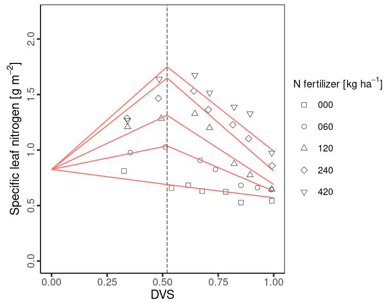
Figure 1 Relationship between developmental stage (D_vs) and specific leaf nitrogen (S_ln) in MATCRO-Maize. Symbols show observational data from Muchow (1988) with the 5 types of N_fert: 0 kg ha⁻¹ (square), 60 kg ha⁻¹ (cycle), 120 kg ha⁻¹ (triangle), 240 kg ha⁻¹ (diamond), and 420 kg ha⁻¹ (inverted triangle). The red lines represent the fitted line parameters used in MATCRO-Maize, while the dashed line represents D_vs at flowering (D_flw).

2.2.3 Crop growth

Glucose partitioning

MATCRO calculates crop growth by partitioning net carbon assimilation (A_n) in the form of glucose, which is calculated in the photosynthesis module (Sect. 2.1). Partitioned glucose is supplied through photosynthesis in leaves and remobilization from the stem. The ratio of glucose partition to each organ (leaf, stem, root, and storage organ; ear) depends on D_vs. The term “ear” in maize represents the organ that supports the development and storage of grain. The grain developed later than the ear with approximately 83 % of ear at maturity in this study (see Sect. 2.2.5). The dry matter for each organ is obtained from the partitioned glucose considering the carbon fraction for each organ (C_glu,ear, C_glu,leaf, C_glu,rot, C_glu,stm in Table 1). We calibrated the partitioning ratio to leaf and ear based on the observational biomass data from Ciampitti et al. (2013a, b), whereas the ratio to shoots:roots was derived from the value from Penning de Vries et al. (1989). The stem partitioning was determined by reducing the shoot ratio with respect to the leaf and ear. Figure 2 shows the partition ratio to the leaf (P_r,lef) and ear (P_r,ear) established via the following equations:

$$\begin{array}{}\text{(31)}& {\displaystyle }{P}_{\mathrm{r},\mathrm{lef}}=\left\{\begin{array}{l}{P}_{\mathrm{lef}},D_{\mathrm{vs}}<D_{\mathrm{vs},\mathrm{lef}\mathrm{1}},\\ \frac{P_{\mathrm{lef}}(D_{\mathrm{vs},\mathrm{lef}\mathrm{2}}-D_{\mathrm{vs}})}{D_{\mathrm{vs},\mathrm{lef}\mathrm{2}}-D_{\mathrm{vs},\mathrm{lef}\mathrm{1}}},D_{\mathrm{vs}}<D_{\mathrm{vs},\mathrm{lef}\mathrm{2}}\\ \mathrm{0},\text{otherwise},\end{array},\right.\text{(32)}& {\displaystyle }{P}_{\mathrm{r},\mathrm{ear}}=\left\{\begin{array}{l}\mathrm{0},D_{\mathrm{vs}}<D_{\mathrm{vs},\mathrm{ear}\mathrm{1}},\\ \frac{D_{\mathrm{vs}}-D_{\mathrm{vs},\mathrm{ear}\mathrm{1}}}{D_{\mathrm{vs},\mathrm{ear}\mathrm{2}}-D_{\mathrm{vs},\mathrm{ear}\mathrm{1}}},D_{\mathrm{vs}}<D_{\mathrm{vs},\mathrm{lef}\mathrm{2}},\\ \mathrm{1},\text{otherwise},\end{array}\right.\end{array}$$

where D_vs,lef1, D_vs,lef2, D_vs,ear1 and D_vs,ear2 represent the D_vs at which the corresponding partition changes, as described in Table 1 and based on Fig. 2; P_lef is the ratio of glucose partitioned to glucose to the leaf from glucose partitioned to the shoot.

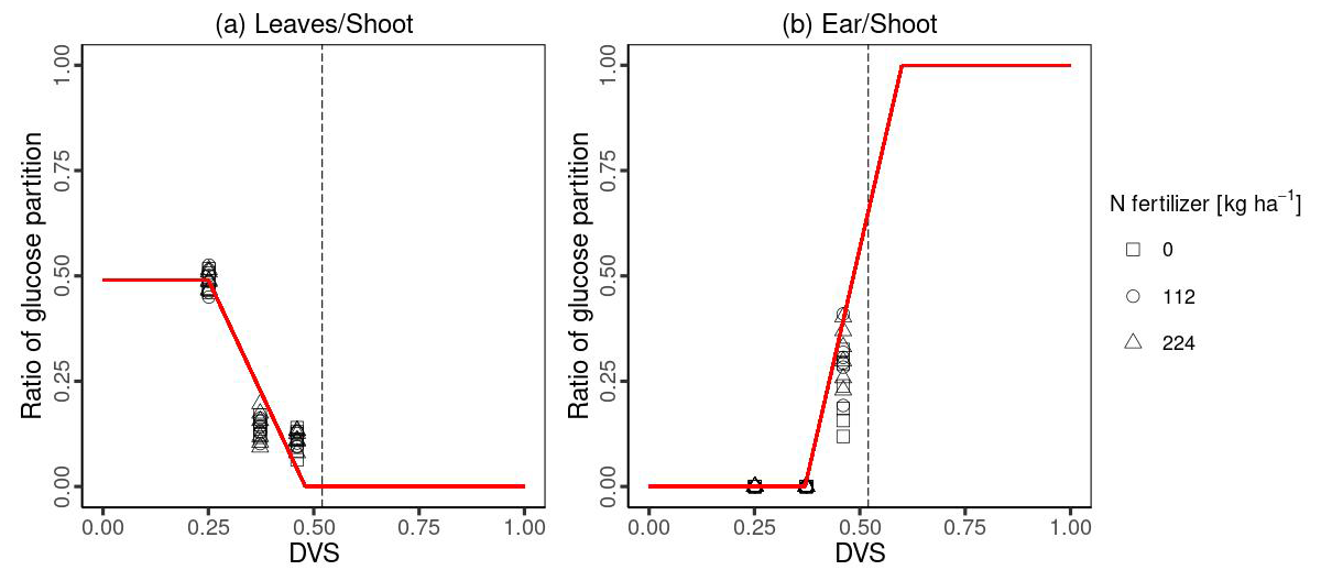
Figure 2 The ratio of glucose partitioning to leaves (a) and ears (b). Symbols show the ratio of glucose partition with different N_fert: 0 kg ha⁻¹ (square), 112 kg ha⁻¹ (cycle), and 224 kg ha⁻¹ (triangle) measured in Ciampitti et al. (2013a, b). The red lines in Fig. 2 show the segmented line parameters used in MATCRO-Maize, while the dashed line represents D_vs at flowering (D_vs,flw).

Specific leaf weight

The specific leaf weight (S_lw) is used to calculate the total leaf area index (L) in MATCRO. It is varied dynamically with the developmental stage of D_vs and is given by:

$$\begin{array}{}\text{(33)}& S_{\mathrm{lw}}=S_{\mathrm{lw},\mathrm{mx}}+\left(S_{\mathrm{lw},\mathrm{mn}}-S_{\mathrm{lw},\mathrm{mx}}\right)\exp (-k_{\mathrm{Slw}}{D}_{\mathrm{vs}})\end{array}$$

where S_lw,mn, S_lw,mx, and k_Slw are minimum, maximum, and absolute value of the rate constant in the S_lw function, respectively. These crop-specific parameters were derived from the observational data expressed in Table 1. We conducted curve fitting of S_lw to calculate the dry weight of the leaf biomass and the leaf area index based on Ciampitti et al. (2013a, b) and established a relationship (Fig. 3).

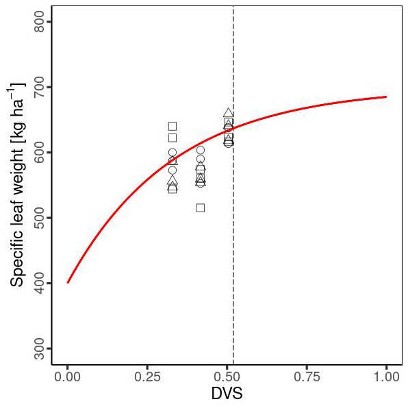
Figure 3 Relationships between specific leaf weights and developmental stages. Symbols are the same as in Fig. 2.

2.2.4 Crop height

Crop height (H_gt) is related to the calculation of evapotranspiration in MATCRO. It assumes that the dependence of the crop height is based on D_vs using function from Penning de Vries et al. (1989) and is given by

$$\begin{array}{}\text{(34)}& H_{gt}=\left\{\begin{array}{l}{h}_{aa}{D}_{\mathrm{vs}}/D_{\mathrm{vs},\mathrm{flw}},D_{\mathrm{vs}}<D_{\mathrm{vs},\mathrm{flw}}\\ h_{aa},D_{\mathrm{vs}}\ge D_{\mathrm{vs},\mathrm{flw}}\end{array}\right.\end{array}$$

where h_aa is the crop height at flowering (Table 1).

2.2.5 Crop yield

MATCRO calculates the final crop yield, Y_ld, from the dry weight of the storage organ at maturity (W_ear,mt) as follows:

$$\begin{array}{}\text{(35)}& Y_{\mathrm{ld}}=k_{\mathrm{yld}}{W}_{\mathrm{ear},\mathrm{mt}}.\end{array}$$

Here, k_yld is the crop-specific parameter (Table 1), which represents the ratio of Y_ld to W_ear,mt. The dry weight of the ear is a consistent predictor of the plant's potential yield at maturity. We parameterized K_yld using experimental data from Ciampitti et al. (2013b).

2.3 Model evaluation

MATCRO can run the simulation both at a point scale and at a global scale. The developed model was evaluated both at a point scale and at a global scale. For point scale levels, LAI and total aboveground were compared with the observation data from the four sites. Meanwhile, we use yield data for evaluation. After confirming the ability of the model to simulate maize growth, two types of evaluations were conducted at the global scale. First, the simulated yields at the grid cell were compared with the gridded yield datasets of the Global Dataset of Historical Yields (GDHY; Iizumi and Sakai, 2020), GlobalCropYield (GCY; Cao et al., 2025), and the Spatial Production Allocation Model (SPAM; IFPRI, 2019). Second, the simulated yields at the country and total global levels were compared with the country yield report and global data from the Food and Agriculture Organization's FAOSTAT database (FAOSTAT, 2024). To quantify the model performance, four statistical values were used in this study: the Pearson correlation coefficient (COR), root mean square error (RMSE), relative root mean square error (RRMSE) and normalized mean absolute error (NMAE). RRMSE and NMAE were calculated as follows:

$$\begin{array}{}\text{(36)}& {\displaystyle }\mathrm{RMSE}=\sqrt{{\displaystyle \frac{\mathrm{1}}{n}}{\sum }_{i=\mathrm{1}}^n{\left(y_i-{\widehat{y}}_i\right)}^{\mathrm{2}}},\text{(37)}& {\displaystyle }\mathrm{RRMSE}={\displaystyle \frac{\mathrm{RMSE}}{\stackrel{\mathrm{‾}}{y}}},\text{(38)}& {\displaystyle }\mathrm{NMAE}={\displaystyle \frac{\mathrm{1}}{n}}{\sum }_{i=\mathrm{1}}^n{\displaystyle \frac{\left|{\widehat{y}}_i-y_i\right|}{y_i}},\end{array}$$

where y_i is the actual value, ${\widehat{y}}_i$ is the predicted value, and $\stackrel{\mathrm{‾}}{y}$ is the mean of the actual value.

2.3.1 Model evaluation at a point scale

To evaluate the model performance at a field scale, we used observational data from four sites (Brazil, France, Tanzania, and the USA; Table 2) used in the Agricultural Model Intercomparison and Improvement Project (AgMIP) study (Bassu et al., 2014). We used local daily climate data of precipitation, downwards shortwave radiation, air temperature, wind speed (P_rc, R_s, T_a, U respectively), management data (N_fert and irrigation regime) and phenological data (planting, flowering, and maturity dates) for model input data at each site. We identified the soil texture from the gridded soil texture dataset of ISIMIP (Volkholz and Müller, 2020), and annual CO₂ data from the ISIMIP3a (Büchner and Reyer, 2022). Climatic data were obtained from the NASA Modern Era Retrospective-Analysis for Research and Applications corrected with observational datasets (AgMERRA; Ruane et al., 2015) when measured data were unavailable (Bassu et al., 2014).

Table 2 Evaluation site information in the point-scale simulation.

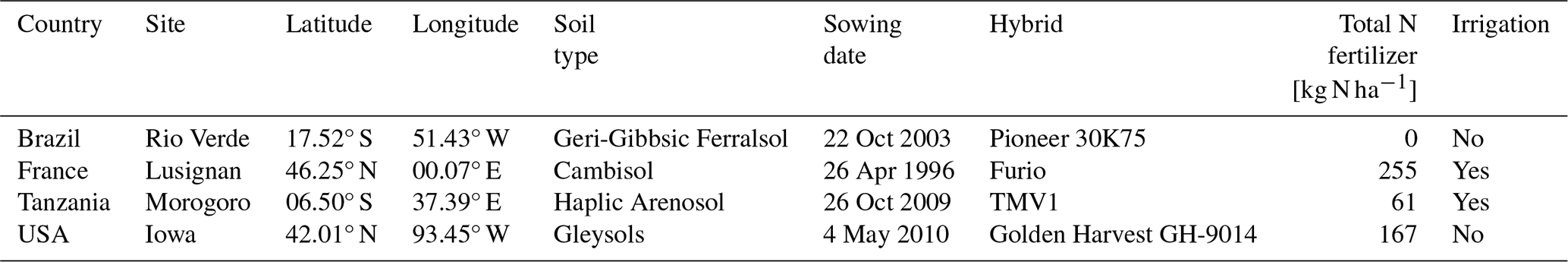
Notably, air pressure (P_s) and specific humidity (S_h) data were not provided. Hence, we represented the point scale by extracting P_s from the nearest 0.5° × 0.5° grid cell of GSWP3-W5E5 dataset for the ISIMIP3a (Lange et al., 2022). Meanwhile, S_h was converted from R_h using T_a and the vapour pressure. We parameterized G_dd,m and D_vs,flw based on T_a and phenological data (sowing, flowering, and maturity dates). G_dd,m calibrated for each site is used for the simulations, while the average D_vs,flw over the 4 sites is used (0.52 in Table 1). As a result, the mean average errors were estimated as 4.25 and 7 d for flowering and maturity, respectively (Fig. 4). MATCRO was run with these parameters, and then the model output was evaluated with the observations for the following 3 variables: seasonal change in the LAI, total aboveground biomass, and final yield.

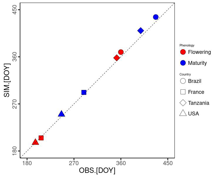
Figure 4 Model-fit comparison of the flowering and maturity date simulations (SIM on the y axis) and observations (OBS on the x axis). DOY represents the number of days from 1 January. Symbols show each site: Brazil (square), France (circle), Tanzania (triangle), and the USA (diamond). The colours indicate the phenological stages of flowering (red) and maturity (blue).

Model calibration was conducted based on phenological data (Table 2, Bassu et al., 2014) and biomass data for carbon partitioning of leaves and ear (Fig. 2, derived from Ciampitti et al., 2013a, b). In this study, a global parameter was applied uniformly across all regions at the grid-cell level instead of using site-specific calibrated parameters in the simulations. The model was then assessed at the point scale to verify calibration for phenology (flowering and maturity) and was evaluated against time-series data of LAI, aboveground biomass, and harvested yield (see Sect. 3.1), which were not included in the model calibration.

2.3.2 Model evaluation at a global scale

Simulation settings

For the global-scale simulation, the model was run at a spatial resolution of 0.5° × 0.5° from 1980–2010 under both rainfed and irrigated conditions. The required input data were as follows: (i) crop calendar data were from the Global Gridded Crop Model Intercomparison (GGCMI) phase 3 protocol (Jägermeyr et al., 2021). It provides planting and maturity dates for 18 different crops, including maize, separated by rainfed and irrigated systems. We parameterized the average G_dd,m at each grid over the period 1980–2010 for the growing season from the planting to maturity dates for each of the rainfed and irrigated conditions. Both the planting date and the simulated G_dd,m were used as the input data for the global-scale simulations. (ii) Water management data (i.e., irrigation regime) from the MIRCA2000 dataset (Portmann et al., 2010). In the case of irrigated conditions, the soil moisture was set to field capacity during the growing season. (iii) N_fert from the Inter-Sectoral Impact Model Intercomparison Project (ISIMIP; Volkholz and Ostberg, 2022). It provides the annual nitrogen fertilizer inputs for five crop types, including C₄ annual crops for maize. (iv) Soil texture classification from ISIMIP3a protocol soil input data (Volkholz and Müller, 2020). (v) Annual atmospheric CO₂ data from the ISIMIP3a (Büchner and Reyer, 2022). (vi) Six types of daily meteorological for model inputs (P_s, P_rc, R_s, S_h, T_max, T_min, T_a, U) from the GSWP3-W5E5 dataset for the ISIMIP3a dataset (Lange et al., 2022). We set the data from (i), (ii), and (iv) as constants across the simulation period, whereas the data from (iii), (v), and (vi) are variables.

Analysis

MATCRO-Maize was first assessed for the phenological simulation of harvest time against the GGCMI dataset (Jägermeyr et al., 2021) and global datasets of crop phenological events for agricultural and earth system modeling (GCPE), which were derived from various field experiments and a phenology model (Mori et al., 2023). These datasets were compared under both rainfed and irrigated conditions at a 0.5° × 0.5° resolution to check the model's performance. Then, we assessed the yields by combining simulated yield at irrigated and rainfed according to the maize area in each grid cell.

The simulated final yields in each grid cell under irrigated and rainfed conditions were aggregated by grid cell, country and global level with the harvested area from MIRCA2000 data (Portmann et al., 2010) via the following equation for each year from 1981–2010:

$$\begin{array}{}\text{(39)}& \begin{array}{rl}& {\mathrm{Yield}}_{\mathrm{aggregated}}=\\ & {\displaystyle \frac{{\sum }_{i=\mathrm{1}}^n\left({\mathrm{Yield}}_{i,\mathrm{rf}}\times {\mathrm{Area}}_{i,\mathrm{rf}}\right)+{\sum }_{i=\mathrm{1}}^n\left({\mathrm{Yield}}_{i,\mathrm{irr}}\times {\mathrm{Area}}_{i,\mathrm{irr}}\right)}{{\sum }_{i=\mathrm{1}}^n\left({\mathrm{Area}}_{i,\mathrm{rf}}+{\mathrm{Area}}_{i,\mathrm{irr}}\right)}}\end{array}\end{array}$$

where Yield_aggregated is the aggregated yield with the total grid cells (n) in grid cell i. Yield_rf and Yield_irr are the simulated yields under rainfed and irrigated conditions, respectively, and Area_rf and Area_irr are the harvested areas from MIRCA2000 for rainfed and irrigated conditions, respectively.

The model performance was evaluated by comparing its output with the historical yield dataset. The grid-cell-level yield was averaged across a 30-year period (1980–2010) and compared with the Global Dataset of Historical Yields (GDHY; Iizumi and Sakai, 2020) for 1980–2010, an upscaled GlobalCropYield dataset with 5 min resolution (GCY; Cao et al., 2025) for 1981–2010, and the Spatial Production Allocation Model (SPAM; IFPRI, 2019) for the year 2020. The country and global-level yields were compared with FAOSTAT data (FAOSTAT, 2024) for the average and annual variabilities over the 30 years. In the comparison at the country level, we focus on the top 20 maize-producing countries that account for more than 85 % of total maize production.

We focused on two perspectives for evaluation: (i) the ability of the model to capture the spatial distribution of yield in both low and high-producing countries and (ii) the ability of the model to reproduce the climatic effect reflected in the interannual variability at the country and global scales. The first perspective was analysed using NMAE to quantify model error for both the global yield and the yield of the top 20 producing countries. The 30-year average yields were also compared based on the statistics of COR, RMSE, and RRMSE to confirm accuracy. The second perspective was analysed via the COR of the detrended deviation between the simulated and FAOSTAT yields to assess the interannual variability.

3 Results

3.1 Point-scale simulations

A comparison of the time series changes in the LAI at each experimental site is shown in Fig. 5. In general, MATCRO-Maize captured the increasing trend towards flowering time, followed by a decreasing trend towards the end of maturity. Especially during the vegetative stage ($D_{\mathrm{vs}}<D_{\mathrm{vs},\mathrm{flw}}:\mathrm{0.52}$), the simulated LAI showed relatively good agreement. However, the simulated LAI was notably underestimated in Brazil and France immediately before the reproductive stage (near the dashed black line in Fig. 5). The LAI underestimation in France and Brazil (Fig. 5) could also be seen with a large RMSE, which is approximately 50 % of the average LAI across all observational values at 3 sites except for Tanzania during the crop growth, although overall, the comparison was statistically significant (p value < 0.01), with a COR of 0.762.

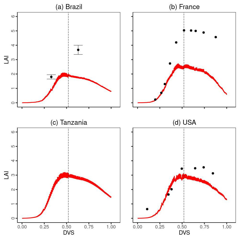
Figure 5 Temporal evaluation of leaf area index (LAI) simulated by MATCRO-Maize (red line) at each site: (a) Brazil, (b) France, (c) Tanzania and (d) the USA across the developmental stage (D_vs). The observation data in each site are shown by black points. Notably, there were no observational data in Tanzania. The error bars were provided only for Brazil. The dashed black line shows the flowering time.

Figure 6 compares the time series of total aboveground biomass between the simulated and experimental data. Except for Tanzania, MATCRO-Maize accurately estimated the increasing trend of total aboveground biomass towards maturity (Fig. 6a and b), although the simulated biomass in Brazil was underestimated at maturity (Fig. 6a). The simulated total aboveground biomass in Tanzania increased until maturity, while the observations gradually decreased towards the maturity time (Fig. 6c). The comparison of total aboveground biomass during the crop growth was statistically significant (p value < 0.001), with a COR of 0.895, although the RMSE was 3628.3 [kg ha⁻¹], which corresponds to approximately 35 % of the average of all observed total aboveground biomass.

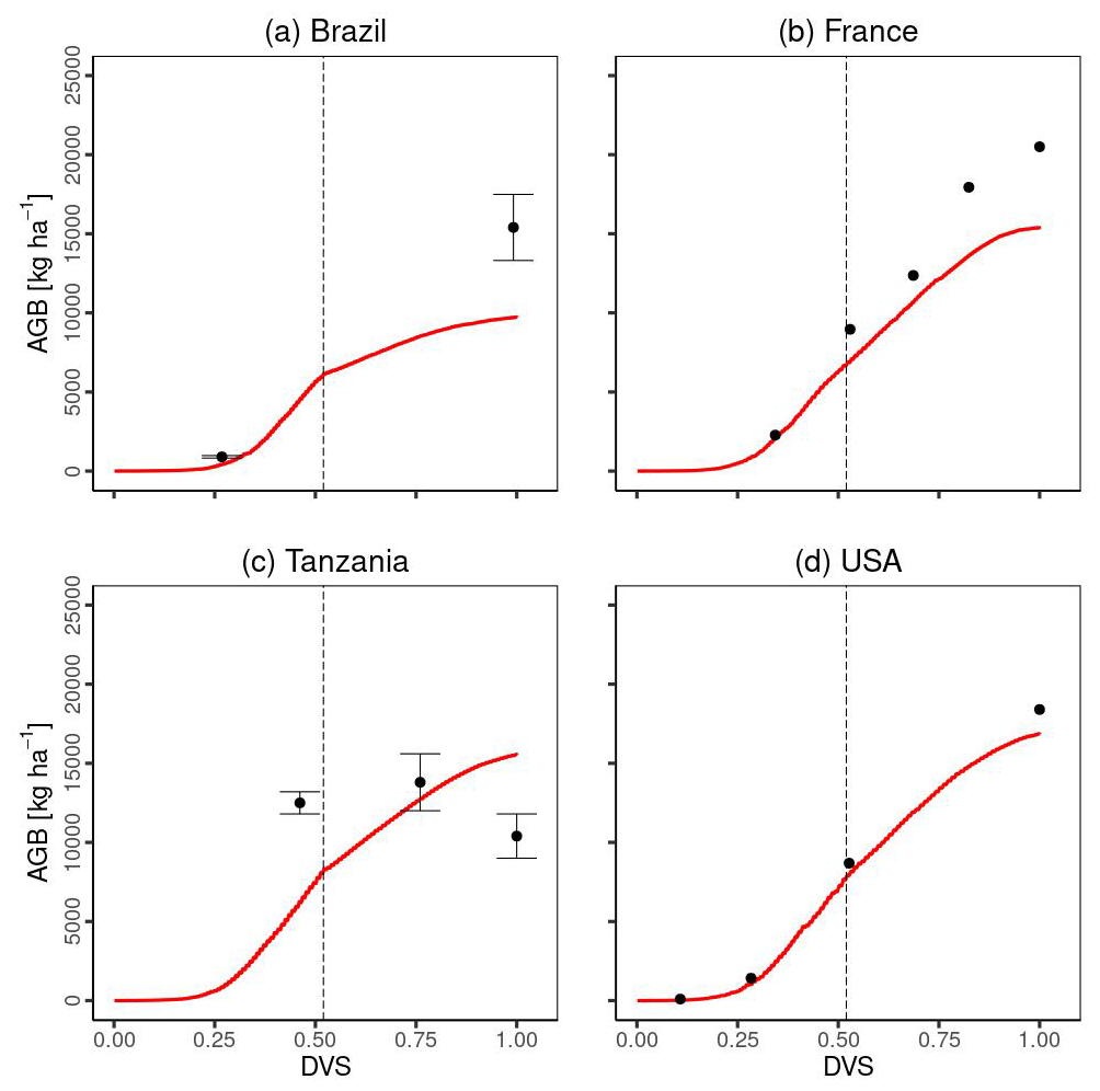
Figure 6 Temporal evaluation of total aboveground biomass (AGB) simulated by MATCRO-Maize (red line) at each site: (a) Brazil, (b) France, (c) Tanzania and (d) the USA across the developmental stage (D_vs). The observation data in each site are shown by black points. The error bars were only provided for Brazil and Tanzania. The dashed black line shows the flowering time.

Figure 7 compares the 1:1 line between the simulated and experimental data for harvested yield. The comparison of the final crop yield was statistically significant (p value < 0.01). It had a relatively low COR compared with the LAI and total aboveground biomass, due to the small sample size (N= 4) and the overestimation for Tanzania. The RMSE was 2575.0 [kg ha⁻¹], which is approximately 30 % of the average observational yield at all the sites. It is noted that Figs. 5–7 present the model evaluation using independent data. Evaluation was performed using a global parameter from the literature to simulate the plant organs in the global-scale simulation, which may have resulted in some deviations.

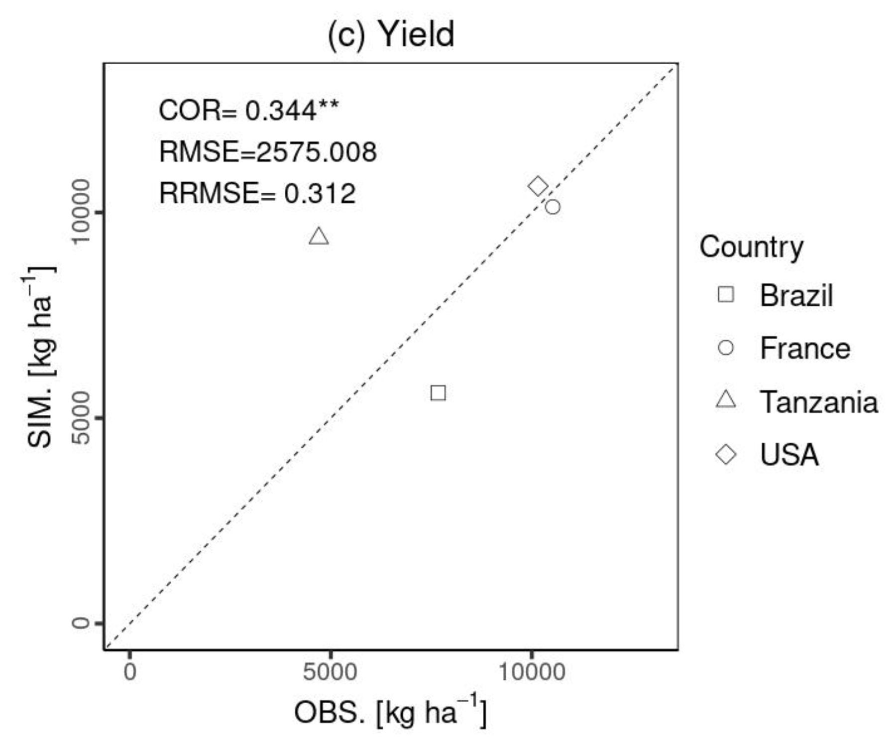
Figure 7 Statistical comparison (COR, RMSE, and RRMSE) of maize yield. The x axis (OBS) represents the observational data, and the y axis (SIM.) is the simulated data. Shapes show each site: Brazil (square), France (circle), Tanzania (triangle), and the USA (diamond). Notably, there was no observed LAI in Tanzania. The symbols ${}^{***}$, ${}^{**}$, indicate p values < 0.001 and 0.01, respectively.

3.2 Global-scale simulations

3.2.1 Phenology

The timing of seasonal biological events (i.e. harvest time) has a significant impact on crop growth and yield outcomes. Global yield is affected by global phenology. We assessed agreement to check the model performance by comparing the difference between simulated global average harvest time (1981–2010) with the gridded global dataset of phenological datasets of GGCMI (Fig. 8a and b) and GCPE (Fig. 8c and d). The maps show consistent spatial patterns for later harvest time between the simulation and the reference datasets, in parts of Brazil, USA, southern and central Africa. The discrepancies between datasets are likely produced due to the difference in phenology parameterization and management assumptions where GGCMI and GCPE used different methodologies and data sources. Moreover, the use of the average growing degree day in the simulations led to year-to-year differences in harvest time compared with the reference crop calendar used for the input data (Fig. 8a and b). The mean absolute differences in harvest time (Fig. 8e and f) indicate that the largest biases occur mostly in tropical regions.

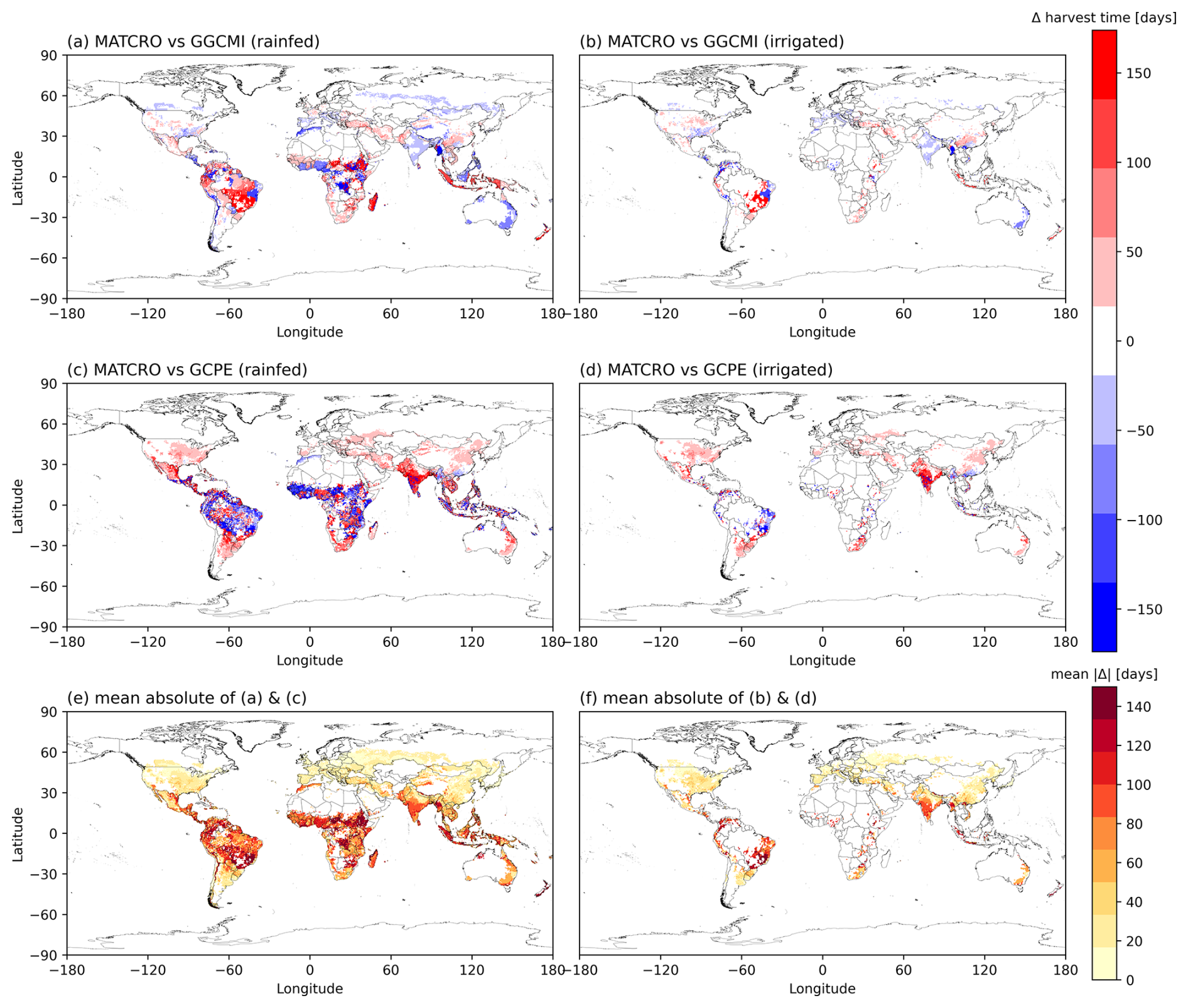
Figure 8 The difference between simulated harvest time (days) in MATCRO-Maize simulations with: (a) GGCMI in the rainfed, and (b) irrigated conditions; (c) GCPE in the irrigated, and (d) rainfed conditions. Blue indicates underestimation, while red indicates overestimation between simulations and references. Panels (e) and (f) show the mean of absolute differences (days) between simulations and two reference datasets under the rainfed (a, c) and irrigated (b, d) conditions, respectively.

3.2.2 Yield

A comparison of the global distributions is shown in Fig. 9 (simulations: Fig. 9a; observation datasets: Fig. 9b, c, and d). All datasets were harmonized to a 0.5° × 0.5° resolution, including simulated yield from MATCRO-Maize (Fig. 9a), GDHY (Fig. 9b), GCY (Fig. 9c), and SPAM (Fig. 9d). The data were averaged over 30 years (1981–2010) for GDHY, over 29 years (1982–2010) for GCY, and at the year 2010 for SPAM. While the overestimation is mainly evident in tropical regions, the simulated yield could capture high-yielding regions, including the Corn Belt in the United States and the northern part of China, in agreement with the reference datasets.

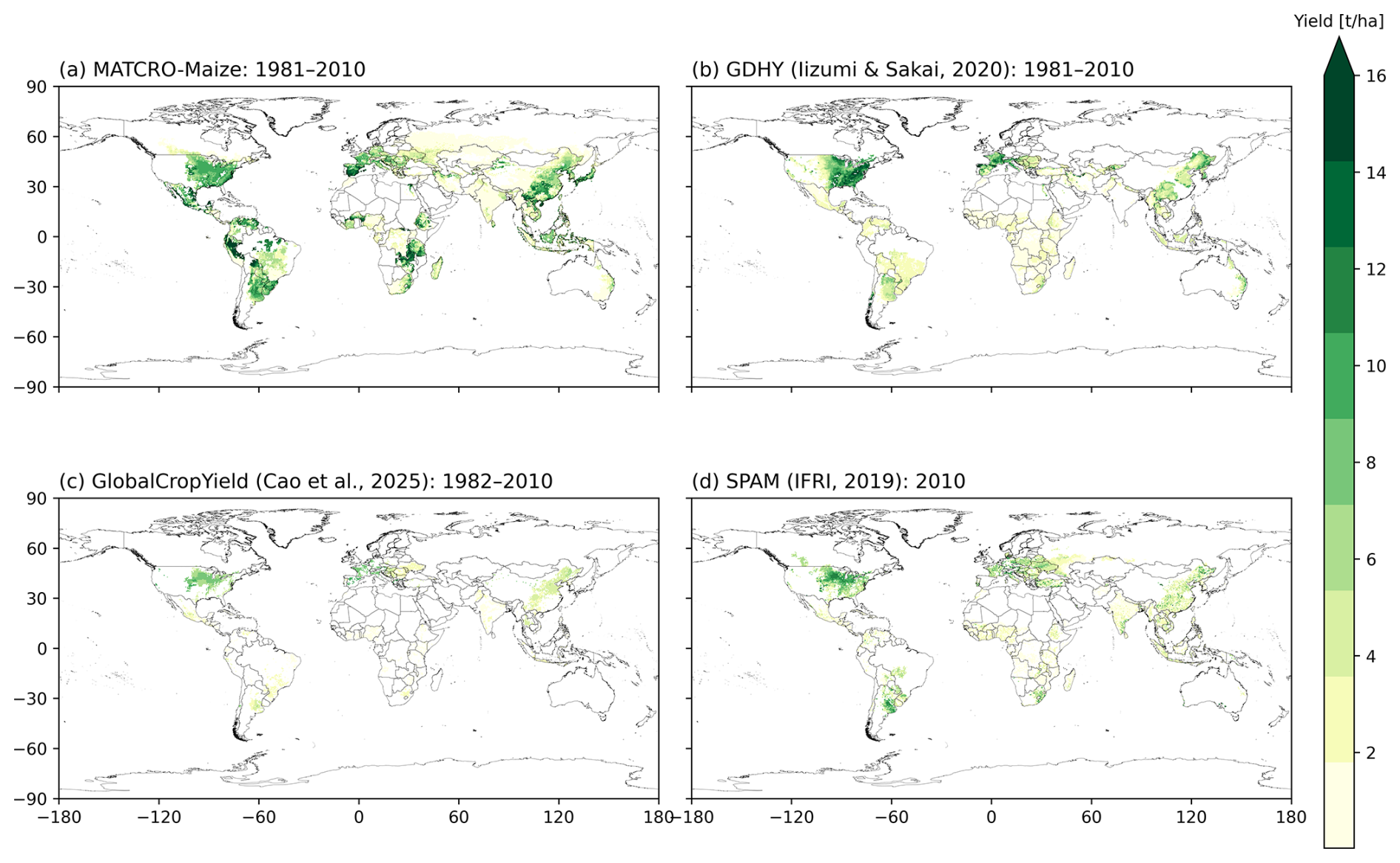
Figure 9 Global distribution of the 30-year average (1981–2010) maize yield by (a) simulations from the MATCRO-Maize and (b) the GDHY dataset. For comparison, yield estimates from shorter periods are also shown from (c) GCY for 29-year average (1982–2010) and (d) SPAM2010 for year 2010. The yield is aggregated based on the harvested area from MIRCA2000.

Temporal changes in the global yield across 30 years indicated that the simulated global yield had an NMAE of 0.67. This shows a simulation error of 67 % with respect to the average FAOSTAT yield. The comparison of interannual variability between the simulations and observations was statistically significant (p value < 0.01), with a COR of 0.549 (Fig. 10). For the top 20 producing countries, MATCRO-Maize also tended to overestimate the annual yield (Fig. 11) and the average yield over a 30-year period (Fig. 12). The overestimation was particularly pronounced in Egypt, where the simulated yield was approximately four times greater over a 30-year period. In terms of interannual variability, half of the 20 countries showed statistically significant correlations: six countries had p values < 0.001, two countries had p values < 0.01, and two countries had p values < 0.05 (Fig. 11). The 30-year average comparison was also statistically significant (p value < 0.01), with a COR of 0.58, although the RMSE was 4007.7 [kg ha⁻¹] (Fig. 12).

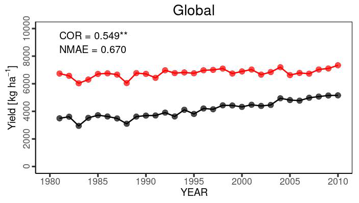
Figure 10 Interannual variability in global maize yield from 1981 to 2010 for our simulation (red circles) and FAOSTAT (black) yields. COR represents the correlation coefficient of interannual variability. NMAE means normalized mean absolute error. Asterisks ${}^{**}$ indicate p value < 0.01.

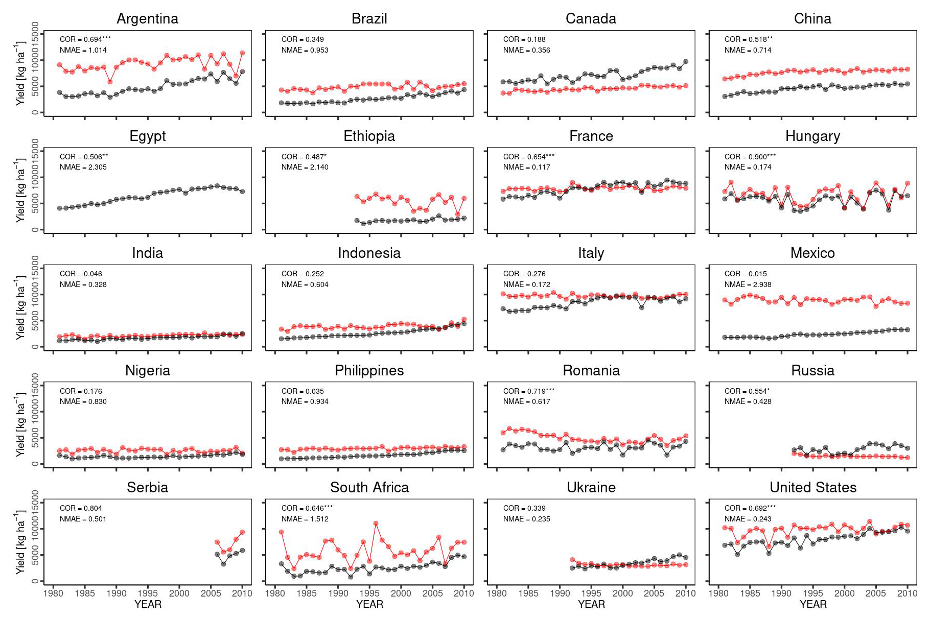
Figure 11 Comparison of interannual variability for the top 20 maize-producing countries. Similar to Fig. 9. Notably, the simulated yield in Egypt is not shown as it extends beyond the range of the y axis. The symbols ${}^{***}$, ${}^{**}$, and ^* indicate p values < 0.001, 0.01, and 0.05, respectively.

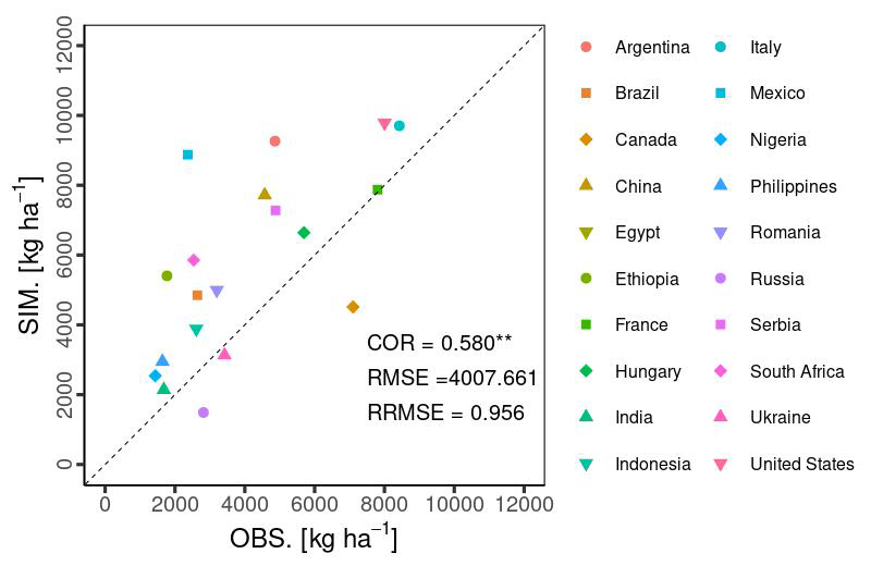
Figure 12 Accuracy of the 30-year average of the simulated yield (SIM) to the observed yield (OBS from FAOSTAT data) for the top 20 countries. Symbols show the average yield in each country. Notably, the Egypt data points are not shown as exceeding the range of the y axis. Asterisks ${}^{**}$ indicate a p value < 0.01.

3.3 The effects of photosynthesis and N fertilizer

In addition to the yield comparison, we analysed the effect of nitrogen fertilizer (N_fert) on maize yield, as it is a key determinant of crop yield. It compared both simulated yield data and FAOSTAT yield data with N_fert for a 30-year average using a fitted polynomial curve (quadratic polynomial regression). We also conducted two tests to quantify the effects of the N_fert-related function and parameters as follows: (i) Eq. (27) during the vegetative stage is derived from Drouet and Bonhomme (2004), defined as “test S_ln-V_cmax”, where V_cmax(0) used this function:

$$\begin{array}{}\text{(40)}& \begin{array}{rl}{V}_{\mathrm{cmax}}\left(\mathrm{0}\right)& =\mathrm{36.8}\times \left\{{\displaystyle \frac{\mathrm{2}}{\mathrm{1}+\exp \left[-\mathrm{2.45}\cdot \left(S_{\ln }-\mathrm{0.27}\right)\right]}}-\mathrm{1}\right\},\\ & D_{\mathrm{vs}}<D_{\mathrm{vs},\mathrm{flw}}\end{array}\end{array}$$

and (ii) S_ln,plt used parameter value from 0.825 (Table 1) to 0.5 (defined as “test S_ln,plt”).

Figure 13 illustrates the comparison of country-level yield data with nitrogen fertilizer levels: (a) FAOSTAT data, (b) simulated yield by MATCRO-Maize, (c) the impact of reduced Rubisco activity on photosynthetic rates based on experimental data from Drouet and Bonhomme (2004) in the “test Sln-Vcmax” scenario, and (d) the effect of reduced photosynthetic rates due to lower initial specific leaf nitrogen at planting time in the “test Sln,plt” scenario. The nitrogen fertilizer values were derived from the gridded dataset of N fertilizer from ISIMIP (Volkholz and Ostberg, 2022).

Figure 13a and b show the comparisons based on N_fert for each FAOSTAT and simulated yield, respectively. MATCRO has a strong N_fert effect on the yield reflected in the steep upward trend of the fitted curves. This effect was scarcely alleviated by the intentionally reduced effect of photosynthesis (Fig. 13c and d), mainly because of the effect of Egypt as an outlier with higher values. Without Egypt as an outlier, the curves for FAOSTAT and MATCRO-Maize were more comparable. The maize yield in Egypt shows high value compared to other countries where significant overestimation was observed.

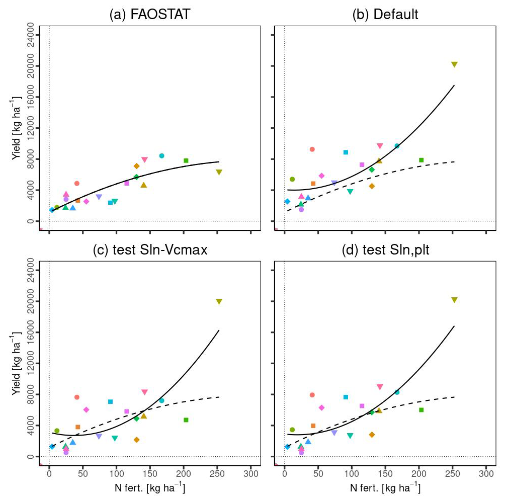
Figure 13 Relationship between N_fert and yield in (a) FAOSTAT data, (b) simulated yield with the original setting (Default), (c) simulated yield with the changed S_ln−V_cmax relationship (test Sln-Vcmax), (d) simulated yield with the changed parameter related to the D_vs−S_ln function (test Sln, plt). N_fert (N fertilizer) and country yield were averaged across 30 years for each country. The legends for symbols are the same as those in Fig. 11. The solid lines are the fitted curves for the data, while the dashed line in (b), (c), and (d) indicates a fitted curve in (a). All lines were fitted using a quadratic polynomial regression.

4 Discussion

4.1 Point-scale simulations

The point-scale simulations were evaluated using global parameters to assess their ability to capture broad yield patterns across different regions. The simulated harvested yield showed statistically significant correlations at the point scale (Fig. 7), indicating that the MATCRO-Maize model could simulate maize growth and yield. However, there were some discrepancies between the simulations and observations that remain due to the limitations of using global parameters, such as the underestimation of the LAI in Brazil and France, the underestimation of the total aboveground biomass in Brazil, and the different growth trends of the total aboveground biomass in Tanzania. The underestimation of LAI is primarily due to the use of global morphological parameters at the site scale. Further investigation will improve site-specific performance by coupling LAI to key soil properties (soil organic carbon, total nitrogen, and water-holding capacity) and by incorporating canopy cover fraction following Hasegawa et al. (2008). Global parameters at the point scale enable testing the model's applicability across various regions, although local variations in soil, climate, or crop management may not be fully captured in this study.

One potential factor contributing to the underestimation of the LAI in France might be related to the effect of plant density, which is not currently considered in MATCRO. The actual plant density [plants m⁻²] at each site was 9.5 (France), 7.5 (USA), 6.6 (Brazil), and 9.5 (Tanzania) (Bassu et al., 2014). Some studies have shown that LAI trends are affected primarily by the plant density factor relative to N_fert and hybrids (Boomsma et al., 2009; Ciampitti et al., 2013a; Ciampitti and Vyn, 2011). MATCRO could not reproduce the trends driven by plant density leading to underestimation, although other important factors (e.g., management practices, climatic conditions), which are quite different from each site in the literature, would also affect crop growth variables, including the LAI.

Both the underestimation of the LAI and total aboveground biomass in Brazil were caused by the field experimental conditions of N_fert=0, given its effect on crop growth in MATCRO. The reason for the lack of fertilization in the field experiment was that sufficient N was released by organic matter mineralization (Bassu et al., 2014), which was not considered in the model. Moreover, N_fert directly affects S_ln in MATCRO, with an increasing trend towards flowering and then a decreasing trend towards maturity (Fig. 1). S_ln is related to V_cmax25(0), which in turn affects the photosynthesis calculation (Sect. 2.1 and 2.2.2). In particular, during the reproductive stage, we used Eq. (27), which results in a low V_cmax25(0) under low S_ln due to the more gradual slope of the curve compared with the vegetative stage (1.41 for the reproductive stage and 2.9 for the vegetative stage, in Eq. 27). The lower photosynthesis rate indirectly affected low biomass accumulation in Brazil. This could be attributed to the underestimation of total aboveground biomass at maturity (Fig. 6a).

For underestimation of the LAI, low leaf biomass accumulation, which is derived from the same mechanism, would be the reason considering the calculation process of the LAI in MATCRO. The LAI is determined by the division of the leaf biomass weight by S_lw, which depends on D_vs. Because S_lw is calculated from the same parameter at all sites (Eq. 33) and Fig. 3), leaf weight is the factor that causes differences between sites, leading to the underestimation of the LAI in Brazil. Therefore, the condition of N_fert=0 might be the reason for both underestimations.

Another reason for the difference in the growth trend of biomass in Tanzania was related to the length of the growing season. The cultivar used in Tanzania was a short-season type with 99 d of observed growing season length, whereas the cultivars at other sites were medium- or long-season types with lengths ranging from 122 to 173 d (Bassu et al., 2014). Capristo et al. (2007) reported that, compared with medium- and long-season cultivars, short-season cultivars presented the lowest biomass accumulation from flowering to maturity, which was reflected in the observed biomass (Fig. 6c). This suggests that the trend of biomass accumulation varies across growing season types. Although other factors, such as climatic conditions or biotic stresses, could also affect the biomass accumulation. While MATCRO considers the growing season length as G_dd,m to judge the harvesting time, this does not mean that MATCRO could capture the difference in trends due to growing season types, leading to the gap between the simulations and observations shown in Tanzania.

4.2 Global-scale simulations

A comparison of the global distribution of maize yield revealed that MATCRO-Maize could capture the distribution of high-yield regions but could not capture the yield in tropical regions (Figs. 8 and 9). Similar overestimations in tropical regions have also been reported in other global models, possibly because of the lack of representation of extreme weather events or crop pests (Lombardozzi et al., 2020; Osborne et al., 2015). Moreover, soil fertility is also an important source of model error and contributes to spatial variation.

Notably, MATCRO-Maize tended to overestimate the absolute values for global yield and the yields of the top 20 countries, as reflected in the NMAE and RMSE values (Figs. 10, 11, and 12). The simulated total global yield is mainly determined by the yields of the top three maize-producing countries: the United States, China, and Brazil, which have large cultivation areas (Table 3). The yields of all three countries were overestimated, with simulated yields approximately 1.2, 1.7, and 1.8 times greater than the 30-year averages of the observed values in the United States, China, and Brazil, respectively, leading to an overestimation of the total global yield. Such overestimations in the main producing countries, especially in China and Brazil, are also observed in other global crop models (von Bloh et al., 2018; Osborne et al., 2015; Schaphoff et al., 2018). This indicates that there are important factors for determining yields that are not considered in most crop models.

Table 3 Maize cultivated land area for 20 major producer countries from MIRCA2000 (Portmann et al., 2010).

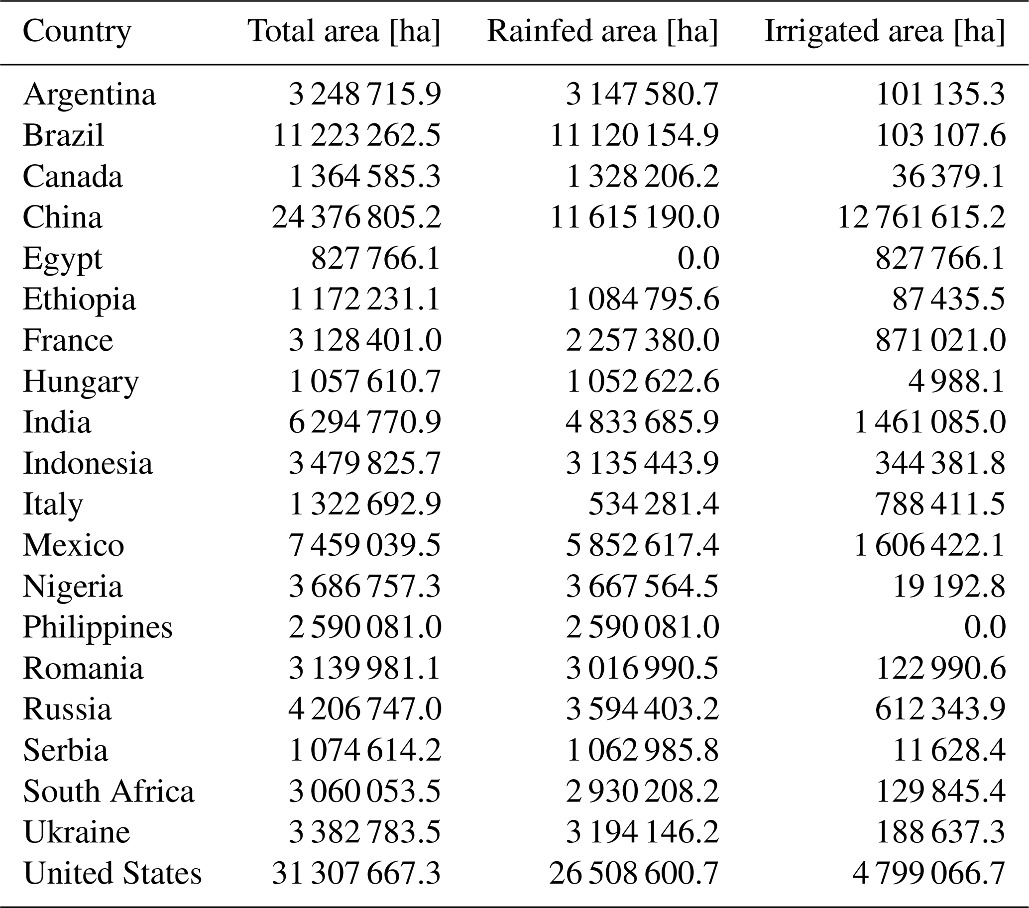
For the top 20 producing countries, the overestimation was particularly strong in Egypt, with a simulated yield approximately four times greater than that reported by FAOSTAT. This overestimation is caused by the irrigated conditions in all grids in Egypt. Under simulation in rainfed conditions, crop growth in Egypt was not simulated in the model due to the inhibited photosynthesis rate caused by strong water stress. Under irrigated conditions, this strong water stress was alleviated. In addition, the radiation in Egypt was consistently strong throughout the growing period, and N_fert was highest among the top 20 countries across the 30-year simulation. The reported N_fert increased from approximately 180 kg ha⁻¹ in 1980 to 360 kg ha⁻¹ in 2010. This caused the photosynthesis rate to be high (Eq. 4) across the growing seasons, leading to marked overestimation.

The current version of MATCRO-Maize can reproduce yield responses to nitrogen fertilization across a range of fertilizer levels, but it tends to overestimate yields under certain conditions (e.g., Egypt). This occurs because the model assumes high nitrogen use efficiency and idealized irrigation conditions, where actual yields are constrained by soil quality, management, and local cultivar traits not explicitly represented. This suggests that the representation of nitrogen effects in the model remains simplified, and further refinement is needed for region-specific scale simulation.

Although the simulated yield has the large error in terms of the absolute value, the comparison of the 30-year average yield was statistically significant, with a COR of 0.58 (p value < 0.01) and an RMSE of 4008 kg ha⁻¹ (Fig. 12), showing the ability to capture the spatial distribution of the yield both in low- and high-producing countries from the first perspective of the comparison (Sect. 2.3.2). This result was comparable to another model, LPJ-GUESS (Olin et al., 2015), with a COR of 0.46 and an RMSE of 4300 kg ha⁻¹ (Table 4). However, the targeted countries differed in scope (top 20 producing countries for MATCRO-Maize, and whole countries for LPJ-GUESS).

In terms of interannual variability from the second perspective, the total global yield and approximately one-third of the top 20 producing countries were statistically significant, with p values < 0.01 (Figs. 10 and 11). It indicates that MATCRO-Maize could reproduce the climatic effect globally to some extent. This result is also supported by similar comparisons of other global crop models in terms of statistics (Table 4). However, it is difficult to simply compare the statistical values between the models owing to the differences in periods, input data, and methods for detrending and aggregating the yield. The COR of interannual variability for total global yield in MATCRO-Maize was in the range of those of the other models (0.55; 0.42–0.89, respectively). For the top 20 countries, almost all the COR values also fell within the range of the other models. Therefore, these comparisons from two perspectives might indicate that MATCRO-Maize reproduces reasonable results. The moderate correlations observed reflect the typical influence of yield data variability and uncertainty in management practices across regions.

Table 4 Statics of model simulation accuracy of the MATCRO-Maize and other crop models. Notably, the asterisks for GGCMI phase I indicate the p values: ${}^{***}$ for p values < 0.001, ${}^{**}$ for p values < 0.05, ^* for p values < 0.1, whereas those of LPJmL4 and MATCRO-Maize indicate the p values: ${}^{***}$ for p values < 0.001, ${}^{**}$ for p values < 0.01, ^* for p values < 0.05.

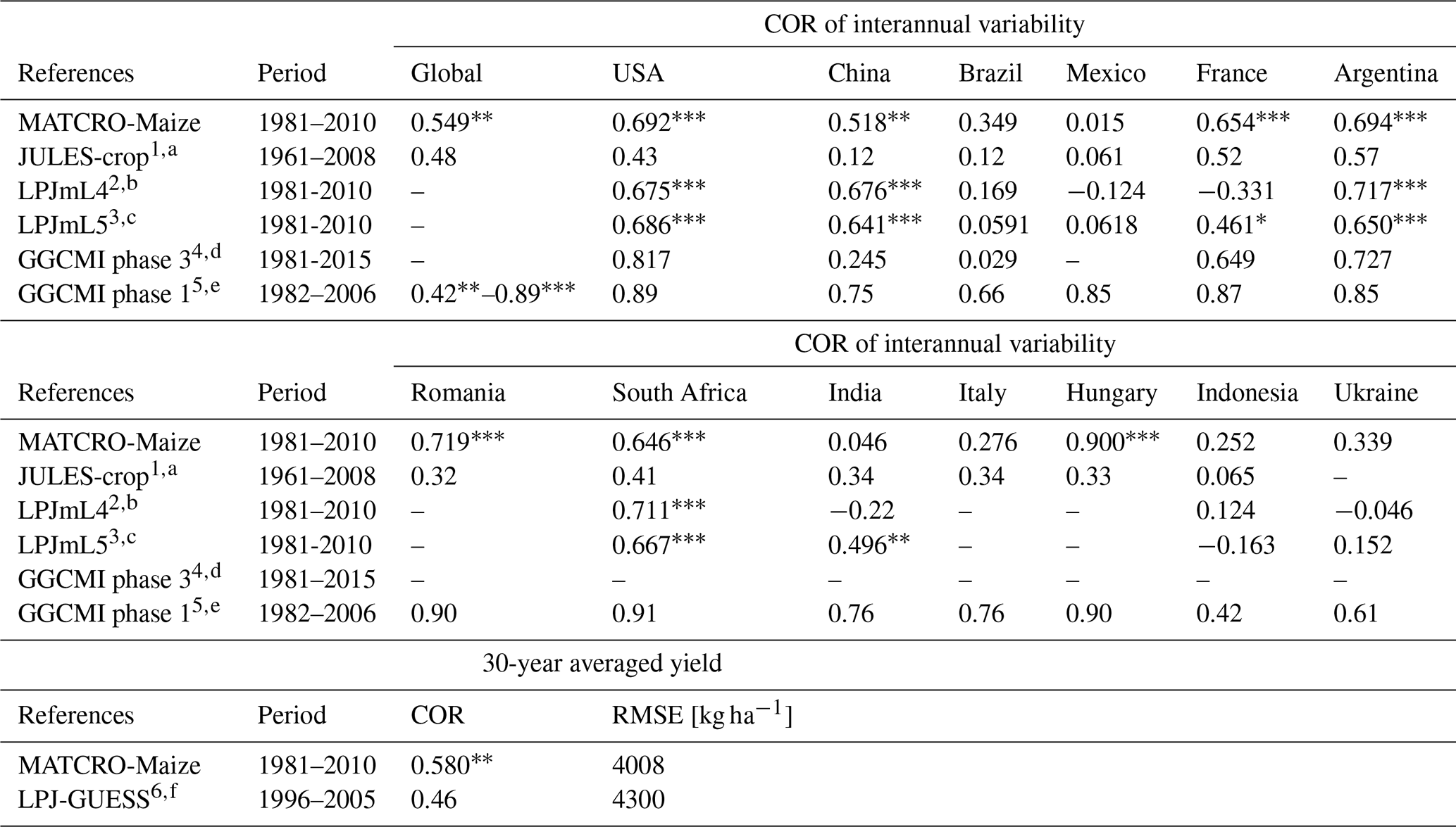
¹ Countries-level comparison was conducted for 12 countries, which were detrended only for observation. p values are not shown. ^2,3 Countries-level comparison was conducted for the top 10 producing countries, which were detrended via a 5-year moving average. ⁴ Twelve global gridded crop models were used. The COR shown here is the ensembled mean value for the 5 largest producing countries after detrending. p values are not shown. ⁵ Fourteen global gridded crop models were used. The COR of the global yield shown here is the minimum and maximum value, except for one nonsignificant correlation with the default setting. The COR of each country shown here is the best correlation among the 14 models, including 3 different settings with statistical significance (p values are not shown). For both the global and country-level comparisons, a 5-year moving average was used to remove trends. ⁶ The 10-year average comparisons included all countries. p values are not shown. ^a Osborne et al. (2015), ^b Schaphoff et al. (2018), ^c von Bloh et al. (2018), ^d Jägermeyr et al. (2021), ^e Müller et al. (2017), ^f Olin et al. (2015).

4.3 Model limitations

MATCRO-Maize currently lacks explicit simulation of soil organic carbon and soil nitrogen mineralization. Instead, the effects of nitrogen supply are represented by describing the relationship between a broad range of nitrogen fertilization levels (Muchow, 1988) and specific leaf nitrogen (SLN), which subsequently affects photosynthetic capacity (Vcmax). While this simplification allows for global-scale application, it limits the model's ability to accurately represent nitrogen balance in maize yield at specific sites. Yield variations can be influenced by soil organic carbon and nitrogen, which are affected by farming practices that contribute to soil fertility (Ma et al., 2023). Future development could involve coupling MATCRO with a mechanistic soil nitrogen and carbon module to a dynamic plant nitrogen balance. This would enhance the model ability to capture nitrogen dynamics under varying soil types and management practices.

The strong N_fert effect shown in the evaluation (underestiomation found in Brazil for the point scale comparison) and comparison based on the N_fert and yield (Fig. 13). In the model, N_fert has a direct relationship with S_ln (Eq. 28) and consequently affects V_cmax25(0) through the function S_ln-V_cmax25(0) (Eq. 27). Therefore, the strong N_fert effect is caused by either the former, the latter, or both processes. Few studies have explicitly shown time series changes in S_ln and S_ln-V_cmax relationships from experiments. We used some of them to establish the functions shown in Eqs. (27) and (28) (Sect. 2.2.2), resulting in a strong N_fert effect in the model. However, the intentional experiment indicated that the changed relationships could partly reproduce the adequate effect, which was observed in the FAOSTAT yield. This shows that the established functions include a degree of uncertainty. Nitrogen effects are represented indirectly via SLN as a function of fertilizer rate and developmental stage, which constrains the model ability to capture nitrogen cycling in soils and plants. Incorporating broader experimental data could refine the model's nitrogen response and improve maize yield simulations.

In this study, we applied global parameters to simulate the global yield across all grid cells and throughout the years without considering cultivar differences. As mentioned in Sect. 4.2, the trend of biomass accumulation varies across growing season types. A limitation of the current study is the use of global parameters at the site scale leads to discrepancies between site-level and country-level simulations. Although MATCRO-Maize shows relatively weak correlations at the site scale due to the use of generalized parameters that do not account for local varieties and management, the model demonstrates consistent and statistically significant performance at country and global levels. This indicates that MATCRO-Maize is well suited for capturing large-scale yield patterns and for application in global gridded crop modeling, while recognizing its limited capacity for precise site-specific prediction. However, global-scale simulation results tend to overestimate yield due to LAI being directly driven by carbon balance, which can create feedback that produce excessively high LAI. Future improvements should incorporate constraints on LAI expansion and adjust leaf partitioning when LAI exceeds realistic levels.

Moreover, in major producing countries, such as the United States and China, some studies have shown that there is genetic gain in terms of maize yield (Cooper et al., 2014; Duvick et al., 2003; Liu et al., 2021). Such cultivar differences and long-term genetic improvements are not included in the current MATCRO-Maize. This finding indicates that the generic parameterization used in the model are simple in accounting for the diversity of crop cultivars (Lombardozzi et al., 2020), partly leading to a gap between the simulations and observations, which is recognized as a limitation of the global model (Osborne et al., 2015). Other important factors that are not considered in the current MATCRO include biotic stresses (e.g., diseases, pests) and detailed management practices (e.g., plant density, as mentioned in Sect. 4.1) as it affects crop growth and final yield. Further improvement to incorporate such factors with reliable N_fert-related functions could be needed to contribute to more accurate simulations and contribute to studies on the interaction between climate and agriculture.

5 Conclusions

We developed a process-based crop model for maize yield estimation, called MATCRO-Maize, by incorporating C₄ leaf-level photosynthesis and some crop-specific parameters into MATCRO. The model was first evaluated at the point scale, showing reasonable accuracy considering the available field-based information for parameterization. The calibrated parameters were set from point-scale experimental data and used uniformly in the global-scale simulation. MATCRO-Maize could represent the spatial distribution well and showed reasonable responses to climatic variability, where the results were comparable with those of other studies in terms of statistics. The strong nitrogen fertilizer effect was one of the MATCRO limitations, while the established functions related to nitrogen fertilizer in the model have a degree of uncertainty. Further experimental data under more comprehensive conditions might improve the model. Overall, MATCRO-Maize could contribute to climate impact studies through its ability to be integrated with the LSM for crop growth and the interactions between climate and agriculture.