the Creative Commons Attribution 4.0 License.
the Creative Commons Attribution 4.0 License.
 | 20 Nov 2025
Autoencoder-based feature extraction for the automatic detection of snow avalanches in seismic data
Cristina Pérez-Guillén
Michele Volpi
Christine Seupel
Alec van Herwijnen
Monitoring snow avalanche activity is essential for operational avalanche forecasting and the successful implementation of mitigation measures to ensure safety in mountain regions. To facilitate and automate the monitoring process, avalanche detection systems equipped with seismic sensors can provide a cost-effective solution. Still, automatically distinguishing avalanche signals from other sources in seismic data remains challenging. This is mainly due to the complexity of seismic signals generated by avalanches, the complex signal transmission through the ground, the relatively rare occurrence of avalanches, and the presence of multiple sources in seismic data. To study and interpret the variety of these signals, we compiled a dataset of seismograms recorded with an array of five seismometers installed in an avalanche study site above Davos, Switzerland. For the winter seasons of 2020–2021 and 2021–2022, this dataset comprised 84 avalanches and 828 noise (unrelated to avalanches) events. An approach to automate the detection of avalanches in seismic data is by applying machine learning methods. So far, research in this area has mainly focused on extracting domain-specific signal attributes as input features for statistical models. In contrast, we propose a novel application of representation learning from seismograms using autoencoder models to automatically extract features from 10 s seismic signals of snow avalanches. On top of that, we applied random forest classifiers to evaluate whether these features facilitate the detection of avalanches. Concretely, we trained one random forest classifier each on a set of expert-engineered seismic attributes (baseline), temporal autoencoder features and spectral autoencoder features. The classifiers achieved an avalanche recall of 0.67 (±0.00) (baseline), 0.71 (±0.02) (temporal autoencoder) and 0.70 (±0.01) (spectral autoencoder) and macro average f1-scores of 0.78 (±0.00) (baseline), 0.70 (±0.01) (temporal autoencoder) and 0.77 (±0.01) (spectral autoencoder). The developed approach could be potentially used as an operational, near real-time avalanche detection system. Yet, the relatively high number of false alarms still needs further implementation of the current automated seismic classification algorithms for effective avalanche detection.
- Article
(7049 KB) - Full-text XML
- BibTeX
- EndNote


Every winter, snow-covered mountainous regions worldwide are exposed to the destructive potential of snow avalanches, causing fatalities and damage to infrastructure. On average in Switzerland, 25 avalanche fatalities occur every winter (Techel et al., 2016). The catastrophic winter of 1999 resulted in infrastructural damage costing several hundred million Swiss francs (Bründl et al., 2004). Such periods underscored the need for ongoing investments in avalanche prevention measures and providing accurate avalanche forecasts. Avalanche forecasting is mainly driven by analysing weather measurements and forecasts in combination with snowpack and avalanche observations (Schweizer et al., 2020). Detailed information on the location and timing of avalanche occurrences is indispensable for validating avalanche forecasts (van Herwijnen et al., 2016; Bühler et al., 2022), effectively implementing mitigation measures (McClung and Schaerer, 2006; van Herwijnen et al., 2018), hazard mapping (Bühler et al., 2022) and the development of statistical approaches to predict natural avalanche release (Sielenou et al., 2021; Hendrick et al., 2023; Mayer et al., 2023). However, avalanche activity data are still mainly obtained through human field observations. Consequently, the poor visibility conditions during snow storms, when avalanche activity is particularly high (Schweizer et al., 2020), lead to incomplete and uncertain avalanche observations. Hence, there is a growing demand for automated avalanche detection systems that provide reliable and continuous data on avalanche activity.
Since avalanches are extended moving sources of seismic energy, seismic monitoring systems can be used to detect natural avalanches in large areas within a radius of several kilometres (Hammer et al., 2017; Pérez-Guillén et al., 2019; Heck et al., 2019), regardless of the weather and visibility conditions. Seismic avalanche detection systems have been employed for several decades to monitor and characterise avalanches (Suriñach et al., 2001; Biescas et al., 2003; van Herwijnen and Schweizer, 2011), assess the source location (Lacroix et al., 2012; Pérez-Guillén et al., 2019; Heck et al., 2018b) and infer flow properties (Vilajosana et al., 2007; Lacroix et al., 2012; Pérez-Guillén et al., 2016). Avalanches generate spindle-shaped, high-frequency signals similar to other types of mass movements (Suriñach et al., 2005), such as landslides, debris flows, and lahars. These patterns have frequently been used to detect and identify avalanche signals. Although seismic detection systems would provide a cost-effective and large-scale alternative to other systems, such as radars, they have not yet reached the same level of reliability regarding the automatic detection of avalanches (Schimmel et al., 2017). This limitation is partly due to the complex signal transmission from the source (i.e., the avalanche) to the receiver and multiple sources of environmental noise (e.g., earthquakes, aeroplanes, etc.).
As a solution, conventional machine learning methods have been studied and developed over the past decade to automatically classify seismic signals generated by different types of mass movements based on Hidden Markov Models (Hammer et al., 2013; Dammeier et al., 2016), fuzzy logic (Hibert et al., 2014) and random forest algorithms (Provost et al., 2017). For avalanches, the first attempt to automatically distinguish them from other sources based on seismic features extracted in the time-frequency domain and combined with fuzzy logic was conducted by Leprettre et al. (1996). Afterwards, Bessason et al. (2007) developed a nearest-neighbour approach that successfully detected 65 % of previously confirmed avalanche events. Later, Rubin et al. (2012) divided a seismic data stream into 5 s time windows and extracted 10 spectral features by applying a fast Fourier transform. They tested several machine-learning classifiers using these input features, such as random forest algorithms, support vector machines, and artificial neural networks. Among them, their decision stump classifier reached the highest precision of 0.13, indicating many false alarms, on manually identified avalanches. At the same time, they reported a recall of 0.90 and an accuracy of 0.93. More recently, Hammer et al. (2017) and Heck et al. (2018a) applied hidden Markov models (HMMs) to learn class characteristic patterns based on extracted spectral features for automatic avalanche classification. Extending on this approach, Heck et al. (2018b) trained an HMM-based method to detect avalanches in continuous seismic data. So far, these approaches relied on a careful and time-consuming selection of features derived from processing signals in the time and frequency domain.
In recent years, the emergence of deep learning algorithms and the extensive growth of collected data have opened up new perspectives for efficient and automated data processing. A fascinating subfield of deep learning is representation learning, providing an alternative to the more traditional process of hand-crafting data representations based on specific domain knowledge (Bengio et al., 2013; Längkvist et al., 2014). These models can process complex datasets and infer representations in a reasonable time by reducing the dimensionality of data (Hinton and Salakhutdinov, 2006) and rapidly synthesise data processes, providing valuable and complementary insights. However, these novel deep learning approaches have not yet been explored for seismic avalanche signals, although they have been applied successfully in related domains (Seydoux et al., 2020; Mousavi and Beroza, 2022). For instance, Mousavi et al. (2019) trained feature extractors to cluster seismic signals of an earthquake catalogue and showed comparable precision to supervised methods. In contrast, Kong et al. (2021) evaluated similar methods for seismic event discrimination and phase picking. These studies have proven that unsupervised feature extractors can keep up with state-of-the-art models, mitigating the time-consuming and expensive data labelling.
In this study, we, therefore, leveraged the potential of unsupervised representation learning methods by applying the autoencoder model introduced by Rumelhart et al. (1986) for the first time to seismic avalanche signals to automatically extract discriminative features. Moreover, we benchmarked these novel features against our baseline, a set of expert-engineered seismic attributes, by evaluating them on an avalanche classification task using random forest models. With this approach, we aim to advance and automate avalanche detection using seismic monitoring systems. For this, we first compiled a catalogue of 84 avalanches and 828 unrelated noise events recorded with an array of five seismic sensors at a study site above Davos (Sect. 2), Switzerland, throughout the winter seasons of 2020–2021 and 2021–2022. In Sect. 3, we described the foundation of the training dataset, which is built upon manually picking event onset and end, using each sensor separately and applying a windowing algorithm of 10 s with 50 % overlap. We then extracted features from these 10 s seismic time windows and trained classifiers based on these features. In the feature extraction process, we implemented a baseline method (Sect. 4.1), which is a set of engineered seismic attributes. Moreover, we developed two methods based on autoencoders (Sect. 4.2), which learned to automatically extract features from the signal's time and frequency domain respectively. Using these three sets of input features, we optimised and trained one random forest classifier per set, to automatically distinguish the avalanche signals from other seismic events (Sect. 4.3). Further, we defined two post-processing techniques on the single-sensor predictions to reach sensor array-based predictions through multiple-sensor aggregation, and event-based predictions (Sect. 4.3.3). In Sect. 5 we analysed and compared the performance of the models in a single-sensor, array-based and event-based setting. Finally, in Sects. 6 and 7 we discuss the main results and the potential of applying these methods to avalanche activity monitoring, automatic dataset labelling and early warning in the future and present conclusions.
The avalanche study site “Dischma” is located at the end of the Dischma Valley, a tributary valley above Davos, Switzerland (Fig. 1). A continuously operating detection system integrating multiple sensor types monitors avalanches flowing down the surrounding slopes. The system was deployed on a flat meadow at about 2000 m a.s.l. (Eastern Swiss Alps; 46.72° N, 9.92° E). The surrounding mountains form a basin of steep slopes reaching up to 3000 m a.s.l. Since the winter season of 2020–2021, usually from November to May, we installed a seismo-acoustic sensor array of five co-located seismic and infrasound sensors arranged in a star-like pattern. This spatial configuration allows for the localisation of avalanches (Heck et al., 2018b). The seismic sensors were buried into the ground at a depth of approximately 50 cm and subsequently covered by snow during winter. A single measuring unit consists of a one-component seismometer Lennartz LE-1D/V (eigenfrequency of 1 Hz and sensitivity of 800 V m−1 s) and an infrasound sensor Item-prs (frequency response of 0.2–100 Hz and sensitivity of 400 mV Pa−1. The only exception was the central measuring unit applying a three-component seismometer LE-3Dlite (eigenfrequency of 1 Hz and sensitivity of 800 V m−1 s), of which we, however, only used the vertical component in this study. The sensors were connected to the same digitizer (Centaur digitizer from Nanometrics), recording continuously with a sampling frequency of 200 Hz. The seismo-acoustic sensor array monitors avalanches released within a radius of approximately 3 km (blue ellipse in Fig. 1).
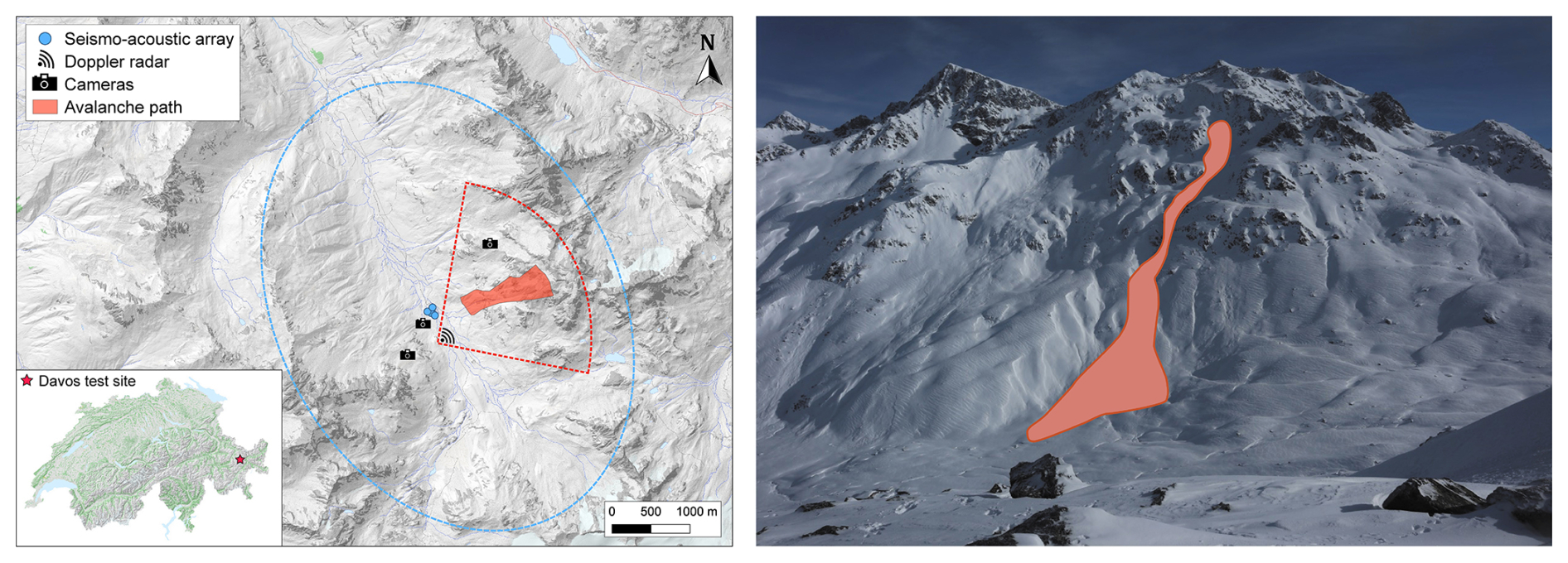
Figure 1Left: Map and location of the Dischma study site. The instrumentation consisted of a seismo-acoustic sensor array (blue dots), three cameras and a Doppler radar. The approximate area where avalanches could be detected is shown for the seismo-acoustic sensor array (blue ellipse) and the radar (red cone). Moreover, the red-shaded area highlights the same avalanche path as in the photo on the right. Right: Photo taken by an automatic camera at the study site, showing the georeferenced path of a dry-snow avalanche released on 2 February 2022 at 02:31 UTC.
Additionally, the site was equipped with a Doppler radar and three automatic cameras to obtain independent validation data, including accurate release times and information on the type and size of avalanches, provided favorable weather conditions. The radar emits electromagnetic waves that are reflected by the avalanche flow, providing the location and velocity of the moving avalanche (Meier et al., 2016). Figure 1 shows the location of the radar, which monitors several avalanche paths exposed to the west-southwest, covering an approximate area of 4 km2 (red delineated area). With this radar, avalanches could be detected up to a maximum distance of approximately 2 km. The cameras automatically photographed all surrounding slopes every 30 min (Fig. 1), which we manually inspected to identify days with avalanche activity and verify avalanche events of the detection systems.
In summary, the combination of detection systems installed at the study site allowed us to assess the limitations and advantages of each system individually, as well as their combined effectiveness for avalanche detection and characterisation. In this study, we focused exclusively on automatically detecting avalanches using seismic data. In contrast, we used the Doppler radar, cameras and acoustic systems to validate the detected avalanche events qualitatively.
From the continuous recordings of the seismic detection system (Sect. 2), we compiled an event catalogue for the winter seasons 2020–2021 and 2021–2022. Foremost, we collected avalanche signals detected by the radar and cameras. Additionally, we manually picked seismic events within periods of known avalanche activity (Sect. 3.1), ensuring to include avalanches that were not detectable by these other systems. Next, three experts labelled the events to compile a binary classification dataset (Sect. 3.2). Lastly, we prepared the signals of the event catalogue for model development (Sect. 3.3).
3.1 Event picking and signal processing
To define avalanche events, we selected signals based on the release times provided by the radar and automatic cameras. In addition, we picked potential avalanche events and other sources from the continuous seismic recordings that had been missed by the radar and cameras. Typically, the amplitude of seismic signals generated by avalanches gradually emerges (see Fig. 2) since the avalanche approaches the location of the seismic sensors at our study site (Fig. 1) and seismic energy radiates due to snow entertainment and erosion processes within the flowing avalanche (Pérez-Guillén et al., 2016). Therefore, automated picking methods often miss the starting phase of avalanches and sometimes entire events. To prevent this, we visually inspected the continuous seismic recordings and identified signals that exhibited a high signal-to-noise ratio, i.e. were not in the order of magnitude of the background noise. For efficiency, we limited our search to periods with known avalanche activity, such as avalanche cycles during snow storms, days when avalanches had already been detected by the radar and periods with observed avalanche deposits in the cameras.
For ease of picking the signals in those periods, we transformed the units of the raw recordings, i.e. counts, to meters per second (ground motion). Additionally, the signals were linearly detrended, tapered with a Hanning window and filtered with a 4th-order Butterworth band-pass filter between 1 and 10 Hz. We found this to be the most energetic frequency band of the avalanche signals recorded at our study site (Fig. 2), considering the typical relative distance between the avalanche and our receivers. To finally compile a clean event catalogue, we manually defined the onset and end times of the identified signals by visually inspecting the seismic signal, the envelope signal and the spectrogram. In total, we picked 912 events lasting between 5 and 515 s, which we labelled in the next step.
3.2 Event labelling
Having picked potential events, three experts assigned signals into two classes, avalanche and non-avalanche events:
- Avalanches:
-
Avalanche events were first identified using the radar and camera data (Fig. 1) by matching seismic signals to avalanches detected by the radar or on images. A second step to collect avalanches missed by these systems was to visually classify signals based on the characteristic seismic signature of avalanches (e.g. non-impulsive onsets, spindle-shaped signals and triangular-shaped spectrograms; left column in Fig. 2) as proposed by van Herwijnen and Schweizer (2011). Additionally, the output of wave parameters derived from sensor array processing of the seismic and infrasound data was considered, i.e. backazimuth angles and apparent velocity (Marchetti et al., 2015; Heck et al., 2018b).
- Noise (non-avalanche events):
-
Earthquakes were the most frequent source of environmental noise at our study site. They were identified by visual inspection of the signals (typical emergent onsets and usually identifiable arrival of the different phases; middle column in Fig. 2) and comparison of our seismo-acoustic recordings with two nearby seismic stations from the Swiss national network (Clinton et al., 2011). In addition, online earthquake catalogues were consulted to match our recordings with catalogued events (SED, 2023; EMS, 2023). The remaining portion of seismic events was generated by different sources, including aeroplanes (right column in Fig. 2), helicopters, explosions in nearby skiing resorts, weather events (e.g. wind), people or animals walking close to the sensors, and many more unknown event sources. We summarised this collection of unrelated events as a “noise” class. In particular, weak signals generated by non-verified small avalanches might also fall into this heterogeneous class. Moreover, this definition of the noise class barely included low signal-to-noise ratio (SNR) background noise.
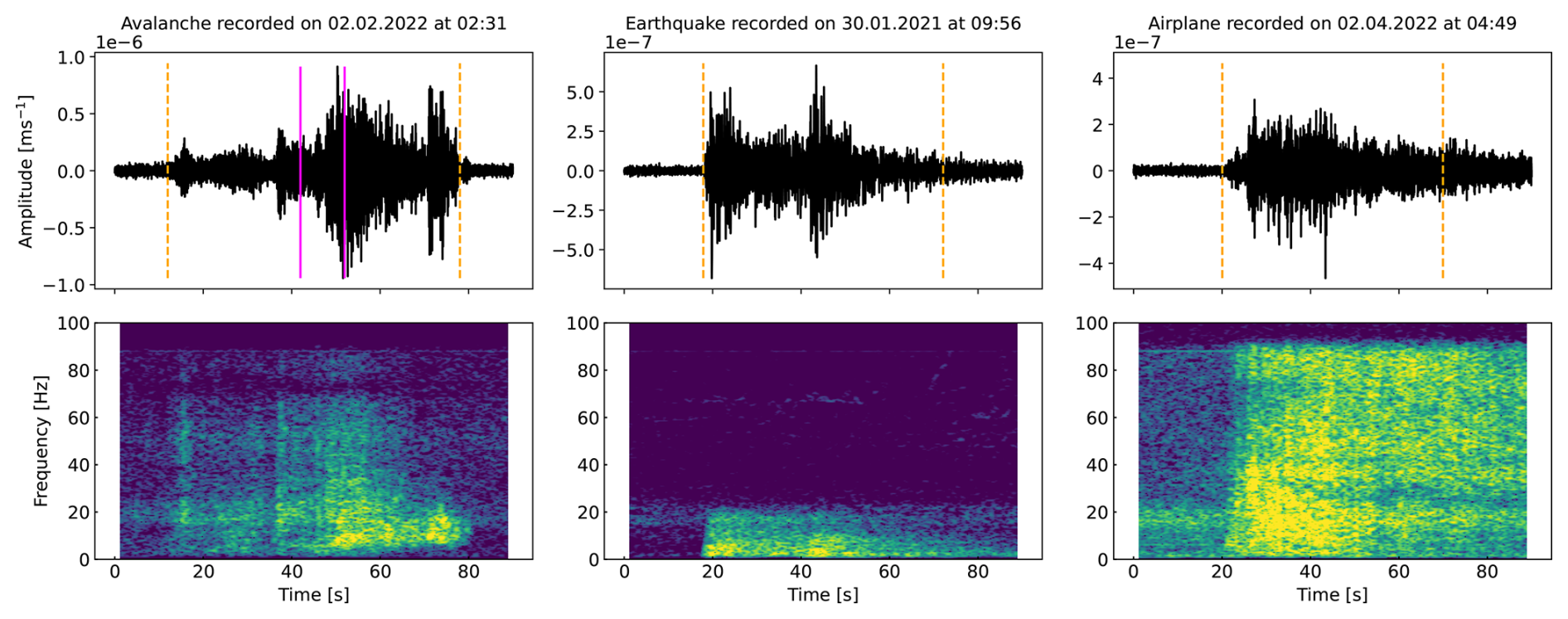
Figure 2Waveform and spectrogram of the avalanche in Fig. 1 (left), an earthquake (middle) and an aeroplane (right). The dashed orange vertical lines indicate the manually defined event onsets and ends. The pink vertical lines in the avalanche waveform indicate a 10 s seismic snippet extracted by the windowing algorithm. This specific signal window is highlighted later also in Figs. 4 and 10.
The three experts independently assigned subjective probabilities using either 0 (non-avalanche), 0.5 (potential avalanche) or 1 (certain avalanche). Note that the average rate of agreement in expert probabilities on the avalanche signals between the three experts was 58 %. This hints at the inevitable expert bias, the inherent subjectivity and the complexity of the task. Finally, a signal was labelled positive if the sum of the three expert probabilities was at least 2. In this manner, we compiled an event catalogue with 84 avalanches (31 verified with the radar or camera images) and 828 unrelated noise events from the 2020–2021 and 2021–2022 winter seasons. For completeness but not subject to the binary classification presented in this study, the same labelling process was used for earthquakes, with which we found 183 earthquakes in the noise class. The seismic sensors recorded maximum absolute amplitudes ranging from to m s−1 for avalanches, to m s−1 for earthquakes and to m s−1 for noise signals. Signal durations ranged from 13 to 113 s, 7 to 263 s and 5 to 515 s in each class, respectively. Notably, the noise class's amplitude range includes the avalanche class's amplitude range, highlighting its heterogeneity.
3.3 Signal windowing, normalisation and dataset splitting
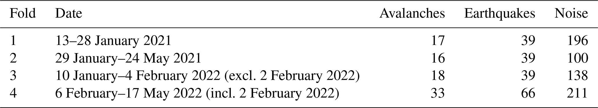
Aiming to enlarge the number of samples and develop a model pipeline for real-time detection, we further processed the signals of the event catalogue. Therefore, we used each seismic sensor's records independently, yielding five times more samples for model training. Second, we applied a 10 s moving window with 50 % overlap to all signals. This moving window algorithm resulted in again more data samples to train and ensured fixed-sized inputs for the models. Earlier studies (Lacroix et al., 2012; Hammer et al., 2017; Pérez-Guillén et al., 2019) have found the minimum duration of avalanches to be roughly ten seconds. Beyond, this strategy is also beneficial in a potential (near) real-time detection system, where 10 s windows are continuously parsed. Lastly, a crucial part when developing neural networks is input data normalisation (Sola and Sevilla, 1997). By applying the windowing algorithm, we obtained subsequences of time series. Since waveform characteristics of an upcoming event are not known in advance during inference, we normalised each window separately by its maximum absolute amplitude instead of using the maximum absolute amplitude of the entire event to avoid look-ahead normalisation (Rakthanmanon et al., 2012; Lima and Souza, 2023). With this, the labelled dataset comprised 3580 avalanche and 37 110 noise (non-avalanche) windows, which included 11 575 earthquake windows. Finally, we defined four independent data folds to develop the models and select the optimal architectures and their hyper-parameters (see Fig. 3). Three folds, comprising 70 % of the data samples, were used for model training and optimisation via 3-fold cross-validation. The test set (top bar in Fig. 3), containing 30 % of the data, was set aside to assess the model performance on an independent inference set. We separated the folds by specific dates to prevent any correlation and temporal data leakage between the folds. We chose the dates such that the class distributions across the folds were approximately balanced (Fig. 3). Additionally, we ensured that the independent test set included both dry and wet avalanches. This dataset was the foundation of model development and allowed for systematic comparison of the models in different settings.
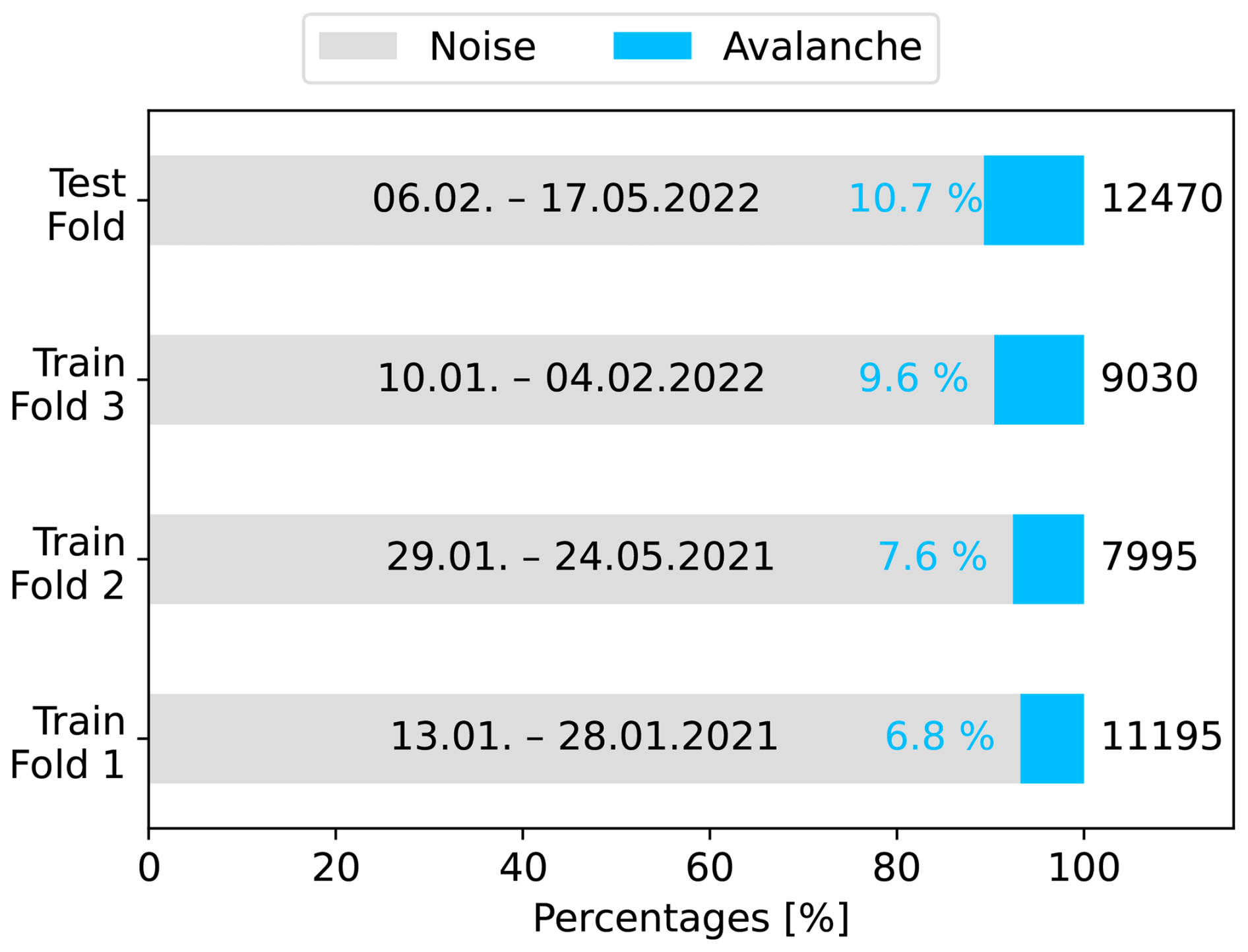
Figure 3Class distributions and date ranges in the train and test folds. The annotations at the end of the bars show the total number of 10 s seismic windows in each fold. The annotations in blue depict the percentage of avalanche windows.
For the later classification, we first extracted features from the 10 s signal windows (Fig. 4). Feature extraction generally describes the compression of a signal to a lower dimensional embedding to retrieve the signal's most distinctive information. The embedded information (the features) is usually used in an upstream classification or regression task. Following this framework, we explored three methods to extract information from seismic signals either as learned feature vectors or domain-specific engineered features, which are then classified as avalanche or noise. Concretely, we implemented a baseline based on a conventional expert-supervised feature engineering approach (Sect. 4.1) and developed two fully unsupervised autoencoders to extract features from temporal and spectral input data, respectively (Sect. 4.2). We then optimised three separate random forest models on top of the preceding feature extraction methods predicting avalanche and noise probabilities (Sect. 4.3).
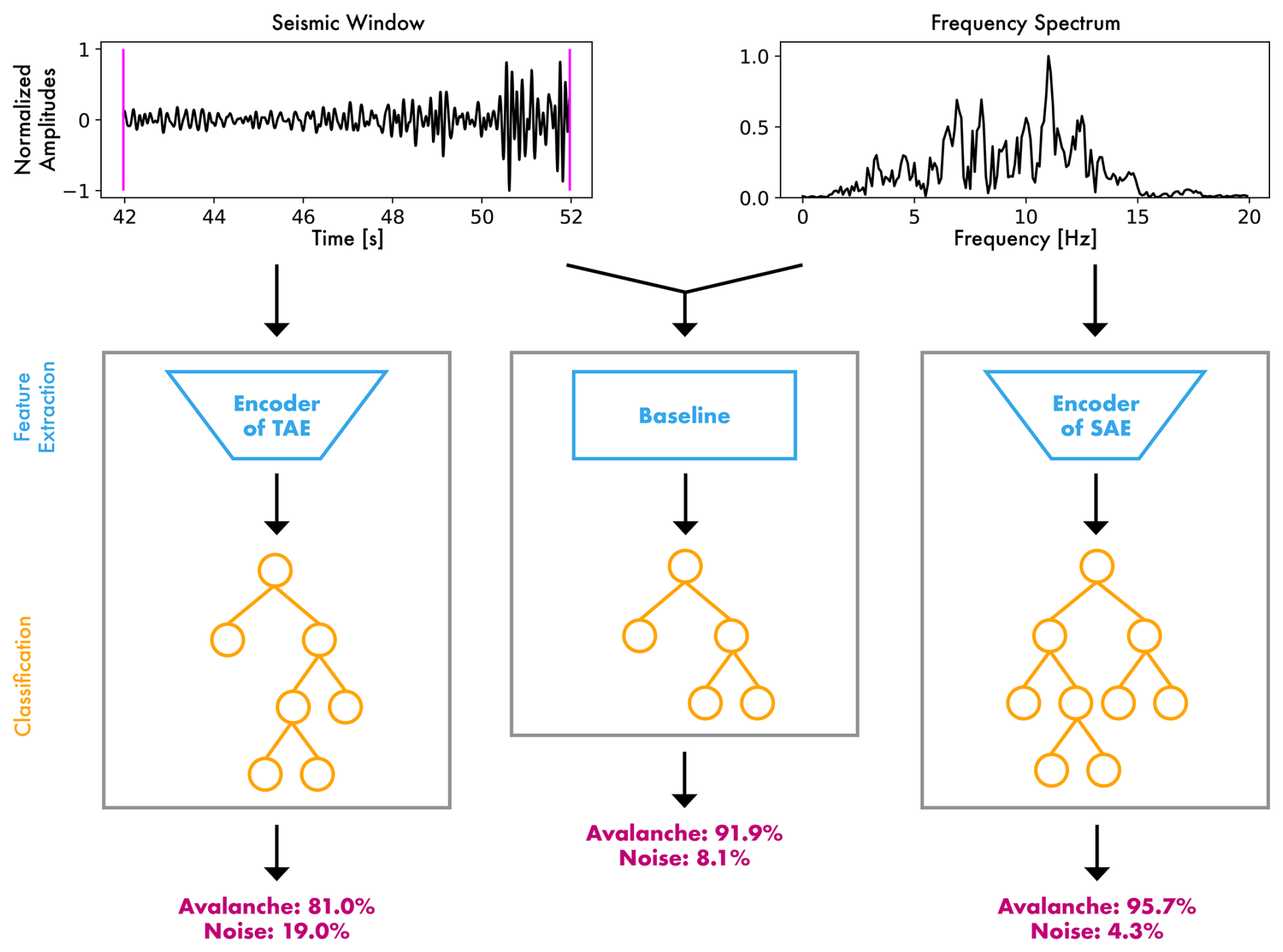
Figure 4Overview of the three methods to infer avalanche probabilities. The blue elements depict the feature extraction. During inference, the decoder of the autoencoders is discarded, and only the encoder is used to extract features. The orange parts show the classification using random forest models. The predictions are shown in pink for the given seismic window (the same as in the top left of Fig. 2). Left: The temporal autoencoder (TAE) feature classification; middle: The baseline classification using engineered seismic attributes; right: The spectral autoencoder (SAE) feature classification.
4.1 Baseline features
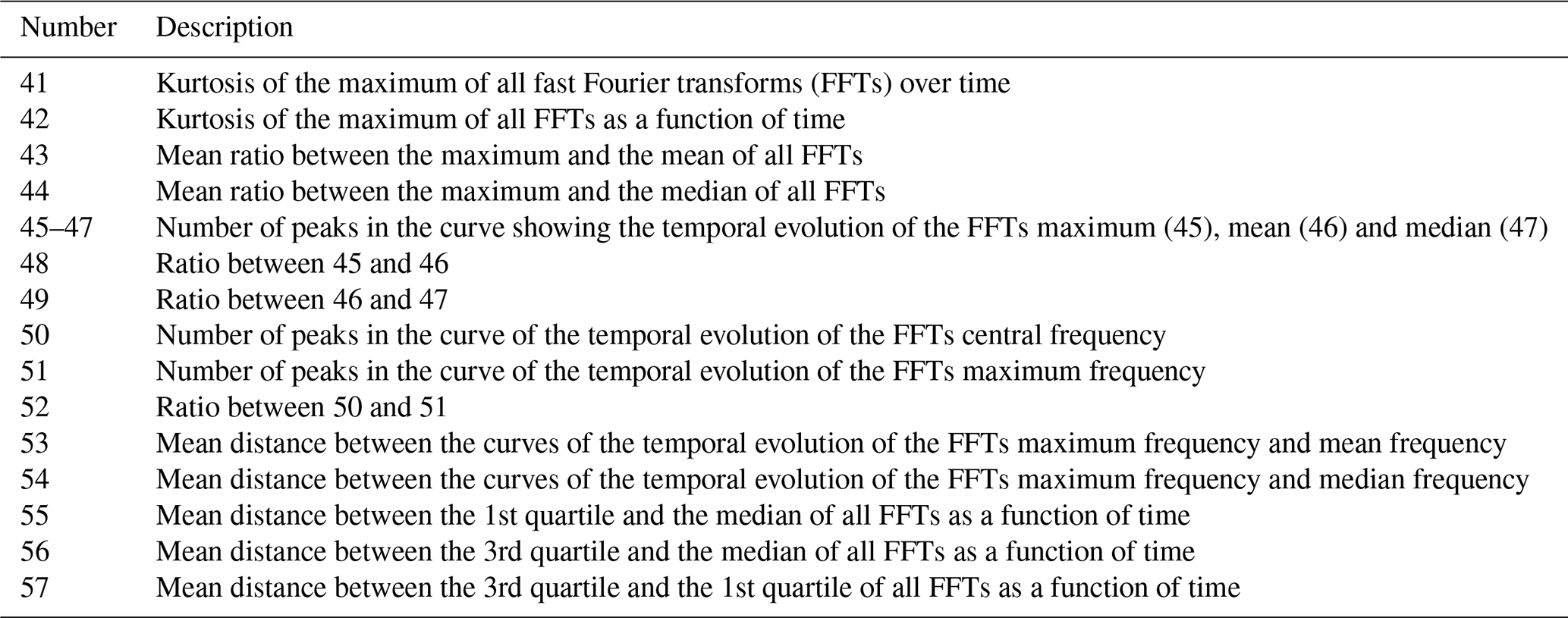
Since representation learning methods are a novel approach in seismic avalanche detection, we sought a baseline against which to benchmark them. Earlier studies on time series classification in general (Ismail Fawaz et al., 2019; Barandas et al., 2020) and on seismic detection of different types of mass movements (Rubin et al., 2012; Provost et al., 2017; Lin et al., 2020; Wenner et al., 2021; Chmiel et al., 2021) developed classification models using traditional feature engineering strategies. Therefore, in the baseline model, we followed a similar approach to Provost et al. (2017), which classified seismic events generated by landslides and extracted a set of 71 expert-engineered seismic attributes. Specifically, we used a subset of 22 waveform, 17 spectral and 18 spectrogram attributes (see Tables B1, B2 and B3 for more details). We extracted these from the frequency-filtered (1 to 10 Hz) 10 s seismic signals for all sensors separately. Additionally, we did not include network or polarity-related attributes since we aimed at developing models for a single-sensor setting and our study site was equipped with one-component sensors.
4.2 Autoencoder features
The autoencoder concept was first introduced by Rumelhart et al. (1986) and has since been adapted for various applications (Xugang et al., 2013; Mousavi et al., 2019; Gu et al., 2021). The architecture consists of an encoder and a decoder. The encoder compresses the input signal to a lower-dimensional embedding, i.e. the latent (feature) vectors. The decoder decompresses these feature vectors to the original input dimension. Overall, the autoencoder is trained by learning to reconstruct the input signals. Thus, by design, the encoder feature vectors are optimised to preserve the most distinctive information characterising a given input signal so that the decoder can reconstruct it. During inference, given that the autoencoder's purpose is to extract features for a classification process on top, the decoder can be discarded. The classifiers, which are trained separately, use solely the feature vectors.
4.2.1 Architecture
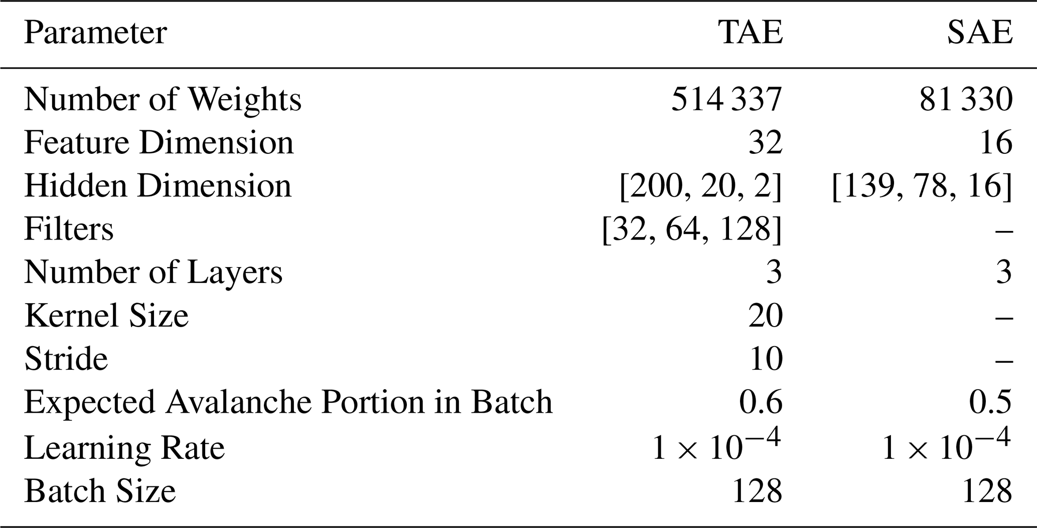
In the temporal autoencoder (TAE) we considered the seismic time series data, hence the name. It was developed for seismic waveform signals of 10 s, normalised by their maximum absolute amplitude. When dealing with time series data, common choices of computational units are one-dimensional convolutions (Kiranyaz et al., 2021) and recurrent units such as the long short-term memory cells (LSTM; Hochreiter and Schmidhuber, 1997). Thus, we implemented the encoder as a sequence of 3 convolutional layers and one LSTM cell layer learning temporal dynamics. The best model based on the optimisation procedure (Sect. 4.2.4 and Table E2) was composed of convolutions with kernel size 20 (or 0.1 s) and stride 10. This implementation of stride reduces the initial input length of 2000 samples (200 Hz × 10 s) to 200, 20, and 2 within each encoder layer. Similarly, the tuning procedure suggested 32 filters in the first convolutional layer, which we then doubled in each consecutive layer. In the last encoder layer, the LSTM cell summarises the output of the convolutions, i.e. two 128-dimensional vectors, to a feature vector of 32 dimensions (32 features). The decoder sequentially repeats this latent vector twice and applies three transposed convolutions with kernel size 20 and stride 10 to decompress the sequence back to its original length, i.e. 2000. Starting at 128 filters, we halved them in each decoder layer to reach 32 channels. To reduce this number to the number of input channels, i.e. 1, we applied a convolutional layer with kernel size 3 and stride 1 in the decoder output layer.
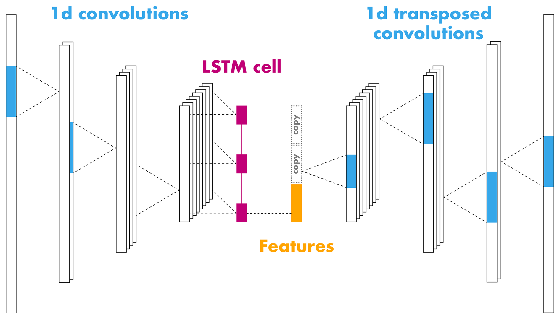
Figure 5Illustration of the temporal autoencoder architecture. The encoder comprises one-dimensional convolutional layers (kernels in blue) with leaky ReLU activation and batch normalisation followed by a long short-term memory cell (LSTM, pink). The decoder uses one-dimensional transposed convolutions to decompress the extracted encoder features (highlighted in orange) and reconstruct the input signal.
In addition, we used batch normalisation (BN) (Ioffe and Szegedy, 2015) in all encoder and decoder layers, except for the decoder output layer, to stabilise and accelerate training. As an activation function, we used the leaky rectified linear unit (leaky ReLU; Xu et al., 2015), which outperformed the tangent hyperbolic function (Tanh) during model optimisation. The only exception is again the output layer, where we replaced the leaky ReLU with the Tanh function to output values in the same range as the normalised input signals, which is . In summary, Fig. 5 gives a simplified overview of this architecture comprising 514 337 learnable parameters (226 848 in the encoder). This architecture is relatively small in the number of trainable parameters and, therefore, well adapted to the size of our dataset.
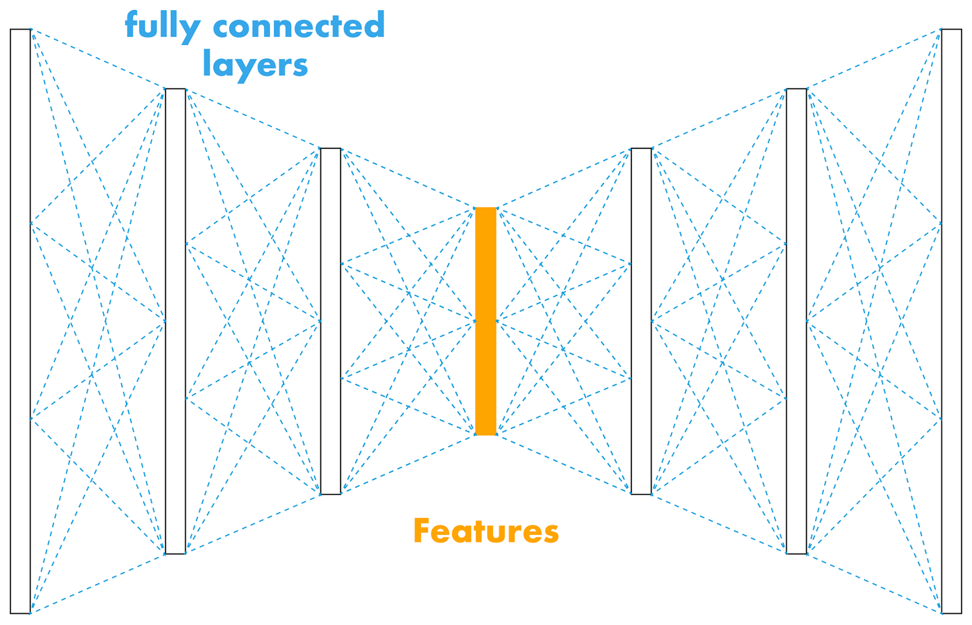
Figure 6Illustration of the spectral autoencoder architecture. The encoder and decoder are a sequence of compressing and decompressing fully connected linear layers (dashed blue lines). Each layer uses the hyperbolic tangent (Tanh) activation function and layer normalisation. The extracted features are shown in orange.
The second autoencoder implementation operates in the spectral domain, hence named spectral autoencoder (SAE). We used the fast Fourier transform (FFT) to convert the filtered 10 s seismic signals into the frequency domain. Thus, the input data to this model contained the amplitude spectrum normalised using the min-max normalisation. In contrast to the temporal autoencoder, we replaced the aforementioned computational units, i.e. convolutions and LSTM cells, with fully connected layers. Through hyper-parameter optimisation (Sect. 4.2.4 and Table E4), we designed the encoder and decoder to comprise three fully connected linear layers each. The hidden dimensions in the encoder evolved from 200 to 139, 78 and 16 (feature dimension). The decoder was a mirrored version of the encoder. Based on parameter tuning we used the Tanh function as non-linearity in all layers (Table E4). Moreover, we applied layer normalisation (LN) in each layer with the exception of the output layer. Figure 6 illustrates a simplified version of this architecture summing up to 81 330 learnable weights (40 589 in the encoder). As for the TAE, this architecture is even smaller and thus also well adapted to the size of the dataset.
4.2.2 Training regime
A training step in neural network optimisation starts with sampling a batch of predefined size from the dataset. For sampling, given that our dataset was severely imbalanced (Fig. 3), we used the so-called weighted random sampler, as implemented in PyTorch (Paszke et al., 2019). This sampling method oversamples the minority (avalanche) class and thus prevents the model from biasing towards the majority (noise) class. The sampling process relies on user-defined class weights, which allows the user to control the expected number of minority class (avalanche) samples within each batch. Therefore, we assigned the following relative weight to each sample of the avalanche class (wav), while we assigned the noise samples a weight of one (wno=1). Internally, the sampling method rescales and interprets these weights as probabilities.
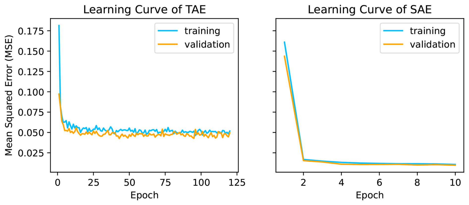
Pav is the user-defined expected portion of avalanches per batch, e.g. 0.5 for evenly balanced batches, while Nav and Nno are the number of avalanche and noise samples respectively. The batch is then passed through the entire network (forward pass) to produce the output (prediction). The output is compared to the target and the mean squared error (MSE) reconstruction loss is computed (see Eq. C1). The network weights are then optimised by computing the gradients of the loss function and propagating them back through the network (back-propagation) using the Adam optimizer (Kingma and Ba, 2014) with a specified learning rate. After, the next batch is passed to the network repeatedly until all batches in the dataset have been seen once, which defines an epoch. The entire process is then again repeated for a certain number of epochs. Figure E1 in the appendix illustrates the training and validation progress per training epoch for the temporal (TAE) and spectral autoencoder (SAE).
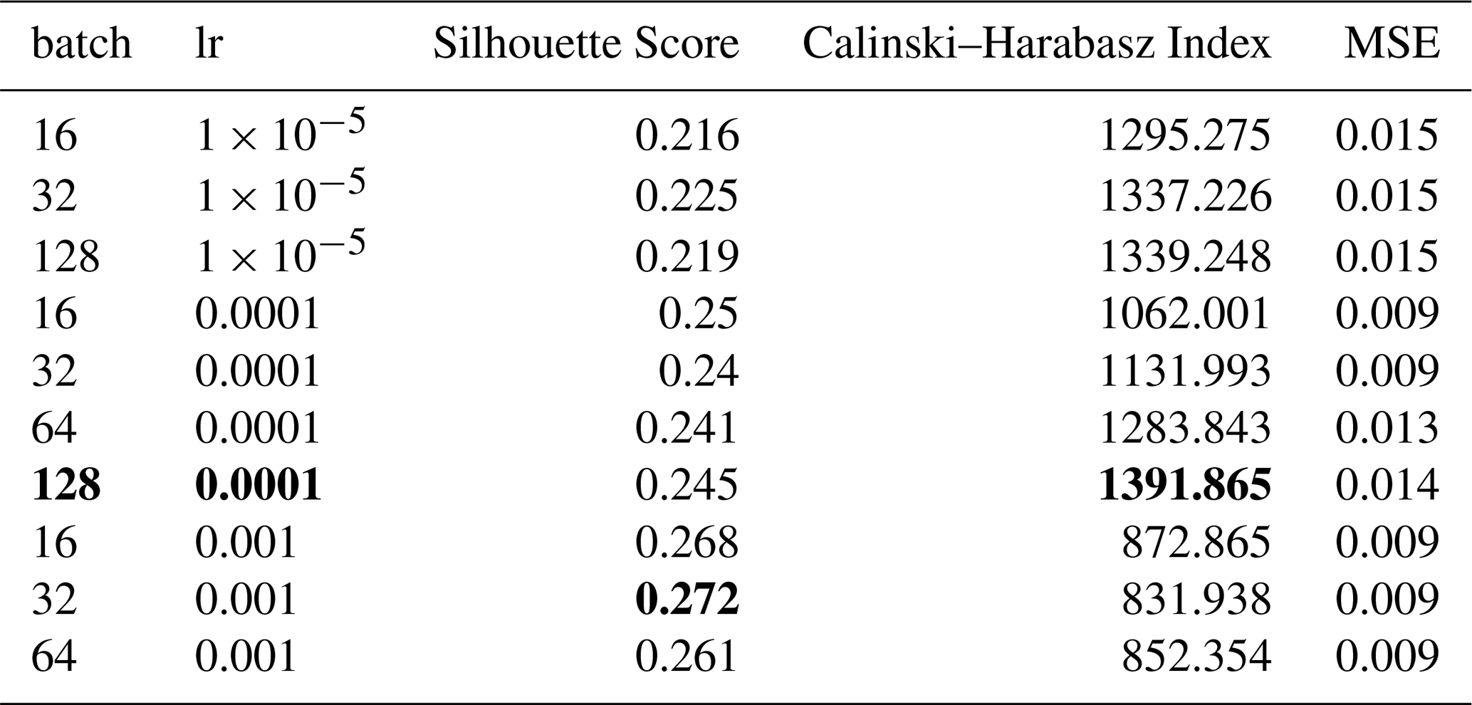
Following our hyper-parameter tuning strategy, we found the temporal autoencoder training optimal with an expected portion of avalanches per batch of Pav=0.6, a learning rate of and a batch size of 128 (Table E3). The model was trained for 120 epochs, i.e. iterations through the entire dataset, with early stopping when the class-separation metrics (Sect. 4.2.3) started decreasing. Additionally, we applied data augmentation by randomly shifting the 10 s signals by 0 to 1 s to either the right or left to reduce overfitting in the avalanche class and for better generalisation (Zhu et al., 2020). Similarly, in the spectral autoencoder training, we used an expected portion of Pav=0.5 avalanches per batch, a learning rate of and a batch size of 128 (Table E5). Moreover, we found five training epochs to be optimal.
4.2.3 Validation
In addition to the training regime (Sect. 4.2.2), we defined a validation routine for comparing different autoencoder architectures and settings in the model optimisation (Sect. 4.2.4). By definition, the autoencoder performance can be measured with its reconstruction loss. However, given a decent reconstruction, we aimed to find the best input features for the later classification. Hence, we evaluated the autoencoders based on the avalanche and noise class separation within the latent (feature) space. We calculated the silhouette score (Rousseeuw, 1987) and the Calinski-Harabasz index (Caliński and Harabasz, 1974) based on the feature embedding location and their given expert labels (see Appendix C3). We selected the best autoencoder by searching for the highest-ranking combination of silhouette score, Calinski-Harabasz index and the mean squared error loss.
4.2.4 Model selection
Developing neural networks involves tuning network hyper-parameters, such as the number of layers, kernel sizes of convolutions or hidden dimensions. Therefore, we used the three training folds in Fig. 3 to run 3-fold cross-validation. Using three folds reduces the impact of data variability and yields more reliable performance estimates. Next, we defined a grid of hyper-parameter combinations (Table D1) and iteratively trained the resulting model configurations on two and evaluated them on the left-out fold. We selected the model showing the best average performance over all three folds according to the predefined validation metrics (Sect. 4.2.3). Besides the internal network parameters, we applied the same procedure to tune the parameters of the training regime (Sect. 4.2.2). Concretely, we searched for the optimal number of expected avalanche samples in each batch (Pav in Eq. 1), the learning rate and the batch size. Details of this process can be found in the Appendix E.
4.3 Feature classification
Foremost, this work aims to detect avalanches in seismic recordings. Therefore, the previous extraction of distinctive features was only an intermediate step. To classify these features, we developed three random forest classifiers – one per feature extraction method. We tuned them for the baseline, the temporal and the spectral autoencoder features separately to infer class probabilities (see Fig. 4).
4.3.1 Random forest model
The random forest model is a widely used algorithm for classification in general and for seismic event detection in particular (Provost et al., 2017; Li et al., 2018; Chmiel et al., 2021), as it is favourable when dealing with high-dimensional features and heterogeneous (e.g. engineered features) input data. The algorithm was introduced by Breiman (2001) and belongs to the class of ensemble methods. During training, several decision trees (estimators) are grown. Each tree is grown on a different bootstrap sample of the original dataset, i.e. a random draw with replacement. Instead of using the entire set of features in the original dataset, a random subset is assigned to each node in the tree individually. The split (branch) is based on a single feature from this random subset, which is optimal under a specified splitting criterion, such as the Gini information criterion (Breiman, 2017) when dealing with categorical (classification) splitting problems.
4.3.2 Cross-validation
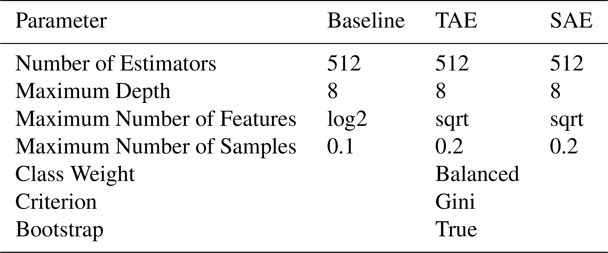
In search of the best hyper-parameters of this tree-growing algorithm, e.g. the maximal number of estimators (trees), we used a randomised grid search with 3-fold cross-validation. This method evaluates hyper-parameter combinations by iteratively fitting the random forest model to two of the three training folds (Fig. 3) and validating it on the left-out fold. As a scoring function, we chose the avalanche class F1-score to weight the avalanche precision and recall uniformly and averaged this score across the three folds. This optimisation process was applied with the three feature sets individually, i.e. the baseline and autoencoder features, to find the random forests presented in Table D1.
4.3.3 Inference and post-processing
During inference, a (test) feature vector is first passed separately to each decision tree in the random forest. Each tree applies its learned sequence of decision rules and classifies the feature vector as either avalanche or noise. Then, each tree's classification is aggregated by computing the mean. For instance, assuming 90 out of 100 trees classified a given feature vector as an avalanche, this sample was assigned an avalanche probability of 0.9, estimated as the fraction of votes within the forest. This process, known as ensembling, is why the random forest algorithm is considered an ensemble method. The only parameter to define was a probability threshold above which, we classified the sample as an avalanche. We used the default threshold of 0.5, which means a sample was classified as an avalanche if at least half of the trees agreed on this classification. Hence, for a single 10 s seismic signal, the random forest models provided both a binary classification (avalanche or noise) and the probability for each class.
Then, in the first post-processing step, we leveraged the array of five seismic sensors deployed at our study site and aggregated the per-sensor model output probabilities, computing a multi-sensor avalanche probability for each 10 s window. The array-based avalanche probability was calculated as the mean of the individual probabilities from each sensor. In the second post-processing step, we revisited the offline avalanche activity monitoring or dataset labelling objective by evaluating the classifiers on entire events rather than single 10 s windows. Therefore, we considered an event an avalanche if at least two (overlapping) consecutive windows (i.e. 2×10 s − 0.5×10 s =15 s of an event) had been positively predicted. Given that the shortest avalanche in the dataset was 13 s, we considered this boundary feasible. The reason for not aggregating the probabilities over the event length or similar was that in a continuous application, such as avalanche activity monitoring or labelling of an unannotated dataset, the event length is unknown.
With this post-processing, we could evaluate the performance of the random forest classifiers based on single-sensor, sensor array-based and event-based detections.
After model development completion, we evaluated the baseline, the temporal autoencoder (TAE) and the spectral autoencoder (SAE) on the unseen test fold (top bar in Fig. 3). To assess the models' stability, we trained and tested them using 20 different random seeds, i.e. powers of two starting with 20. Therefore, we calculated the mean and standard deviation of all metrics, while for specific result analysis, e.g. Fig. 10, we used the random seed for which a the model showed the highest avalanche F1-score (25 for the baseline, 216 for both autoencoders).
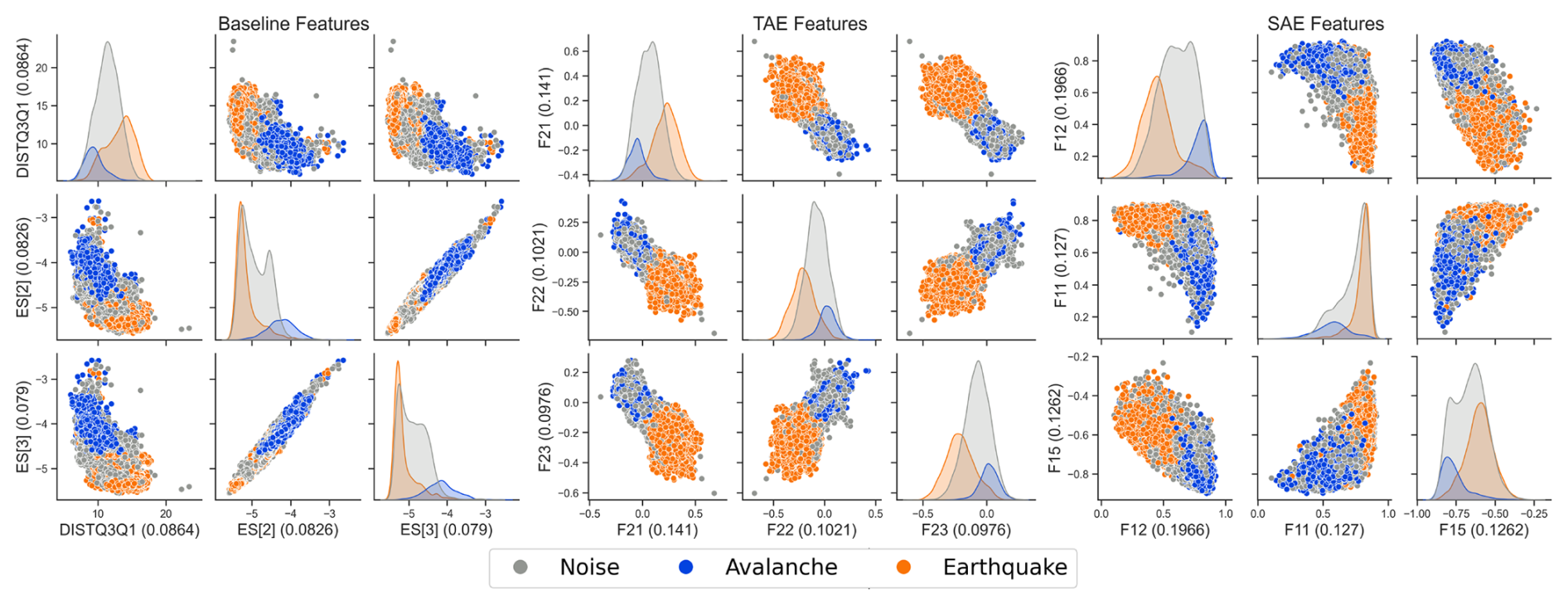
Figure 7Test set latent space visualisation of the most important features according to the impurity-based feature importance (value in parenthesis) of the random forest models for the baseline (left), the TAE features (middle) and the SAE features (right). In the left plot, DISTQ3Q1 is the mean distance between the 3rd and the 1st quartile of all FFTs as a function of time, ES[2] and ES[3] is the energy in the frequency band [5, 7] Hz and [6, 9] Hz respectively (features 57, 35 and 36 in Tables B3 and B2). The axis labels starting with the letter “F” in the middle and right plot represent a specific autoencoder feature carrying no explicit physical meaning.
5.1 Single-sensor predictions
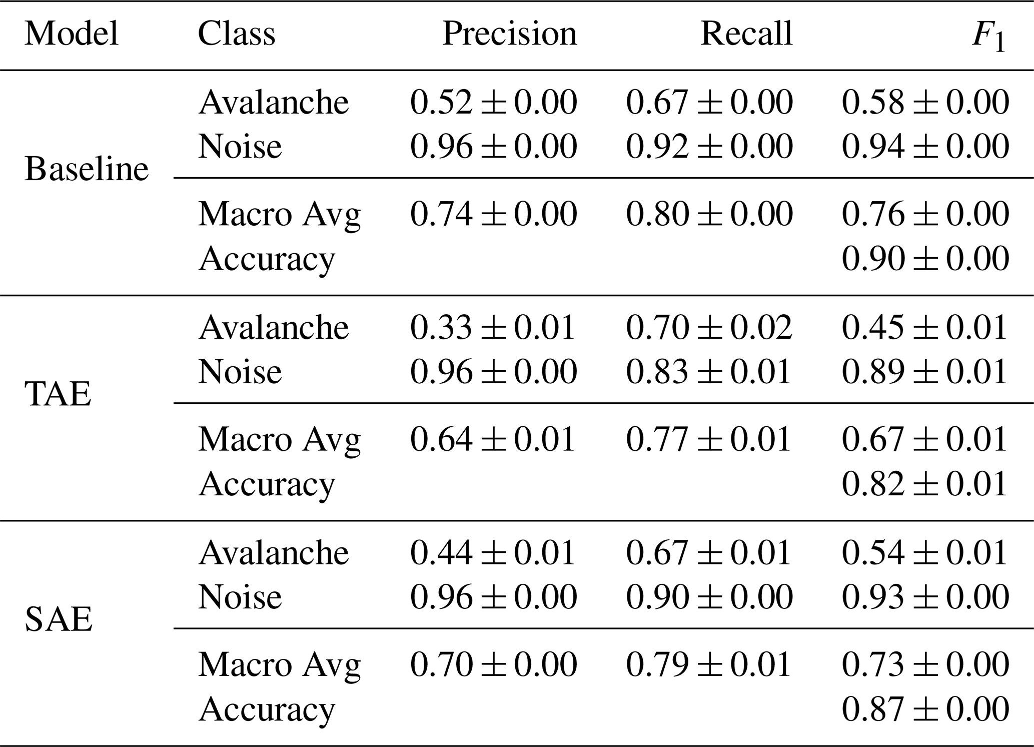
As a first step, we evaluated the detection performance of each model's single-sensor predictions on the 10 s seismic signals. The true positive rates (or avalanche recall) were similar across the models (Fig. 8), i.e. between 67.3 % (±1.4 %) and 69.8 % (±1.8 %), indicating that approximately 30 % of all avalanche windows were missed. Nevertheless, the avalanche recall was highest for the TAE features classification. Regarding the true negative rates (or specificities), i.e. the probability that an actual noise event will be predicted as noise, we noted that the TAE features classification showed the lowest rate of 83.0 % (±1.0 %) and, therefore also showed the lowest avalanche precision of 0.33 (±0.01), compared to 0.52 (±0.00) for the baseline and 0.44 (±0.01) for the SAE (Table 1). Thus, we expect this model to produce comparably more false alarms (false positives) at a rate of 17.0 % (±1.0 %). Overall, the macro-average F1-score reached values of 0.76 (±0.00), 0.67 (±0.01) and 0.73 (±0.00) for the baseline, the TAE features and the SAE feature classification respectively (Table 1).
Additionally, since the feature extraction and its information content are core concepts of this study, we visualised part of the latent spaces in Fig. 7. As earthquakes account for a significant proportion of the noise class (31 %) and labels were available anyway, we showed them separately. This visualisation provided some insights into the organisation of the latent spaces. For instance, all models spatially separated avalanche and earthquake samples.
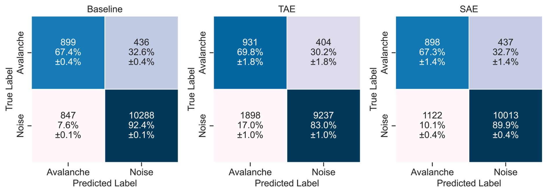
Figure 8Confusion matrices of the binary classification results for the three feature sets on the held-out test fold data, including all five sensors. The rows indicate the true (expert) labels, while the columns provide the predicted labels of the random forest classifiers. The colours code the percentage values.
Table 1Classification metrics on the (unseen) test fold data comprising 1335 avalanche and 11 135 noise samples for the three feature sets. Due to the strong class imbalance, the weighted averages of the metrics are not shown.
5.2 Sensor array-based predictions
In addition to the predictions on the individual 10 s windows, we aggregated the single-sensor predictions over the five sensors in the seismic array by averaging the single-sensor output probabilities, resulting in improved model performance (Fig. 9). The macro-average F1-scores increased by 2.6 % (baseline), 4.5 % (TAE) and 5.5 % (SAE). This improvement particularly originated from lower false positive rates, while the rate of missed avalanche windows remained at about 30 % in all models. After aggregation, the baseline and the SAE feature classification yielded similar performance in the classification metrics (see Table 2). The TAE feature classification, however, still showed approximately double the number of false alarms, i.e. 308 (14.0 % ±0.8 %), compared to the other models despite this improvement. The sensor array-based aggregation further enabled us to investigate how predictions evolve over an entire seismic signal (Fig. 10). For the avalanche shown in Figs. 1 and 2 (left), the models were uncertain in the starting phase, when the avalanche amplitudes slowly emerged from the background noise signal. However, as the signal became more energetic, the avalanche probability increased for all models. Overall, this post-processing strategy reduced the number of false alarms and slightly improved the avalanche recall.
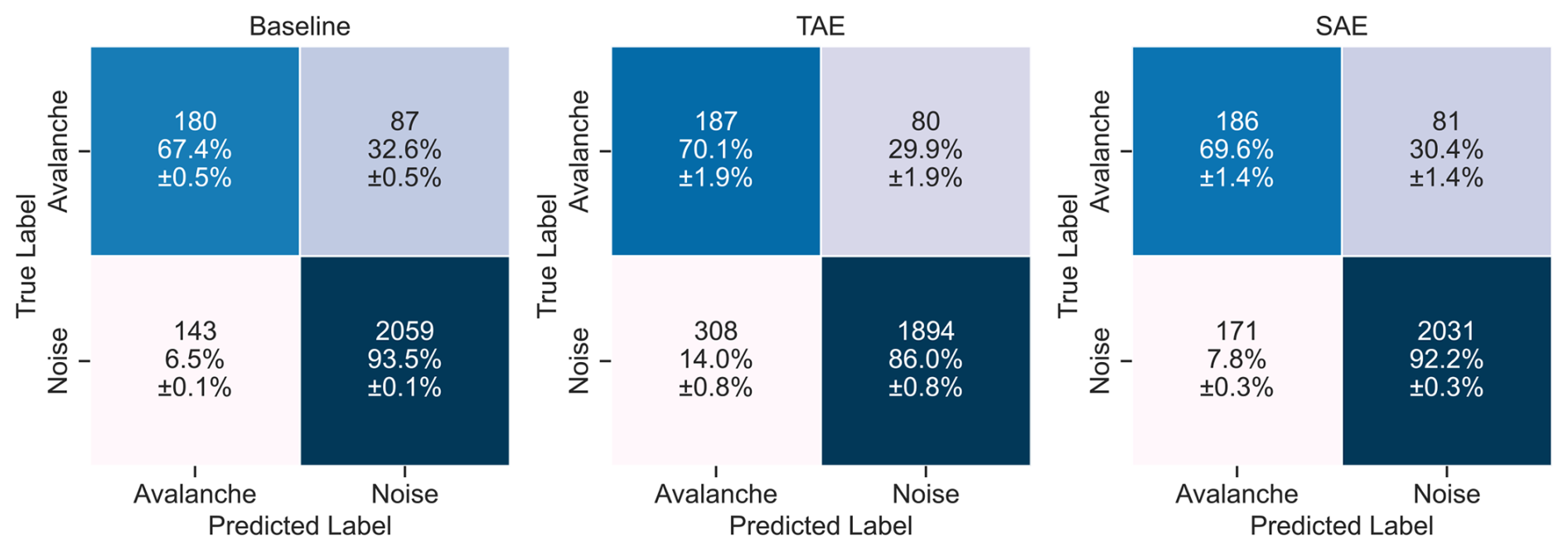
Figure 9Results on the held-out test fold data after applying a probabilistic aggregation of the single-sensor 10 s predictions over the five sensors of the sensor array. The rows indicate the true (expert) labels, while the columns provide the predicted labels of the random forest classifiers. The colours code the percentage values.
Table 2Classification metrics on the (unseen) test fold data comprising 267 avalanche and 2202 noise samples after probabilistic aggregation over the five sensors. Due to the strong class imbalance and bias towards the noise class, the weighted averages of the metrics are not shown.
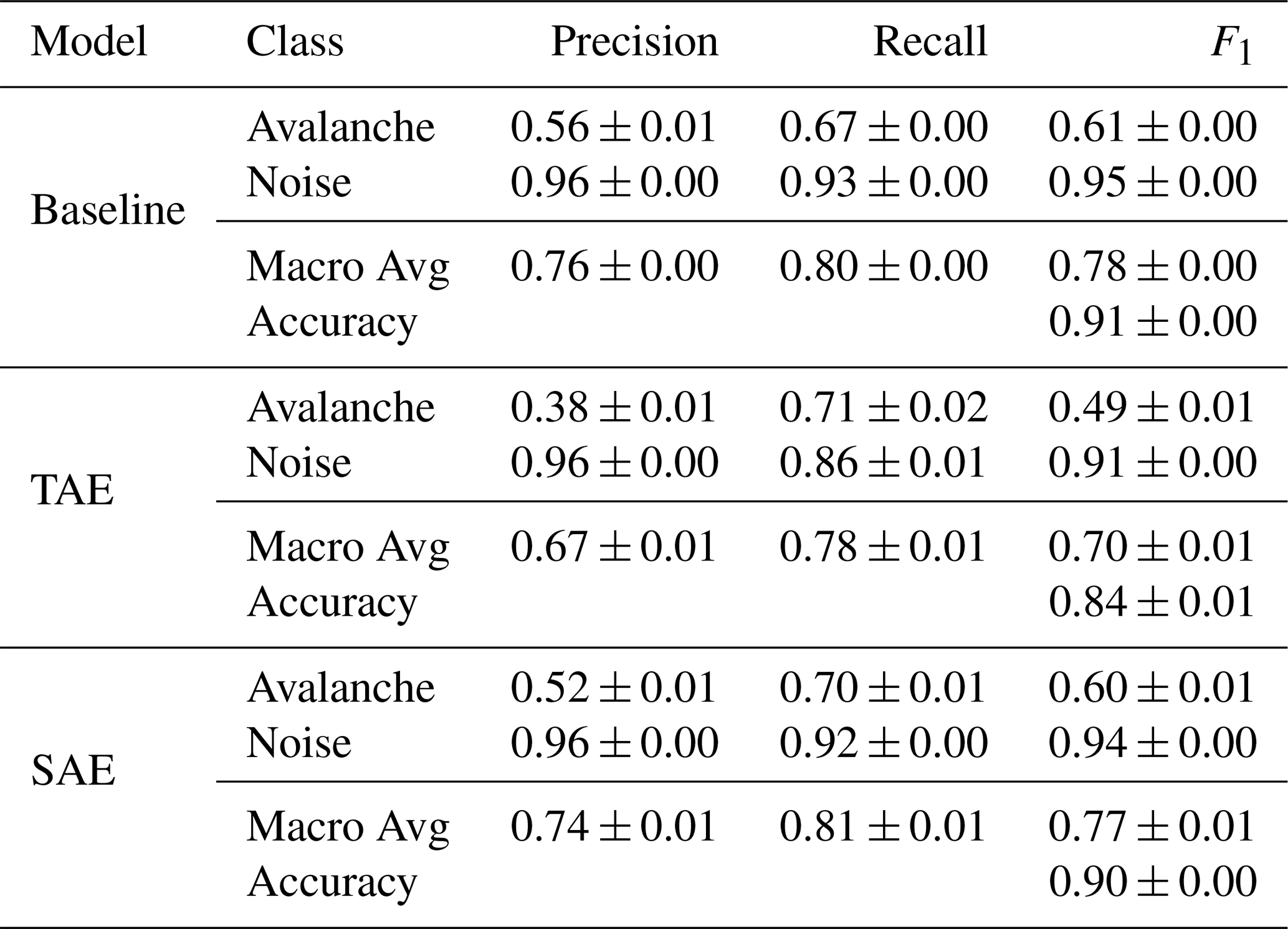
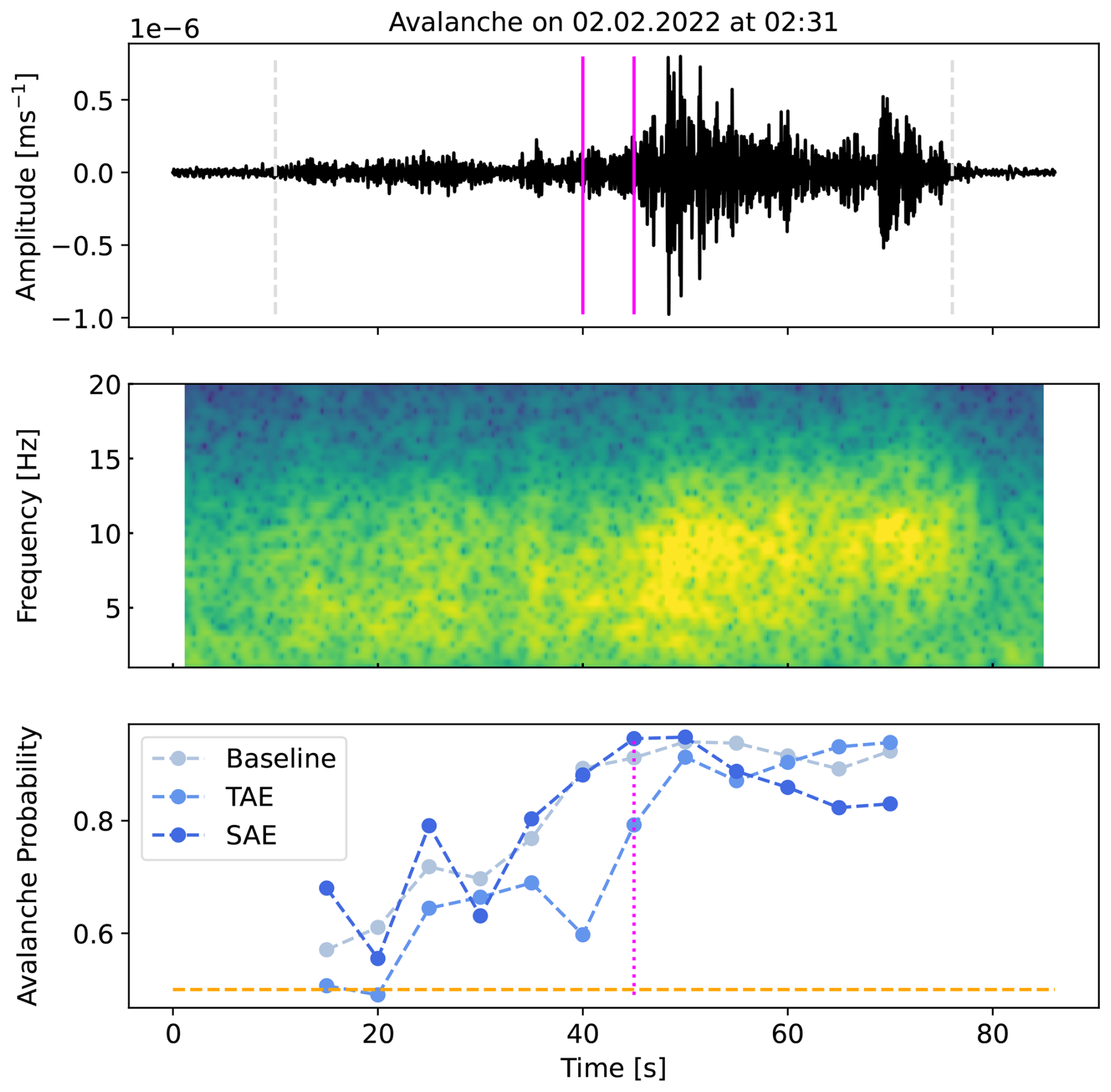
Figure 10Waveform and spectrogram generated by the avalanche in Fig. 1 and the array-based output probabilities for each model over the entire avalanche signal (bottom). The signals have been filtered from 1 to 10 Hz corresponding to the input frequency band of the models. In pink, the same 10 s seismic window as in Fig. 2 (left) and Fig. 4 is shown and the according probabilities are highlighted (lower plot). The probabilities are computed as the average of the single-sensor probabilities predicted every 5 s (10 s windows with 50 % of overlap). The manually defined event onset and end are highlighted in dashed grey lines (upper plot), and the classification threshold 0.5 is in orange (lower plot).
5.3 Event-based predictions
Besides the single-sensor and array-based predictions (Sect. 5.1 and 5.2), we investigated the predictions on an event basis to close the gap to avalanche activity assessment and provide a broader outlook. For this, we assigned an event to the avalanche class if two consecutive 10 s windows (50 % overlap) of the sensor array-based predictions were detected as avalanche signals. This post-processing led to the results in Fig. E2 and Table E6 in the Appendix E2. Although the overall performance of the three models decreased by about 5 % (see Table E6), the true positive rates (avalanche recall) increased significantly to 81.4 % (±1.1 %) (baseline), 84.8 % (±2.6 %) (TAE) and 89.3 % (±4.3 %) (SAE). Hence, by applying this step, the spectral autoencoder could successfully detect 89.3 % (±4.3 %) of all avalanches in the test fold.
So far, we compared the performance of the baseline, an expert-engineered seismic attribute classification, and the autoencoder feature classifications based on a dataset containing 10 s seismic signals in a single-sensor, sensor array-based and event-based setting. In the single-sensor setting, the models missed approximately 30 % of all avalanche windows and produced false alerts at rates between 7.6 % (±0.1 %) and 17.0 % (±1.0 %). With the sensor array-based aggregation, we observed a reduction in false alarms and a slight improvement in avalanche recall. In the event-based setting, we compromised an improvement in avalanche recall with an increase in false alarms. Moreover, we noticed that the automatically learned features, specifically the ones from the spectral autoencoder, performed comparably to the baseline. Hence, the results showed that spectral input information seemed favourable. In the following, we contextualise the results by investigating the detection errors and their possible origins. Therefore, we summarise the model development (Sect. 6.1) and focus on the false predictions of the models to find potential limitations (Sect. 6.2 and 6.3). Finally, we argue about the applicability of these models (Sect. 6.4) and compare the results to previous work (Sect. 6.5).
6.1 Model performance and limitations
The quality and size of the dataset strongly influence deep learning models. The relatively small size constrained us to design autoencoder architectures with few trainable parameters. In addition, we used each sensor independently to compensate for dataset size, as each sensor can be considered a different view of the same event. However, this came at the cost of introducing correlation among dataset samples as the sensors were installed nearby (Fig. 1) and thus recorded very similar signals, yet not necessarily adding much new and enriching information to the dataset. Given that the dataset will increase in the upcoming winters, we will consider incorporating the five sensors as distinct channels in a convolutional and/or recurrent model in future studies. With this, the sensor array-based aggregation and fusion would be implicitly implemented into the model.
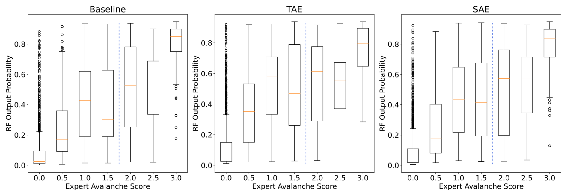
Figure 11Sensor array-based output probabilities of the random forest models for their respective input features plotted against expert avalanche scores. The blue dashed line indicates the threshold applied to the expert scores to assign avalanche class labels.
Another aspect to consider was our approach to normalise each 10 s seismic window independently. Normalising input data has proven crucial when training neural networks (Sola and Sevilla, 1997). The temporal autoencoder, in particular, therefore lost information on absolute and relative amplitudes. Yet, both autoencoders could still capture signal characteristics and remarkably showed similar patterns when looking at continuous predictions and comparing with the baseline (see Fig. 10). Alternatively, a normalisation over the entire signal before applying the windowing algorithm could be envisioned to preserve information on relative amplitudes. However, this normalisation is not applicable during an online inference, as it would require looking ahead at the amplitudes of the incoming waveforms. Therefore, it is not practical for (near) real-time signal classification. Alternatively, normalising by a characteristic value of the training dataset is unfavourable considering the heterogeneity of the data and a future implementation at another study site with potentially completely different characteristics. Also, note that normalising by class characteristics of the training data would violate the unsupervised learning regime.
Further, the separation of the feature extraction and classification process was driven by the dataset at hand and the success of representation learning in various applications (Bengio et al., 2013; Längkvist et al., 2014). Considering the data, the unsupervised feature extraction was not constrained by class labels (only the model selection and hyper-parameter tuning of the classifiers were), an advantage when dealing with non-ground-truth labels (two-thirds of the avalanches were neither verified by the radar nor the cameras). The applied expert labelling to the non-verified events was subject to an unknown degree of subjectivity and belief. We found the average agreement rate of the avalanche expert probabilities to be 58 %, meaning two experts agreed on 58 % of the avalanches. In addition, having decided upon a hard threshold to convert expert scores to class labels further blurred the boundaries between the avalanche and noise class, potentially including minor avalanches in the noise class (false negatives). Apart from the event label uncertainty, we considered the subjectivity of manually defining event onset and end and the uncertainty of adopting the event labels to the 10 s snippets after applying the windowing algorithm. Due to the attenuation of avalanche signals with the distance to the sensors and the low initial energy of avalanches, some 10 s windows containing primarily background noise within an avalanche event were inevitably mislabelled (false positives). This particularly applies to a signal's starting and ending sections (see the upper plot in Fig. 10).
In summary, all of the above led to the conclusion to explicitly separate the feature extraction from the classification and implement an unsupervised learning approach, which is more robust to uncertainty and noise in the labels and could leverage more unlabelled data. In contrast, a fully supervised neural network might suffer from the relatively low number of labels and bias, tending to overfit these expert labels rather than learn avalanche characteristic patterns in seismic signals. Moreover, the developed autoencoder approaches offered better comparability with the baseline model, i.e. feature engineering.
This separation then allowed us to analyse a lower-dimensional embedding of the dataset by inspecting the feature space distributions (Fig. 7). As labels for earthquakes were available, we visualised them separately. Moreover, earthquake and avalanche signals can be similar in the time domain (Heck et al., 2018b), thus we wanted to investigate them in the feature domain. Overall, the three event types, i.e. avalanches, earthquakes and rest, varied in the encoding locations, yet also showed considerable overlap. Interestingly though, the avalanche and earthquake signals were well separated (blue and orange in Fig. 7). The rest (grey) resembled a connecting cloud between avalanche and earthquake signals. The reason for this might be two-fold; first, the heterogeneity of these noise events by potentially comprising minor avalanches and low magnitude earthquakes (false negatives), and second, the strong attenuation in some sections of avalanche signals resulting in low amplitude avalanche windows. The former noise class heterogeneity originated from comprising different sources in comparable amplitude ranges, e.g., earthquakes, aeroplanes or strong wind. However, these various sources are definitive to be expected and need to be considered in a real-time detection system.
Despite actually having earthquake labels, we opted for a binary classification. In an early stage, we trained models with three classes (earthquake separately), without seeing an increase in overall model performance. This came as no surprise when looking at the clear separation of the earthquake from the avalanche samples in latent space. Moreover, training a model to also classify earthquakes was out of scope as these can be detected with other methods. Thus, we did not consider earthquakes a separate class in the classification. However, considering the avalanche class, investigations could also be conducted by differentiating between type and size in future implementations. Since the primary goal of this study was to develop and compare models to detect avalanches regardless of their type or size, we trained the models considering all the recorded avalanches. Therefore, we ensured that various avalanche types were included in the train and test set by separating them based on appropriate dates (Sect. 3.3). According to radar and image data, most avalanches detected at our study site ranged between sizes 2 and 3, based on the European avalanche size classification (EAWS, 2021). Given that seismic patterns of avalanches are influenced by the avalanche type (Pérez-Guillén et al., 2016), an alternative approach could be to develop two independent models to detect dry-snow and wet-snow avalanches separately. However, the current dataset was too small to further categorise the avalanche events by size and type, and accurate ground-truth data was often also missing. Instead, we focused on the given and analysed the misclassification of the current models.
Finally, to obtain an intuition and analyse how the supervised random forest classifiers related to the expert scores, we plotted the expert scores of potential avalanche signals against the model's output probabilities (Fig. 11). Overall, the output probabilities positively increased with the expert scores. As expected, we also noted the highest uncertainty at the selected threshold (dotted blue line in Fig. 11). When comparing the feature sets, the classification with the baseline features yielded more apparent steps over expert scores and more distinctive probabilities for the highest and lowest expert scores. A measure to mitigate having to deal with such noisy labels in future works might be to include verified avalanches solely and discard the non-verified ones for training the models. However, the unsupervised autoencoders are entirely independent of any labels or class information. Thus, by considering only verified avalanches, we would not reduce class ambiguity from the autoencoder’s perspective, but the dataset size and with it, valuable information might be lost.
6.2 Missed avalanche windows
As avalanches were this work's main objective, we first analysed the missed avalanche windows, i.e. the false negatives (FNs). Looking again at Fig. 11, we accredited the relatively high number of outliers (FNs) in the expert score of 3, i.e. verified avalanches, to the nature of mass movement signals. Concretely, avalanche signals slowly emerge from the background noise due to source-receiver distance and the low generation of energy in the initial and very end stages of avalanche motion, resulting in the typical spindle-shape signal with a relatively low signal-to-noise ratio at the beginning and end of the signal (Suriñach et al., 2001; van Herwijnen and Schweizer, 2011; Pérez-Guillén et al., 2016). We suspect the models had difficulties correctly classifying these parts of an avalanche signal producing FN predictions. Further, the manual definition of event onset and end was rather generous in including the entire avalanche signal with parts characterised by very low amplitudes and potentially also some background noise was included. For instance, Fig. 12 shows a comparison of the time series of sensor array-based predictions for each model with the misclassified onset of an avalanche event in the left plot, while in the right, the end portion was characterised by a very low signal-to-noise ratio and hence misclassified. In Fig. 12 (left), the first few time windows from 10 s to approx. 35 s are arguably rather noisy, as suggested by the model probabilities. Though as the signal strength increases, model probabilities also increase. Concretely, if we considered the first five predictions or time windows, this sample accounts for 5 (non) FNs in the results in Fig. 9 and 25 (5 sensors × 5 windows) in Fig. 8 per model. The sensor array-based prediction aggregation did not reduce these missed “avalanche” windows (Fig. 9) since all the sensors predicted low probabilities of being an avalanche. Thus, we were left with approximately 30 % FNs in all three models.
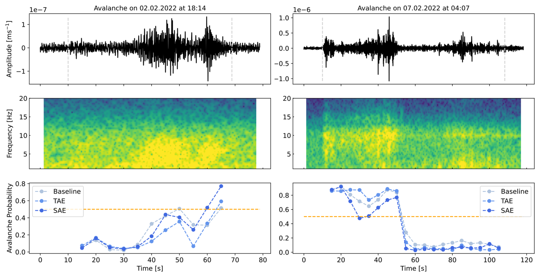
Figure 12Waveform and spectrogram generated by avalanches triggered on 2 February 2022 at 18:14 UTC (left) and 7 February 2022 at 04:07 (right). The signals have been filtered from 1 to 10 Hz corresponding to the input frequency band of the models. At the bottom, a comparison of the sensor array-based probabilities of each model over the entire length of the avalanche signal is shown. The manually defined event onset and end are highlighted in dashed grey lines (upper plot), and the classification threshold 0.5 is in orange (lower plot).
6.3 False alarms
The second type of error, i.e. false positives (FPs) or false alarms, showed greater variation in numbers across the three models. With 7.6 % (±0.1 %) (Fig. 8), the baseline produced the least amount of false positives. Predicting with the TAE features resulted in roughly twice as many false positives, with the SAE feature prediction in between. However, we observed a significant improvement in these errors when aggregating over the sensor array (Fig. 9). This suggested that the five recordings of some noise events showed substantial variations across the sensor array, which we filtered by this averaging. As the noise class is highly dominant (11135 windows) and, for instance, 10 % FPs result in approximately 1000 FP samples (compared to 1335 avalanche samples), the avalanche precision of all three models is relatively low with 0.52 (±0.00) (baseline), 0.33 (±0.01) (TAE) and 0.44 (±0.01) (SAE) (Table 1). We therefore analysed the origins of FPs to find potential tendencies or failure cases (Fig. 13). Most FPs, i.e. 77 % (baseline), 66 % (TAE) and 72 % (SAE), were generated by windows either carrying a non-zero avalanche score or belonging to an earthquake. Interestingly, the highest portion of false positives fell to windows with an avalanche score of 0.5, i.e. “one” expert thought it might be an avalanche. This could indicate that minor-size avalanches, or larger avalanches that flowed at the detection limits of the system, were not well recognised by the experts yet by the models. Considering the earthquakes, the test fold comprised a total of 3880 earthquake windows, of which only 132 (Seismic), 214 (TAE) and 146 (SAE) were misclassified as avalanches, i.e. 3.4 %, 5.5 % and 3.8 %. This underscored the earlier observation of good separation between avalanches and earthquakes in the latent spaces. The remaining approx. 30 % FPs in all models originated from unknown sources.
First, our results thus showed that using an array of sensors helped to reduce the number of false avalanche detections by averaging the single-sensor predictions. This can be viewed as model ensembling and is generally known to improve results (Mohammed and Kora, 2023). Second, including frequency domain features tended to show fewer FPs. Third, an interesting and positive finding was that the models rarely confused earthquakes for avalanches (on average 4.2 % of all earthquake windows). Moreover, the models generated false alerts to a similar extent to previous studies in avalanche detection (Bessason et al., 2007; Rubin et al., 2012; Hammer et al., 2017; Heck et al., 2018a). In pursuit of reducing the number of false alerts, one might consider including other types of recordings, e.g. infrasound data (Mayer et al., 2020). In addition, considering longer seismic windows in future implementations might help reduce the number of false alerts. However, this would require more avalanche data to start with and to train models.
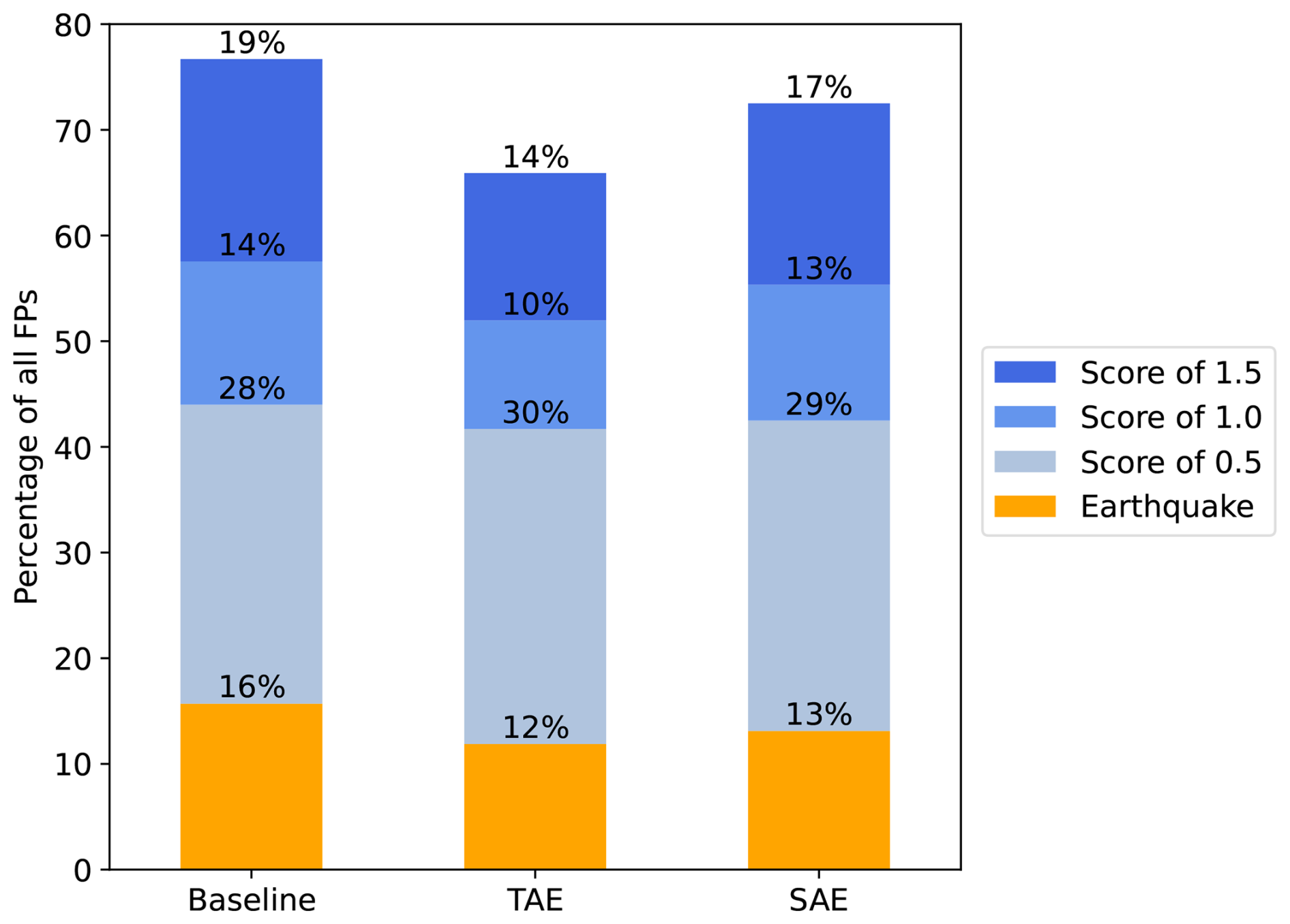
Figure 13Analysis of origins for false positives as a percentage of the total amount of false positives per model.
6.4 Applicability to early warning and monitoring systems
In a potential early-warning operation, a practical model must detect all key parts of the signal, particularly the onset, to identify avalanche movement in its early stages and trigger an appropriate alert. The current classifiers, which often failed to capture these avalanche onsets, may not yet be suitable for this purpose. To improve early-warning models, future studies should focus on examining avalanche onsets in more detail and developing specialised models that target these specific signal windows. For avalanche activity monitoring, false negatives at the start or end of each event are not very problematic. As long as the most energetic part of the signal is well detected, the overall avalanche activity can still be accurately recorded. However, when assessing overall avalanche activity, missed detections can be problematic. Therefore, we further post-processed the sensor array-based predictions (Fig. 9) to formulate event-based predictions (Sect. 5.3) and give a broader outlook. In theory, this should eliminate the FNs in the tails of the actual signal and provide us with event-based detectors. For instance, in Fig. 12, the models then would detect avalanches with this post-processing. And indeed, in Fig. E2, we observed a drastic reduction in missed avalanches for the three models, which achieved a high true positive rate of 81.4 % (±1.1 %) (baseline), 84.8 % (±2.6 %) (TAE) and 89.3 % (±4.3 %) (SAE).
In conclusion, we observed that the models struggled to detect the starting and ending of an event (Fig. 12). We argued that this behaviour was reasonable and, in part, desirable as these parts of an event often resemble background noise. However, in most cases, the entire (unique) event was detected (Fig. E2). Thus, the models could be implemented in an avalanche activity assessment process or to annotate large datasets in the future by being aware of their limitations and the fact that they tend to produce too many avalanche detections. Another compelling prerequisite for avalanche activity monitoring in future studies is the transferability to other study sites. We would expect variations in the detection performance to arise from different configurations in the study site setup, sensor location and configuration, and the characteristics of the terrain and the avalanches. Therefore, also implementing specialised data augmentation techniques to increase the variety and number of the avalanche recordings, e.g. seismic data augmentation techniques (Zhu et al., 2020) or generative models (Wang et al., 2021), might help to make the classifiers more robust to changing environments and setups.
6.5 Comparison to previous studies
To conclude, we put our results in a broader context by comparing them with previous studies. Provost et al. (2017) used a random forest model based on 71 engineered seismic attributes to classify landslides. They reported stunning true positive rates of 94 %, 93 % and 94 % for the rockfall, quake and earthquake class and a true negative rate of 92 % for the noise class. Therefore, we adopted their feature extraction approach as our baseline model, though our dataset differed significantly. They used non-windowed signals from an evenly distributed dataset comprising 418 rockfalls, 239 quakes, 407 earthquakes, and 395 noise events. Moreover, they included polarity and network attributes in the features, which for the classification turned out to be most important. However, with 92 % true negative rate, their model is comparably prone to producing FPs (false alerts) as the models in this study were. For avalanche detection, several studies also presented the approach of feature engineering and subsequent classification (Bessason et al., 2007; Rubin et al., 2012; Hammer et al., 2017; Heck et al., 2018a). Rubin et al. (2012) used 10 engineered features in the frequency domain and tested 12 classification models, of which the decision stump classifier showed the highest overall accuracy of 0.93. However, the model showed a poor precision of 0.13, producing many more false alerts compared to our classifiers. Heck et al. (2018a) used the same avalanche catalogue of 283 avalanches, of which 25 were confirmed and the rest were labelled by three experts. They implemented engineered temporal and spectral features and used an HMM as a classifier. Similar to most previous studies, they also noted high values of FPs. Moreover, they observed improvements when aggregating single-sensor to sensor array-based predictions as we did in this study. In conclusion, based on the results of this and previous studies, we expect that an avalanche predictor based on solely seismic data will always produce false alarms, as it remains a difficult task to identify low-energy avalanche signals. Therefore, installing a secondary seismic detection system near the avalanche path would be advantageous in mitigating false alarms. However, given the terrain characteristics at our study site (Fig. 1), where avalanches can occur along multiple paths, a single additional detection system may not be sufficient to detect all events. Alternatively, integrating a complementary detection system like an infrasound system could be beneficial but less cost-effective.
We proposed two autoencoder-based feature extractors and retrieved a set of standard engineered seismic attributes (Provost et al., 2017) to train three random forest classifiers for avalanche detection. We compiled and annotated a dataset from seismic avalanche data recorded during two winter seasons in Davos, Switzerland. While in earlier studies, seismic data classification mostly followed the approach of engineering well-defined signal attributes to train classifiers, the proposed autoencoder models bridged the gap to a purely learned (automatic) pipeline.
Overall, the classifiers achieved macro-average F1-scores ranging from 0.70 (±0.01) to 0.78 (±0.00) with avalanche recall values ranging from 0.67 (±0.00) to 0.71 (±0.02). Moreover, the results clearly suggested that including features from the frequency domain improves model performance. Further, as we observed that the models often misclassified the onset and end of avalanche signals but not the most energetic signal parts, we proposed a straightforward post-processing step. By imposing that at least two consecutive prediction windows, i.e. 15 s, must be positive for an entire event to be positive, we drastically reduced the missed avalanches (false negatives). This criterion significantly improved the avalanche recall, ranging from 0.81 (±0.01) to 0.89 (±0.04). Lastly, contrary to previous expectations, earthquakes were rarely mistaken for avalanches at our study site.
Revisiting the primary objective of advancing and automating avalanche detection through seismic monitoring systems, we believe that both the baseline implementation and the novel autoencoder-based approaches for avalanche data analysis bear strong potential for future implementations. We demonstrated that autoencoders can learn characteristic avalanche features from merely 84 seismic avalanche signals and are performing equally on an avalanche detection task as expert-engineered features, which have been studied and applied for over a decade, optimised and fine-tuned through various studies. Therefore, we argue that as seismic datasets grow, i.e. with more (diverse) avalanche signals available for learning, unsupervised representation learning methods could potentially surpass the conventional feature engineering approach in the future. In conclusion, the proposed methods represent a step towards enhancing the throughput of avalanche detection systems and the automatic and continuous documentation of events. Acquiring avalanche detections from such systems across different locations spanning wider areas has the potential to improve and validate avalanche warning services. This, however, necessitates future work on investigating the scalability and transferability of such methods to new environments.
Table A1Detailed view on the applied splits of the dataset. For each fold, the table shows the number of respective events. The folds were picked consecutive in time, with a minor exception in the test fold, which included the 2nd of February from fold 3. This balanced the number of events in the folds more evenly.
The implemented engineered feature extraction followed the work of Provost et al. (2017) and Turner et al. (2021). In contrast, by using bandpass-filtered signals (1–10 Hz), we modified the attributes correspondingly. Also, we discarded network and polarity-related attributes as we developed models for a single-sensor setting, and our study site only used one-component sensors. In summary, we extracted 22 waveform attributes (Table B1), 17 spectral (Table B2) and 18 spectrogram attributes (Table B3).
Table B1Waveform attributes extracted from the 10 s seismic signals.
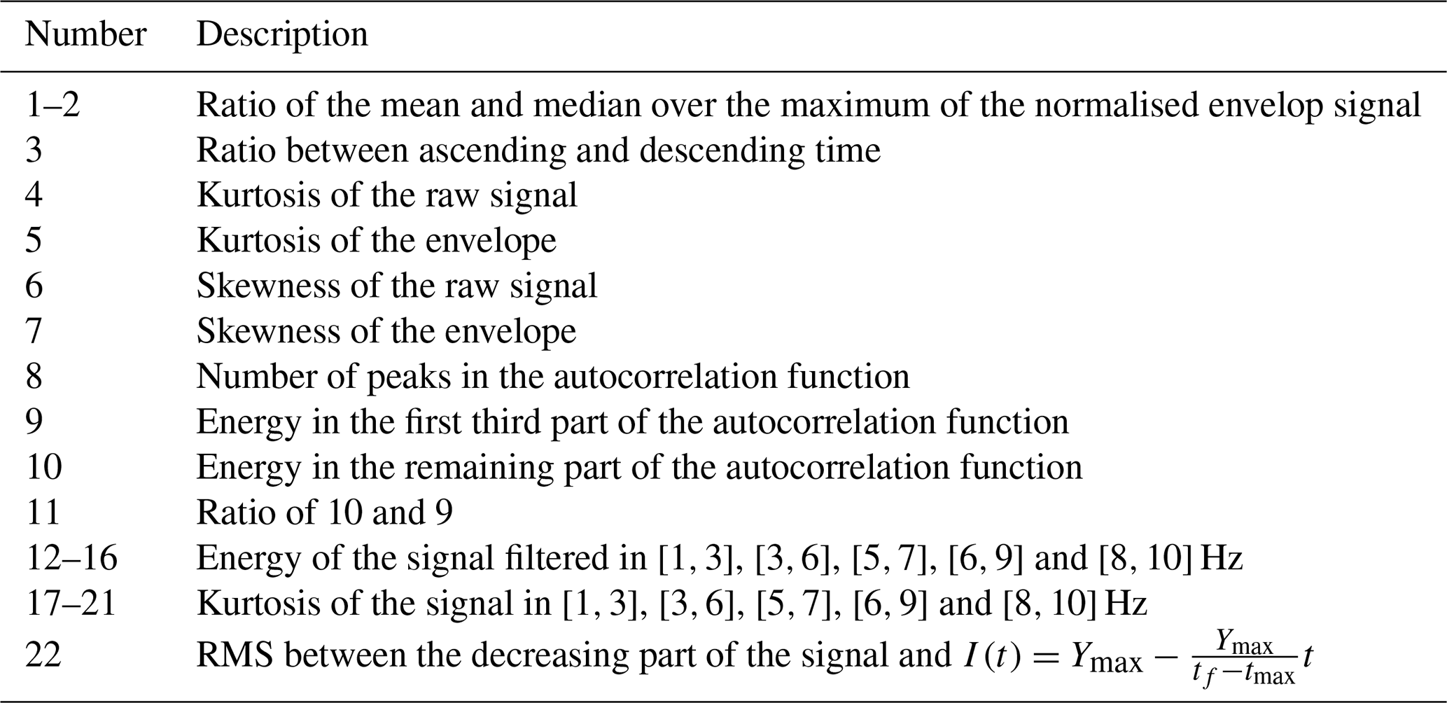
Table B2Spectral attributes extracted from the 10 s seismic signals.
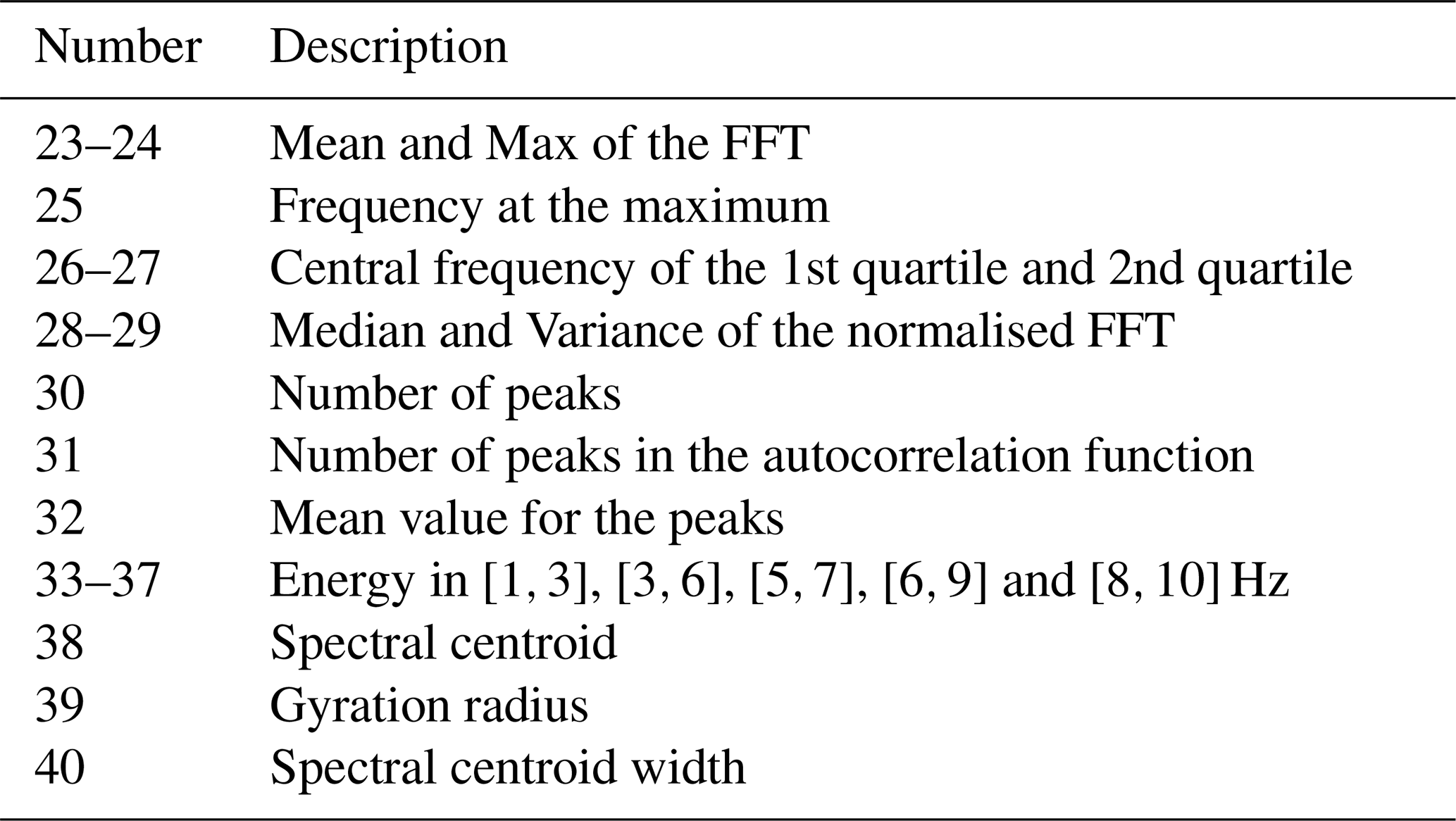
Table B3Spectrogram attributes extracted from the 10 s seismic signals.
We used the reconstruction, classification and clustering metrics defined here to evaluate the autoencoders and the classifiers.
C1 Reconstruction metrics
Since autoencoders aim at reconstructing a given input signal y, they are trained using a reconstruction loss. In this study, we implemented the mean squared error loss (MSE), which is defined for a batch of size B as follows.
is the autoencoder's predicted output, i.e., the reconstruction.
C2 Classification metrics
Various metrics exist to evaluate binary classification problems. All are tailored to specific objectives. For instance, the precision is chosen when false alerts, i.e. false positives, are critical, the recall is sensitive to missed events, i.e. false negatives, and the F1-score combines both to form the harmonic mean as follows:
The macro average summarises the per-class results within a single value. This value is an unweighted mean over the given classes and ensures that the values are not biased towards the majority class.
C3 Clustering metrics
A natural metric choice when evaluating autoencoders is the reconstruction loss, e.g. the mean squared error, on which we trained the autoencoders in this work. In pursuit of good autoencoder features for later classification, however, we aimed to optimise the latent space representation. Since a good reconstruction does not necessarily imply a sufficient separation in latent space, we explored clustering metrics to compare the latent space distribution of different models with the given (expert) labels. We, therefore, implemented the silhouette score (Rousseeuw, 1987) and the Calinski–Harabasz index (Caliński and Harabasz, 1974). These scores are usually used to evaluate clustering algorithms that predict classes, e.g. k-means. The silhouette score computes the mean intra-cluster and inter-cluster distances per sample. For instance, given a sample, it calculates the distance to the cluster it is part of (a) and the distance to the nearest cluster it is not part of (b) and forms the sample score:
After taking the mean over all samples, the silhouette score ranges from −1 (worst) to 1 (best). The Calinski–Harabasz index, or variance ratio criterion, on the other hand, is the ratio of between- and within-cluster dispersion. The between-cluster dispersion is defined as the weighted sum of squared Euclidean distances of the cluster centroids and the overall centroid (higher better). The within-cluster dispersion is given as the sum of the squared Euclidean distance of the samples and their respective cluster centre (lower better). Thus, a good clustering algorithm is supposed to yield a high Calinski–Harabasz score.
To select the autoencoder hyper-parameters, we opted first to optimise model intrinsic parameters, such as hidden dimensions or the number of layers, instead of training strategy parameters. This separation reduced the computation time.
The temporal autoencoder architecture optimisation proved to be more sensitive and critical. First, we optimised the kernel size, stride, number of filters, feature dimension and activation function. We observed that the kernel size and stride combinations of (20, 10) and (8, 4) showed the best clustering metrics. Moreover, concerning the non-linear activation, the leaky ReLU outperformed the Tanh function in most tests. Since the overall performance was not satisfying, we tested the weighted random sampler (Sect. 4.2.2 with 50 % expected avalanches in each batch. This addition to the training strategy showed a considerable improvement for most models with kernel size 20 and stride 10. Although using a kernel size of 8 and stride of 4 tended to show better clustering metrics, the reconstruction of the signals was comparably poor. Based on these observations, we implemented a kernel size of 20 and stride of 10. Also, we found the feature dimension 32 better suited than 64 or 16. Lastly, we selected 32, 64, and 128 filters within each encoder layer. See Table E2 for a summary of the best 10 models of this process and Table E1 for the selected autoencoders. Having defined the intrinsic parameters, we tested different training strategies. In particular, we optimised the learning rate, the batch size and the expected portion of avalanches per batch. This test led to values of , 128 and 0.6 for the temporal autoencoder (Table E3). Finally, we found that augmenting the data by randomly shifting input samples by 0 to 1 s to the left or right improved robustness.
While optimising the spectral autoencoder, we found faster convergence. We started by testing combinations of the number of layers with hidden dimensions, feature dimensions and activation functions. Table E4 shows the results for the best eight models. We foremost noted that 16 features were optimal for this task. Moreover, we observed that the Tanh activation function was favourable in comparable architectures. Finally, we selected the model highlighted in bold since it showed a good compromise between the number of weights in the network and performance. Following the same training strategy as for the temporal autoencoder, we optimised the learning rate, the batch size and the expected portion of avalanches per batch. In contrast to the temporal autoencoder, we used an expected portion of 0.5 avalanches within a batch, a learning rate of and a batch size of 128 (Table E5).
Table E2Summary of the TAE hyper-parameter optimisation. Only the models for which all three metrics are ranked in the top 20 are shown. The best metrics and the selected model are highlighted in bold.
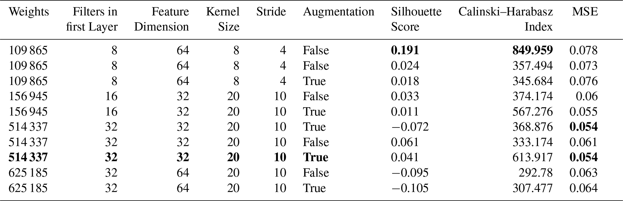
Table E3Summary of the TAE learning rate and batch size optimisation. The best metrics and the selected model are highlighted in bold.
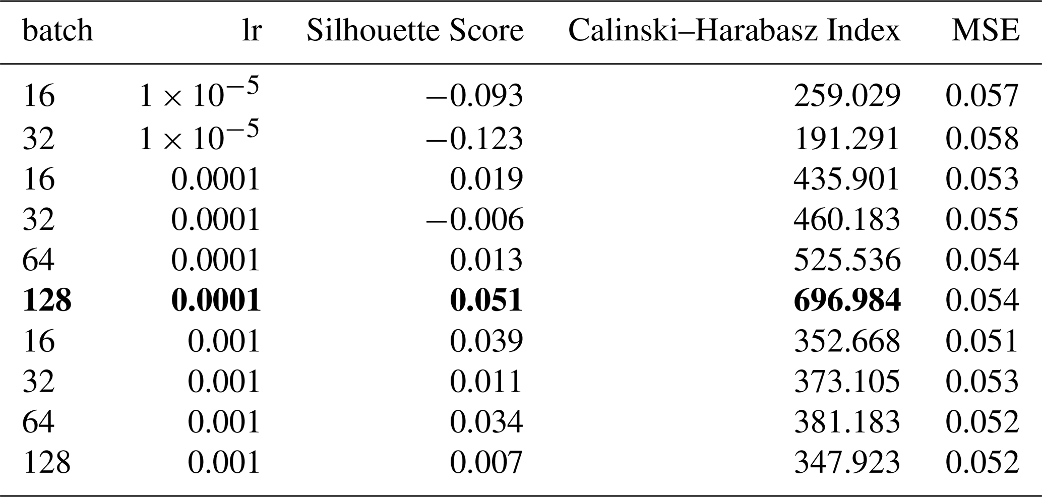
Table E4Summary of the SAE hyper-parameter optimisation. Only the models for which all three metrics are ranked in the top 10 are shown. A “default” hidden dimension indicates that the dimensions in the layers of the encoder linearly decrease from the input dimension (200) to the feature dimension. The best clustering metrics and the selected model are highlighted in bold.
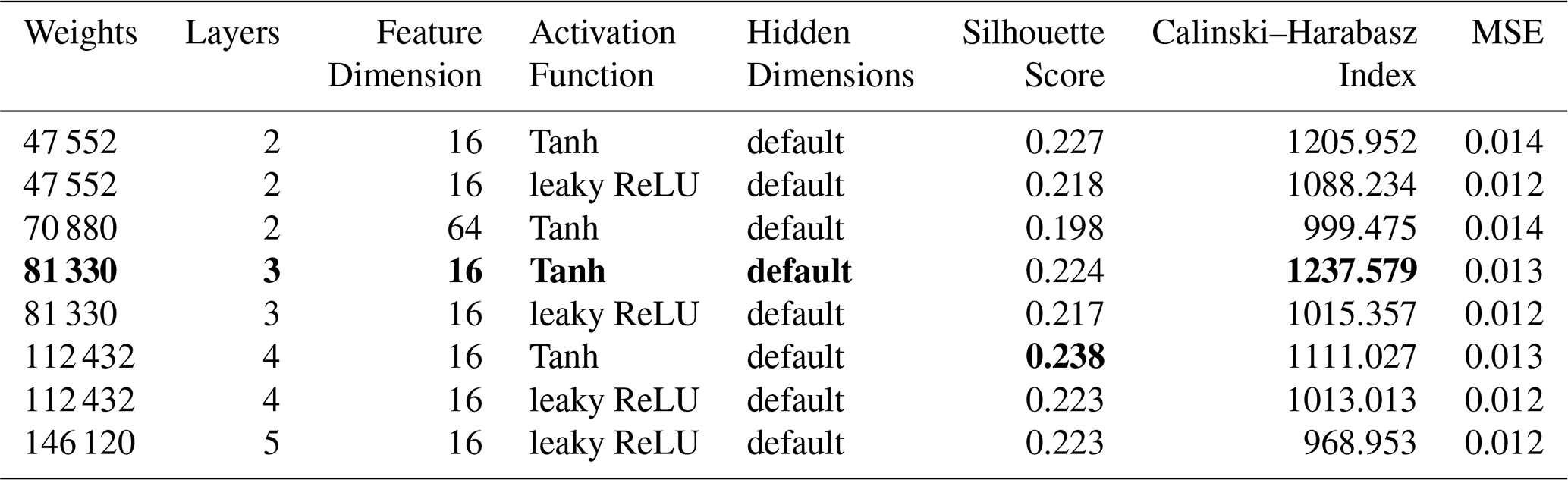
Table E5Summary of the SAE learning rate and batch size optimisation. Only the top ten models are shown. The best clustering metrics and the selected model are highlighted in bold.
E1 Learning curves
E2 Event-based prediction results
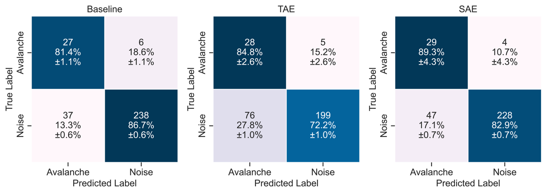
Figure E2Confusion matrices of the results for the three feature sets aggregated on event level. The rows indicate the true (expert) labels, while the columns provide the predicted labels of the random forest classifiers. The colours code the percentage numbers.
Table E6Classification metrics on the (unseen) test fold data comprising 33 avalanche and 275 noise samples after the aggregation over entire events of the sensor array-based predictions. Due to the strong class imbalance and bias towards the noise class, the weighted averages of the metrics are not shown.
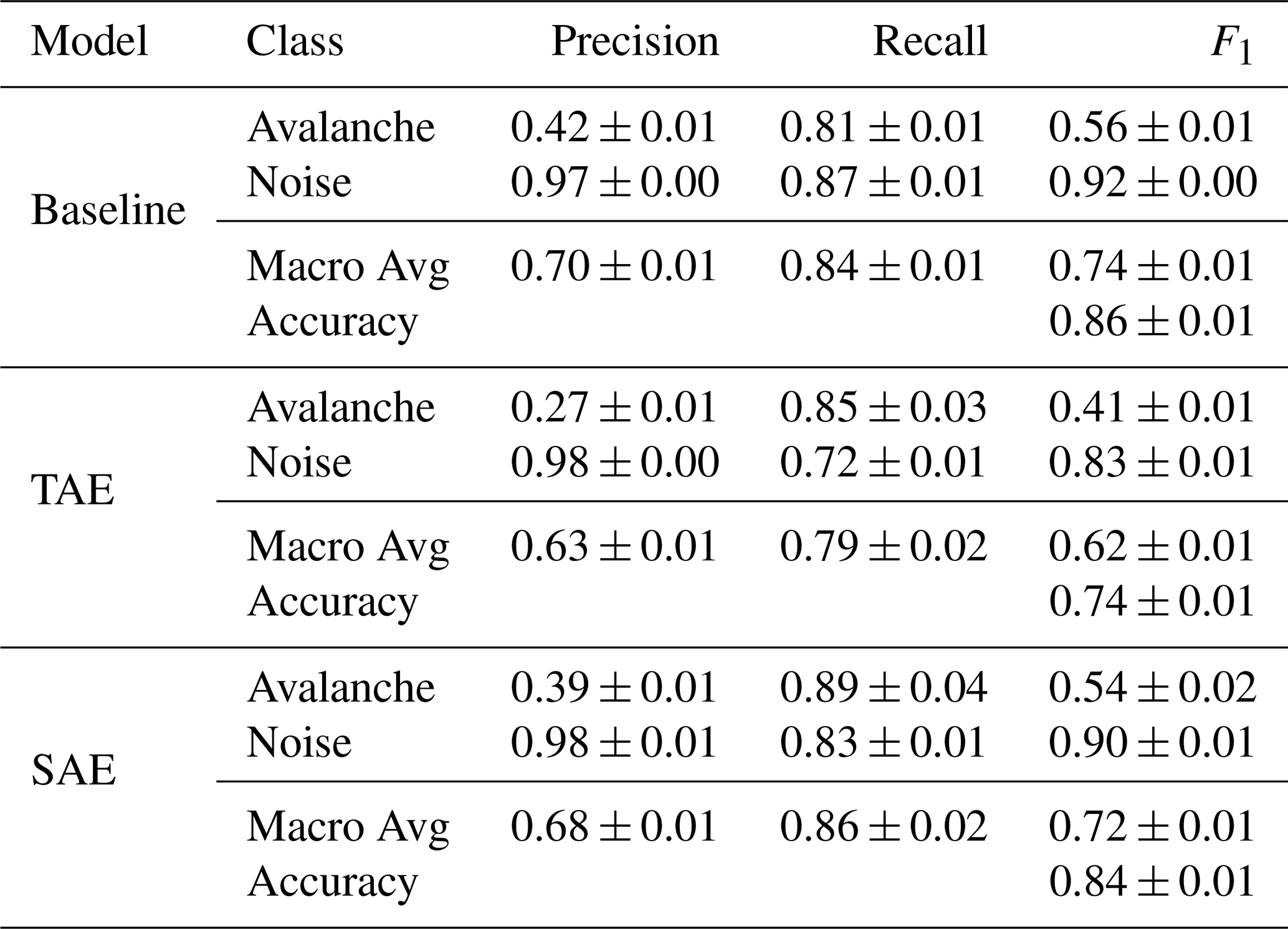
The code to reproduce the results and test the models is available on Zenodo (Simeon, 2025, https://doi.org/10.5281/zenodo.15001358). It is predominately written in Python using the PyTorch library (Paszke et al., 2019) for the autoencoder design, the random forest implementation of the Scikit-learn library (Pedregosa et al., 2011), the Pandas library (McKinney, 2010) for handling the data and more standard Python libraries such as NumPy (Harris et al., 2020) and SciPy (Virtanen et al., 2020). Additionally, the event catalogue with the raw seismic waveforms is found on Zenodo (Simeon et al., 2025, https://doi.org/10.5281/zenodo.14892926).
AS: concept and design of the study, data collection and curation, model development, computational framework, analysis, writing, CP: concept and design of the study, data collection and curation, model development, computational framework, analysis, writing, reviewing, MV: concept and design of the study, model development, analysis, reviewing, CS: data collection and curation, computational framework, reviewing, AH: concept and design of the study, data collection and curation, analysis, reviewing
The contact author has declared that none of the authors has any competing interests.
Publisher’s note: Copernicus Publications remains neutral with regard to jurisdictional claims made in the text, published maps, institutional affiliations, or any other geographical representation in this paper. While Copernicus Publications makes every effort to include appropriate place names, the final responsibility lies with the authors. Views expressed in the text are those of the authors and do not necessarily reflect the views of the publisher.
This study was supported by a grant from the Innosuisse – Swiss Innovation Agency (37619.1 IP-ENG). We thank Fernando Pérez-Cruz for the helpful discussions and numerous colleagues from SLF for help with fieldwork and maintaining the instrumentation. We thank Geoprevent, and in particular Lino Schmid and Johannes Gassner, for sharing the radar data with us and helping with the interpretation.
This research has been supported by the Innosuisse – Schweizerische Agentur für Innovationsförderung (grant no. 37619.1 IP-ENG).
This paper was edited by Le Yu and reviewed by Tate Meehan, Kevin Hank, and four anonymous referees.
Barandas, M., Folgado, D., Fernandes, L., Santos, S., Abreu, M., Bota, P., Liu, H., Schultz, T., and Gamboa, H.: TSFEL: Time Series Feature Extraction Library, SoftwareX, 11, 100456, https://doi.org/10.1016/j.softx.2020.100456, 2020. a
Bengio, Y., Courville, A., and Vincent, P.: Representation Learning: A Review and New Perspectives, IEEE Transactions on Pattern Analysis and Machine Intelligence, 35, 1798–1828, https://doi.org/10.1109/TPAMI.2013.50, 2013. a, b
Bessason, B., Eiríksson, G., Thórarinsson, Ó., Thórarinsson, A., and Einarsson, S.: Automatic detection of avalanches and debris flows by seismic methods, J. Glaciol., 53, 461–472, https://doi.org/10.3189/002214307783258468, 2007. a, b, c
Biescas, B., Dufour, F., Furdada, G., Khazaradze, G., and Suriñach, E.: Frequency content evolution of snow avalanche seismic signals, Surv. Geophys., 24, 447–464, https://doi.org/10.1023/B:GEOP.0000006076.38174.31, 2003. a
Breiman, L.: Random Forests, Machine Learning, 45, 5–32, https://doi.org/10.1023/A:1010933404324, 2001. a
Breiman, L.: Classification and regression trees, Routledge, https://doi.org/10.1201/9781315139470, 2017. a
Bründl, M., Etter, H.-J., Steiniger, M., Klingler, Ch., Rhyner, J., and Ammann, W. J.: IFKIS – a basis for managing avalanche risk in settlements and on roads in Switzerland, Nat. Hazards Earth Syst. Sci., 4, 257–262, https://doi.org/10.5194/nhess-4-257-2004, 2004. a
Bühler, Y., Bebi, P., Christen, M., Margreth, S., Stoffel, L., Stoffel, A., Marty, C., Schmucki, G., Caviezel, A., Kühne, R., Wohlwend, S., and Bartelt, P.: Automated avalanche hazard indication mapping on a statewide scale, Nat. Hazards Earth Syst. Sci., 22, 1825–1843, https://doi.org/10.5194/nhess-22-1825-2022, 2022. a, b
Caliński, T. and Harabasz, J.: A dendrite method for cluster analysis, Communications in Statistics, 3, 1–27, https://doi.org/10.1080/03610927408827101, 1974. a, b
Chmiel, M., Walter, F., Wenner, M., Zhang, Z., McArdell, B. W., and Hibert, C.: Machine Learning Improves Debris Flow Warning, Geophysical Research Letters, 48, https://doi.org/10.1029/2020GL090874, 2021. a, b
Clinton, J., Cauzzi, C., Fäh, D., Michel, C., Zweifel, P., Olivieri, M., Cua, G., Haslinger, F., and Giardini, D.: The Current State of Strong Motion Monitoring in Switzerland, Springer Netherlands, 219–233, ISBN 978-94-007-0152-6, https://doi.org/10.1007/978-94-007-0152-6_15, 2011. a
Dammeier, F., Moore, J. R., Hammer, C., Haslinger, F., and Loew, S.: Automatic detection of alpine rockslides in continuous seismic data using hidden Markov models, Journal of Geophysical Research: Earth Surface, 121, 351–371, https://doi.org/10.1002/2015JF003647, 2016. a
EAWS: European Avalanche Size Scale, https://www.avalanches.org/standards/avalanche-size/ (last access: 3 September 2024), 2021. a
EMSC-CSEM: Euro-Mediterranean Seismological Centre (EMSC), https://www.emsc-csem.org/#2 (last access: May 2023), 2023. a
Gu, S., Kelly, B., and Xiu, D.: Autoencoder asset pricing models, Journal of Econometrics, 222, 429–450, https://doi.org/10.1016/j.jeconom.2020.07.009, 2021. a
Hammer, C., Ohrnberger, M., and Fäh, D.: Classifying seismic waveforms from scratch: a case study in the alpine environment, Geophysical Journal International, 192, 425–439, https://doi.org/10.1093/gji/ggs036, 2013. a
Hammer, C., Fäh, D., and Ohrnberger, M.: Automatic detection of wet-snow avalanche seismic signals, Natural Hazards, 86, 601–618, https://doi.org/10.1007/s11069-016-2707-0, 2017. a, b, c, d, e
Harris, C. R., Millman, K. J., van der Walt, S. J., Gommers, R., Virtanen, P., Cournapeau, D., Wieser, E., Taylor, J., Berg, S., Smith, N. J., Kern, R., Picus, M., Hoyer, S., van Kerkwijk, M. H., Brett, M., Haldane, A., del Río, J. F., Wiebe, M., Peterson, P., Gérard-Marchant, P., Sheppard, K., Reddy, T., Weckesser, W., Abbasi, H., Gohlke, C., and Oliphant, T. E.: Array programming with NumPy, Nature, 585, 357–362, https://doi.org/10.1038/s41586-020-2649-2, 2020. a
Heck, M., Hammer, C., van Herwijnen, A., Schweizer, J., and Fäh, D.: Automatic detection of snow avalanches in continuous seismic data using hidden Markov models, Nat. Hazards Earth Syst. Sci., 18, 383–396, https://doi.org/10.5194/nhess-18-383-2018, 2018a. a, b, c, d
Heck, M., Hobiger, M., van Herwijnen, A., Schweizer, J., and Fäh, D.: Localization of seismic events produced by avalanches using multiple signal classification, Geophysical Journal International, 216, 201–217, https://doi.org/10.1093/gji/ggy394, 2018b. a, b, c, d, e
Heck, M., van Herwijnen, A., Hammer, C., Hobiger, M., Schweizer, J., and Fäh, D.: Automatic detection of avalanches combining array classification and localization, Earth Surf. Dynam., 7, 491–503, https://doi.org/10.5194/esurf-7-491-2019, 2019. a
Hendrick, M., Techel, F., Volpi, M., Olevski, T., Pérez-Guillén, C., van Herwijnen, A., and Schweizer, J.: Automated prediction of wet-snow avalanche activity in the Swiss Alps, Journal of Glaciology, 1–14, https://doi.org/10.1017/jog.2023.24, 2023. a
Hibert, C., Mangeney, A., Grandjean, G., Baillard, C., Rivet, D., Shapiro, N. M., Satriano, C., Maggi, A., Boissier, P., Ferrazzini, V., and Crawford, W.: Automated identification, location, and volume estimation of rockfalls at Piton de la Fournaise volcano, Journal of Geophysical Research: Earth Surface, 119, 1082–1105, https://doi.org/10.1002/2013JF002970, 2014. a
Hinton, G. E. and Salakhutdinov, R. R.: Reducing the Dimensionality of Data with Neural Networks, Science, 313, 504–507, https://doi.org/10.1126/science.1127647, 2006. a
Hochreiter, S. and Schmidhuber, J.: Long Short-Term Memory, Neural Comput., 9, 1735–1780, https://doi.org/10.1162/neco.1997.9.8.1735, 1997. a
Ioffe, S. and Szegedy, C.: Batch Normalization: Accelerating Deep Network Training by Reducing Internal Covariate Shift, CoRR, arXiv [preprint], https://doi.org/10.48550/arXiv.1502.03167, 2015. a
Ismail Fawaz, H., Forestier, G., Weber, J., Idoumghar, L., and Muller, P.-A.: Deep learning for time series classification: a review, Data Mining and Knowledge Discovery, 33, 917–963, https://doi.org/10.1007/s10618-019-00619-1, 2019. a
Kingma, D. P. and Ba, J.: Adam: A Method for Stochastic Optimization, arXiv [preprint], https://doi.org/10.48550/arXiv.1412.6980, 2014. a
Kiranyaz, S., Avci, O., Abdeljaber, O., Ince, T., Gabbouj, M., and Inman, D. J.: 1D convolutional neural networks and applications: A survey, Mechanical Systems and Signal Processing, 151, 107398, https://doi.org/10.1016/j.ymssp.2020.107398, 2021. a
Kong, Q., Chiang, A., Aguiar, A. C., Fernández-Godino, M. G., Myers, S. C., and Lucas, D. D.: Deep convolutional autoencoders as generic feature extractors in seismological applications, Artificial Intelligence in Geosciences, 2, 96–106, https://doi.org/10.1016/j.aiig.2021.12.002, 2021. a
Lacroix, P., Grasso, J. R., Roulle, J., Giraud, G., Goetz, D., Morin, S., and Helmstetter, A.: Monitoring of snow avalanches using a seismic array: Location, speed estimation, and relationships to meteorological variables, J. Geophys. Res.-Earth, 117, 1–15, https://doi.org/10.1029/2011JF002106, 2012. a, b, c
Längkvist, M., Karlsson, L., and Loutfi, A.: A review of unsupervised feature learning and deep learning for time-series modeling, Pattern Recognition Letters, 42, 11–24, https://doi.org/10.1016/j.patrec.2014.01.008, 2014. a, b
Leprettre, B., Navarre, J.-P., Taillefer, A., Danielou, Y., organisms Panel, J. T. M., and Touvier, F.: Reliable Estimation of Avalanche Activity Using Seismic Methods, https://api.semanticscholar.org/CorpusID:54986472 (last access: March 2024), 1996. a
Li, Z., Meier, M. A., Hauksson, E., Zhan, Z., and Andrews, J.: Machine Learning Seismic Wave Discrimination: Application to Earthquake Early Warning, Geophysical Research Letters, 45, 4773–4779, https://doi.org/10.1029/2018GL077870, 2018. a
Lima, F. T. and Souza, V. M.: A Large Comparison of Normalization Methods on Time Series, Big Data Research, 34, 100407, https://doi.org/10.1016/j.bdr.2023.100407, 2023. a
Lin, G. W., Hung, C., Chien, Y. F. C., Chu, C. R., Liu, C. H., Chang, C. H., and Chen, H.: Towards automatic landslide-quake identification using a random forest classifier, Applied Sciences (Switzerland), 10, https://doi.org/10.3390/app10113670, 2020. a
Marchetti, E., Ripepe, M., Ulivieri, G., and Kogelnig, A.: Infrasound array criteria for automatic detection and front velocity estimation of snow avalanches: towards a real-time early-warning system, Nat. Hazards Earth Syst. Sci., 15, 2545–2555, https://doi.org/10.5194/nhess-15-2545-2015, 2015. a
Mayer, S., van Herwijnen, A., Ulivieri, G., and Schweizer, J.: Evaluating the performance of an operational infrasound avalanche detection system at three locations in the Swiss Alps during two winter seasons, Cold regions science and technology, 173, 102962, https://doi.org/10.1016/j.coldregions.2019.102962, 2020. a
Mayer, S., Techel, F., Schweizer, J., and van Herwijnen, A.: Prediction of natural dry-snow avalanche activity using physics-based snowpack simulations, Nat. Hazards Earth Syst. Sci., 23, 3445–3465, https://doi.org/10.5194/nhess-23-3445-2023, 2023. a
McClung, D. and Schaerer, P. A.: The avalanche handbook, The Mountaineers Books, ISBN 978-1-68051-539-8, 2006. a
McKinney, W.: Data Structures for Statistical Computing in Python, in: Proceedings of the 9th Python in Science Conference, edited by: van der Walt, S. and Millman, J., 56–61, https://doi.org/10.25080/Majora-92bf1922-00a, 2010. a
Meier, L., Jacquemart, M., Blattmann, B., and Arnold, B.: Real-time avalanche detection with long-range, wide-angle radars for road safety in Zermatt, Switzerland, in: Proceedings of the International Snow Science Workshop, Breckenridge, CO, 304–308, https://api.semanticscholar.org/CorpusID:59408658 (last access: March 2024), 2016. a
Mohammed, A. and Kora, R.: A comprehensive review on ensemble deep learning: Opportunities and challenges, Journal of King Saud University – Computer and Information Sciences, 35, 757–774, https://doi.org/10.1016/j.jksuci.2023.01.014, 2023. a
Mousavi, S. M. and Beroza, G. C.: Deep-learning seismology, Science, 377, eabm4470, https://doi.org/10.1126/science.abm4470, 2022. a
Mousavi, S. M., Zhu, W., Ellsworth, W., and Beroza, G.: Unsupervised Clustering of Seismic Signals Using Deep Convolutional Autoencoders, IEEE Geoscience and Remote Sensing Letters, 16, 1693–1697, https://doi.org/10.1109/LGRS.2019.2909218, 2019. a, b
Paszke, A., Gross, S., Massa, F., Lerer, A., Bradbury, J., Chanan, G., Killeen, T., Lin, Z., Gimelshein, N., Antiga, L., Desmaison, A., Köpf, A., Yang, E., DeVito, Z., Raison, M., Tejani, A., Chilamkurthy, S., Steiner, B., Fang, L., Bai, J., and Chintala, S.: PyTorch: An Imperative Style, High-Performance Deep Learning Library, arXiv [preprint], https://doi.org/10.48550/arXiv.1912.01703, 2019. a, b
Pedregosa, F., Varoquaux, G., Gramfort, A., Michel, V., Thirion, B., Grisel, O., Blondel, M., Prettenhofer, P., Weiss, R., Dubourg, V., Vanderplas, J., Passos, A., Cournapeau, D., Brucher, M., Perrot, M., and Duchesnay, E.: Scikit-learn: Machine Learning in Python, Journal of Machine Learning Research, 12, 2825–2830, https://doi.org/10.5555/1953048.2078195, 2011. a
Pérez-Guillén, C., Sovilla, B., Suriñach, E., Tapia, M., and Köhler, A.: Deducing avalanche size and flow regimes from seismic measurements, Cold Regions Science and Technology, 121, 25–41, https://doi.org/10.1016/j.coldregions.2015.10.004, 2016. a, b, c, d
Pérez-Guillén, C., Tsunematsu, K., Nishimura, K., and Issler, D.: Seismic location and tracking of snow avalanches and slush flows on Mt. Fuji, Japan, Earth Surf. Dynam., 7, 989–1007, https://doi.org/10.5194/esurf-7-989-2019, 2019. a, b, c
Provost, F., Hibert, C., and Malet, J. P.: Automatic classification of endogenous landslide seismicity using the Random Forest supervised classifier, Geophysical Research Letters, 44, 113–120, https://doi.org/10.1002/2016GL070709, 2017. a, b, c, d, e, f, g
Rakthanmanon, T., Campana, B., Mueen, A., Batista, G., Westover, B., Zhu, Q., Zakaria, J., and Keogh, E.: Searching and mining trillions of time series subsequences under dynamic time warping, in: Proceedings of the 18th ACM SIGKDD International Conference on Knowledge Discovery and Data Mining, KDD '12, Association for Computing Machinery, New York, NY, USA, 262–270, ISBN 9781450314626, https://doi.org/10.1145/2339530.2339576, 2012. a
Rousseeuw, P. J.: Silhouettes: A graphical aid to the interpretation and validation of cluster analysis, Journal of Computational and Applied Mathematics, 20, 53–65, https://doi.org/10.1016/0377-0427(87)90125-7, 1987. a, b
Rubin, M. J., Camp, T., Herwijnen, A. V., and Schweizer, J.: Automatically detecting avalanche events in passive seismic data, 1, 13–20, ISBN 9780769549132, https://doi.org/10.1109/ICMLA.2012.12, 2012. a, b, c, d, e
Rumelhart, D. E., Hinton, G. E., and Williams, R. J.: Learning internal representations by error propagation, MIT Press, Cambridge, MA, USA, 318–362, ISBN 026268053X, 1986. a, b
Schimmel, A., Hübl, J., Koschuch, R., and Reiweger, I.: Automatic detection of avalanches: evaluation of three different approaches, Natural Hazards, 87, https://doi.org/10.1007/s11069-017-2754-1, 2017. a
Schweizer, J., Mitterer, C., Techel, F., Stoffel, A., and Reuter, B.: On the relation between avalanche occurrence and avalanche danger level, The Cryosphere, 14, 737–750, https://doi.org/10.5194/tc-14-737-2020, 2020. a, b
Swiss Seismological Center (SED) at ETH Zurich: National Seismic Networks of Switzerland, http://www.seismo.ethz.ch/de/home/ (last access: May 2023), 2023. a
Seydoux, L., Balestriero, R., Poli, P., Hoop, M. D., Campillo, M., and Baraniuk, R.: Clustering earthquake signals and background noises in continuous seismic data with unsupervised deep learning, Nature Communications, 11, https://doi.org/10.1038/s41467-020-17841-x, 2020. a
Sielenou, P. D., Viallon-Galinier, L., Hagenmuller, P., Naveau, P., Morin, S., Dumont, M., Verfaillie, D., and Eckert, N.: Combining random forests and class-balancing to discriminate between three classes of avalanche activity in the French Alps, Cold Regions Science and Technology, 187, 103276, https://doi.org/10.1016/j.coldregions.2021.103276, 2021. a
Simeon, A.: Autoencoder-based feature extraction for the automatic detection of snow avalanches in seismic data, Zenodo [code], https://doi.org/10.5281/zenodo.15001358, 2025. a
Simeon, A., Seupel, C., Pérez-Guillén, C., and van Herwijnen, A.: Seismic Avalanche Signals recorded in Dischma Valley above Davos, Switzerland, Zenodo [data set], https://doi.org/10.5281/zenodo.14892926, 2025. a
Sola, J. and Sevilla, J.: Importance of input data normalization for the application of neural networks to complex industrial problems, IEEE Transactions on Nuclear Science, 44, 1464–1468, https://doi.org/10.1109/23.589532, 1997. a, b
Suriñach, E., Furdada, G., Sabot, F., Biescas, B., and Vilaplana, J.: On the characterization of seismic signals generated by snow avalanches for monitoring purposes, Ann. Glaciol., 32, 268–274, https://doi.org/10.3189/172756401781819634, 2001. a, b
Suriñach, E., Vilajosana, I., Khazaradze, G., Biescas, B., Furdada, G., and Vilaplana, J. M.: Seismic detection and characterization of landslides and other mass movements, Nat. Hazards Earth Syst. Sci., 5, 791–798, https://doi.org/10.5194/nhess-5-791-2005, 2005. a
Techel, F., Jarry, F., Kronthaler, G., Mitterer, S., Nairz, P., Pavšek, M., Valt, M., and Darms, G.: Avalanche fatalities in the European Alps: long-term trends and statistics, Geogr. Helv., 71, 147–159, https://doi.org/10.5194/gh-71-147-2016, 2016. a
Turner, R. J., Latto, R. B., and Reading, A. M.: An ObsPy Library for Event Detection and Seismic Attribute Calculation: Preparing Waveforms for Automated Analysis, Journal of Open Research Software, https://doi.org/10.5334/jors.365, 2021. a
van Herwijnen, A. and Schweizer, J.: Monitoring avalanche activity using a seismic sensor, Cold Regions Science and Technology,, 69, 165–176, https://doi.org/10.1016/j.coldregions.2011.06.008, 2011. a, b, c
van Herwijnen, A., Heck, M., and Schweizer, J.: Forecasting snow avalanches using avalanche activity data obtained through seismic monitoring, Cold Regions Science and Technology, 132, 68–80, https://doi.org/10.1016/j.coldregions.2016.09.014, 2016. a
van Herwijnen, A., Heck, M., Richter, B., Sovilla, B., and Techel, F.: When do avalanches release: investigating time scales in avalanche formation, in: International snow science workshop proceedings 2018, ISSW, Innsbruck, Austria, https://www.dora.lib4ri.ch/wsl/islandora/object/wsl:18935 (last access: March 2024), 2018. a
Vilajosana, I., Khazaradze, G., Suriñach, E., Lied, E., and Kristensen, K.: Snow avalanche speed determination using seismic methods, Cold Regions Science and Technology, 49, 2–10, https://doi.org/10.1016/j.coldregions.2006.09.007, 2007. a
Virtanen, P., Gommers, R., Oliphant, T. E., Haberland, M., Reddy, T., Cournapeau, D., Burovski, E., Peterson, P., Weckesser, W., Bright, J., van der Walt, S. J., Brett, M., Wilson, J., Millman, K. J., Mayorov, N., Nelson, A. R. J., Jones, E., Kern, R., Larson, E., Carey, C. J., Polat, İ., Feng, Y., Moore, E. W., VanderPlas, J., Laxalde, D., Perktold, J., Cimrman, R., Henriksen, I., Quintero, E. A., Harris, C. R., Archibald, A. M., Ribeiro, A. H., Pedregosa, F., van Mulbregt, P., and SciPy 1.0 Contributors: SciPy 1.0: Fundamental Algorithms for Scientific Computing in Python, Nature Methods, 17, 261–272, https://doi.org/10.1038/s41592-019-0686-2, 2020. a
Wang, T., Trugman, D., and Lin, Y.: SeismoGen: Seismic Waveform Synthesis Using GAN With Application to Seismic Data Augmentation, Journal of Geophysical Research: Solid Earth, 126, e2020JB020077, https://doi.org/10.1029/2020JB020077, 2021. a
Wenner, M., Hibert, C., van Herwijnen, A., Meier, L., and Walter, F.: Near-real-time automated classification of seismic signals of slope failures with continuous random forests, Nat. Hazards Earth Syst. Sci., 21, 339–361, https://doi.org/10.5194/nhess-21-339-2021, 2021. a
Xu, B., Wang, N., Chen, T., and Li, M.: Empirical Evaluation of Rectified Activations in Convolutional Network, arXiv [preprint], https://doi.org/10.48550/arXiv.1505.00853, 2015. a
Xugang, L., Yu, T., Shigeki, M., and Chiori, H.: Speech Enhancement Based on Deep Denoising Autoencoder, arXiv [preprint], https://doi.org/10.48550/arXiv.2001.01538, 2013. a
Zhu, W., Mousavi, S. M., and Beroza, G. C.: Chapter Four – Seismic signal augmentation to improve generalization of deep neural networks, in: Machine Learning in Geosciences, edited by: Moseley, B. and Krischer, L., Advances in Geophysics, Elsevier, 61 151–177, https://doi.org/10.1016/bs.agph.2020.07.003, 2020. a, b
- Abstract
- Introduction
- Study site and instrumentation
- Data
- Model development
- Results
- Discussion
- Conclusions
- Appendix A: Dataset
- Appendix B: Seismic attributes
- Appendix C: Metrics
- Appendix D: Random forest optimisation
- Appendix E: Autoencoder optimisation
- Code and data availability
- Author contributions
- Competing interests
- Disclaimer
- Acknowledgements
- Financial support
- Review statement
- References