the Creative Commons Attribution 4.0 License.
the Creative Commons Attribution 4.0 License.
 | 20 Nov 2025
On the proper use of screen-level temperature measurements in weather forecasting models over mountains
Danaé Préaux
Ingrid Dombrowski-Etchevers
Isabelle Gouttevin
Yann Seity
The near-surface air temperature, considered to be measured at about 2 m above the ground, is a key meteorological parameter with a wealth of uses for humankind. However, its accurate estimation in mountain regions is impeded by persistent limits inherent to atmospheric modeling over complex terrain. In the present study, we analyze the role of structural inhomogeneities of the valleys and mountains observational network in France to highlight their contribution to the misrepresentation of near-surface air temperature over mountain regions in the numerical weather prediction (NWP) system Arome-France. We examine in particular the effects of the disparity in height above ground of the temperature measurements, of the inhomogeneous geographical distribution of stations that are preferentially located in valleys, and of the relief mismatch between station location and model grid points. The consequences of these inhomogeneities are analyzed through their effect on model performance evaluation and on the assimilation, with a focus on the winter season. In France, high-altitude stations usually measure temperature at about 7 m over the snow-free ground and on average 1 to 2 m lower when the ground is snow-covered in winter. We show that this height difference with respect to standard stations measuring at 2 m should be considered both when evaluating the model performances and in assimilation. In terms of scores, model behaviors can be highly different at 2 m vs. 5 m so that confounding the two levels can lead to a strong mischaracterization of model biases. This confusion additionally makes the assimilation of high-altitude stations detrimental to the analysis for the Arome-France NWP system. We also show that due to the current 3DVar assimilation system, the assimilation of valley stations affects the near-surface temperature analysis at all altitudes in the mountains. On the other hand, the altitude mismatch between observation points and model grid points does not play an important role, probably in part due to its relatively marginal occurrence in an NWP system with 1.3 km grid spacing. In summary, this study describes new methods and provides guidelines for comparing models with mountain observation data in terms of both assimilation and performance assessment.
- Article
(6233 KB) - Full-text XML
- BibTeX
- EndNote


In mountain regions, the knowledge and forecast of near-surface air temperature are key to numerous socioeconomic applications ranging from natural hazards (Morin et al., 2020; Vionnet et al., 2020) to recreational activities (Becken, 2010) and agriculture and water resource management (Spandre et al., 2016; Jörg-Hess et al., 2015). In this latter respect, near-surface air temperature, sometimes referred to as screen-level temperature, is often used in hydrological models for the partitioning of precipitation between rain and snow. Temperature is furthermore one of the key variables of sensible weather, contributing to shaping ecosystems and human activities and settlements. It is a primary essential climate variable for climate monitoring and assessment (IPCC 2021), and its accurate description over mountain regions is a prerequisite for any climatic study in these environments.
High-resolution numerical weather prediction (NWP) models are routinely used by meteorological centers to simulate and forecast spatially distributed screen-level temperatures at local and regional scales. These models often share important parts of their structures, characteristics, and behaviors with regional climate models (RCMs) (Pichelli et al., 2021; Torma et al., 2015). However, both types of models exhibit significant biases over mountain regions, limiting their relevance for a variety of uses they were originally designed for (Rudisill et al., 2024; Gouttevin et al., 2023). For instance, Monteiro et al. (2022) identified a spurious snow accumulation bias in their climatic simulations performed with the CNRM-Arome RCM that precludes any analysis of the results above 2500 m altitude in the French Alps. These authors also determined that this bias in snow depth could come from several origins, among which is a pronounced cold bias in air temperature over mountain regions. This bias affects both the NWP (Arome-France) and RCM (CNRM-Arome) versions of the Arome model. In particular in relation to snow, near-surface air temperature is involved in the estimation of the snow–albedo feedback (e.g., Scherrer et al., 2012), a mechanism by which snow aging and/or disappearance, reducing the surface albedo, leads to an increased absorption of solar radiation by the surface and further surface warming or melt (Peixoto and Oort, 1984). Several publications (e.g., Winter et al., 2017; Kotlarski et al., 2015; Monteiro et al., 2022) have highlighted the links between temperature biases in high-resolution climate models and the magnitude of this feedback, with models that suffer from negative biases over snow and ice having a tendency to artificially overestimate the temperature response upon snow disappearance. In their extensive review of the temperature biases in high-resolution regional atmospheric models over snow-covered mountain regions, Rudisill et al. (2024) highlighted that a cold near-surface bias over high-altitude regions is the most common behavior of such models. Moreover, while this cold bias is mainly strong over summits and ridges, it is often associated with a warm bias in valleys. These characteristics are precisely the ones observed for the Arome-France high-resolution NWP system (hereafter just “Arome”) used for operational weather forecasting in France. A literature review complemented by operational forecaster reports (Arnould and Préaux, 2021; Beauvais, 2018) enables more precise descriptions of the biases of Arome in mountain regions: (1) a cold bias at high altitudes, (2) a low-altitude warm bias occurring in stably stratified conditions, and (3) a warm bias during snowfall situations.
The warm bias in valleys appears during long-lasting anticyclonic situations in winter. It also occurs in the plains during periods of observed temperature inversion, where some studies have linked it to a serious problem in data assimilation (Atlaskin and Vihma, 2012). This bias was highlighted during the 2015 observational campaign held in Passy, in the Arve Valley in the northern French Alps (Paci et al., 2016). This campaign revealed that the warm bias of the model during such situations impedes the forecasting and representation of the pollution events often affecting alpine valleys in winter, as a response to strong traffic, wood fire heating (Aymoz et al., 2007), and poor air mixing. The air temperature is a key meteorological parameter for the construction of winter pollution risk indicators (Paci et al., 2016), enhancing the need for its accurate estimation. The second Arome warm bias manifests in valleys when a warm front encounters the relief, especially in the direction perpendicular to the valleys and ridges (Beauvais, 2018). In these situations, the warm front penetrates too rapidly or too deeply in the valleys, leading to a modeled rise in temperature that is too strong, and often generates an altitudinal upward shift in the snow–rain transition in the model. As a result, the model can forecast rainfall instead of snowfall in the valleys, where the major roads are. This issue is not new. In its internal report on the Arome model behavior over the winter 2017–2018, Beauvais (2018) describes three of such events with a rain/snow partitioning problem while mentioning similar situations dating back to the early days of the Arome model in 2009.
Finally, a cold bias increasing with altitude was originally detected by Vionnet et al. (2016) in a previous version of Arome that ran at 2.5 km over France with 60 vertical levels. Temperature data collected over 4 years (2010–2014) at 33 stations in the French Alps revealed an underestimation by the model of −0.5 °C below 1500 m, but it reached −3 °C at night between 1500 and 2500 m altitude. Above this altitude, the mean bias is over −3 °C in winter at night and just less than −2 °C during daytime. This bias exhibits a strong seasonality, being more important in winter, when the snow cover dominates at high altitude, than in summer (Dombrowski-Etchevers et al., 2017). This bias was confirmed by Gouttevin et al. (2023) in the current operational Arome model version running at 1.3 km with 90 vertical levels. The bias has strong implications for the modeled snowpack, in particular leading to snow accumulations that are too high (mentioned above) and a delayed snowmelt, disqualifying its use in support of water resource management and, possibly, flood forecasting. This also prevents the use of the model to provide the atmospheric conditions to avalanche-warning dedicated snow models, as the snowpack evolution and the formation of weak layers often involved in avalanche activity are particularly sensitive to the thermal gradient within the snow and to the surface temperature (Gouttevin et al., 2018).
As described in the studies cited above, in situ observations are often used to evaluate models and provide bias assessments or skill scores that routinely accompany the development of NWP models. In this process, the change of a parameterization, a modification in the dynamics, or a change in the general model setup is only accepted if it does not degrade operational scores. However, features poorly considered by model developers in this process are the specificities inherent to mountain environments that have key implications for the measurements carried out there and their suitability for use in standard model evaluation protocols without any adaptation. One such specificity is snow. Due to the development of a quite thick snowpack in midlatitude alpine regions (e.g., Sturm and Liston, 2021), temperature measurements are generally not at a constant height above the (possibly snow-covered) surface. Nor are they between 1.25 and 2 m height above ground as recommended by the WMO (a standard often ignored by modelers who generally consider the measurement to be at 2 m). To limit the risk that sensors get covered in snow during winter, screen-level temperature observations are usually made at a higher height above the snow-free ground in altitude regions than in valley/plain environments. This is typically the case in France, where the sensors of the high-altitude observation network for snow and mountain meteorology, the so-called “Nivose” stations, are about 7 m above the snow-free ground (Fig. 1). This is also the case in, e.g., Switzerland where the IMIS stations (Intercantonal Measurement and Information System) used among others by Meteo-Swiss can be as high as 6 m above snow-free ground (https://www.slf.ch/en/avalanche-bulletin-and-snow-situation/measured-values/description-of-automated-stations/, last access: 1 August 2024). However, to the best of our knowledge, this height difference is not accounted for when either operational scores (at least at the French Meteorological Service) or academic model evaluations are performed. While examining the majority of the references cited by Rudisill et al. (2024), we could not find any mention of observation vs. model height adjustment for temperature comparisons, even in seasonally snow-covered regions. Required adjustments for altitudinal mismatch between model grid and station location are much more commonly found in the literature and have been an issue recognized by numerous modelers (e.g., Rudisill et al., 2024; Quéno et al., 2016). It may have until now eliminated the possible issue of height-above-surface adjustments. Regarding the evaluations of the Arome model in mountain regions, the true height of the Nivose sensors above snow-free ground was accounted for in neither Vionnet et al. (2016) nor in Dombrowski-Etchevers et al. (2017). As an answer to this knowledge gap, the first subsection of the Results section of this paper will question the implications of this height-above-surface mismatch for model evaluation. We will rely on in situ temperature data acquired at different heights above the ground to characterize the differences between measurements at 2 and 5 m (5 m is typically the height above the surface of air temperature sensors at high-altitude stations when the winter snowpack covers the ground) in a mid-altitude and a high-altitude setting. We will evaluate how the NWP model Arome represents these temperatures and examine what the consequences are of not accounting for the correct height of measurements in the model evaluation metrics.
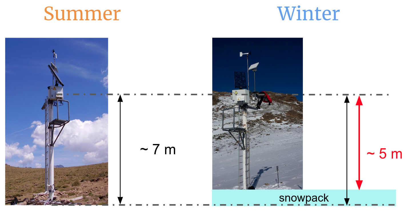
Figure 1A Nivose station in summer and winter (here the Sponde Nivose station, Albertacce, Corsica). The temperature sensor (top dotted line) is located about 7 m above the bare ground (bottom dotted line). Assuming for this example that the average height of the snowpack is 2 m, the sensor is located about 5 m above the surface (red arrow) in winter.
Another fundamental use of screen-level temperature observations in operational NWP is their assimilation to improve the representation of the atmospheric state prior to forecasting its evolution over the upcoming hours and sometimes days (Brousseau et al., 2016; Demortier et al., 2024; Guillet, 2019; Gustafsson et al., 2018). Indeed, a good initial state is mandatory for accurate weather forecasting. As a matter of fact, the progress of NWP systems in recent decades has been very driven by the increase in data assimilation, especially relying on satellite data (e.g., Fischer et al., 2018). In Arome-France, screen-level temperature observations are used in two different assimilation systems (Fig. 3 and Sect. 2.2), respectively majorly affecting the surface (Marimbordes et al., 2024) and the atmosphere (Brousseau et al., 2016). However, the height-above-ground specificities of high-altitude stations are not accounted for in either assimilation system, and data from the Nivose stations are assimilated as if they were measured at 2 m. As an illustration, Fig. 3 in Marimbordes et al. (2024) shows a map of so-called “2 m temperature observations stations that are assimilated” in the surface assimilation. This map includes high-altitude (> 3000 m a.s.l.) stations from the Météo-France “Nivose” observation network that actually measure air temperature at roughly 7 m above snow-free ground. Therefore, a second part of the present study will be dedicated to the impact of the height mismatch between observations and the model in terms of assimilation. More precisely, we examine the way Arome assimilates mountain near-surface temperature observations as a possible cause for biases observed in Arome.
Finally, in situ observations from mountain regions are inherently heterogeneous when it comes to their topographic context. The complex topography can result in a significant discrepancy between the model relief at the nearest point of a station and the actual altitude of the station. Most stations are furthermore in valleys or mid-altitude areas, where accessibility and maintenance are made easier. This results in a spatially and altitudinally inhomogeneous distribution of observations (e.g., Vernay et al., 2022; Thornton et al., 2022). While model evaluations in complex terrain regions quite often discriminate results either into altitude bands (e.g., Vionnet et al., 2016; Monteiro et al., 2022) or classes derived from landforms (ridges, crests, valleys, plains, e.g., Winstral et al., 2017), such distinctions are not made in assimilation. The structure functions that propagate the analysis increment spatially do sometimes account for the topographic and landform heterogeneities (e.g., Deng and Stull, 2005), but this is not the case in Arome for the 3DVar atmospheric assimilation system. In the last part of the Results section, we also therefore scrutinize how these spatial heterogeneities of the observation network with respect to topography affect the quality and efficiency of screen-level temperature assimilation into the Arome NWP system.
In a nutshell, the present study intends to shed light on some challenges associated with the use of the near-surface air temperature observations in mountain terrain for numerical weather forecasting by addressing a series of research questions.
-
Taking the example of the Arome-France NWP system that operationally runs over a large alpine region, we will first address the question of the impact of varied sensor height above the surface on the assessment of model performances. One of the underlining questions is whether observations acquired at 2 m to about 5 m above the snow surface can be used without specific treatment to evaluate model performances or whether they should be considered separately as revelatory of different model behaviors. Through this analysis, we intend to provide guidelines for the use of temperature measurements for model evaluation in mountain regions.
-
In a second subsection of the Results section, we will evaluate the effect of this height heterogeneity on the way the model is corrected by assimilation. This subsection will answer the question of whether the height of the observation above the surface matters for assimilation or whether it is not necessary to discriminate between temperatures from 2 to 5 m above the surface for the assimilation. In particular, we will examine the assimilation of mountain near-surface temperatures as a possible cause for the cold bias of Arome.
-
Finally, another question poorly addressed in existing literature is how the relief mismatch between observation stations and model grid cells, as well as valley vs. mountain heterogeneities in terms of observational density, affects the efficiency of data assimilation. We will address this question in the Results section of this study through the use of dedicated assimilation experiments.
The plan of our paper addresses these items sequentially, after a section dedicated to materials, methods, and study area. To the best of our knowledge these questions have not thoroughly been addressed in midlatitude mountain regions of the world. We focus on winter conditions as the period when the model biases are the strongest. We also take the opportunity to propose in the Discussion section perspectives to circumvent the problems highlighted for the benefit of weather forecasting in complex terrain.
The main abbreviations or acronyms used in this section and throughout the paper are summarized in Table A1.
2.1 Study area and in situ data
2.1.1 Domain and time period
The study focuses on the alpine massifs (Fig. 2: map on the right) as the mountain range having the highest number of meteorological observations and the most complex relief in France. In winter, the biases of the Arome model in terms of 2 m temperature (T2m) are particularly important over this area (Paci et al., 2016; Vionnet et al., 2016; Dombrowski-Etchevers et al., 2017). The study period ranges from 2020 to 2023 and therefore covers almost four winters (December, January, and February): the winters 2019–2020 (with December missing), 2020–2021, 2021–2022, and 2022–2023.
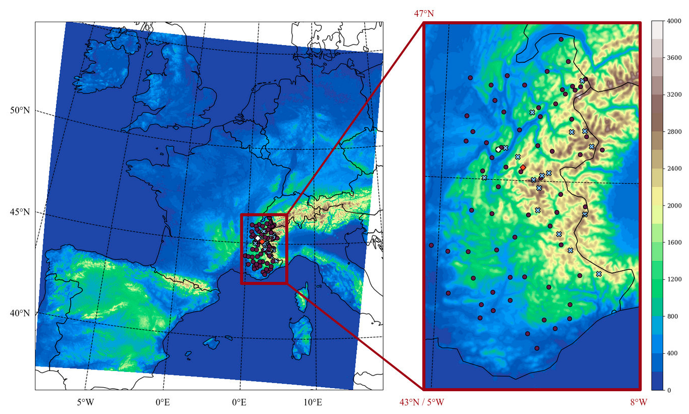
Figure 2Relief of the model over the Arome-France domain with a zoom on the study domain and the measurement stations. The stations of the Météo-France standard network are shown in purple and those of the Météo-France Nivose network in blue, except for Col de Porte-Nivose, which is in white due to co-location with a well-instrumented site, and the instrumented station at Col du Lac Blanc in red.
2.1.2 In situ data
This study makes use of the Météo-France operational observational network and of well-instrumented research sites described hereafter (Fig. 2). In particular, due to the mountain and assimilation focuses of the study, the operational stations used are those located in the Alps and its foothills (Pre-Alps) and taken into account by the altitude 3DVar assimilation system of Arome.
Well-instrumented mountain sites
-
The mid-altitude Col de Porte site (CDP, 1325 m). Col de Porte (here after CDP) is an observation and research site located at 1325 m in the western side of the French Alps (white dot in the Fig. 2). Several variables are measured there (Morin et al., 2012; Lejeune et al., 2019), including surface and near-surface air temperatures, the latter being always measured approximately between 1.5 and 2 m above the surface: during the snow season, the height of this temperature sensor is adjusted manually above snow surface at weekly intervals so as to be maintained at a constant height over the snowpack. We will consider this observation to be the temperature at 2 m in this paper. Besides, this instrumental site also includes a Nivose station (see later in this section for a more complete description of such stations), measuring the temperature at approximately 5 m above the snow surface in winter.
-
The high-altitude Col du Lac Blanc site (CBL, 2720 m). Col du Lac Blanc (here after CLB) is an experimental site located at 2720 m in a slightly more inner location within the French Alps (red dot in the Fig. 2). The site was originally dedicated to the study of wind-induced snow transport (Guyomarc'h et al., 2019; Vionnet et al., 2013; Naaim-Bouvet and Truche, 2013). It features various instruments including incoming and outgoing longwave and shortwave radiation, as well as a mast equipped with temperature and humidity sensors located at 2, 3.2, 5, and 7 m above the snow-free ground. Snow height is also measured directly at the mast so that the height of each sensor over the snow surface can be known during the snow season. This enables the temperature at 2 m above the snow surface to be retrieved by linear interpolation between the two sensors closest to that height. We also make use of the temperature measured at approximately 5 m above the snow surface in winter at a station configured like a Nivose but used only for research purposes. This station features a temperature sensor at 7 above snow-free ground (Lac Automatic Weather station, Guyomarc'h et al., 2019). Snow is always present during the study period in winter. Assuming that its emissivity is 0.98 (Dozier and Warren, 1982), the surface temperature can be calculated from the outgoing longwave radiation by inverting the Stefan–Boltzmann law.
Météo-France surface observation network
-
Standard stations. By “standard stations” we designate the stations from the RADOME network consisting of automatic stations providing hourly surface data to Météo-France, (shown in purple in the Fig. 2) with exceptions for the Nivose, considered separately (see below).
-
Nivose stations. Within the RADOME network, some stations are specifically designed for high-altitude areas. They are called Nivose stations and are mainly located above 2000 m in the main massifs of metropolitan France (blue dots in Figs. 2 and 1). They measure wind, temperature, and humidity at a height much higher than 2 m above bare ground in order to provide data despite a deep snowpack in winter. Generally, the temperature sensors are placed at about 7 m above the bare ground, with ±0.5 m variability depending on site configuration.
2.2 The Arome numerical weather prediction system and its assimilation
The limited-area NWP model Arome (Application de la Recherche Opérationnelle à Méso-Échelle) has been operational since December 2008 and runs over the domain named “France”, illustrated in Fig. 2. It is coupled to the French global model Arpege (Action de Recherche Petite Échelle Grande Échelle), which has a variable spectral mesh (Courtier and Geleyn, 1988) and improved resolution over Europe. Initially with a horizontal resolution of 2.5 km (Seity et al., 2011), Arome has been producing forecasts on a 1.3 km grid since April 2015 (Brousseau et al., 2016). Its physics scheme is the same as Meso-NH (Mesoscale NonHydrostatic Model) (Lafore et al., 1998; Lac et al., 2018). Thus, it is a non-hydrostatic model; i.e., it “explicitly solves the system of compressible Euler equations without neglecting the vertical acceleration in the continuity equation, which allows a better representation of vertical motions or orography” (Arnould et al., 2021). Arome uses the dynamics of the Aladin model (Adaptation Dynamique Développement International; Bubnová et al., 1995). Although the first version of Arome had 60 vertical levels with the first level at 10 m above the surface, the version now used operationally has 90 vertical levels, the first of which is between 4.5 and 5.5 m in the model, depending on weather conditions, i.e., approximately 5 m. As a research option, a version of this model is available with 500 m horizontal resolution and/or 120 or 156 vertical levels (with the lowest level at 2.5 m approximately).
For the surface scheme, Arome is coupled to SURFEX (Surface EXternalised; Masson et al., 2013) (orange boxes in Fig. 3), with, for vegetation, the Isba (Interaction Soil–Biosphere–Atmosphere; Noilhan and Planton, 1989) scheme and, for snow, the D95 single-layer scheme (Douville et al., 1995).
To ensure that the model is as close as possible to the real state of the atmosphere, it is regularly corrected using observations. This process is called data assimilation and is described for near-surface temperatures in Fig. 3. For simplicity in the following, we will refer to near-surface air temperature as T2m, despite the fact that it is conventionally measured between 1.25 and 2 m above the surface following the WMO standards and between 1.5 and 2 m according to the French Meteorological Service standards. When referring to modeled values for near-surface temperatures, we will also use the term T2m (often with the suffix “_mod”). In that case, T2m refers to a temperature diagnostic produced by the model for a 2 m height above the surface.
In Arome, the assimilation takes place both in the atmosphere and at the surface (the blue and green boxes in Fig. 3, respectively), but without interaction. In addition, the assimilation methods differ. Furthermore, the presence of fields dating from before the use of SURFEX is necessary for the assimilation to run smoothly, whether for the atmosphere or the surface (grayed-out box in Fig. 3).
For convenience, in the diagram and in the rest of the article, T5m_mod will refer to the temperature at the first level of the model, which is approximately at 5 m above the surface. The surface temperature (Ts_mod) corresponds to the surface temperature of the ground for Arome. If this ground is snow-covered, then it becomes the surface temperature of the snow cover (Giard and Bazile, 2000). T5m_mod and Ts_mod are prognostic variables. These two temperatures are used to compute T2m_mod according to Geleyn (1988)'s diagnostic.
2.2.1 The 3DVar altitude assimilation
The assimilation of atmospheric variables in Arome is based on the 3DVar (three-dimensional variational system) (Fig. 3 b), with an hourly data assimilation cycle (Brousseau et al., 2016; Gustafsson et al., 2018). The aim is to provide the best possible estimate of the state of the atmosphere at a given time. To achieve this, the atmospheric fields predicted by the model are used as the “background state” of the atmosphere, also commonly called a “guess”, which is then combined with observations to minimize the difference between both (Guillet, 2019). In the case of 3DVar, the background corresponds to a 1 h Arome forecast (T2m (diag)(P1) in Fig. 3a) calculated before each analysis on the basis of the previous analysis (T2m (diag)(P0) in Fig. 3c). Before their assimilation, all observations, whether satellite or surface data, are first subjected to a quality control known as “screening”. This step eliminates observations that are considered doubtful because they come from a non-qualified source or are too far away from the background. However, if this background is biased, the screening can also reject observations that come from accurate measurements and contain valuable information for the assimilation.
After screening, the 3DVar combines the observations with the background (Fig. 3b) to produce the new analysis by minimizing the cost function J (Demortier et al., 2024):
where xb corresponds to the background state, yo to the observation vector, and ℋ to the (nonlinear) observation operator, which allows different types of information to be compared; R and B are the observation and background error covariance matrices. The matrix B contains background error covariances in the spectral space. This dependence on the spatial neighborhood depends on the correlation lengths of the errors, which in Arome are spatially uniform and do not take into account relief. Furthermore, this B matrix is constant in time. Background departures are calculated for the surface observations and for the upper-air observations. Then, J is minimized using these background departures. However, the increment of surface observations is calculated at 2 m but is not carried upstream to the height of the first level of the model before being used.
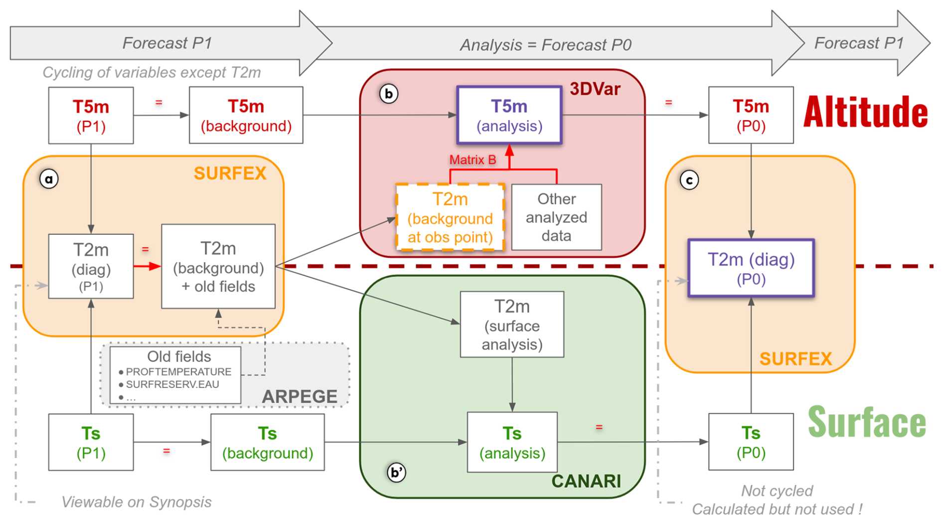
Figure 3Workflow of the near-surface air temperature assimilation in Arome, featuring the altitude assimilation system (above the red dotted line) and surface assimilation system (below the red dotted line). The term “diag” refers to a diagnostic variable, P1 to the first term of a forecast, and P0 to the initial state prior to a forecast and after the analysis step. The color boxes specifically highlight the altitude 3DVar analysis scheme, the surface Canari analysis scheme, and the diagnostics performed for T2m in the surface scheme, SURFEX.
2.2.2 The Canari OI surface assimilation
For the surface, the analysis is computed by the Canari system (Code d'Analyse Nécessaire à Arpege pour ses Rejets et son Initialisation) (green box of Fig. 3) using the optimal interpolation (OI) method described by Taillefer (2009):
where xa corresponds to the analyzed state of the model.
Firstly, as with altitude assimilation, a quality control process eliminates observations considered to be unrealistic. For this stage, the same equation is used, but the control parameters do not have the same value. It therefore sometimes happens that certain observations are rejected in the altitude assimilation and kept in the surface assimilation. OI is an assimilation method particularly suited in the context of rather scarce data, when a limited number of observations are used to determine the analyzed state (e.g., Durand et al., 1993). So, unlike 3DVar, the observations deemed strategic are interpolated at the grid point by a so-called structure function, which models the background error covariances, i.e., B, a static and univariate matrix that does not account for correlations between, e.g., T2m and humidity at 2 m, another analyzed observation. In our study as in operational Arome, the Mescan (contraction of MESoscale analysis and Canari) option (Mahfouf et al., 2007; Van Hyfte, 2021) activates this function which uses a correlation length of 100 km varying according to the difference in altitude between the grid point and the observations (Marimbordes et al., 2024). Thus, using 2D optimal interpolation and the Mescan structure function, the analyzed temperature and relative humidity fields at 2 m are obtained (Ts (analysis) in Fig. 3b'). The T2m and Hu2m increments calculated in the 2D canary step are then used to compute the surface analysis, i.e., the surface temperature, average soil temperature, surface soil humidity, and average soil humidity (Giard and Bazile, 2000) at each point using 1D OI. The analyzed surface temperature is involved in the estimation of the analyzed temperature at 2 m via a diagnostic (Fig. 3c).
2.3 Scores
In the present study we use scores to quantify the agreement of model results with in situ observations. In these scores, and to quantify the impact of ill-suited relief, the stations which present more than 150 m altitude difference with their model grid point are by default not discarded. The following scores will be used:
-
an hourly mean bias defined as Bias , where N is the total number of stations and days during the studied period.
-
a root mean square error or RMSE which calculates an average magnitude of differences between predicted and observed values: RMSE , where N is the total number of stations and time steps during the studied period.
As the RMSE alone does not show if a simulation is too warm or too cold compared to reality, the RMSE will be studied in conjunction with the bias. These calculations will be done over the whole study period.
In addition, the scores will be also computed by altitude bands (Table 2), i.e., separately for areas below 1100 m, between 1100 and 2000 m, and above 2000 m. This enables us to distinguish between valley, mid-altitude, and high-altitude areas, respectively, as atmospheric conditions vary according to altitude (e.g., Chow et al., 2013; Whiteman, 2000) and Arome exhibits different biases across altitudes (Vionnet et al., 2016; Dombrowski-Etchevers et al., 2017; Monteiro et al., 2022).
2.4 Assimilation experiments
2.4.1 Experiments
Targeted numerical experiments are carried out in order to analyze the effect, on the assimilation, of geographical or measurement inhomogeneities specific to mountain regions. These experiments consist of modifying the observations assimilated or the conditions in which they are assimilated. These numerical simulations are compared to a reference, which is the operational Arome forecast (Arome-OPER) described in more detail hereafter. This reference is also the one evaluated in the present study when scores and biases are mentioned without further specification.
-
Arome-OPER. The objective of this reference (OPER for operational version of Arome described in Sect. 2.2) is to identify and quantify the Ts, T2m, and T5m biases, be they due to the assimilation or to the modeling of processes in mountainous terrain. The forecasts are extracted from the daily 00:00 h run of the study period, the background (orange-bordered box entitled “T2m (background at obs point)” in Fig. 3) and analysis (blue-bordered box entitled “T2m (background at obs point)” in Fig. 3) of T2m are retrieved from the 3DVar at each hour, and the analyzed temperatures (purple-bordered boxes entitled “T2m (diag)(P0)” and “Δ T5m (analysis)” of Fig. 3) come from the hourly analysis file.
-
NO_VALLEY. In this numerical assimilation experiment, observations of T2m and relative humidity at 2 m (RHU2m) below 1100 m a.s.l. are excluded before entering the 3DVar. The goal is to quantify the impact of valley stations on assimilation in higher-altitude areas. The value of the 1100 m threshold is set so that this experiment does not take into account the data supplied by stations located in the highest valleys the French Alps, such as the Chamonix-Mont Blanc valley with an automatic station at 1042 m a.s.l. The results of this experiment will be studied over the winter of 2022–2023.
-
NO_NIGHT. The diurnal cycle influences the T2m bias, which peaks at night in mountainous areas (Vionnet et al., 2016; Dombrowski-Etchevers et al., 2017). The Austrian version of Arome, operated by Geosphere Austria, does not use assimilation overnight. This raises the question of the impact of nighttime data assimilation on the Arome-France. To quantify this, in this “NO_NIGHT” experiment, T2m and RHU2m are not assimilated at night, i.e., when the solar angle is less than 10°. The impact of NO_NIGHT is evaluated for the winter of 2022–2023.
-
150M. In mountains, the difference between the actual altitude and the model altitude can vary significantly. For example, Mont Blanc is at 4318 m for Arome 1.3 km compared with 4809 m in reality. Currently, no criteria on altitude mismatch between the model grid point and observation station are applied to T2m assimilation in Arome. However, Quéno et al. (2016), Vionnet et al. (2016), and Dombrowski-Etchevers et al. (2017) considered the observations to be relevant to evaluate model performances and calculate scores as long as this vertical distance was less than or equal to 150 m. This criterion was chosen as it corresponds to a 1 °C difference when considering a standard atmospheric gradient of 6.5 °C per vertical kilometer. In this “150M” experiment, we apply this 150 m threshold and do not assimilate station data when their altitude differs more than 150 m from their grid point altitude in the Arome model. As a result, 13 stations are not assimilated. This numerical simulation is analyzed for the winter of 2022–2023.
2.4.2 Analysis of the experiments
In the Sect. 3.3, the abovementioned assimilation experiments will be analyzed to quantify the effect of varying observational network characteristics onto the assimilation result (i.e., the analysis). These characteristics include the exclusion of valley and flatland stations, of all surface stations at night, and of stations for which the altitude difference with respect to the model grid cell exceeds 150 m. To highlight the effect of these variations in observational networks, we make use of the analysis increment Δ, whereby
with xa the analyzed model state and xb the background model state prior to assimilation.
At observation stations, an ideal analysis increment would enable the analysis to fully coincide with the observation. We therefore define the ideal analysis increment at stations as
where xobs denotes the observation.
The NO_NIGHT experiment, disabling the assimilation of surface observations at night, enables us to highlight the effect of the altitude observations only for the nighttime period. We hence call for the nighttime period
For the nighttime period, we can hence define a virtual analysis increment coming from the analysis of surface observation only, , by considering the following relationship between the analysis increment of the Arome-OPER experiment (ΔOPER) and the ones that respectively result from the assimilation of altitude (Δobs_altitude) and surface observations () only:
In practice, this virtual analysis increment for surface observations only likely differs from the one that would have been calculated by disabling the altitude analysis due to compounding effects between altitude and surface observations. In the decomposition proposed in relation (6), these compounding effects are integrated in the surface observation analysis increment , hence distinguished as a virtual increment analysis, and we do not have the possibility to quantify them.
Similarly, the analysis increment of Arome-OPER can also be decomposed into the virtual contribution from the flatland and valleys and what comes from the upper-air and mountain stations only included in the NO_VALLEY experiment. According to this decomposition,
and also
where relation (7) enables us to retrieve , while relation (8) enables us to retrieve the contribution from mountain stations only among surface observations, .
Another possible decomposition of ΔOPER reads
where () is the virtual analysis increment for surface stations with more (less) than 150 m altitude departure with respect to model relief, while Δ150M refers to the 150M experiment.
In these latter relations, similarly to the increment, the virtual increments, denoted by a v exponent, are not directly calculated from an experiment but diagnosed from a complementary experiment and therefore include compounding effects that cannot be isolated.
These different increments will be used in the Results and Discussion sections to analyze the effects of heterogeneities in the observational network in Alpine terrain on the assimilation in Arome.
3.1 Impacts of heterogeneous sensor height on model evaluation
In this section, we closely examine the impact of differences in height between standard temperature measurements (at about 2 m above surface) and measurements from high-altitude networks (at rather 5 m above the surface during the snow season) in terms of model evaluation over the winter season. In the Introduction we illustrated how temperature actually measured at 5 m above the surface in winter in high-mountain regions is commonly considered to be at 2 m when evaluating atmospheric models, an assumption that we will refer to as “error in measurement height”. We will first examine the comparability between temperatures observed at 2 and 5 m above the surface for well-instrumented sites in winter. Then, we will scrutinize how both temperatures compare in the Arome model world and with respect to observations. Finally, we will derive the impact of the commonly made error in measurement height on the scores obtained when comparing the Arome model to observations.
3.1.1 Comparison between observed T2m and T5m at the well-instrumented sites
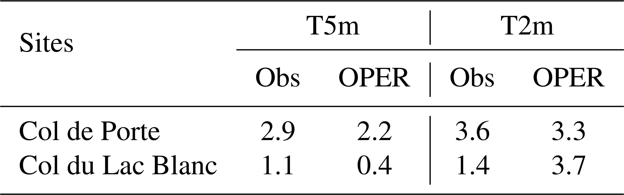
Figure 4 features the diurnal cycles of temperatures retrieved for the surface (Ts) and at 2 and 5 m at the CDP and CLB sites. The same diurnal cycles obtained in the Arome-OPER forecasts are also shown and will be analyzed later (note that a complementary figure, Fig. B1 in the Appendix, enables an easier comparison between all temperatures at each site at the expense of general readability). We observed a mean difference between observed T2m and T5m of 0.3 °C at CDP (0.4 °C at CLB). Such a difference is not significant at CLB with respect to the measurement uncertainty, which is expertly estimated to be within ±0.5 °C based on the numerous co-located temperature measurements and the use of temperature shelters of different designs (Guyomarc'h et al., 2019). Despite a higher accuracy for the T2m observation at CDP, estimated by Morin et al. (2012) to within 0.1 °C, the T5m Nivose measurement from the CDP probably has a lower accuracy, likely similar to the one estimated at CLB. Although their mean values are not significantly different, the daily cycles of T5m and T2m observations significantly differ, with a maximum difference of 0.6 °C at 09:00 UTC at CDP (and 0.5 °C at 05:00 UTC at CLB; Fig. 4a and b). In addition, the root mean square difference between observed T5m and T2m over winter is also significant with a value of 0.6 °C at both sites. We finally find that differences between 2 and 5 m measurements are also significant in terms of thermal amplitudes at the CDP (Table 1, Obs columns). We note that the difference between T2m and Ts is significantly more marked than the one between T2m and T5m in the observations, with an average difference of 4.8 °C at the CDP and 3.2 °C at the CLB; the maximum difference amounts to 6.5 °C at 10:00 UTC and 4.2 °C at 07:00 UTC at CDP and CLB, respectively.
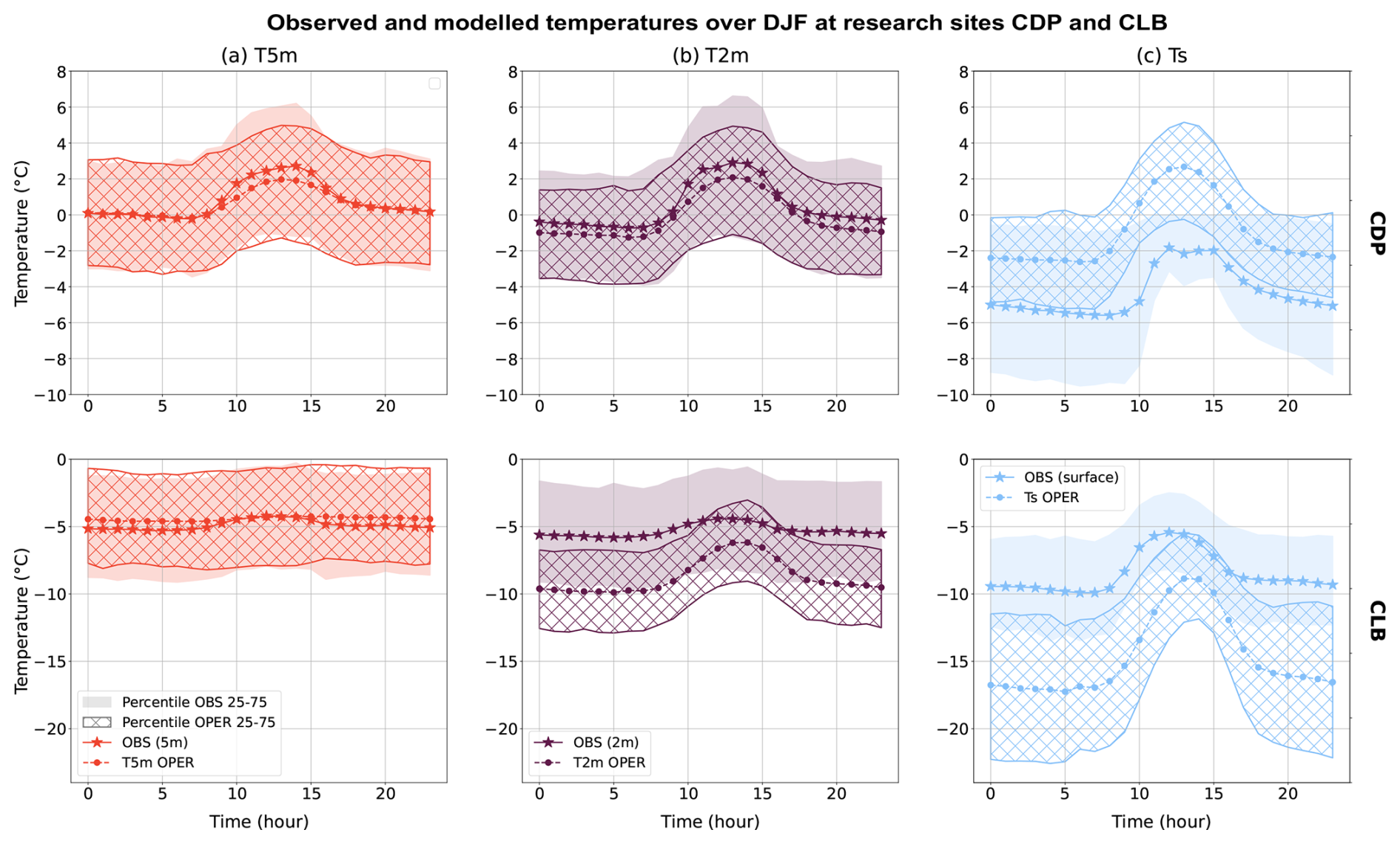
Figure 4Diurnal cycle of the 5 m (a, red), 2 m (b, violet), and surface (c, blue) observed (OBS) and modeled (OPER) temperatures averaged over the winters of the study period at the CDP and CLB research sites. The shaded (hatched) areas represent the observed (modeled) variability via the 25 %–75 % percentile range.
Table 1Thermal amplitude of temperatures T5m and T2m observed and modeled by Arome-OPER at CDP and CLB over the winters (DJF) between 1 January 2020 and 28 February 2022.
Further analyses show that the differences between observed T2m and T5m can be much higher than the mean values during specific situations, especially during stable conditions when stratified cold air covers the Alps. The dates 19 and 20 December 2021 typically illustrate this kind of situation (Fig. 5a).
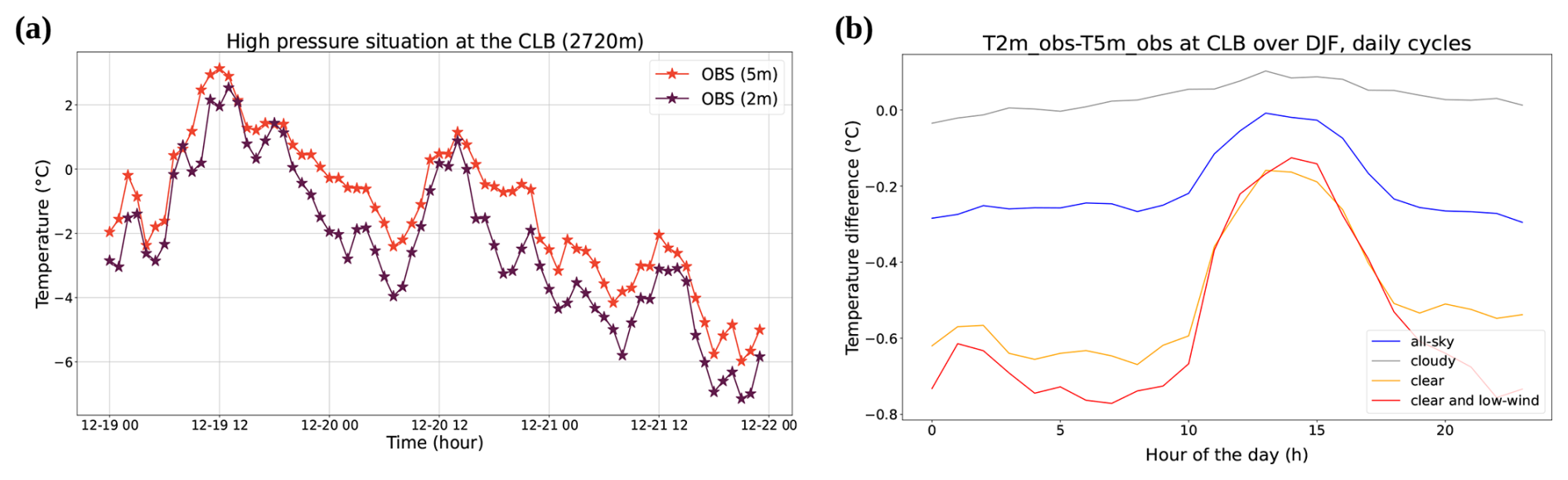
Figure 5(a) Temporal evolution of temperatures observed at 2 m (purple) and 5 m (red) from 19 December 2021 at midnight to 21 December 2021 at 11:00 p.m. at the Col du Lac Blanc. (b) Diurnal cycles of differences between T2m_obs and T5m_obs at CLB over one winter season. Clear-sky (cloudy) situations refer to days with an average effective atmospheric emissivity lower than 0.7 (higher than 0.9), which correspond roughly to the lower and upper quartile of the daily effectivity distribution at the CLB (Gouttevin et al., 2023). Low wind conditions are considered when wind is lower than 4 m s−1.
During this period, the Alpine massif is under the influence of an anticyclone centered on northwestern Europe and reaching up to 1040 hPa. Close to the surface, the winds are weak and from the east. Despite cloudy weather on the plains, the Alps are, on the other hand, under clear skies. During this period, the sun sets around 05:00 UTC for the summits of Grandes Rousses, the massif where the CLB is located. In these stable winter conditions, the nocturnal radiation and the snow then present on the ground induce a very strong inversion in the low atmosphere (Pepin and Kidd, 2006). This generates a marked gradient between T5m and T2m at CLB of up to 2.5 °C at 07:00 UTC on 20 December. A similar behavior was also highlighted by Gouttevin et al. (2023) for Arome-OPER at the CLB and at another high-altitude site, with a strong stratification in air temperatures in the lowermost boundary layer during clear-sky, low winds conditions, as supported by Fig. 5b. While cloudy sky situations feature a very homogeneous, non-stratified lower boundary layer, clear-sky days (especially with low wind) feature a strong temperature gradient between the surface and the air higher up so that the difference between T2m and T5m is on average distinctively lower than −0.5 °C at night and even lower than 0.65 °C in low wind conditions.
We conclude from this section that considering T2m and T5m as fully equal temperatures is an invalid approximation at both our mid- and high-altitude sites: the difference between T2m and T5m is weak and within the measurement uncertainty on average over winter but is not so during certain weather situations. Indeed, in anticyclonic weather, particularly at night with clear skies and low winds, this difference can be greater than 2 °C and therefore very significant. Furthermore, differences exist in the diurnal cycles and amplitudes. Consequently, when using the observations at 5 m of the Nivose stations as if they were at 2 m, an error is introduced in the calculation of the scores, especially of error scores like the RMSE typically used to qualify operational forecasts (Vionnet et al., 2016; Dombrowski-Etchevers et al., 2017) and their improvements.
3.1.2 Comparison between forecasted T2m and T5m at the well-instrumented sites
Figure 4a and b also show the diurnal cycles of T5m_mod and T2m_mod simulated by Arome-OPER at CDP and CLB. The difference between these cycles is significant, with a mean difference of 0.7 °C at CDP (and 4.3 °C at CLB) and a maximum difference of 1.1 °C at 02:00 UTC at CDP (5.3 °C at 05:00 UTC at CLB). The average difference between the modeled temperatures is therefore much larger than between the observed temperatures (of 133 % at CDP and 975 % at CLB). Moreover, the gradient between the T5m_mod and T2m_mod is significantly stronger at the CLB than at the CDP.
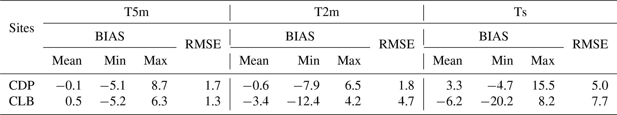
If we compare the model to observations at 5 and 2 m over the three winters of our study period (Fig. 4), we note that Arome slightly overestimates the T5m at CLB with an average bias of 0.5 °C (Table 2) and underestimates it at CDP during daytime, with for the latter site a maximum bias of −0.8 °C at 10:00 UTC (Fig. 4a, Table 2). Besides, the RMSE of the model at both sites has a similar value, higher than the bias. Hence, although Arome is on average weakly biased at 5 m, it suffers from biases in certain weather conditions. As a further illustration, the maximum negative error of T5m_mod over the three winters falls to −5.1 °C at CDP (−5.2 °C at CLB), while the maximum positive error reaches 8.7 °C at CDP (6.3 °C at CLB, Table 2). On the other hand, the model is too cold at 2 m at both sites, with an average bias of −0.6 °C at CDP (−3.4 °C at CLB, Table 2). As with T5m_mod, the mean value of the bias at CDP does not reflect the dispersion of T2m_mod, for which the bias ranges from −7.9 to 6.5 °C (Table 2). The bias and RMSE are stronger at 2 m than at 5 m, particularly at the high-altitude site. Arome hence represents temperature with a better accuracy at its first level than at 2 m.
Table 2Scores of Arome-OPER at CDP and CLB over the winters (DJF) between 1 January 2020 and 28 February 2022.
We conclude from these results that the T5m_mod and the T2m_mod cannot be considered as equivalent and approximated by each other in Arome. As a result, the height of the sensor should be taken into account when the model is compared to observations.
3.1.3 Assessment of forecasted T2m and T5m across the Alps
We confirm the results obtained at the two research sites in the previous subsections, with an analysis of the differences between the Arome-OPER (forecast) T2m and T5m across the study area: Fig. 6a illustrates how the mean winter T2m_mod minus T5m_mod difference evolves as a function of altitude over the French Alps during winter 2021–2022. While the median of this mean difference is on the order of 0 to −2 °C for altitudes lower than 1700 m a.s.l., the mean temperature difference drastically drops to median values below −4 °C for altitudes above 2000 m with extreme mean winter differences close to −8 °C. Above 2400 m a.s.l., 95 % of the mean differences between T2m_mod and T5m_mod are below −2 °C. Furthermore, the biases in Arome-OPER assessed at the CLB and CDP sites are partly representative of the biases generally found across the French Alps, as shown in Fig. 6b: this figure compiles the mean winter biases of Arome in terms of T2m and T5m, as calculated at all standard and Nivose stations, and also including the research sites. A warm bias affects T2m_mod in mid-altitude mountains up to around 1600 m, with the observations at CDP deviating from this pattern with a slightly negative T2m bias.
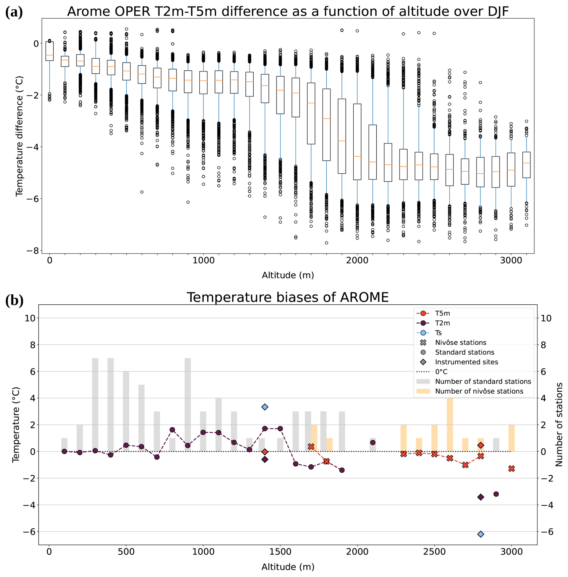
Figure 6(a) Arome-OPER mean temperature differences between 2 and 5 m as a function of altitude for each model grid point over the study area for winter 2021–2022. The orange line denotes the median, box plots mark the 25th–75th percentiles, blue whiskers mark the 5th–95th percentiles, and dots mark the values outside this range. (b) Arome-OPER temperature biases at 5 m (red dashed line) and 2 m (violet dashed line) at Nivose stations (crosses), standard stations (dots), and instrumented sites (diamonds) over the winters of the 2020–2022 period. Bias is calculated by grouping stations by 100 m altitude bands and by station type. The altitude range shown in the figure, e.g., 600 m, corresponds to stations with an altitude between 500 and 600 m. The number of stations used to calculate the biases is indicated by bars with the Nivose stations in orange and the standard stations in gray. The Col de Porte station is counted here as an instrumented site, not as a Nivose station.
The thermal amplitude of the diurnal cycles for the T2m and T5m observed and forecast temperatures is reported in Table 1 for both CDP and CLB. At CDP, simulated amplitudes are relatively close to observations, with a slight underestimation for T5m and T2m. At CLB, the amplitude for T5m is underestimated. On the other hand, it is overestimated for T2m. Arome attenuates the diurnal cycle too much at the first level of the atmosphere and accentuates it too much close to the surface.
3.1.4 Reviewing scores and revisiting model biases
As T2m and T5m should not be considered equivalent, the T2m scores of Vionnet et al. (2016) and Dombrowski-Etchevers et al. (2017) at high Alpine or Pyrenean stations should therefore be put into perspective as temperature observations at 2 and 5 m above the snow surface were used without distinction. According to Gouttevin et al. (2023), based on detailed evaluations at two high-altitude sites, the temperature scores at about 10 m show that the Arome model is only slightly biased at this level. We therefore propose revisiting the general scores of Arome over the Alps (as estimated by Vionnet et al., 2016, and Dombrowski-Etchevers et al., 2017), making a clear distinction between the first model level at about 5 m above the surface and 2 m. In Fig. 7 and Table 3, bias and STDE scores were therefore calculated one the one hand for stations above 2500 m altitude (Nivose stations only) by comparing the T2m diagnosed by Arome and the temperature observed at the Nivose stations between November 2022 and May 2023, according to the method used by Vionnet et al. (2016). As these scores/biases are calculated assuming that the stations measure at 2 m above the surface, they are not true biases or RMSE at 2 m, and we hence call them “pseudo-biases” in the following. On the other hand, the same scores were obtained using the T5m_mod forecasted by Arome (leading to true T5m biases and scores). The stations with an altitude difference of more than 150 m from their model grid point have been removed from the calculation of these scores. Indeed, although the standard vertical temperature gradient of −0.65 °C/100 m is often applied to account for this difference between model relief and real relief, this is not the correct solution (Sheridan et al., 2018). In the mountains, the altimetric temperature gradient is rarely equal to −0.65 °C/100 m: it can be null in the case of isothermal conditions with snow precipitation, positive in the case of inversions, or strongly negative. Table 3 compares the old and the new revisited scores.
Vionnet et al. (2016)Table 3Bias and STDE for Nivose stations according to the Vionnet et al. (2016) method (comparison with T2m_mod) and new method (comparison with T5m_mod).
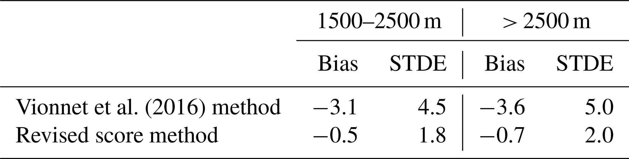
The cold bias decreases by 2°, while the STDE decreases by 1° only by comparing temperatures at an equivalent height above ground level. It therefore has a significant impact on scores to evaluate models in relation to comparable observations and to bear in mind their representativeness. Taking sensor height into account has a greater impact on scores than applying an altitude correction that is potentially false. The monthly temperature bias at high-altitude Nivose stations calculated for 4 months (January, April, August, and November) by Dombrowski-Etchevers et al. (2017) (same method as Vionnet et al., 2016) has been recalculated for the period 2022–2023, on the one hand using T2m_diag (as initially) (see Fig. 7a) and on the other using T5m_mod (see Fig. 7b). Monthly biases are much lower when comparing with T5m_mod than with T2m_diag, as expected. It is no longer the months with snow on the ground that are the most biased, but the months with the most solar radiation. The nocturnal bias is virtually null (slightly positive), while the diurnal bias is negative. The graph showing T5m, T2m, and Ts predicted by the model versus observations confirms what was highlighted at CLB and CLP in Fig. 4. In addition, the month of April is undoubtedly the most biased due to the excessive presence of snow on the ground in the model (a bias mentioned by Monteiro et al., 2022), which further limits the heating of the atmosphere by the surface.
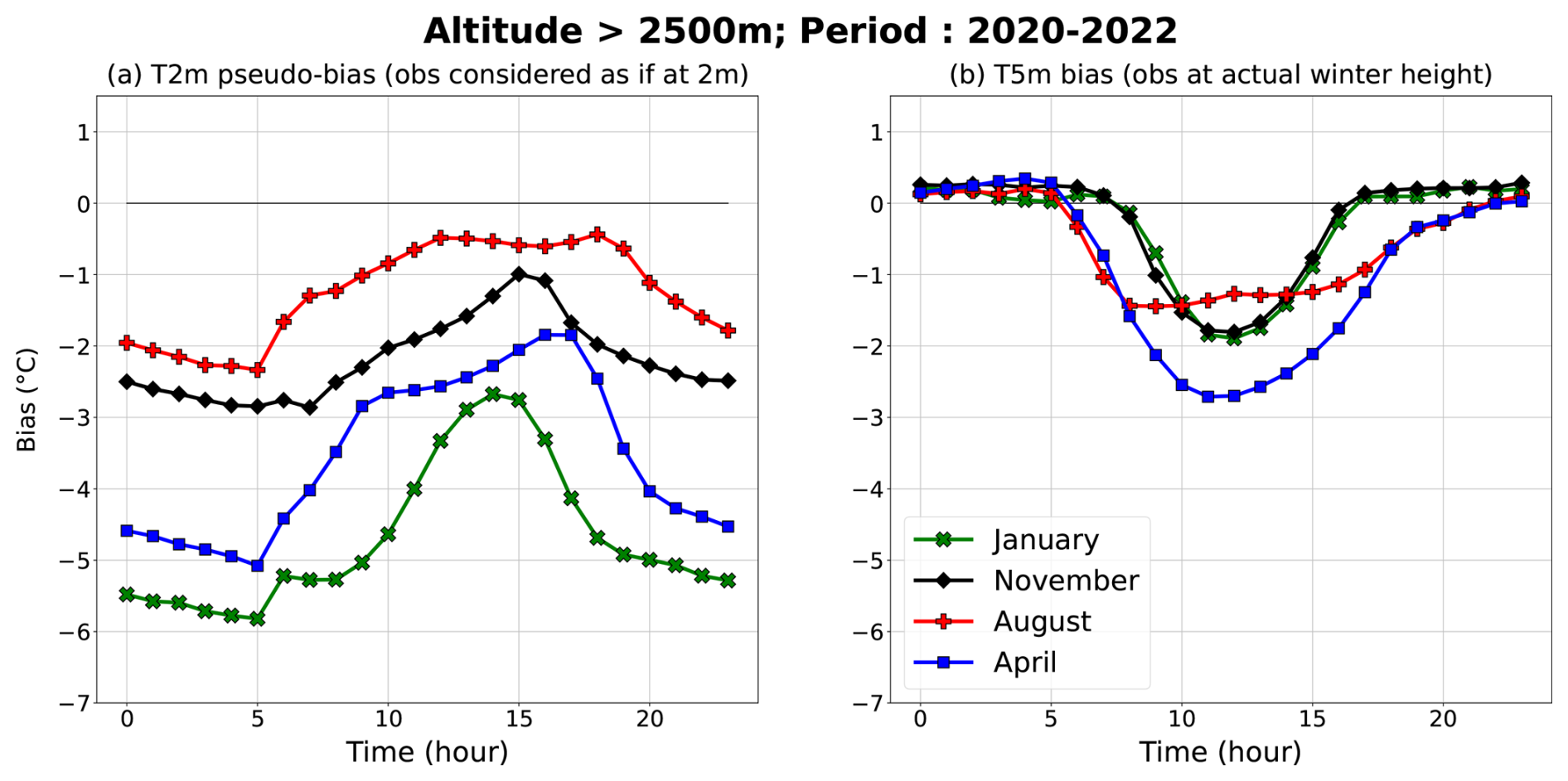
Figure 7(a) Diurnal cycle of the T2m bias calculated according to Vionnet et al. (2016), i.e., without taking into account the sensor height, and (b) true T5m bias, estimated based on T5m_mod. Only T5m_obs values from Nivose stations for the altitude band above 2500 m are used for these scores, calculated for 4 months of the 2020–2022 study period: January, April, August, and November. Six stations meet the 150 m criterion at this altitude.
Finally, the correct use of Nivose observations allows for the evaluation of a prognostic model variable rarely scrutinized: the temperature at the lowermost model level. The Arome model is thus less biased at high altitude than previously estimated. It is therefore one of the least biased models according to the synthesis by Rudisill et al. (2024) and is close to the Canadian limited-area model GEM-LAM evaluated by Vionnet et al. (2015), featuring a “0.5 °C cold bias at high elevations” (Rudisill et al., 2024; Vionnet et al., 2015).
3.2 Effects of heterogeneous sensor height in the 3DVar assimilation
3.2.1 Theoretical effects
Due to the climatological differences between the observed T5m and T2m (see Sect. 3.1), an error is introduced during the 3DVar assimilation if an observed T5m is considered to be at 2 m, as currently done for Nivose stations. Indeed, during assimilation, the background in T2m is compared to the observation at 5 m. This difference, called “innovation”, is used together with the one induced by other surface and satellite observations to estimate the analysis increment. The increment specific to that station or location is then reported to the first level of the model. Normally, this operation should rely on the inverse of an observation operator (working as an adjoint to the T2m diagnostic), but in Arome this adjoint is not activated so the increment is directly added to the T5m background to calculate the analyzed T5m (Fig. 3). However, our analysis showed significant differences on average and in particular in certain situations, with T5m climatologically warmer than T2m. This difference theoretically leads to a positive bias in the innovation and in the analysis increment, which should produce an overestimated analyzed T5m.
In addition, Arome itself has different biases at 2 and 5 m. At 2 m, the model is on average clearly too cold for stations located above 1600 m altitude (Fig. 6), a bias which induces positive innovations and likely has a positive contribution to the analysis increment. At 5 m on the other hand, the model has a slight negative bias: if the model leveled considered for assimilation of near-surface air temperatures were 5 m instead of 2 m, the assimilation of T5m_obs would lead to little or no innovation and have a weak influence on the analysis increment.
Thus, our analysis reveals that Arome's temperature bias further reinforces the error made by using T2m_mod instead of T5m_mod in the analysis of air temperature observations. Not only is the height of the observed temperature incorrect, leading to a bias linked to the climatology of temperatures at 2 and 5 m in the mountains, but also Arome's cold bias at 2 m reinforces this error and adds an additional overestimation to the innovation, which likely propagates to the analysis increment. As the T5m_mod-T2m_mod difference increases with altitude in Arome (Fig. 6), the second effect should be higher and lead to more errors in the analysis at high altitudes.
3.2.2 Direct verification of the effects in the assimilation system
In the previous sections, we theoretically estimated that treating Nivose observations as measurements at 2 m introduces a warm bias in the analyzed temperatures at 5 m, resulting from the effect of height on observed temperatures and reinforced by the negative bias of the model 2 m of different sign and stronger magnitude than at 5 m above the surface. In the present section, we will examine whether this hypothesis can be validated by looking at the effect of the assimilation of observations on the analyzed T5m.
Figure 8 shows the background at 2 m (and 5 m for Nivose stations), as well as the forecast and analyzed temperatures at 5 m (or 2 m for standard stations), and compares them to observations, splitting between standard and Nivose stations and across altitudes.
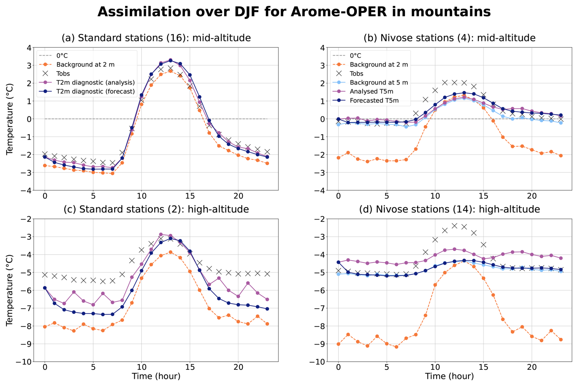
Figure 8Diurnal cycles of temperature observed (Tobs, crosses) or calculated at different steps within the assimilation workflow of Arome-OPER for mid-altitude mountain stations (a, b) and high-altitude mountain stations (c, d) over the study period. Within each altitude range a distinction is made between standard stations (a, c) and Nivose stations (b, d). The number of stations is given in brackets. Within the modeled temperatures, the background at 2 m (orange) refers to the Arome background interpolated at the observation point (dashed orange box in Fig. 3); the background at 5 m (light blue) designates the background at the first level of the model at the closest grid point of the station; the forecast temperature comes from the Arome-OPER forecast (see Sect. 2.4, navy blue line) also taken at the closest grid point of the station; and the analyzed T5m (or T2m diagnostic – analysis) in purple refers to the T5m analysis (or its associated T2m diagnostic) accounting for all observations including surface and satellite ones.
When examining the situation at Nivose stations (Fig. 8b and d), the background at 2 m used in the 3DVar assimilation appears too cold compared to the observations. This is not surprising since the observations are at 5 m and observed temperatures are, on average, warmer at 5 m than at 2 m, and the model is negatively and increasingly biased for T2m from 1600 m a.s.l to high altitudes (cf. Sect. 3.1). In relation to this, Fig. 8 consistently shows that the background at 2 m is colder at high altitudes than at mid-altitudes.
Secondly, we note that at Nivose stations, the analyzed T5m performs poorly at night, and especially worse than the forecast at 5 m (at middle and high altitudes), and even then the background at 5 m (at high altitudes) (Fig. 8b and d) has a warm bias of up to 0.9 °C at 07:00 UTC for high-altitude stations, whereas the 5 m background and forecasts are almost unbiased. This means that the assimilation of the observations leads to an overcorrection of T5m in the model, which switches from underestimation in the forecast and background at high altitudes to overestimation in the analysis. This error is consistent with the fact that the height of the Nivose stations is not being taken into account in the assimilation, as theoretically assessed in the previous section. In fact, the value of the innovation (observation minus background) at high-altitude Nivose stations would be much lower at night if it was calculated correctly using the background at 5 m: the mean innovation at night (from 18:00 to 07:00 UTC) would then be +0.1 °C compared to +3.8 °C when calculated with the background at 2 m as currently done. This analysis alone cannot prove that the misaccounting for the height of Nivose measurements is the sole source of errors, as other observations are assimilated within the 3DVar to produce the analyzed T5m; however, the results shown in Fig. 8 are fully compatible with our hypotheses.
During daytime at high altitudes, the forecast temperatures at 5 m (Fig. 8d) and at 2 m (Fig. 8c) are too cold with a maximum diurnal bias of −2.0 °C at 12:00 UTC for the Nivose stations and −1.8 °C at 08:00 UTC for the standard stations; both biases are partly corrected by the analysis. We hypothesize that the lower magnitude of the innovation during that part of the day, and possibly the contribution of other observation sources (satellite, etc.), prevents an overcorrection of the analyzed T5m as seen at night. Note that for technical reasons, the interpolation procedure for the background temperature at 2 m involves the four nearest grid points to the station and differs from that used for the other model products (nearest model grid point). This induces a structural difference between the background at 2 m and, for instance, the forecast at 2 m that is usually below 0.5 °C but can be enhanced by local effects when only a few stations are considered like in Fig. 8c, resulting in that case in the background at 2 m being distinctively colder than the forecast at that height.
In mid-altitude mountain areas, the analyzed T5m is also worse than the forecast at Nivose stations at night, a degradation consistent with an overestimated increment of about +2.0 °C for the background at 2 m at night that would have been reduced to about +0.1 °C if considered at 5 m (Fig. 8b). However, the effects are less marked at these mid-altitude Nivose stations than at the high-altitude ones because the T5m–T2m difference is smaller (cf. Sect. 3.2.1). In addition, the mid-altitude areas are more influenced by the standard stations (with no problematic sensor height) than the high-altitude ones, where stations are scarcer and mostly Nivose. The effect of height error should therefore be more limited in mid-altitude mountains. In conclusion, the assimilation of screen-level temperature observations degrades the analyzed T5m at the point closest to the Nivose stations, especially at night. This predominantly affects the high-altitude areas, as the height problem is less prominent at lower altitudes and affects fewer observation stations. However, at standard stations, the assimilation generally leads to an improvement in the temperature forecast at night without any deterioration during the day (Fig. 8b and d), which conforms with the expectations of an assimilation system.
3.3 Effect of geographic heterogeneities within the mountain observation network on the 3DVar assimilation
We performed targeted assimilation experiments to estimate the impact of two problems present in the Arome-OPER assimilation system (cf. Sect. 2.4):
-
The heterogeneity in density and altitudinal coverage of the observation network by means of the NO_VALLEY experiment.
-
The altitude mismatch between the stations and model grid points by means of the 150M experiment.
These two problems are present in Arome-OPER but not in 150M and NO_VALLEY, respectively. By comparing the improvement brought about by assimilation with respect to its background (i.e., the analysis increment) between Arome-OPER and the experiments, we can quantify the impact of these problems, particularly in relation to the contribution of upper-air and surface observations. Although the experiments do not make any difference in their assimilation between station types, in order to be able to compare their analysis increments with the observations, we will separate the Nivose from the standard stations in our results.
3.3.1 Quantifying the impact of altitude differences between stations and model grid (150M experiment)
In our dataset, there are 13 weather stations (out of 82) for which the model relief (of the grid point containing the station) differs by more than 150 m from the station's actual altitude. These 13 stations are therefore not assimilated in the 150M experiment.
Figure 9 shows that relief errors have only a weak effect on assimilation at all attitudes: the analysis increment calculated without the surface stations impacted by an error of more than 150 m between model relief and station altitude (“relief error” in the legend) differs at most by only a few tenths of a degree from the analysis increment including all surface stations, which is not significant in relation to the observation error. Our results also confirm that in valleys, this error has no impact, but this is not surprising since only one station out of 46 exhibits a relief mismatch with respect to the model.
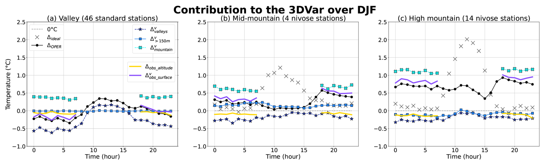
Figure 9Analysis increments (denoted Δ) obtained in different configurations of the pool of assimilated observations, as described in Sect. 2.4.2. These increments are retrieved at station locations in valleys (a), mid-altitude mountains (b), and high-altitude, taking into account only Nivose stations in mountains (b, c). The difference between the observation and the background of Arome-OPER represents an idealized increment (black crosses). There is no measure at 5 m in valleys, so no idealized increment is calculated.
Stations with unrealistic relief represent a small proportion of mountain observations in the French Alps (15 %), which likely explains this small effect. In fact, there are 2 Nivose stations out of 4 in the mid-altitude mountains and 2 out of 14 at high altitudes. There are more standard stations with a relief mismatch, with 7 out of 16 in mid-altitude mountains and 1 out of 2 at high altitudes.
Even if we focus on the diurnal cycle of assimilation at the station, the difference between Arome-OPER and 150M remains negligible and has a sign that varies and is decorrelated from the altitude. Furthermore, this difference does not depend on the sign and value of the difference between the model relief and reality. Thus, although significant differences can occasionally be observed between 150M and Arome-OPER, we conclude that stations with an important altitude mismatch with respect to the model have a negligible impact on assimilation in Arome.
3.3.2 Quantifying the impact of the altitudinal heterogeneity in station density (NO_VALLEY experiment)
As stated in the Introduction, the 3DVar assimilation system does not consider any effect of the topography. Valley stations therefore influence the analysis calculated for mid-altitude and high-altitude mountains, and vice versa, disregarding the differences in dominant processes and model biases across altitudes, highlighted for instance in Sect. 3.1. By comparing the analysis increments between the NO_VALLEY and Arome-OPER experiments (cf Sect. 2.4.2), we can quantify the impact of lowland and valley stations on the analyzed T5m at higher altitudes.
Figure 9 shows that the assimilation of lowland and valley stations has a cooling effect at all altitudes. Their impact is the most important and significant in the lowlands and Alpine valleys, where nighttime cooling averages −0.4 °C with a minimum of −0.7 °C at 06:00 UTC (Fig. 9a). In the mid-altitude mountains, the impact is weaker with a maximum contribution of −0.3 °C at 06:00 UTC. The assimilation of lowland and valley stations also cools the high altitudes by −0.3 °C on average (Fig. 9c) at night at Nivose stations.
Similarly, we can examine the contribution of the mountain (mid-altitude and high-altitude) observations at night through the NO_VALLEY analysis increment. On average, their contribution to assimilation amounts to +0.3 °C in the valleys (cyan line in Fig. 9a). At mid-altitudes, mountain observations warm the assimilation at Nivose stations by 0.6 °C (Fig. 9b). At high altitudes, this warming is greater, with a mean contribution of 1.1 °C (Fig. 9c). Mountain stations therefore warm the analysis at nighttime, whatever the altitude of the stations, even in the valleys.
It hence appears that the nighttime cooling effect of (numerous) valley stations on the analyzed T5m in mountains has the same magnitude as the nighttime warming effect of (scarcer) mountain stations on the analyzed T5m in valleys. However, the assimilation of mountain stations has a stronger effect in mountain areas than the assimilation of flatland and valley stations there, which have an effect of opposite sign (cooling) and a magnitude 2 times (for mid-altitudes) to 4 times (for high altitudes) lower. This result suggests that the heterogeneity in station density across altitudes has a moderate but not dominant impact in shaping the screen-level temperature analysis increment in high-altitude regions.
4.1 Impact of mountain, surface, and altitude observations on assimilation
Mountain stations contribute to positive assimilation increments at night in mid- and high-altitude mountains, ranging from 0.6 to 1.1 °C in mean values (Sect. 3.3.2). In high altitudes and to a lesser extent in mid-altitudes, this warming overnight degrades the performance of Arome-OPER, as illustrated by a distinctively positive assimilation increment, while the ideal increment is close to zero. The results of the assimilation experiments hence confirm the results from Sect. 3.2 and the role of mountain station assimilation in the degradation of the T5m analysis.
As the Arome-OPER T5m forecast bias is very weak at night at high altitudes (Fig. 8), we deduce that the positive increment of the analysis comes in part from the comparison of the (colder) model T2m diagnostic with the Nivose observations taken at about 5 m over the surface. Another source of error is the direct use of the temperature increment at 2 m to modify the model temperature at 5 m, without a transfer to the correct height above the surface to calculate the analyzed temperature at the first level of the model. These two influences have not yet been individually quantified. The first problem is included in the mountain contribution (cyan line, Fig. 9), while the second affects all surface observations.
As mentioned in Sect. 3.3.2, we note that the contribution of valley stations to the analysis increment in mountains dampens the warming effect of the assimilation of mountain stations by about 0.3 °C. This negative contribution is an artifact of the 3DVar system that does not account for relief in the spatial area of influence of the increments, but it has the effect of limiting the warm bias of the analyzed T5m at Nivose stations. Therefore it can be seen as a compensation error within the model.
Finally, our assimilation experiments enable an insight into the role of surface vs. upper-air observation assimilation across altitudes in mountain regions. The contribution of the surface observations is, by construction, the composition of the mountain and valley contributions. At night, surface observations cool the valleys by −0.1 °C on average, as the negative contribution of valley observations is higher in magnitude than the positive contribution of mountain observations (Fig. 9a). This helps reduce the warm bias of Arome in valleys (Fig. 6). The aggregated effect of surface observations is opposite in mid- and high-altitude mountains, where they warm the T5m analysis more significantly (Fig. 9b and c) due to a high positive and dominant contribution of mountain stations over valley stations.
In mid-altitude areas, the contribution of surface observations reaches +0.6 °C at 18:00 UTC at Nivose stations. At high altitudes, the contribution of surface observations is higher, with an average nighttime contribution of 0.85 °C at Nivose stations. These positive analysis increments are in line with the dominant role of mountain station assimilation for altitude regions and the height-above-surface and missing adjoint issues mentioned above. Conversely, altitude observations warm the valleys by an average of 0.1 °C, with a maximum of 0.5 °C at 01:00 UTC, and cool the mountains by −0.1 °C. We conclude that in mountain regions, the assimilation of T5m is therefore mainly influenced by surface observations throughout all altitudes: from valleys to high mountains. Most strikingly, at least for the nighttime period, the analysis increment due solely to altitude (upper-air) observations is closer to the ideal increment than those induced by surface observations alone and by Arome-OPER. This suggests that, at least for nighttime conditions, the assimilation of surface observations as a whole is not beneficial for the analysis of T5m at middle and high altitudes.
4.2 Main findings and insights into the use of temperature observations in mountains
Our study examined the impacts of inhomogeneities in the surface observation network in complex, mountainous alpine terrain on the evaluation of the performances of a numerical weather prediction system and on the assimilation of these data themselves. The inhomogeneities studied are of three flavors: (i) the difference in height above the surface of the temperature sensors across altitudes, in connection with the development of the snowpack over the winter; (ii) the difference of altitude between the individual observation stations and the model grid point they are located in; and (iii) the inhomogeneity in station densities between valleys and mountaintops.
We find that the various heights above the surface of the measurements involved across altitudes matter. First, as significant differences exist in a number of meteorological situations where temperatures differ between 2 m height and further up above the surface in high-mountain regions, this difference impacts targeted model evaluations. Second, the NWP or atmospheric models may present quite different biases at different heights above the surface, even within a few meters. In the example of the Arome system, our distinction between 5 and 2 m across the observational network enables us to state that the temperature at the lowest model prognostic level, close to 5 m above the surface, is only very moderately biased in Arome. However, temperature proves highly biased at levels below, be it at 2 m above the surface or more intensely directly at the surface itself. This generalizes the findings of Gouttevin et al. (2023) based on a two-site study in the French Alps and makes the T2m temperature bias as much of a concern for surface modelers as for atmospheric ones. We therefore recommend that model biases be analyzed as at different heights, considering the proper height of the measurements available, as illustrated in Figs. 6 and 7.
In the case of Arome, we further found that these differences in biases at different heights lead to an overestimation of the assimilation increment when the differences in height are not accounted for in the assimilation system and 5 m high observations are assimilated as 2 m high ones. As a result, while useful for the correction of near-surface air temperatures for the initial (analysis) step of forecasts in low-altitude regions (Leuenberger et al., 2024), the assimilation of surface stations is actually currently detrimental in mountain regions in the French high-resolution weather forecasting system. We also note that activating the adjoint of the diagnostic within the assimilation could be a first step to reduce the current errors in the assimilation process.
Contrarily, we find that the relief mismatch between stations and the model has no significant impact in assimilation. This conclusion may be relative to the configuration of stations where this mismatch is observed in the present case study, only 15 % of which present an important mismatch with respect to the relief of the Arome-OPER system, that runs with a high spatial resolution coming with an enhanced representation of the topography. It should be verified when working with coarser model resolutions or in other mountain regions. In particular, it may not hold for regions with more abrupt relief and more intense altitude variations like the Himalayas.
With regards to the heterogeneous density of stations across altitudes, our study shows that the valleys and lower-altitude stations that are the most numerous and hence the most assimilated in the French Alps have a lower influence on the analysis of temperature at high-altitude areas than the high-altitude stations themselves. This result suggests that the topographic heterogeneity in station density has a moderate impact on high-altitude regions. Again, this conclusion is not general and should be revisited in other regions or even for specific regions of the French Alps with lower station densities.
As a matter of fact, in the present case study, the effect of low-altitude stations at high-altitude locations and the effect of high-altitude station assimilation on the temperature of low-altitude areas have the same order of magnitude, changing the analysis temperature by about ±0.3 °C. However, these effects are of opposite signs: this means that data from a different altitude bring a moderate but non-null correction to the model at another altitude, where the biases can be different and hence be enhanced instead of corrected. In the case of Arome, the assimilation of valley stations warms the model at high altitudes, while the assimilation of high-altitude stations, relevant for high-altitude model behavior, tends to cool it. This result illustrates the limitations of the current 3DVar assimilation system that disregards the effect of topography in the spatial structure of assimilation increments. To prevent these undesirable effects, topography should be better accounted for in the assimilation systems. So Merker et al. (2018) have shown that the KENDA (Km-scale ENsemble-based Data Assimilation) system (Schraff et al., 2016) used in COSMO better catches small-scale features like orography (Schraff et al., 2016). For Arome, an ensemble assimilation scheme (3DEnvar, Brousseau et al., 2025) was recently introduced in the new operational version. This scheme implicitly accounts for relief via background error correlation matrices inferred from the model ensemble. This new feature could help reduce the impact of inhomogeneity in station densities between valleys and mountaintops.
In line with previous studies, our work here highlights that model biases differ significantly across altitudes (Rudisill et al., 2024; Vionnet et al., 2016; Quéno et al., 2016; Monteiro et al., 2022). Therefore, we strongly recommend that different altitude regions should be considered separately or differently in assimilation (see above) but also when it comes to model evaluation. Only evaluation differentiated by altitude can foster a better understanding of the model limitations and promote efficient model improvements over mountain regions, targeting altitude-specific biases and underlining processes. For instance, in the case of Arome, the awareness of a concomitant high-altitude cold and low-altitude warm bias can lead to the hypothesis of deficient katabatic flows that provide a convenient explanatory mechanism discussed in more detail in Sect. 4.3. Such a hypothesis could not have been formulated if only one global bias had been assessed without altitudinal differentiation.
Similarly, we estimate that not considering the height-above-surface difference between standard and Nivose stations has long impeded a proper quantification and understanding of the near-surface temperature bias of our NWP system, Arome, probably partly hindering its resolution. Having a more accurate T2m estimate, not affected by, e.g., the error in measurement height, would enable better knowledge of the true model biases and the formulation of relevant hypotheses for these biases, henceforth favoring the improvement of the model's physical parameterizations. For example, in the case of Arome-OPER, the accuracy of the temperature representation at the lowest model level enables us to mostly exclude problems linked to the dynamical core of the atmospheric model and to draw the focus on the surface energy balance and associated processes. Some further examples of hypotheses will be described in Sect. 4.3.
4.3 Towards a more robust surface temperature
Figure 4a and b show a different behavior of the modeled surface temperature Ts according to altitude. At the high-altitude site CLB, where the surface is rock generally covered with snow in winter, the Ts is too cold by several degrees (up to −7 °C negative bias at night) in winter, and the diurnal cycle is too strong. This cold bias in Ts has a direct impact on the diagnostic of T2m. On the other hand, at the mid-altitude CDP site, where the surface is grassy and surrounded by a forest environment and snow cover can be discontinuous in winter, the Ts modeled by Arome is too warm (up to +4 °C positive bias during the day), while the diurnal cycle remains too strong.
The thermal amplitude of the diurnal cycles of Ts is reported in Table 4 for both sites, showing this overestimation. It also has consequences for T2m that are diagnosed in part based on the surface temperature, as can be seen in Table 1.
Table 4Thermal amplitude of surface temperature observed and modeled by Arome-OPER at CDP and CLB over the winters (DJF) between 1 January 2020 and 28 February 2022.
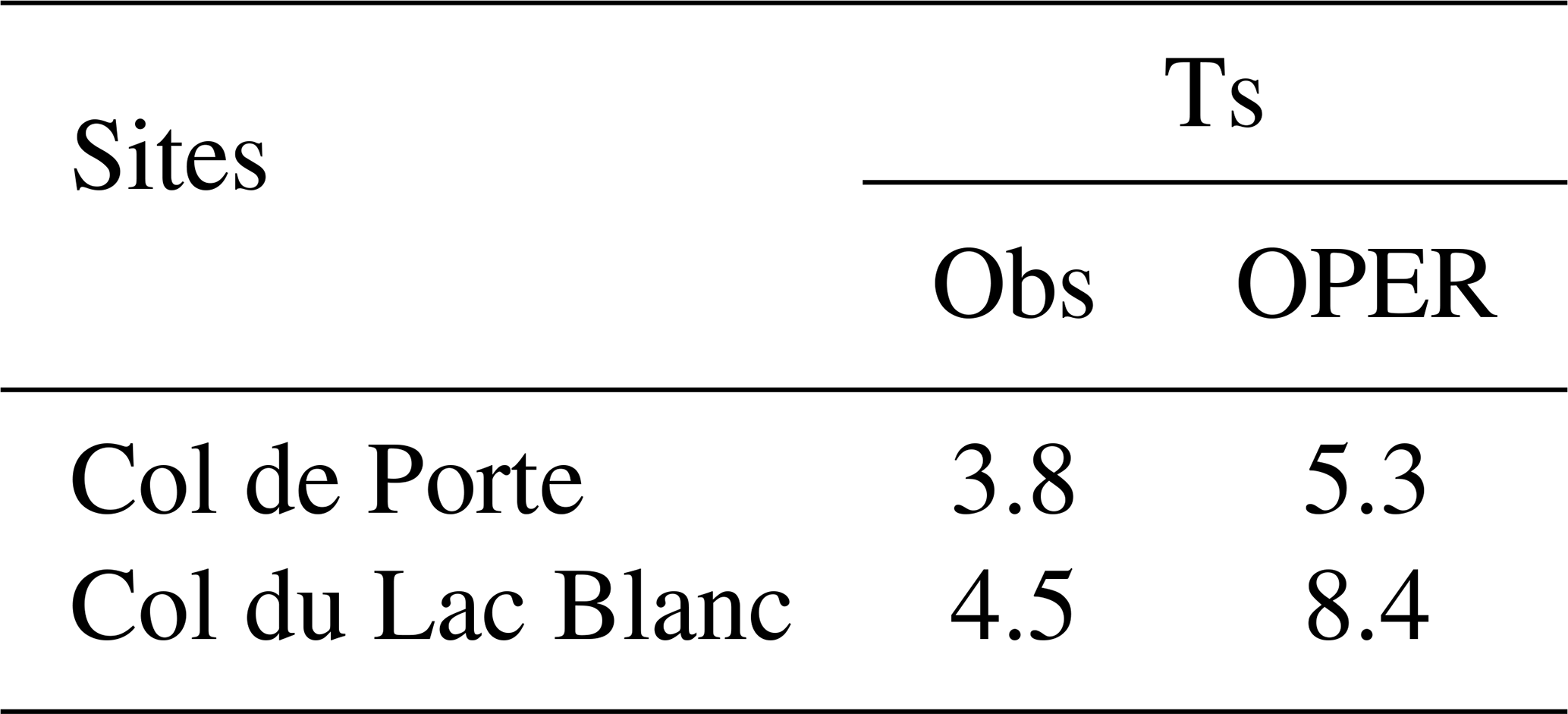
Hence, at the high-altitude site, the T2m nighttime negative bias of Arome is partly induced by a snow surface temperature that is too cold, an issue already highlighted by Gouttevin et al. (2023) and Monteiro et al. (2022) for this model, while other authors advance a clear imbrication between surface temperature, surface processes, and T2m biases for other models, especially in the presence of snow (e.g., Arduini et al., 2019; Rudisill et al., 2024). The surface processes possibly involved in these biases are manyfold: as snow rarely covers the ground thoroughly at the scale of a model grid cell, snow cover fractions are used by the models, with parameterizations rarely constrained by field data or suited to the local context of model application (Lalande et al., 2023). They constitute a first possible cause for surface temperature biases, as they are used to weight the surface energy fluxes over snow-covered and snow-free areas (Lalande et al., 2023; Liu et al., 2017). The representation of the snow cover is also often pinpointed as a possible source of surface and near-surface temperature biases, in connection with processes like the thermal conduction (one-layered snow model being unable to account for the thermal conductivity and low thermal inertial of surface snow layers) or albedo (possibly in connection with the snow cover fraction) (Arduini et al., 2019; Rudisill et al., 2024).
In the case of the Arome-OPER system specifically, the ground scheme currently used relies on a force-restore approach (the Isba-3L surface scheme) and a one-layered snow model (D95) with a single soil–vegetation–snow surface temperature relationship, a configuration pinpointed by several authors for excessive winter nighttime cooling at the surface of the snowpack (Etchevers, 2000; Douville et al., 1995; Gouttevin et al., 2023; Monteiro et al., 2022). One avenue of research is to replace the present force-restore scheme with a multilayer soil and surface scheme, Isba-DIFF, that allows a resolution of specific energy balances for the soil–vegetation system as described in Monteiro et al. (2024) and would be associated with the multilayer snow scheme Isba-ES (Boone and Etchevers, 2001). These changes that promote a more physical representation of the soil–snow–atmosphere continuum have been successfully tested by Monteiro et al. (2024) with modifications to improve the snow cover.
Deficiencies in the turbulent coupling between the surface and the atmosphere over snow are another very likely source of the cold bias in surface and screen-level temperatures. The situations of strong stability often encountered over continuous snowpacks at high altitudes in low wind conditions tend to reduce the turbulent transfer coefficient between the surface and atmosphere and, therefore, to decouple the surface from the atmosphere in the models, leading to excessive surface cooling. The turbulent exchanges in mountain regions are hard to capture by atmospheric models, as the assumptions behind the Monin–Obukhov similarity theory implemented in the models are violated in complex terrain (e.g., Rotach et al., 2022). In the case of Arome, Gouttevin et al. (2023) showed that turbulent coupling was underestimated at nighttime during stable conditions at high altitudes, significantly contributing to the T2m cold bias. The turbulent coupling between snow and the atmosphere in complex terrain could be revisited along with the scientific progress in that field, and recent or ongoing work (Stiperski et al., 2019; Stiperski and Calaf, 2023; McCandless et al., 2022) may lead to interesting breakthroughs in the coming years. Also, we add as a note that katabatic winds are likely misrepresented in atmospheric models of kilometric scales like Arome due to a resolution in the lower atmosphere that is too coarse, i.e., within the few meters above the surface (Blein, 2016). The likely underestimation of their strength provides an interesting alternative explanatory mechanism for both the near-surface cold bias at high altitudes and warm bias in valleys, a hypothesis that we suggest here but that has yet to be verified against in situ data.
Finally, it would be interesting to have Ts measurements in Alpine valleys, as this warm bias could partly explain the T2m warm bias observed in valleys in winter and the model's difficulty in predicting cold pools.
4.4 T2m diagnostic ill-adapted to complex terrain?
While the more complex physical parameterizations could improve mountain temperature forecasting (as evoked in Sect. 4.3), it should be remembered that the T2m field produced by Arome as well as by most atmospheric models at kilometric scale or above is a diagnostic field (Rudisill et al., 2024; Ingleby et al., 2024). It is computed from the temperature at the lowermost model level, T5m, and the surface temperature, Ts, via an interpolation formula generally relying on the Monin–Obukhov similarity theory and depending on surface layer parameterizations, notably surface roughness lengths and stability corrections. In the case of Arome, this analytical formulation is established so as to ensure that the estimated static energy profile between the surface and a given height, here 2 m, is consistent with the modeled fluxes higher up, at the lowermost prognostic model level (Geleyn, 1988). Therefore, first, this diagnostic inherits the limitations exposed in Sect. 4.3 for the estimations of the turbulent fluxes in complex terrain and may be biased in highly stable, nocturnal conditions, just because the modeled fluxes are biased in these situations (see Sect. 4.3) Second, this diagnostic was developed at a time when the resolution of Arome's coupling model, Arpege (Bubnová et al., 1995), was of the order of 20 km over the Alps and relief was therefore less important in the model. Hence, while suitable for the boundary layer over the plains, it is likely not adapted to mountainous areas.
According to Serafin et al. (2018) and Arduini (2017), the boundary layer is complex in mountain areas. In the valleys, when high-pressure systems develop in winter, the winds are weak and cold air is trapped, forming cold pools, so that the vertical temperature profile shows a strong inversion extending vertically over several tens of meters and lasting sometimes throughout the day. At high altitude, however, the inversions will be strong in the very first few meters only and may frequently be less than 2 m thick. Figure 10 illustrates this situation, whereby the model features a temperature inversion that is too thick. In this case, the T2m diagnostic has a cold bias, induced both by a surface temperature that is too cold (see Sect. 4.3) and by an inversion that is not as shallow over the surface as in observations.
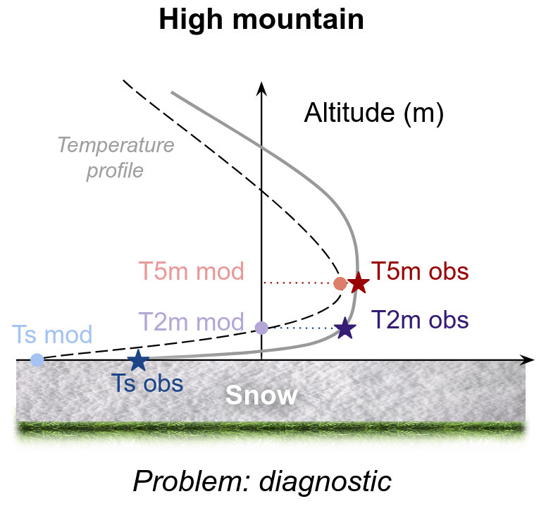
Figure 10This diagram illustrates the differences between the modeled temperature profile (black dotted line) and the actual profile (gray solid line) at high altitude in winter: the modeled surface temperature is too cold, and the layer over which the inversion develops is too thick, both leading to a cold bias at 2 m. Ts is in blue, T2m in purple, and T5m in red.
When a weather disturbance arrives, the cold air will remain trapped in the valleys for several hours, while the high altitude will be under the effect of synoptic-scale circulation. The processes are therefore different for near-surface temperatures between valleys, mid-altitude mountains, and high-altitude areas. The T2m diagnostic must therefore be adapted accordingly.
To overcome such issues and especially solve the problem of nighttime disconnection frequently encountered between surface and atmospheric models, a prognostic surface boundary layer scheme has been proposed by Masson and Seity (2009): Canopy. This scheme was shown to foster large improvements during stable, nighttime conditions and in mountain areas, where analytical laws and interpolation methods for the temperature profile frequently fail (Masson and Seity, 2009). It hence constitutes a very promising alternative to diagnostics.
Following this approach, Meier et al. (2021) proposed using this surface boundary layer scheme for their simulations of temperature with Arome at kilometric resolution over the mountains and valleys of the Austrian operational weather forecasting domain. However, these authors noticed persistent model biases for different locations in connection with the topography (e.g., valleys vs. mountaintops) that encouraged them to consider the information from higher (lower) canopy levels for mountaintops (valley). In the end, they propose weighting the canopy levels for the final T2m output depending on the local topography, giving more weight to higher canopy levels or even the free atmosphere for exposed, mountaintop grid points and more weight to lower canopy levels for grid points in narrow Alpine valleys. A parameter (inversion factor noted IFAC) which depends on the position in the relief (plain, valley, mountain) is added in Canopy. This can be seen as a pragmatic way to inject in the model the different behaviors of the mountain and valley boundary layers, described above. The results are promising. As a reminder, the surface boundary layer scheme Canopy, originally developed in Arome-France, is deactivated in the current version because it enhances the valley warm T2m bias, no doubt due to error compensation. It still constitutes an interesting perspective but the current valley bias has to be solved prior to the re-activation of this scheme.
Other alternatives lie in the improvements of the diagnostics themselves, and some recent studies have proposed work in this direction. For instance, Dian and Masek (2016) proposed a modification to the T2m diagnostic from Geleyn (1988) using a different assumption for the structure function, but it is only suitable for stable or anticyclonic cases and did not improve the estimation of T2m in all topographic and weather situations. For their part, Ingleby et al. (2024) have also proposed a revision of T2m diagnostics in the IFS model that leads to less divergence from the theory and a more realistic evolution of T2m in stably stratified conditions.
Another final possibility would be to increase the number of vertical levels in the model in order to obtain a prognostic rather than a diagnostic temperature at 2 m. Indeed, recent work by Antoine et al. (2023) showed that adding levels in the lowermost layers of an atmospheric model significantly improves fog forecasting, thanks to a better representation of near-surface atmospheric variables. We hypothesize that having a first atmospheric level at around 2.5 m like in their study could therefore improve the representation of the vertical temperature profile in the first few meters of the atmosphere. This could typically be tested using the 500 m research version of Arome over the Alps, which has 120 vertical levels, with an increased number of levels near the surface (Arnould et al., 2021). All these perspectives may be investigated in the future for the Arome-OPER NWP system.
This study investigated the impact of inhomogeneities of the observational network specific to mountain regions on the evaluation of the NWP system Arome and on the effects of surface data assimilation within this system.
We first questioned whether the differences in height above the surface between sensors should be accounted for when evaluating models in terms of near-surface air temperature. These differences are correlated with altitude and induced by the need to prevent the sensors from being buried in thick snowpacks in high-altitude terrain over the winter. We showed that T5m and T2m should not be considered equivalent when performing model evaluations: despite a limited mean difference over winter at our mid- and high-altitude research sites, both temperatures can differ significantly in specific situations, especially low winds and clear skies. Therefore, taking one for another introduces errors. Furthermore, at the instance of the Arome model, atmospheric models may present very different biases at these different heights so that the confusion between the two temperatures leads to erroneous interpretations of model biases. We therefore recommend a distinct evaluation of modeled T5m and T2m against the relevant observations in mountain terrain. Only evaluation differentiated by altitude can foster a better understanding of the model limitations and promote efficient model improvements over mountain regions.
We then questioned whether this difference in height plays a detrimental role in assimilation, as observations at 2 or 5 m are not discriminated within the assimilation system of Arome, an approximation that we estimate may be common among NWP systems. We showed that, indeed, this confusion between heights in the assimilation process leads in the case of Arome to an overestimation of the analysis increment in high-altitude regions, inducing an overestimation of T5m analysis at night and a degradation of performances with respect to the model without assimilation (background or forecast), while relying on upper-air data (satellite, radar) assimilation only would produce a better analysis.
Finally, we questioned the effect of station vs. model relief mismatch and higher density in valley stations on the assimilation. The differences in altitude between stations and model grid points do not significantly affect the performance of assimilation, a result that is hard to generalize to other mountain regions or NWP systems as it likely depends on station densities across altitudes and model resolution. Similarly, we quantified the density imbalance between valley and mountain stations as not having a dominant effect on assimilation results, despite a non-null contribution from stations from distinct altitude ranges featuring different model biases and hence of limited relevance, on the order or 0.3 °C.
To summarize, this study helped define guidelines for the improvement of high-resolution NWP systems in mountain terrains: in particular, sensor height should be considered both in model evaluation and assimilation, topography should be accounted for in the spatial structure functions involved in assimilation, and model biases at 2 m height and lower could possibly be reduced by the use of diagnostics more appropriate to mountain terrain, a higher number of vertical levels in the models, and enhanced work on the surface scheme to improve the representation of soil–snow–atmosphere energy transfers.
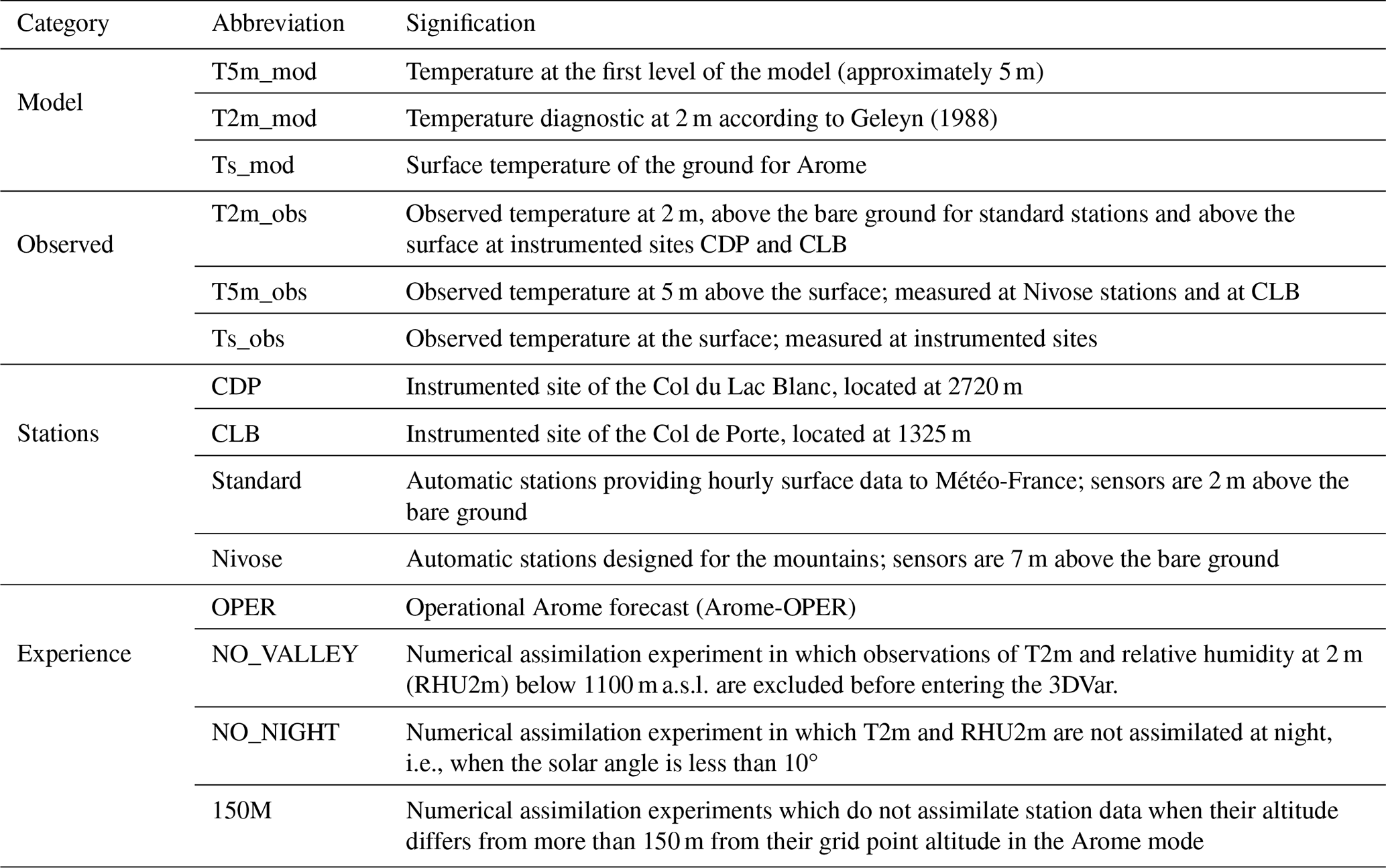
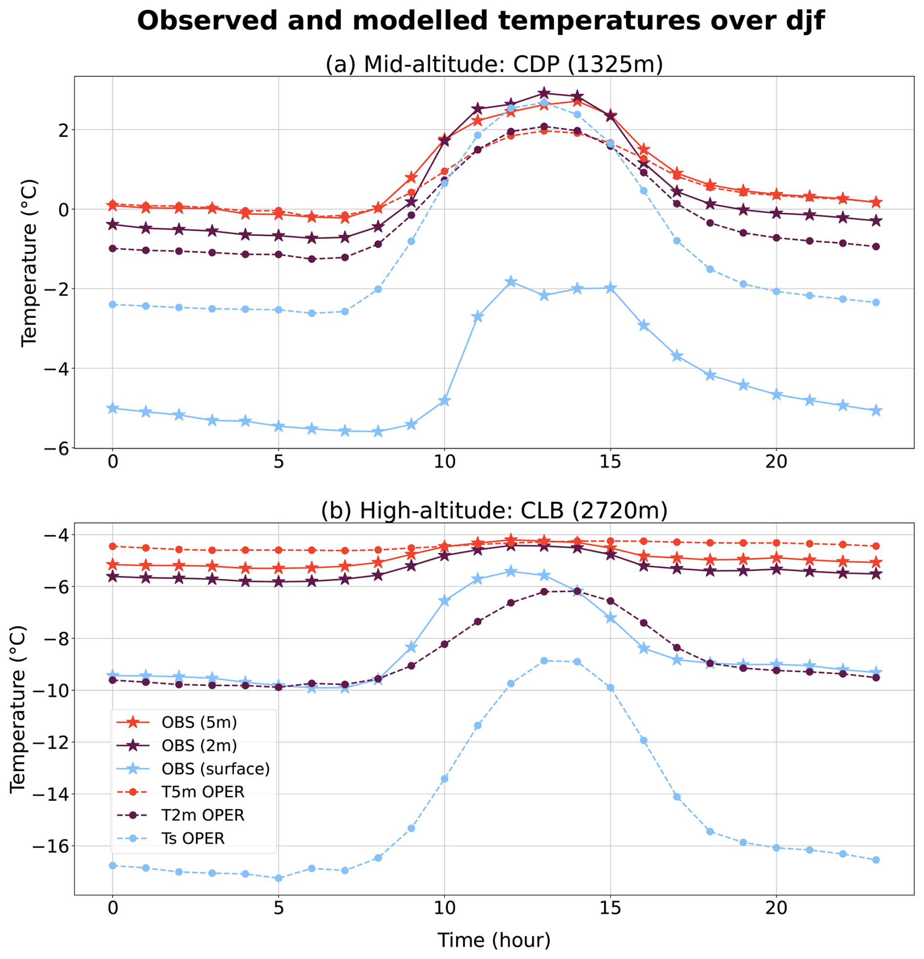
Figure B1Diurnal cycle of the 5 m, 2 m, and surface observed (OBS) and modeled (OPER) temperatures averaged over the winters of the study period at the CDP and CLB research sites.
The code used for the assimilation experiments in Arome-France is owned by the members of the ACCORD consortium. This agreement allows each member of the consortium to license the shared ACCORD codes to academic institutions in their home countries for non-commercial research. Access to codes used for the figures can be obtained by contacting the corresponding author. The main data from the Col du Lac Blanc and Col de Porte instrumented sites are available at https://doi.osug.fr/public/ (last access: 27 October 2025) (GLACIOCLIM-CLB, 2024; GLACIOCLIM_CDP, 2023). Complementary data for the CLB used in the present paper, namely the interpolated 2 and 5 m temperatures and surface temperature computed using incoming longwave radiation, have been made available here: https://doi.org/10.5281/zenodo.14989735 (GLACIOCLIM-CLB, 2025). Data from the Météo-France surface observation network and from the operational Arome-FRANCE model (analyses and forecasts) are freely available at https://portail-api.meteofrance.fr/web/en/ (last access: 27 October 2025) (Météo-France, 2025). Data from the numerical experiments performed within this study are available at https://doi.org/10.5281/zenodo.16570743 (Préaux, 2025). All computations were performed with Python software version 3.12.3. The codes handling the station data and the numerical assimilation experiment are available from a Zenodo repository (https://doi.org/10.5281/zenodo.16570743; Préaux, 2025). It notably includes the scripts for the following tasks: performing all data preprocessing, reading the different data sources, statistical analyses leading to the tables, and plotting the figures.
DP carried out the numerical experiments, analyzed the results, and wrote the core of the manuscript. IDE, IG, and YS contributed to the design of the numerical experiments and helped DP analyze the results and write the manuscript.
The contact author has declared that none of the authors has any competing interests.
Publisher’s note: Copernicus Publications remains neutral with regard to jurisdictional claims made in the text, published maps, institutional affiliations, or any other geographical representation in this paper. While Copernicus Publications makes every effort to include appropriate place names, the final responsibility lies with the authors. Views expressed in the text are those of the authors and do not necessarily reflect the views of the publisher.
The authors are grateful to Camille Birman, Pierre Brousseau, and Matthieu Plu for proofreading the article, to Hugo Merzisen for his help with the CDP and CLB data, and to Patrick Moll for his insights on assimilation.
This research has been supported by the French Meteorological Institute Météo-France. The Col du Lac Blanc and Col de Porte instrumented sites are part of the OZCAR Research Infrastructure through the GLACIOCLIM Observatory. They receive financial support from the OSUG LabEx OSUG@2020 (grant ANR10 LABX56), Météo-France, and INRAE.
This paper was edited by Cenlin He and reviewed by two anonymous referees.
Antoine, S., Honnert, R., Seity, Y., Vié, B., Burnet, F., and Martinet, P.: Evaluation of an improved AROME configuration for fog forecasts during the SOFOG3D campaign, Weather and Forecasting, 38, 1605–1620, https://doi.org/10.1175/WAF-D-22-0215.1, 2023. a
Arduini, G.: Processus de la couche limite atmosphérique stable hivernale en vallée alpine, phdthesis, 2017. a
Arduini, G., Balsamo, G., Dutra, E., Day, J. J., Sandu, I., Boussetta, S., and Haiden, T.: Impact of a multi-layer snow scheme on near-surface weather forecasts, Journal of Advances in Modeling Earth Systems, 11, 4687–4710, 2019. a, b
Arnould, G. and Préaux, D.: Study of AROME Temperature in mountain regions, ACCORD Newsletter, https://www.umr-cnrm.fr/accord/IMG/pdf/accord-nl1.pdf (last access: 27 October 2025), 2021. a
Arnould, G., Dombrowski-Etchevers, I., Gouttevin, I., and Seity, Y.: Améliorer la prévision de température en montagne par des descentes d’échelle, La Météorology, 115, 37–44, https://doi.org/10.37053/lameteorologie-2021-0091, 2021. a, b
Atlaskin, E. and Vihma, T.: Evaluation of NWP results for wintertime nocturnal boundary-layer temperatures over Europe and Finland, Quarterly Journal of the Royal Meteorological Society, 138, 1440–1451, 2012. a
Aymoz, G., Jaffrezo, J. L., Chapuis, D., Cozic, J., and Maenhaut, W.: Seasonal variation of PM10 main constituents in two valleys of the French Alps. I: EC/OC fractions, Atmos. Chem. Phys., 7, 661–675, https://doi.org/10.5194/acp-7-661-2007, 2007. a
Beauvais, L.: Fronts chauds sur les Alpes : Hiver 2017–2018. Comportement des modèles, Ateliers de la prévision du Centre-Est, 2018. a, b, c
Becken, S.: The importance of climate and weather for tourism: literature review, Lincoln University, LEaP, https://researcharchive.lincoln.ac.nz/entities/publication/72cdf0e5-5933-44cb-906b-3575c7125129 (last access: 27 October 2025), 2010. a
Blein, S.: Observation et modélisation de couche limite atmosphérique stable en relief complexe: le processus turbulent d'écoulement catabatique, PhD thesis, Université Grenoble Alpes, https://theses.hal.science/tel-01622676 (last access: 27 October 2025), 2016. a
Boone, A. and Etchevers, P.: An Intercomparison of Three Snow Schemes of Varying Complexity Coupled to the Same Land Surface Model: Local-Scale Evaluation at an Alpine Site, Journal of Hydrometeorology, 2, 374–394, 2001. a
Brousseau, P., Seity, Y., Ricard, D., and Léger, J.: Improvement of the forecast of convective activity from the AROME-France system, Q. J. Roy. Meteor. Soc., 142, 2231–2243, https://doi.org/10.1002/qj.2822, 2016. a, b, c, d
Brousseau, P., Vogt, V., Arbogast, E., Martet, M., Thomas, G., and Berre, L.: The operational 3DEnVar data assimilation scheme for the Météo-France convective scale model AROME-France, EGUsphere [preprint], https://doi.org/10.5194/egusphere-2025-2642, 2025. a
Bubnová, R., Hello, G., Bénard, P., and Geleyn, J.-F.: Integration of the fully elastic equations cast in the hydrostatic pressure terrain-following coordinate in the framework of the ARPEGE/Aladin NWP system, Mon. Weather Review, 123, 515–535, https://doi.org/10.1175/1520-0493(1995)123<0515:IOTFEE>2.0.CO;2, 1995. a, b
Chow, F. K., De Wekker, S. F., and Snyder, B. J.: Mountain weather research and forecasting: recent progress and current challenges, vol. 750, Springer, ISBN 9789400740976, 2013. a
Courtier, P. and Geleyn, J.-F.: A global numerical weather prediction model with variable resolution: Application to the shallow-water equations, Quarterly Journal of the Royal Meteorological Society, 114, 1321–1346, 1988. a
Demortier, A., Mandement, M., Pourret, V., and Caumont, O.: Assimilation of surface pressure observations from personal weather stations in AROME-France, Nat. Hazards Earth Syst. Sci., 24, 907–-927, https://doi.org/10.5194/nhess-24-907-2024, 2024. a, b
Deng, X. and Stull, R.: Assimilation of surface observations in complex terrain, in: Ninth Symposium on Integrated Observing and Assimilation Systems for the Atmosphere, Oceans, and Land Surface, San Diego, 9–14 January 2025, https://ams.confex.com/ams/Annual2005/techprogram/paper_86561.htm (last access: 27 October 2025), 2005. a
Dian, M. and Masek, J.: Improving the Computation of Screen Level Fields (Temperature, Moisture), Report of LACE Stay at CHMI in Prague 11–29 April 2015, 2015, Prague, https://www.rclace.eu/File/Physics/2016/dian_screeninter_pragueApr2016.pdf (last access: 27 October 2025), 2016. a
Dombrowski-Etchevers, I., Vionnet, V., and Quéno, L.: Pertinence des prévisions météorologiques à l'échelle kilométrique pour la modélisation du manteau neigeux en montagne, La Météorologie, p. 25, https://doi.org/10.4267/2042/63587, 2017. a, b, c, d, e, f, g, h, i, j
Douville, H., Royer, J. F., and Mahfouf, J. F.: A new snow parameterization for the Météo-France climate model: Part I: validation in stand-alone experiments, Clim. Dynam., 12, 21–35, https://doi.org/10.1007/BF00208760, 1995. a, b
Dozier, J. and Warren, S. G.: Effect of viewing angle on the infrared brightness temperature of snow, Water Resources Research, 18, 1424–1434, 1982. a
Durand, Y., Brun, E., Merindol, L., Guyomarc'h, G., Lesaffre, B., and Martin, E.: A meteorological estimation of relevant parameters for snow models, Annals of Glaciology, 18, 65–71, 1993. a
Etchevers, P.: Modélisation du cycle continental de l'eau à l'échelle régionale. Impact de la modélisation de la neige sur l'hydrologie du Rhône, PhD thesis, https://theses.hal.science/tel-00466802 (last access: 27 October 2025), 2000. a
Fischer, C., Bouyssel, F., Brousseau, P., El Khatib, R., Pottier, P., Seity, Y., Wattrelot, E., and Joly, A.: Les modèles opérationnels de prévision numérique à aire limitée de Météo-France, La Météorologie, 2018, 18–28, https://doi.org/10.4267/2042/65139, 2018. a
Geleyn, J.-F.: Interpolation of wind, temperature and humidity values from model levels to the height of measurement, Tellus A, 40, 347–351, 1988. a, b, c, d
Giard, D. and Bazile, E.: Implementation of a new assimilation scheme for soil and surface variables in a global NWP model, Monthly Weather Review, 128, 997–1015, https://doi.org/10.1175/1520-0493(2000)128<0997:IOANAS>2.0.CO;2, 2000. a, b
GLACIOCLIM_CDP: Col de Porte: a meterological and snow observatory, OSUG [data set], https://doi.osug.fr/public/CRYOBSCLIM_CDP/ (last access: 30 July 2024), 2023. a
GLACIOCLIM-CLB: Col du Lac Blanc: a meteorological and blowing snow observatory, OSUG [data set], https://doi.osug.fr/public/CRYOBSCLIM_CLB/ (last access: 18 July 2024), 2024. a
GLACIOCLIM-CLB: Col du Lac Blanc: additional data, Zenodo [data set], https://doi.org/10.5281/zenodo.14989735, 2025. a
Gouttevin, I., Langer, M., Löwe, H., Boike, J., Proksch, M., and Schneebeli, M.: Observation and modelling of snow at a polygonal tundra permafrost site: spatial variability and thermal implications, The Cryosphere, 12, 3693–3717, https://doi.org/10.5194/tc-12-3693-2018, 2018. a
Gouttevin, I., Vionnet, V., Seity, Y., Boone, A., Lafaysse, M., Deliot, Y., and Merzisen, H.: To the origin of a wintertime screen-level temperature bias at high altitude in a kilometric NWP model, Journal of Hydrometeorology, 24, 53–71, https://doi.org/10.1175/JHM-D-21-0200.1, 2023. a, b, c, d, e, f, g, h, i
Guillet, O.: Modélisation des corélations spatiales d'erreurs d'observation en assimilation de données variationnelle: étude sur des maillages non structurés, PhD thesis, Institut National Polytechnique de Toulouse-INPT, https://theses.hal.science/tel-04160718v1 (last access: 27 October 2025), 2019. a, b
Gustafsson, N., Janjić, T., Schraff, C., Leuenberger, D., Weissmann, M., Reich, H., Brousseau, P., Montmerle, T., Wattrelot, E., Bučánek, A., Mile, M., Hamdi, R., Lindskog, M., Barkmeijer, J., Dahlbom, M., Macpherson, B., Ballard, S., Inverarity, G., Carley, J., Alexander, C., Dowell, D., Liu, S., Ikuta, Y., and Fujita, T.: Survey of data assimilation methods for convective-scalenumerical weather prediction at operational centres, Q. J. Roy. Meteor. Soc., 144, 1218–1256, https://doi.org/10.1002/qj.3179, 2018. a, b
Guyomarc'h, G., Bellot, H., Vionnet, V., Naaim-Bouvet, F., Déliot, Y., Fontaine, F., Puglièse, P., Nishimura, K., Durand, Y., and Naaim, M.: A meteorological and blowing snow data set (2000–2016) from a high-elevation alpine site (Col du Lac Blanc, France, 2720 m a.s.l.), Earth Syst. Sci. Data, 11, 57–69, https://doi.org/10.5194/essd-11-57-2019, 2019. a, b, c
Ingleby, B., Arduini, G., Balsamo, G., Boussetta, S., Ochi, K., Pinnington, E., and de Rosnay, P.: Improved two-metre temperature forecasts in the 2024 upgrade, ECMWF Newsletter, https://www.ecmwf.int/en/newsletter/178/earth-system-science/improved-two-metre-temperature-forecasts-2024-upgrade (last access: 27 October 2025), 2024. a, b
Jörg-Hess, S., Griessinger, N., and Zappa, M.: Probabilistic forecasts of snow water equivalent and runoff in mountainous areas, Journal of Hydrometeorology, 16, 2169–2186, https://doi.org/10.1175/JHM-D-14-0193.1, 2015. a
Kotlarski, S., Lüthi, D., and Schär, C.: The elevation dependency of 21st century European climate change: an RCM ensemble perspective, International Journal of Climatology, 35, https://doi.org/10.1002/joc.4254, 2015. a
Lac, C., Chaboureau, J.-P., Masson, V., Pinty, J.-P., Tulet, P., Escobar, J., Leriche, M., Barthe, C., Aouizerats, B., Augros, C., Aumond, P., Auguste, F., Bechtold, P., Berthet, S., Bielli, S., Bosseur, F., Caumont, O., Cohard, J.-M., Colin, J., Couvreux, F., Cuxart, J., Delautier, G., Dauhut, T., Ducrocq, V., Filippi, J.-B., Gazen, D., Geoffroy, O., Gheusi, F., Honnert, R., Lafore, J.-P., Lebeaupin Brossier, C., Libois, Q., Lunet, T., Mari, C., Maric, T., Mascart, P., Mogé, M., Molinié, G., Nuissier, O., Pantillon, F., Peyrillé, P., Pergaud, J., Perraud, E., Pianezze, J., Redelsperger, J.-L., Ricard, D., Richard, E., Riette, S., Rodier, Q., Schoetter, R., Seyfried, L., Stein, J., Suhre, K., Taufour, M., Thouron, O., Turner, S., Verrelle, A., Vié, B., Visentin, F., Vionnet, V., and Wautelet, P.: Overview of the Meso-NH model version 5.4 and its applications, Geosci. Model Dev., 11, 1929–1969, https://doi.org/10.5194/gmd-11-1929-2018, 2018. a
Lafore, J. P., Stein, J., Asencio, N., Bougeault, P., Ducrocq, V., Duron, J., Fischer, C., Héreil, P., Mascart, P., Masson, V., Pinty, J. P., Redelsperger, J. L., Richard, E., and Vilà-Guerau de Arellano, J.: The Meso-NH Atmospheric Simulation System. Part I: adiabatic formulation and control simulations, Annales Geophysicae, 16, 90–109, 1998. a
Lalande, M., Ménégoz, M., Krinner, G., Ottlé, C., and Cheruy, F.: Improving climate model skill over High Mountain Asia by adapting snow cover parameterization to complex-topography areas, The Cryosphere, 17, 5095–5130, https://doi.org/10.5194/tc-17-5095-2023, 2023. a, b
Lejeune, Y., Dumont, M., Panel, J.-M., Lafaysse, M., Lapalus, P., Le Gac, E., Lesaffre, B., and Morin, S.: 57 years (1960–2017) of snow and meteorological observations from a mid-altitude mountain site (Col de Porte, France, 1325 m of altitude), Earth Syst. Sci. Data, 11, 71–88, https://doi.org/10.5194/essd-11-71-2019, 2019. a
Leuenberger, D., Merker, C., Chandramouli, K., Crezee, B., and Arpagaus, M.: Benefit and challenges in assimilating near-surface temperature and humidity observations in complex terrain. in: 8th WMO workshop on the Impacts of Various Observing Systems on Numerical Weather Prediction and Earth System Prediction, 27–30 May 2024, Norrköping, Sweden, https://cgms-info.org/wp-content/uploads/2024/12/8th-Impact_Workshop-Final_Report.pdf (last access: 27 October 2025), 2024. a
Liu, C., Ikeda, K., Rasmussen, R., Barlage, M., Newman, A. J., Prein, A. F., Chen, F., Chen, L., Clark, M., Dai, A., Dudhia, J., Eidhammer, T., Gochis, D., Gutmann, E., Kurkute, S., Li, Y., Thompson, G., and Yates, D.: Continental-scale convection-permitting modeling of the current and future climate of North America, Climate Dynamics, 49, 71–95, 2017. a
Mahfouf, J.-F., Brasnett, B., and Gagnon, S.: A Canadian precipitation analysis (CaPA) project: Description and preliminary results, Atmosphere-Ocean, 45, 1–17, 2007. a
Marimbordes, S., Birman, C., Arbogast, E., Fourrié, N., and Mahfouf, J.-F.: Towards a 2DEnVar surface data assimilation approach within the convective scale numerical weather prediction model AROME-France, Quarterly Journal of the Royal Meteorological Society, 150, 5225–5248, 2024. a, b, c
Masson, V. and Seity, Y.: Including Atmospheric Layers in Vegetation and Urban Offline Surface Schemes, Journal of Applied Meteorology and Climatology, 48, 1377–1397, https://doi.org/10.1175/2009JAMC1866.1, 2009. a, b
Masson, V., Le Moigne, P., Martin, E., Faroux, S., Alias, A., Alkama, R., Belamari, S., Barbu, A., Boone, A., Bouyssel, F., Brousseau, P., Brun, E., Calvet, J.-C., Carrer, D., Decharme, B., Delire, C., Donier, S., Essaouini, K., Gibelin, A.-L., Giordani, H., Habets, F., Jidane, M., Kerdraon, G., Kourzeneva, E., Lafaysse, M., Lafont, S., Lebeaupin Brossier, C., Lemonsu, A., Mahfouf, J.-F., Marguinaud, P., Mokhtari, M., Morin, S., Pigeon, G., Salgado, R., Seity, Y., Taillefer, F., Tanguy, G., Tulet, P., Vincendon, B., Vionnet, V., and Voldoire, A.: The SURFEXv7.2 land and ocean surface platform for coupled or offline simulation of earth surface variables and fluxes, Geosci. Model Dev., 6, 929–960, https://doi.org/10.5194/gmd-6-929-2013, 2013. a
McCandless, T., Gagne, D. J., Kosović, B., Haupt, S. E., Yang, B., Becker, C., and Schreck, J.: Machine learning for improving surface-layer-flux estimates, Boundary-Layer Meteorology, 185, 199–228, 2022. a
Meier, F., Wastl, C., Weidle, F., and Wittmann, C.: Adapting the screening level diagnostics to improve AROME temperature forecasts in Alpine areas, ACCORD Newsletter, https://www.umr-cnrm.fr/accord/IMG/pdf/accord-nl1.pdf (last access: 27 October 2025), 2021. a
Merker, C., Leuenberger, D., Anlauf, H., Potthast, R., and Arpagaus, M.: Additive covariance inflation in KENDA: Towards a climatological error covariance matrix from COSMO, in: 20th COSMO GM, edited by: MeteoSwiss, St. Petersburg, Russia, https://www.cosmo-model.org/content/consortium/generalMeetings/general2018/parallel/additiveInflation_merker.pdf (last access: 27 October 2025), 2018. a
Monteiro, D., Caillaud, C., Samacoïts, R., Lafaysse, M., and Morin, S.: Potential and limitations of convection-permitting CNRM-AROME climate modelling in the French Alps, International Journal of Climatology, 42, 7162–7185, https://doi.org/10.1002/joc.7637, 2022. a, b, c, d, e, f, g, h
Monteiro, D., Caillaud, C., Lafaysse, M., Napoly, A., Fructus, M., Alias, A., and Morin, S.: Improvements in the land surface configuration to better simulate seasonal snow cover in the European Alps with the CNRM-AROME (cycle 46) convection-permitting regional climate model, Geosci. Model Dev., 17, 7645–7677, https://doi.org/10.5194/gmd-17-7645-2024, 2024. a, b
Morin, S., Lejeune, Y., Lesaffre, B., Panel, J.-M., Poncet, D., David, P., and Sudul, M.: An 18-yr long (1993–2011) snow and meteorological dataset from a mid-altitude mountain site (Col de Porte, France, 1325 m alt.) for driving and evaluating snowpack models, Earth Syst. Sci. Data, 4, 13–21, https://doi.org/10.5194/essd-4-13-2012, 2012. a, b
Morin, S., Horton, S., Techel, F., Bavay, M., Coléou, C., Fierz, C., Gobiet, A., Hagenmuller, P., Lafaysse, M., Ližar, M., Mitterer, C., Monti, F., Müller, K., Olefs, M., Snook, J.S., van Herwijnen, A., and Vionnet, V.: Application of physical snowpack models in support of operational avalanche hazard forecasting: A status report on current implementations and prospects for the future, Cold Regions Science and Technology, 170, 102910, https://doi.org/10.1016/j.coldregions.2019.102910, 2020. a
Météo-France: Météo France data, https://portail-api.meteofrance.fr/web/en/ (last access: 18 July 2024), 2025. a
Naaim-Bouvet, F. and Truche, M.: Guide technique “Ouvrages à vent en zone de montagne”, in: International Snow Science Workshop (ISSW), Irstea, ANENA, Meteo France, 134 pp., https://hal.science/hal-00949755/document (last access: 27 October 2025), 2013. a
Noilhan, J. and Planton, S.: A simple parameterization of land surface processes for meteorological models, Mon. Weather Rev., 117, 536–549, https://doi.org/10.1175/1520-0493(1989)117<0536:ASPOLS>2.0.CO;2, 1989. a
Paci, A., Staquet, C., Allard, J., Barral, H., Canut, G., Cohard, J.-M., Jaffrezo, J.-L., Martinet, P., Sabatier, T., Troude, F., Arduini, G., Burnet, F., Brun, C., Chemel, C., Dabas, A., Donier, J.-M., Garrouste, O., Guillot, R., Largeron, Y., Legain, D., Maurel, W., Tzanos, D., Barrau, S., Barret, M., Barrie, J., Belleudy, A., Bouhours, G., Bourrianne, T., Chevrier, F., Douffet, T., Etcheberry, J.-M., Gustave, L., Mazoyer, M., Mercier, S., Moulin, E., Pellan, Y., Piguet, B., Rodier, Q., and Zin, I.: La campagne Passy-2015: dynamique atmosphérique et qualité de l’air dans la vallée de l’Arve, American Institute of Physics Melville, NY, https://doi.org/10.4267/pollution-atmospherique.5903, 2016. a, b, c
Peixóto, J. P. and Oort, A. H.: Physics of climate, Reviews of Modern Physics, 56, 365, https://doi.org/10.1103/RevModPhys.56.365, 1984. a
Pepin, N. and Kidd, D.: Spatial temperature variation in the Eastern Pyrenees, Weather, 61, 300–310, https://doi.org/10.1256/wea.106.06, 2006. a
Pichelli, E., Coppola, E., Sobolowski, S., Ban, N., Giorgi, F., Stocchi, P., Alias, A., Belušić, D., Berthou, S., Caillaud, C., Cardoso, R. M., Chan, S., Christensen, O. B., Dobler, A., de Vries, H., Goergen, K., Kendon, E. J., Keuler, K., Lenderink, G., Lorenz, T., Mishra, A. N., Panitz, H-J., Schär, C., Soares, P. M. M., Truhetz, H., and Vergara-Temprado, J.: The first multi-model ensemble of regional climate simulations at kilometer-scale resolution part 2: historical and future simulations of precipitation, Climate Dynamics, 56, 3581–3602, 2021. a
Préaux, D.: codes and dataset of numerical assimilation experiments, Zenodo [code and data set], https://doi.org/10.5281/zenodo.16570743, 2025. a, b
Quéno, L., Vionnet, V., Dombrowski-Etchevers, I., Lafaysse, M., Dumont, M., and Karbou, F.: Snowpack modelling in the Pyrenees driven by kilometric-resolution meteorological forecasts, The Cryosphere, 10, 1571–1589, https://doi.org/10.5194/tc-10-1571-2016, 2016. a, b, c
Rotach, M. W., Serafin, S., Ward, H. C., Arpagaus, M., Colfescu, I., Cuxart, J., De Wekker, S. F., Grubišic, V., Kalthoff, N., Karl, T., Kirshbaum, D. J., Lehner, M., Mobbs, S., Paci, A., Palazzi, E., Bailey, A., Schmidli, J., Wittmann, C., Wohlfahrt, G., and Zardi, D.: A collaborative effort to better understand, measure, and model atmospheric exchange processes over mountains, Bulletin of the American Meteorological Society, 103, E1282–E1295, 2022. a
Rudisill, W., Rhoades, A., Xu, Z., and Feldman, D. R.: Are atmospheric models too cold in the mountains? The state of science and insights from the SAIL field campaign, Bulletin of the American Meteorological Society, 105, E1237–E1264, https://doi.org/10.1175/BAMS-D-23-0082.1, 2024. a, b, c, d, e, f, g, h, i, j
Scherrer, S., Ceppi, P., Croci-Maspoli, M., and Appenzeller, C.: Snow-albedo feedback and Swiss spring temperature trends, Theoretical and Applied Climatology, 110, 509–516, 2012. a
Schraff, C., Reich, H., Rhodin, A., Schomburg, A., Stephan, K., Perianez, A., and Potthast, R.: Kilometre-scale ensemble data assimilation for the COSMO model (KENDA), Quarterly Journal of the Royal Meteorological Society, 142, 1453–1472, 2016. a, b
Seity, Y., Brousseau, P., Malardel, S., Hello, G., Bénard, P., Bouttier, F., Lac, C., and Masson, V.: The AROME-France Convective-Scale Operational Model, Mon. Weather Rev., 139, 976–991, https://doi.org/10.1175/2010MWR3425.1, 2011. a
Serafin, S., Adler, B., Cuxart, J., De Wekker, S. F. J., Gohm, A., Grisogono, B., Kalthoff, N., Kirshbaum, D. J., Rotach, M. W., Schmidli, J., Stiperski, I., Večenaj, Z., and Zardi, D.: Exchange Processes in the Atmospheric Boundary Layer Over Mountainous Terrain, Atmosphere, 9, https://doi.org/10.3390/atmos9030102, 2018. a
Sheridan, P., Vosper, S., and Smith, S.: A Physically Based Algorithm for Downscaling Temperature in Complex Terrain, Journal of Applied Meteorology and Climatology, 57, 1907–1929, https://doi.org/10.1175/JAMC-D-17-0140.1, 2018. a
Spandre, P., François, H., George-Marcelpoil, E., and Morin, S.: Panel based assessment of snow management operations in French ski resorts, Journal of Outdoor Recreation and Tourism, 16, 24–36, https://doi.org/10.1016/j.jort.2016.09.002, 2016. a
Stiperski, I. and Calaf, M.: Generalizing Monin-Obukhov similarity theory (1954) for complex atmospheric turbulence, Physical Review Letters, 130, 124001, https://doi.org/10.1103/PhysRevLett.130.124001, 2023. a
Stiperski, I., Calaf, M., and Rotach, M. W.: Scaling, anisotropy, and complexity in near-surface atmospheric turbulence, Journal of Geophysical Research: Atmospheres, 124, 1428–1448, 2019. a
Sturm, M. and Liston, G. E.: Revisiting the global seasonal snow classification: An updated dataset for earth system applications, Journal of Hydrometeorology, 22, 2917–2938, 2021. a
Taillefer, F.: CANARI Some technical features, in: NetFAM working days, edited by: Météo-France, Oslo, Sweden, https://netfam.fmi.fi/OBS09/Taillefer_1.pdf (last access: 27 October 2025), 2009. a
Thornton, J. M., Pepin, N., Shahgedanova, M., and Adler, C.: Coverage of in situ climatological observations in the world's mountains, Frontiers in Climate, 4, 814181, https://doi.org/10.3389/fclim.2022.814181, 2022. a
Torma, C., Giorgi, F., and Coppola, E.: Added value of regional climate modeling over areas characterized by complex terrain – Precipitation over the Alps, Journal of Geophysical Research: Atmospheres, 120, 3957–3972, 2015. a
Van Hyfte, S.: Mise en oeuvre et évaluation d'un nouveau système de réanalyses météorologiques des paramètres de surface à haute résolution, PhD thesis, Institut National Polyetchnique de Toulouse – INPT, https://theses.hal.science/tel-04186752 (last access: 27 October 2025), 2021. a
Vernay, M., Lafaysse, M., Monteiro, D., Hagenmuller, P., Nheili, R., Samacoïts, R., Verfaillie, D., and Morin, S.: The S2M meteorological and snow cover reanalysis over the French mountainous areas: description and evaluation (1958–2021), Earth Syst. Sci. Data, 14, 1707–1733, https://doi.org/10.5194/essd-14-1707-2022, 2022. a
Vionnet, V., Guyomarc’h, G., Bouvet, F. N., Martin, E., Durand, Y., Bellot, H., Bel, C., and Puglièse, P.: Occurrence of blowing snow events at an alpine site over a 10-year period: Observations and modelling, Advances in Water Resources, 55, 53–63, 2013. a
Vionnet, V., Bélair, S., Girard, C., and Plante, A.: Wintertime subkilometer numerical forecasts of near-surface variables in the Canadian Rocky Mountains, Monthly Weather Review, 143, 666–686, 2015. a, b
Vionnet, V., Dombrowski-Etchevers, I., Lafaysse, M., Quéno, L., Seity, Y., and Bazile, E.: Numerical Weather Forecasts at Kilometer Scale in the French Alps: Evaluation and Application for Snowpack Modeling, Journal of Hydrometeorology, 17, 2591–2614, https://doi.org/10.1175/JHM-D-15-0241.1, 2016. a, b, c, d, e, f, g, h, i, j, k, l, m, n, o, p
Vionnet, V., Fortin, V., Gaborit, E., Roy, G., Abrahamowicz, M., Gasset, N., and Pomeroy, J. W.: Assessing the factors governing the ability to predict late-spring flooding in cold-region mountain basins, Hydrol. Earth Syst. Sci., 24, 2141–2165, https://doi.org/10.5194/hess-24-2141-2020, 2020. a
Whiteman, C. D.: Mountain meteorology: fundamentals and applications, Oxford University Press, https://doi.org/10.1093/oso/9780195132717.001.0001, 2000. a
Winstral, A., Jonas, T., and Helbig, N.: Statistical downscaling of gridded wind speed data using local topography, Journal of Hydrometeorology, 18, 335–348, https://doi.org/10.1175/JHM-D-16-0054.1, 2017. a
Winter, K. J. P. M., Kotlarski, S., Scherrer, S. C., and Schär, C.: The Alpine snow-albedo feedback in regional climate models, Climate Dynamics, 48, 1109–1124, 2017. a
- Abstract
- Introduction
- Material and methods
- Results
- Discussion
- Conclusions
- Appendix A: Summary of key abbreviations used in the study
- Appendix B: Diurnal cycles of surface, screen-level, and 5 m temperatures at the Col de Porte and Col du Lac Blanc sites
- Code and data availability
- Author contributions
- Competing interests
- Disclaimer
- Acknowledgements
- Financial support
- Review statement
- References