BOSSE v1.0: the Biodiversity Observing System Simulation Experiment

As global and regional vegetation diversity loss threatens essential ecosystem services under climate change, monitoring biodiversity dynamics and its role in ecosystem services is crucial in predicting future states and providing insights into climate adaptation and mitigation. In this context, remote sensing (RS) offers a unique opportunity to assess long-term and large-scale biodiversity dynamics. However, the development of this capability suffers from the lack of consistent, global, and spatially matched ground diversity measurements that enable testing and validating generalizable methodologies. The Biodiversity Observing System Simulation Experiment (BOSSE) aims to alleviate the lack of this information by means of simulation. BOSSE simulates synthetic landscapes featuring communities of various vegetation species whose traits's seasonality and ecosystem functions (e.g., biospheric fluxes) respond to meteorology and environmental factors. Simultaneously, BOSSE can generate various types of remote sensing imagery linked to the traits and functions via radiative transfer theory. Specifically, it simulates hyperspectral reflectance factors (R), which can be convolved to the bands of specific RS missions, sun-induced chlorophyll fluorescence (SIF), and land surface temperature (LST). The resolution of the RS imagery can be degraded to test the robustness of different approaches to information loss and the capability of new methodologies to overcome this limitation. Therefore, BOSSE enables users to evaluate the capability of different methods to estimate plant functional diversity (PFD) from RS and link it to ecosystem functions. We expect BOSSE to support the benchmarking and improvement of old and novel methods dedicated to estimating plant diversity and exploring the biodiversity–ecosystem function (BEF) relationships, facilitating advances in this growing area of research and supporting the analysis and interpretation of real-world measurements. We also expect BOSSE to be extended and include new features that provide more realistic simulations that help answer more complex questions related to climate change and global warming.

1 Introduction

Climate change and other human-induced environmental changes jeopardize ecosystems' biodiversity and functions, many of which directly translate to ecosystem services (Hernández-Blanco et al., 2022). Biodiversity can sustain the stability of ecosystem functions, such as photosynthesis or transpiration, in response to environmental variability, perturbations, and extreme events (Mahecha et al., 2024; de Bello et al., 2021). Many terrestrial ecosystem functions and services depend on plant diversity, as plants are the primary producers in terrestrial ecosystems, i.e., they produce the chemical components that support other living beings (Isbell et al., 2011). Therefore, it is necessary to establish a system for global plant diversity monitoring to assess and quantify biodiversity loss, sustain ecosystem stability, and forecast future scenarios (Gonzalez et al., 2023; Pereira et al., 2013). In this context, remote sensing (RS, find a glossary in Table A for all the terms not defined in other tables) has become a valuable tool, given its capability to provide continuous and synoptic information on the Earth's surfaces (Cavender-Bares et al., 2017). Since the proposition of the Spectral Variation Hypothesis (SVH) (Palmer et al., 2000), the spatial variability of spectral signals and RS products has been related to different facets of vegetation diversity, such as taxonomic (Van Cleemput et al., 2023), functional (Ma et al., 2019), and phylogenetic (Schweiger et al., 2018) diversity; moreover, recent works have also linked RS-derived diversity with ecosystem functional properties (Gomarasca et al., 2024). However, other studies have also reported RS failing to capture different facets of plant diversity, at least in particular cases (Ludwig et al., 2024; Fassnacht et al., 2022; Van Cleemput et al., 2023).

The evaluation of the SVH is challenging since the test outcome strongly depends on the data used (e.g., field sampling schemes, sensor features, and resolutions), the methodologies and metrics quantifying diversity, and the type and extent of the study sites. The variability and lack of overlap of these factors lead to a broad spectrum of results (Torresani et al., 2024), which are not systematically comparable. Since most studies are limited in all these aspects, it remains unclear whether the hypothesis should be discarded or whether the methods and data fail to capture plant diversity. The underlying problem is a lack of consistent global databases (meaning representative of the Earth's terrestrial ecosystems) to develop, compare, and identify reliable methodologies. Furthermore, the relationships established between RS and field estimates of plant diversity are often indirect due to a lack of physical connection between the variables measured in the field and the spectral signals of vegetation. This lack of connection limits the interpretation and generalization of the results and might make the estimation of some diversity facets unreliable and context-dependent (e.g., taxonomic diversity; Fassnacht et al., 2022). Among all the diversity facets, plant functional diversity (PFD) is the most directly (physically) linked to RS data since it relies on the physical properties of vegetation that determine its interaction with radiation. However, not all traits or their measurements feature this physical link. For example, ecological surveys often measure plant traits on a per-leaf mass basis, which are less connected to the spectral signals captured by RS than if measured per-leaf area (Kattenborn et al., 2019). In addition, the effect of the measurement uncertainties and spatial mismatches between field and RS data is poorly understood and could induce spurious relationships and conclusions (Pacheco-Labrador et al., 2022). Consequently, despite multiple studies (for a literature review, see Torresani et al., 2024), basic methodological questions remain unanswered, and there is a risk that methodologies prone to spuriousness are identified as adequate and others more suitable pass unnoticed.

Generating consistent datasets for robust methodological benchmarking and SVH evaluation would require great coordination efforts and dedicated field sampling protocols rarely used by ecologists or remote sensing scientists. On the one hand, the plant traits targeted by ecologists (characteristics of organisms that influence performance or fitness), along with their sampling schemes, are not optimized for evaluating RS-based estimates of biophysical variables or their diversity. On the other hand, adapting the typical sampling schemes in RS to facilitate the evaluation of diversity estimates could require both n-folding the sampling effort (e.g., multiplying the number of sampling plots to build n-by-n grids as in Hauser et al., 2021) and making sure that the variables (traits) that significantly influence the spectral signals are effectively measured. Furthermore, optimized samplings should be applied in research stations where ecosystem functions are also measured so that methods to assess BEF relationships using remote sensing -a nascent research field- can be robustly developed. Nowadays, even the most promising coordinated activities in this direction (Barnett et al., 2019) lack sampling protocols fully optimized for testing the SVH and benchmarking RS methods, despite which these efforts are extremely valuable.

Alternatively, some researchers have used radiative transfer models to overcome the lack of suitable field datasets (simulating them instead) and answer methodological questions regarding the capability of RS to infer different plant taxonomic (Badourdine et al., 2023; Fassnacht et al., 2022; Van Leeuwen et al., 2021) and functional diversity (Pacheco-Labrador et al., 2022; Ludwig et al., 2024). Simulations have also helped to understand the results found using RS data to assess BEF relationships (Gomarasca et al., 2024). Within the limitations of the synthetic data, these works have provided valuable insights into methodological questions and framed the chances of RS to infer plant diversity within wide ranges of situations that exceed those covered by local and individual studies. Radiative transfer simulations have also helped to test new diversity metrics optimized for RS data (Pacheco-Labrador et al., 2023). However, these works have been relatively limited regarding the simulation of multiple spectral signals, the incorporation of phenology, the spatial representation of landscapes, the corresponding RS imagery, and the connection of spectral signals with ecosystem functions.

This manuscript presents the Biodiversity Observing System Simulation Experiment (BOSSE), a modeling tool to advance the development of RS methods to monitor PFD and BEF relationships from space. BOSSE simulates 1) spatially explicit scenes (vegetation-populated landscapes) where plant traits (PT) and the associated functions (e.g., biospheric fluxes) respond to meteorology and environmental factors, and 2) the physically and physiologically connected imagery of hyperspectral reflectance factors (R), sun-induced chlorophyll fluorescence radiance (F), land surface temperature (LST), and retrieved optical traits (OT). BOSSE v1.0 is designed to benchmark metrics and methods that cope with the challenges of using RS data to capture PFD and relate the PFD estimates with ecosystem functions in space and time, allowing for a flexible configuration of the simulations, e.g., degrading sensor resolutions while always providing a reference or best-case scenario. We expect BOSSE to help the RS community benchmark and develop their methods in a controlled environment, supporting the interpretation and design of experiments and measurements.

2 Methods

2.1 BOSSE model

The BOSSE model v1.0 is a spatially defined dynamic vegetation model able to simulate maps of plant traits, functions (e.g., biospheric fluxes), and the physically and physiologically connected remote sensing imagery in the optical domain at hourly steps. It allows various configuration options that enable repeatable simulations featuring different spatial patterns, climatic and meteorological conditions, taxonomic richness, spatial and temporal resolutions, or simulated satellite missions. A BOSSE “Scene” is a configurable synthetic landscape containing species' individuals whose properties and functions evolve in response to meteorology and other spatially varying environmental conditions (e.g., soil properties). BOSSE conceives a plant “species” as a classification rather than an evolutionary unit (Dupré, 2001). A species is defined as a unique set of variables (phenological maximum and minimum radiative transfer variables and phenological model parameters, among others) that is randomly generated. Moreover, BOSSE simulates intra-specific variability so that each species represents the averaged specific phenotype and response to the environment (phenology) of a group of individuals. Consequently, in the simulated plant traits maps, each pixel shows unique values that differ to some degree from the values of the pixels corresponding to the same species. This variability propagates to the spectral signals and functions related to each pixel. Despite operating on a continuous trait space, each species is associated with a given plant functional type (PFT), which constrains the range of variability and sometimes the covariance between traits and the relative abundance as a function of the simulated Köppen climatic zone.

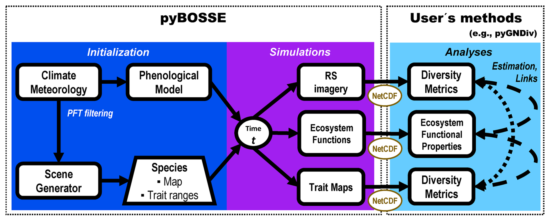
Figure 1 Biodiversity Observing System Simulation Experiment (BOSSE) workflow. First, the BOSSE model is initialized for a particular scene where the climatic zone and local meteorology limit the plant functional types (PFT) present. Then, the model is able to simulate plant trait maps, ecosystem functions, and remote sensing (RS) imagery at any desired time of the meteorological time series. From these outputs, the users can apply any methods they choose to estimate diversity metrics and relate them to ecosystem functions.

Figure 1 summarizes BOSSE's workflow, which is divided into three phases (the last one, “Analyses”, is to be implemented by the user). BOSSE is coded in Python 3.11 as a Class to facilitate usability. The source code and a Jupyter tutorial are published on GitHub (https://github.com/JavierPachecoLabrador/pyBOSSE, last access: 10 June 2025) under the GPL-3 license.

Initialization of the BOSSE class. Each simulation location is assigned to a given climatic zone that determines the presence and the probability of occurrence of the different PFTs represented (S1 in the Supplement). Moreover, meteorological data time series (e.g., radiation, air temperature, soil moisture) are used with a phenological model to filter out the least competitive PFTs under those conditions. Then, one or more species are assigned to each PFT. The individuals of the different species are located in space, assuming each pixel is occupied by one individual or a group of identical individuals and, therefore, it contains a unique set of plant trait values. Then, the maximum and minimum values of all traits (i.e., radiative transfer variables) are defined for each pixel.

Simulation: Once BOSSE is initialized for a given Scene, the phenological model parameters and the trait ranges determine the trait values of each individual at any given time as a function of meteorology. The results of this step are plant trait maps and the corresponding RS imagery and ecosystem functions. These data can be directly analyzed with Python or stored in NetCDF files for later assessment with other programming languages or software. BOSSE also allows for estimating large-scale simulations' computational costs (in time) so that users can allocate the necessary resources.

Analyses: The user can use BOSSE outputs to compute functional diversity metrics from the simulated trait maps and the simulated RS imagery. It is also possible to derive ecosystem functional properties from the ecosystem functions. These products can be used to benchmark different methods and answer methodological questions (e.g., which variables capture the best plant diversity or BEF relationships). In this manuscript, we exemplify the analysis of BOSSE v1.0 outputs with the Python package “pyGNDiv” (https://github.com/JavierPachecoLabrador/pyGNDiv-master, last access: 10 June 2025) (Pacheco-Labrador et al., 2023) recently updated with “numba” (Lam et al., 2015) compilation for faster computation and new features to directly asses cubes of RS imagery, products or plant trait maps. pyGNDiv provides a selection of benchmarked functional diversity metrics and methods for partitioning diversity at different scales (Pacheco-Labrador et al., 2023; Pacheco-Labrador et al., 2022) such as Rao's quadratic entropy index Q_Rao (Botta-Dukát, 2005) and the fractions of α (f_α) and β-diversity (f_β) using a variance-based approach (Laliberté et al., 2020). In addition, pyGNDiv normalizes the value of the metrics by the number of variables so that these are comparable one-to-one, independently of the number of traits or spectral bands analyzed. At this stage, the users can also test and benchmark their own methods and metrics.

2.2 BOSSE data and data-driven submodels

BOSSE combines data and several models parametrized from different datasets or bibliographic references.

2.2.1 Plant functional types and climatic zones

We determined the relative abundance of different PFTs in each Köppen climatic zone by convolving the European Space Agency's Land Cover Climate Change Initiative (ESA LC-CCI) Global Plant Functional Types Dataset (v.2.08) from Harper et al. (2023) with the Köppen Climate Classification System maps from Rubel et al. (2017). We also considered the estimates of C3/C4 grass leaf area fraction generated in the NACP MsTMIP simulations (Global 0.5-degree Model Outputs in Standard Format, Version 2.0, from Huntzinger et al., 2021) to separate the Grasses PFTs (S1 in the Supplement). These probabilities are used to determine the number of species belonging to a PFT when a Scene is generated.

2.2.2 Meteorological data

For each climatic zone, we selected 15 random locations (60 sites total) where we downloaded two years (2020–2022) of ERA5-Land hourly meteorological data (S2 in the Supplement). Accumulated radiation was recomputed to instantaneous rates (W m⁻²) and accumulated precipitation at hourly intervals. The selected variables were prepared as the inputs of the model Soil Canopy Observation, Photochemistry and Energy fluxes (SCOPE) (Van Der Tol et al., 2009) as in Li et al. (2023) (Table S2 in the Supplement).

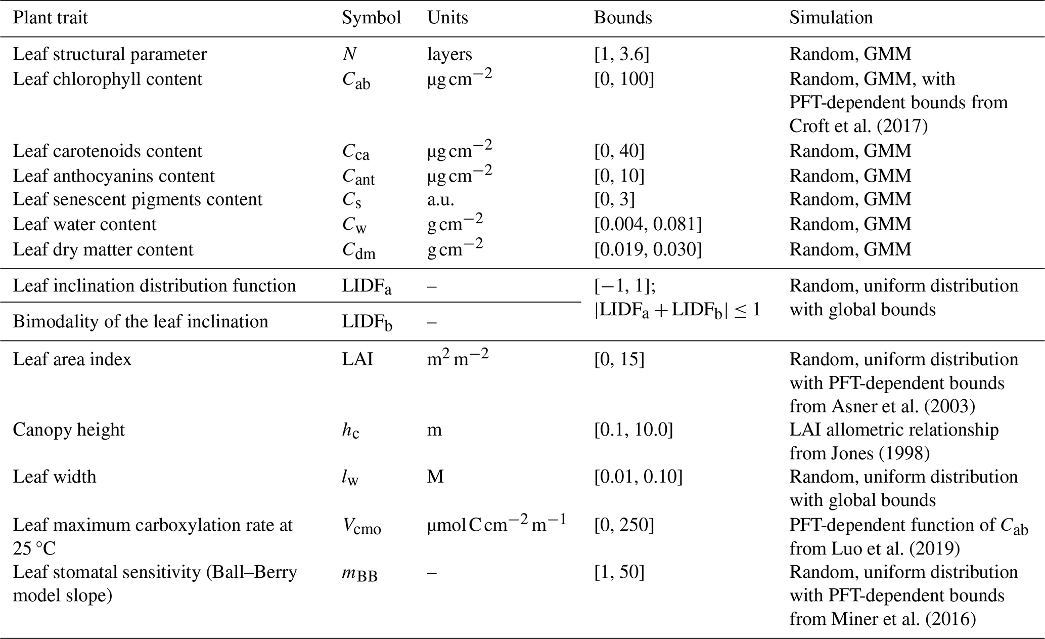
Table 1 BOSSE plant traits and variables, symbols, bounds, and the method used to produce them in the simulations.

2.2.3 Plant traits and random generator

BOSSE randomly generates sets of plant traits (i.e., radiative transfer model variables) for each pixel of a Scene, each representing a species individual or group of identical individuals. This can be constrained by PFT-dependent bounds or consider empirical relationships between traits (Table 1). BOSSE preserves the covariance between most foliar traits by drawing them from a Gaussian Mixture Model (GMM) trained over a 16 703 samples database generated by combining and gap-filling different spectral libraries and the TRY database (Kattge et al., 202) (S3 in the Supplement). The maximum carboxylation at optimal temperature (V_cmo) rate is then predicted as a PFT-dependent function of chlorophyll content (C_ab). Most structural parameters are sampled from uniform distributions within global or PFT-dependent bounds. Canopy height (h_c) is derived as a function of leaf area index (LAI).

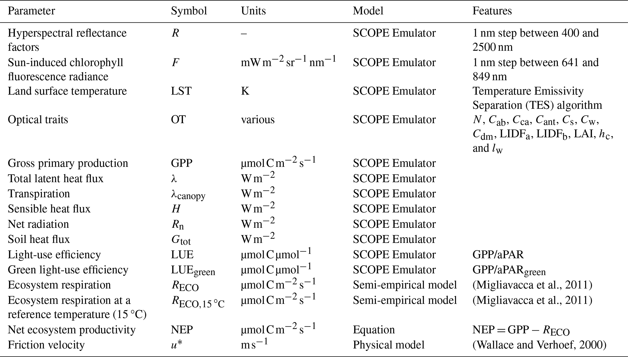
Table 2 BOSSE remote sensing products and ecosystem functions variables.

2.2.4 Remote sensing and ecosystem functions emulators

For computational feasibility, BOSSE uses emulators (i.e., 2-hidden layer neural networks; Gómez-Dans et al., 2016) of SCOPE model (Van Der Tol et al., 2009) to simulate RS imagery and most of the ecosystem functions (Table 2). The emulators predict hyperspectral R, hyperspectral F, and LST imagery as a function of plant traits, soil properties, meteorological data, and sun-view geometry (S4–S6 in the Supplement). Additional emulators retrieve optical traits (RS-based estimates of plant traits) from sun angles and R, which can also be tailored to specific RS missions (i.e., EnMAP, DESIS, and Sentinel-2 MSI) by convolving first R to their spectral response functions. An additional emulator predicts gross primary production, evapotranspiration, transpiration, sensible heat and soil heat fluxes, net radiation, and total and green light-use efficiency; ecosystem respiration is approximated with the semi-empirical model of Migliavacca et al. (2011) and used to compute net ecosystem productivity. Additionally, BOSSE computes friction velocity for the later computation of ecosystem functional properties (Gomarasca et al., 2024)

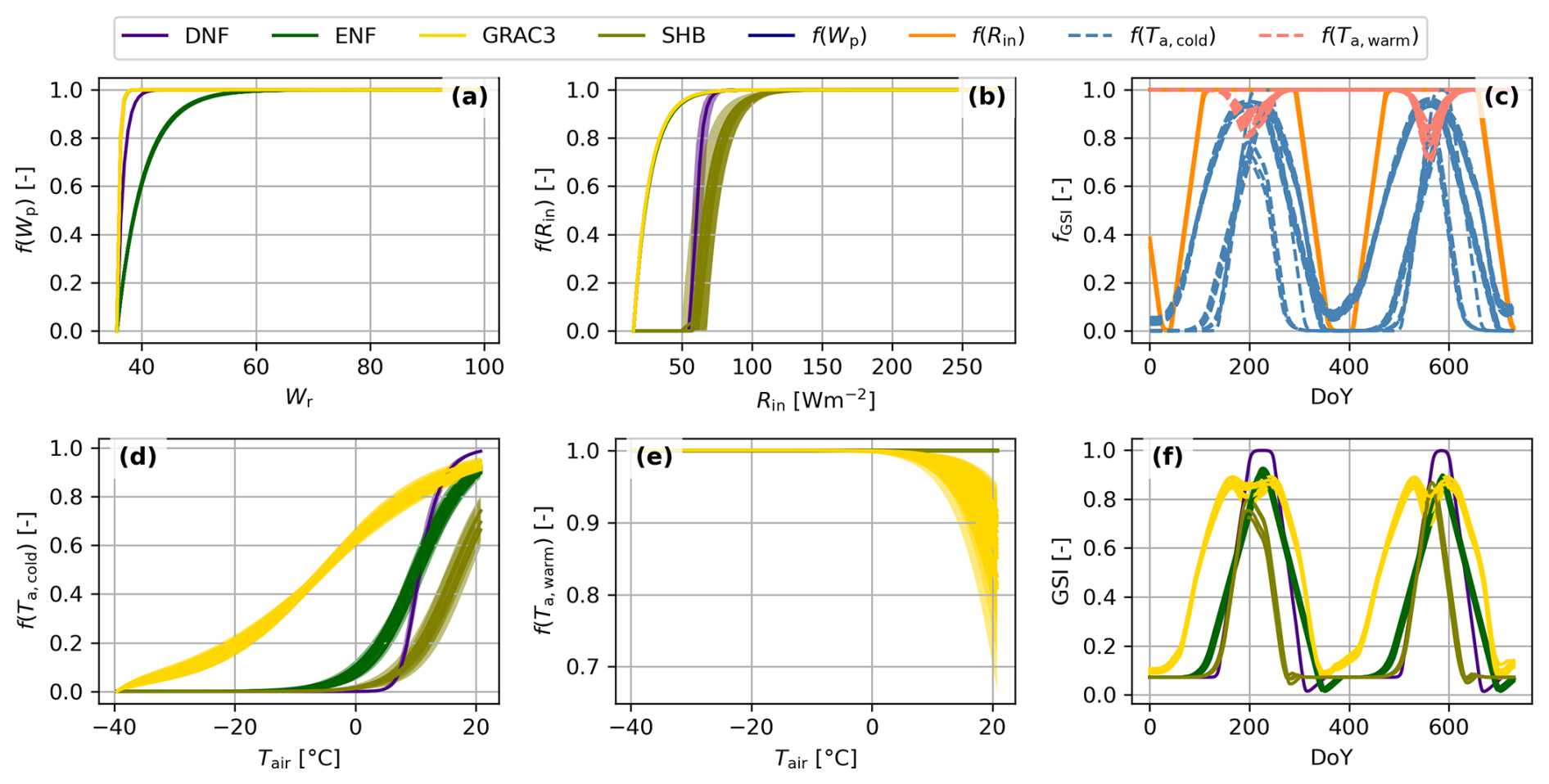
Figure 2 Components and functioning of the Growing Season Index (GSI) phenological model. Individual species response to water availability (f(W_p), a), incoming radiation (f(R_in), b), cold temperatures (f(T_a,cold), d), and warm temperatures (f(T_a,warm), e) colored by plant functional type (DNF: Deciduous Needleleaf Forest, ENF: Evergreen Needleleaf Forest, GRAC3: C3 grasslands or SHR: Shrubland) Individual species responses computed on a meteorological data time series colored by driver (c), and the GSI resulting of their product (f).

The emulators were trained over a database of simulations generated with SCOPE 1.74 using the full model (including the energy balance and photosynthesis) to ensure that spectral variables were linked to the simulated plant physiology. Vegetation traits were randomly generated (1) using a GMM trained over a plant trait database (Sect. 2.2.3) and (2) using a Latin Hypercube Sampling approach. Moreover, we developed a semi-parametric model (a 2D interpolator) predicting soil resistance for evaporation from the pore space as a function of the relative soil moisture (W_r, the ratio volumetric soil water content (SM_p) to soil field capacity (θ_fc)) and a parameter determining the sensitivity of the response (S5 in the Supplement). Realistic meteorological conditions were randomly drawn from an additional GMM trained over a 10⁵-size dataset subsampled from the BOSSE meteorological dataset (Sect. 2.2.1).

We did not only test the performance of the RS emulators to predict different RS variables on independent datasets but also assessed the impact of these uncertainties on the derived functional diversity metrics (Table S4 in the Supplement). These analyses suggested the emulator's predictions align with the expected uncertainties of the different RS products and that the fact of using emulators does not bias or jeopardize the computation of functional diversity metrics. Similarly, the emulators' capability in predicting ecosystem functions was within the uncertainties expected from eddy covariance measurements (Table S5 in the Supplement). While the emulators carry certain epistemic uncertainty, the underlying models also carry such uncertainty. As the models, the emulators establish sufficiently formal relationships between the plant traits and the RS variables used to estimate functional diversity metrics and the fluxes used to compute ecosystem functional properties, thus enabling the benchmark of methods exploring the relationships between those variables. BOSSE also allows adding random uncertainty to the simulated RS variables to match specific Gaussian noise levels.

2.2.5 Phenological model

BOSSE uses the Growing Season Index (GSI) phenological model (Forkel et al., 2014) that defines vegetation phenology as a function of its response to water availability (Fig. 2a), light (i.e., incoming shortwave radiation, Fig. 2b), as well as cold (Fig. 2d) and heat (Fig. 2e), determined by air temperature. The combination of these functions over local meteorology (Fig. 2c) leads to the combined response of each species (Fig. 2f). GSI predicts vegetation trait values at any time as a function of the boundaries assigned to each pixel and meteorology (S7 in the Supplement). BOSSE assigns the PFT-dependent values parametrized by Forkel et al. (2014) and adds random Gaussian noise to generate variability between species and between traits. The GSI runs over the 30 d averaged meteorological values, and the rate of change of the GSI index is limited for each PFT to avoid unrealistic sudden changes in the vegetation state.

Table 3 BOSSE configuration arguments.

2.3 BOSSE initialization

2.3.1 BOSSE class initialization

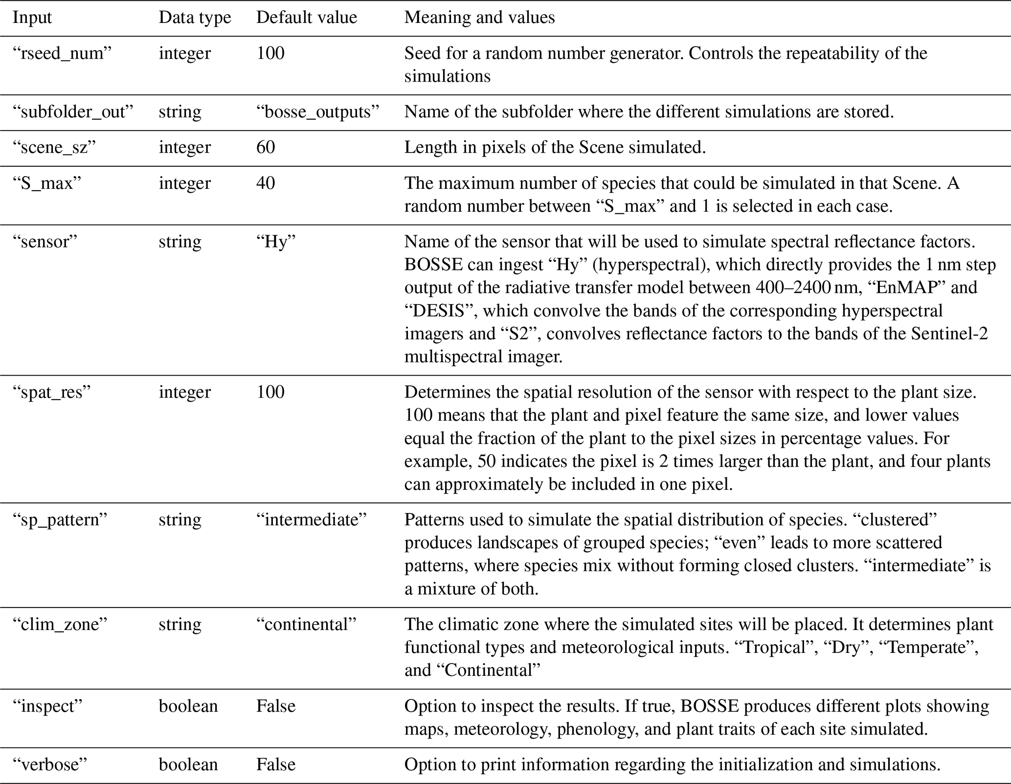
The BOSSE class is initialized by passing two Python dictionaries containing the simulation options (Table 3) and paths necessary to load all the models and constants required and to store the outputs.

During the initialization, BOSSE loads all the necessary datasets and models and preallocates 3D matrices representing the 2D Scene with the third dimension containing predefined values for all the plant, soil, and meteorological variables the model uses. BOSSE also establishes upper and lower bounds for each variable.

First, BOSSE sets the PFT-dependent information regarding:

1. The PFT and relative abundances corresponding to the selected climatic zone

2. The coefficients of the linear models relating V_cmo with C_ab from Luo et al. (2019) controlling photosynthesis and, therefore, fluorescence emission.

3. The Ball–Berry model slope (m_BB) ranges from Miner et al. (2016), controlling the ratio between photosynthesis and transpiration and, therefore, surface temperature.

4. Potential canopy conductance from Leuning et al. (2008).

5. PFT maximum leaf area index values from Asner et al. (2003).

6. Parameters of the GSI phenological model from Forkel et al. (2014): which determine phenology and are used to filter the least adapted PFTs to local meteorology.

7. The ecosystem respiration model parameters and standard error from Migliavacca et al. (2011).

Next, it loads the following models:

1. The GMM used to draw random samples of correlated plant traits.

2. SCOPE model emulators to predict spectral signals (reflectance factors, fluorescence radiance, and land surface temperature), retrieve optical traits from canopy reflectance factors of different sensors, and predict ecosystem functions.

3. The model (a 2D interpolator) predicts soil resistance for evaporation from the pore space as a function of the W_r and a parameter determining the sensitivity of the response.

2.3.2 BOSSE Scene initialization

Once BOSSE has loaded all the necessary variables and models, it can initialize a given Scene, which is controlled by the options provided when the BOSSE class is initialized (Table 3). The only necessary input argument is an integer number that identifies the meteorological dataset to be loaded. This number is used by default to seed the BOSSE class random number generators to ensure reproducibility; alternatively, the user can provide a different seed number and a low bound for the maximum mean LAI simulated in the Scene. By default, it is larger than or equal to 1.0 m² m⁻² to generate Scenes with a certain amount of vegetation. However, this value can be lowered to represent barely vegetated Scenes. The random number generator is seeded several times during the Scene initialization to maximize the comparability of the species' plant traits for the scenes generated with different spatial patterns.

Meteorological and leaf area index data

First, the time series of ERA5-Land meteorological variables are loaded for the site. Units are converted to those of the SCOPE model when necessary. Since ERA5-Land timestamps are UTC, the first and the last day might be incomplete in local time; therefore, these are gap-filled data from the nearby day, so they feature 24 hourly values at local time, which is the time used by BOSSE. Next, unfeasible negative values are interpolated and, if persistent, truncated. W_r, vapor pressure deficit, and timestamps in different formats (e.g., Day of the Year) are then computed. Finally, BOSSE calculates daily and 30 d averages and midday values and stores them in separate data frames; also, daily potential evapotranspiration is calculated using the Python package “pypyet” (Vremec et al., 2023) according to Penman-Monteith (1965).

Soil properties and climatic PFT filtering

The random number generator is seeded for the first time. Then, BOSSE randomly generates unique values of the SCOPE soil reflectance model parameters and field capacity (θ_fc, –) for the Scene. θ_fc is set within 100 %–150 % of the maximum volumetric moisture content (SM_p, %] of the time series, and water availability (W_p, –) is updated according to the new θ_fc.

Next, BOSSE uses the default PFT-dependent parameters of the phenological model and W_p to calculate the GSI time series of each PFT, utilizing the default coefficient values from Forkel et al. (2014). BOSSE filters out the PFTs that are poorly adapted to the Scene's climate. To do so, it compares the percentile 95 (or 5 for the warm temperature) of each meteorological variable with the corresponding GSI “base” parameter that determines the inflection point of the phenological response function to meteorology (see S7 in the Supplement). BOSSE removes the PFTs from the Scene where the most extreme meteorological conditions do not cross this point, assuming these are too stressful for such species to develop in competition with other species. If no PFT meets these criteria, BOSSE keeps only the most competitive PFT (reaching the largest phenological index values).

Species location and correlation with soil properties

Then, some or all of the remaining PFTs are randomly selected for the Scene, and individuals of different species are assigned to the scene pixels. BOSSE runs at a 100 % spatial resolution; therefore, each pixel is occupied by a single phenotype (a single individual or identical individuals of the same species), meaning a unique set of vegetation parameters. The number of species is randomly sampled from the range between 1 and the input “S_max” (maximum species richness). BOSSE assigns these species to the PFTs and, together with foreseen relative abundances and the spatial pattern configured (“clustered”, “intermediate”, or “even”), the Neutral Landscape model (Etherington et al., 2015) distributes them in space. Neutral Landscape produces spatial patterns of a continuous variable that is then classified to determine the pixels belonging to each species, trying to respect the foreseen abundances, which must be recomputed later. BOSSE filters this spatial pattern generated using a Gaussian kernel of standard deviation randomly selected between [0.5, 1.5] pixels. This smoothed map is then used to scale the soil reflectance model variables (B, lat, and lon), generating a spatial variability of soil properties that is partly correlated with the species' location.

Species functional traits

Plant trait values are randomly generated, either using the GMM for the leaf radiative transfer variables (N, C_ab, C_ar, C_ant, C_s, C_w, C_dm) truncated within PFT or species-dependent bounds (S3 in the Supplement) or randomly sampling within those bounds (LIDF_a, LIDF_b, LAI, l_w, and m_BB) (Table 1). Moreover, V_cmo is computed as a function of C_ab using PFT-dependent relationships from Luo et al. (2019), and canopy height (h_c) is computed using the allometric relationship with LAI and PFT-dependent scaling factors described in Jones (1998).

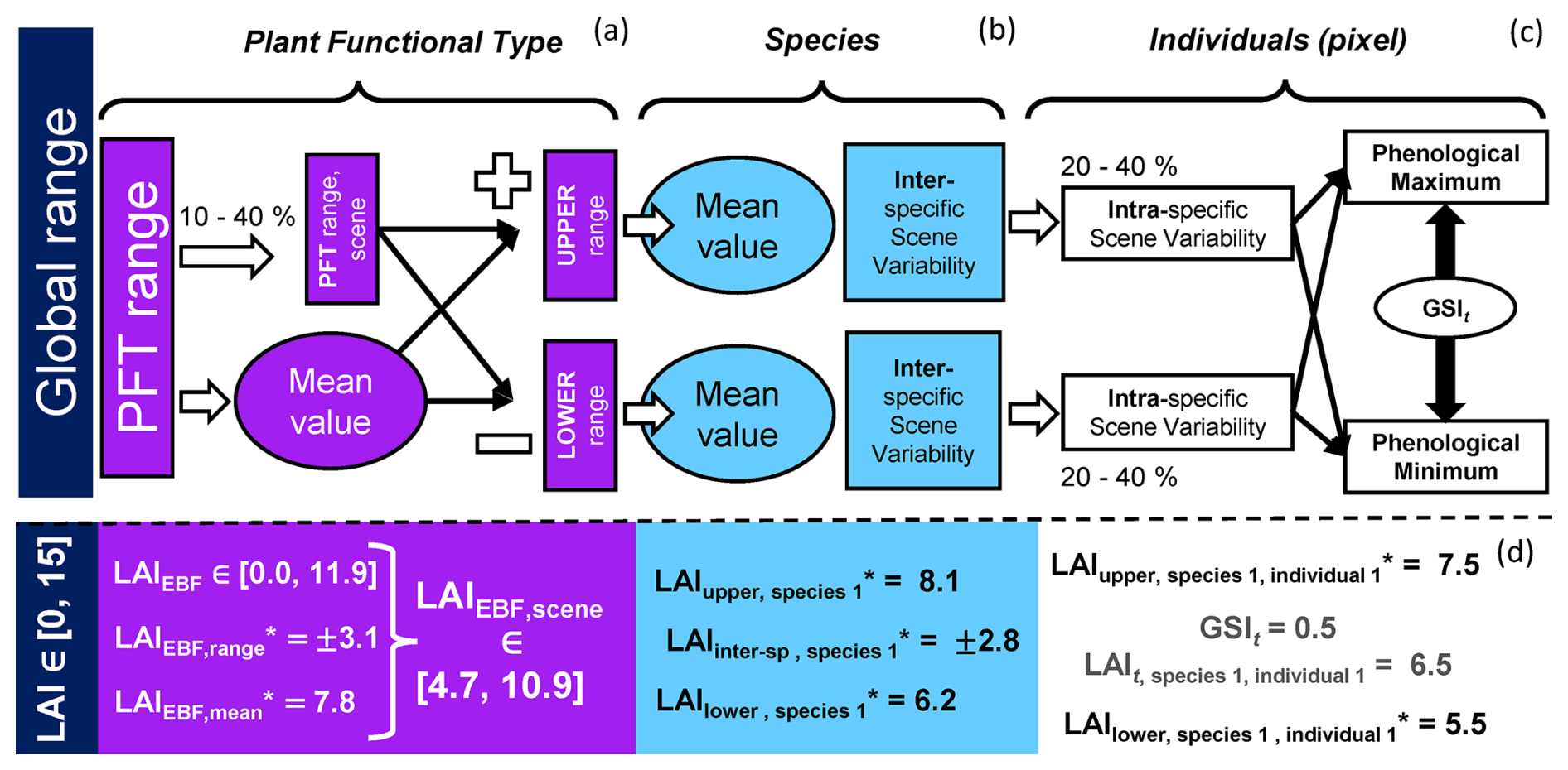
Figure 3 Generation of phenological maximum and minimum plant trait values for each plant individual (pixel). From the global or plant functional type-dependent upper and lower bounds, new bounds are set for each PFT in the scene (a), and from those, bounds are generated for each species (b), and then for each individual (i.e., pixel) including a certain intra-specific variability (c). The growing season index (GSI), ranging between [0, 1], determines the value of the traits of each individual at time t. The process is exemplified for the leaf area index (LAI) of an Evergreen Broadleaf Forest individual (EBF), where the asterisk means that the values have been randomly set within a predefined range (d).

BOSSE determines the phenological maximum and minimum values for the plant traits per pixel, considering that the bounds of some plant traits are PFT-dependent (e.g., LAI, C_ab, and m_BB). In each scene, BOSSE randomly generates a set of plant traits and a range of variability between 10 % and 40 % of the global PFT range. The bounds above and below this “central” value are used to generate random sets of mean plant traits for the species of each PFT (Fig. 3a). Then, the interspecific variability is calculated from the weighted average of the plant traits of all the species included, and the intraspecific variability is determined assuming it ranges between 20 % and 40 % of the interspecific variability (Fig. 1 in Albert et al., 2010) (Fig. 3b). Using each initial mean species plant trait values and the intraspecific variability, the plant traits of each species individual (i.e., pixel) are randomly determined. This process can bias the resulting species' mean from the initial mean value. Also, any value outside the global bounds of the above and below-average site ranges are truncated if they exceed the global trait bounds. Finally, each pixel's phenological maximum and minimum values are produced by adequately assigning the largest or the lowest value to the maximum or minimum phenological moment (Fig. 3c). For example, pigments and structural variables maximize in the green peak (GSI = 1), but senescent pigments content (C_s) are assumed minimum during that period. Also, BOSSE ensures that LAI, C_ab, carotenoids (C_ca), and anthocyanins (C_ant) content of deciduous species equal zero at the bottom of the phenological period (GSI = 0) and reduces the range of variability of all variables for the evergreen PFTs. It also ensures that the C_s only develop after the green peak (maximum GSI of the year). At any time (t) of the simulations, the plant trait values are determined by interpolating between these phenological bounds with the corresponding phenological state determined by the GSI. When LAI = 0, plant traits are set to 0, which improves the emulators' performance. The whole process is represented for a given individual in Fig. 3d.

Functional traits temporal variability

Then, the GSI phenological model is run using 30 d averages of the meteorological variables. Starting from the PFT parameter values, different parameters are generated for each species and plant trait by adding random Gaussian noise (5 % for the slope (s_GSI) and the base (b_GSI), and 1 % for the legacy sensitivity (τ_GSI), S7 in the Supplement). This allows species of the same PFT to behave similarly but prevents all the plant traits from synchronizing precisely.

BOSSE runs GSI using the incoming shortwave radiation and air temperature from ERA-5 Land. Following Forkel et al. (2014), water availability must be calculated from the relative soil water content, a PFT-defined maximum transpiration value (Table 1 in Gerten et al., 2004), potential evapotranspiration, and a PFT-dependent potential canopy conductance value from Leuning et al. (2008).

Moreover, to prevent unrealistically fast changes in the vegetation's phenological status, BOSSE includes some PFT-dependent arbitrary limits to the rate of change of the GSI index of each of the response functions of the model (Table S6 in the Supplement). During the calculation of the GSI index, these values truncated any change of the index, taking into account the time step length of the change.

Ecosystem respiration model parameters

BOSSE uses the model described and parametrized by Migliavacca et al. (2011) to predict ecosystem respiration (R_eco) and takes the PFT-dependent parameters and their associated standard errors reported in the abovementioned manuscript (S8 in the Supplement). The model scales R_eco with the maximum seasonal leaf area index, which is determined at this point for each pixel. This is done by multiplying the maximum species-dependent GSI value assigned to LAI and the LAI upper bound assigned to each pixel.

Then, for the rest of the model parameters, BOSSE first generates the interspecific variability by random sampling parameter values of a Gaussian distribution with a mean equal to the adjusted PFT-dependent value and standard deviation equal to the reported standard error in Table 5 in Migliavacca et al. (2011). Once the model parameters are defined per species, intraspecific variability is generated by adding random noise drawn from a uniform distribution, assuming traits' intraspecific variability ranges between 20 % and 40 % of the interspecific variability (Fig. 1 in Albert et al., 2010).

2.4 BOSSE simulation

BOSSE simulations always occur at 100 % spatial resolution. However, the different plant trait maps, remote sensing imagery, and ecosystem functions can be retrieved at lower resolutions where the different signals and values are averaged with different approaches depending on the nature of the variable.

2.4.1 Trait maps

BOSSE uses the precomputed plant trait bounds and the GSI values to generate plant trait maps at any time (t) of the meteorological time series. Each species and trait GSI value (${\text{GSI}}_{\text{sp},\text{PT}}\in [\mathrm{0},\mathrm{1}]$) is used to linearly interpolate the corresponding trait value between the bounds corresponding to the upper (PT_upper) and lower (PT_lower) points of the phenology, assigned for each trait and pixel (pix) of the Scene (Eq. 1). The fact that all the necessary variables are precomputed during initialization ensures the repetition of these simulations. Plant trait map resolution is degraded using a regular grid, mimicking field sampling schemes.

$$\begin{array}{}\text{(1)}& \begin{array}{rl}{\text{PT}}_{\mathrm{t},\text{pix}}=& {\text{PT}}_{\text{lower},\text{pix}}+({\text{PT}}_{\text{upper},\text{pix}}-{\text{PT}}_{\text{lower},\text{pix}})\\ & \times {\text{GSI}}_{\mathrm{t},\text{sp},\text{PT}},\end{array}\end{array}$$

2.5 Remote sensing imagery and products

BOSSE can simulate maps of plant traits and related RS imagery and products (R, F, LST, and OT) for any sample of the meteorological dataset. The phenological state (GSI value) is determined daily, and then the meteorological conditions and sun angles are set hourly. The hyperspectral reflectance factors (R, –) are initially generated at 1 nm step, between 400 and 2400 nm. These can be convolved to the spectral response functions of different RS imagers (EnMAP, DESIS, and Sentinel-2 MSI). Fluorescence radiances (F, $\mathrm{mW}{\mathrm{m}}^{-\mathrm{2}}{\mathrm{sr}}^{-\mathrm{2}}{\mathrm{nm}}^{-\mathrm{1}}$) are also provided at 1 nm step between 641 and 849 nm, and land surface temperature (LST, K) is a single layer.

In addition, RS imagery spatial resolution can be downgraded using a Gaussian point spread function (PSF) model to more accurately mimic the spatial artifacts that can occur due to the gridding step that separates RS observations from the resulting gridded imagery (Wang et al., 2020; Duveiller et al., 2011) (S9 in the Supplement). A Gaussian PSF model is currently adopted (Eq. S4 in the Supplement), aiming at considering the PSF effects only at nadir with an isotropic assumption. BOSSE spatial resolution (r_spat) is defined as the ratio of the simulation (plant) to the pixel size; therefore, a 100 % resolution implies that each pixel contains unmixed information of a unique individual or set of identical individuals. The resolution of the plant trait maps can also be degraded since many RS-related field campaigns use plots and not species as sampling units. In this case, BOSSE uses a simpler regular grid since the RS sampling process does not need to be simulated and is closer to how field data are gridded (e.g., Hauser et al., 2021). This feature would allow assessing the effect of the RS sampling at different scales (with their respective PSF effects) to see if this “erases” our capacity to detect the underlying traits accordingly.

Finally, a different set of emulators can retrieve the vegetation traits (optical traits) from the simulated R images to include the effect of the retrieval uncertainty (noise and biases) in the analyses. This retrieval is performed with emulators trained independently from the emulators predicting R (S9 in the Supplement); moreover, these emulators have been trained for specific sets of spectral bands (i.e., hyperspectral and the missions EnMAP, DESIS, and Sentinel-2). The emulators can be applied to R with any (100 % or down-graded resolution), which also allows for assessing how the loss of spatial detail propagates to the estimated optical traits.

2.5.1 Ecosystem functions

BOSSE uses instantaneous meteorological data and vegetation and soil traits to predict instantaneous gross primary production (GPP), total latent heat flux (λE), canopy latent heat flux (λE_canopy), sensible heat flux (H), net radiation (R_n), soil heat flux (G), light use efficiency (LUE), and LUE computed with the photosynthetically active radiation absorbed by chlorophyll (LUE_green) using a SCOPE dedicated emulator. Negative GPP, LUE, and LUE_green are allowed to prevent biases in averages and ecosystem functional properties, which is acceptable since these values are present in observational datasets due to uncertainty. The analysis of the simulated fluxes might be subject to quality analysis and filtering, as the observations.

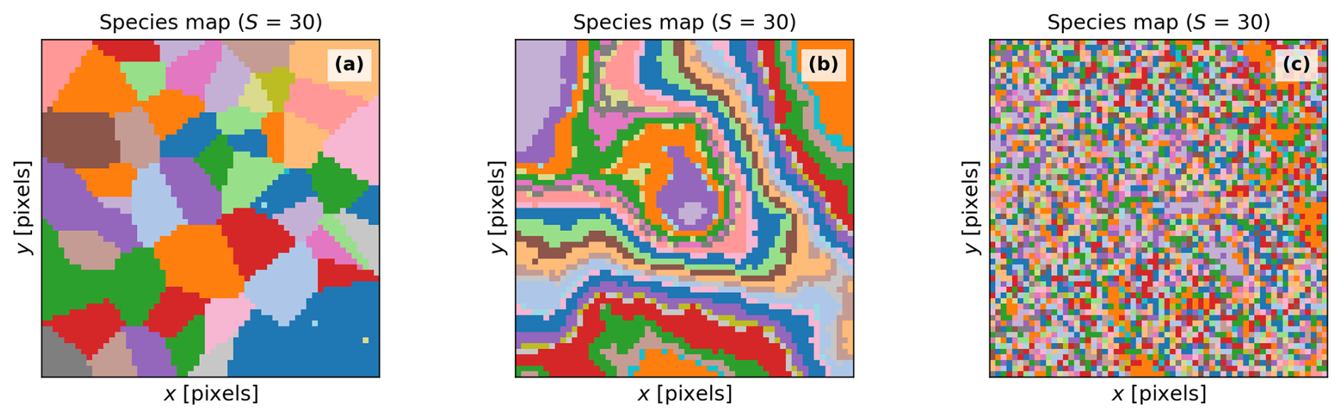
Figure 4 Simulation of a Scene with different spatial patterns: “clustered” (a), “intermediate” (b), and “even” (c). The number of species (S) is the same for all the cases; however, the relative abundance and the averaged value of the plant traits per species can vary slightly.

In addition, R_eco is computed also using the model described in Migliavacca et al. (2011). The model is parametrized to predict daily R_eco, using daily mean air temperature, daily GPP, and monthly precipitation. Therefore, the model is fed with the values averaged for those periods around the timestamp where respiration is computed. R_eco is converted to $\mathrm{\mu }\mathrm{mol}\mathrm{C}{\mathrm{m}}^{-\mathrm{2}}{\mathrm{s}}^{-\mathrm{1}}$ to calculate net ecosystem productivity (NEP = GPP−R_eco); additionally, R_eco,15 °C at the reference temperature of 15 °C is also computed. Finally, BOSSE also calculates the friction velocity (u^∗) following Wallace and Verhoef (Wallace and Verhoef, 2000), as done in the SCOPE model. The ecosystem functions can be provided as a map or as the average value for the Scene. The functions can be provided as the average value of the Scene, as well as maps so that other integration approaches (e.g., climatology footprints; Kljun et al., 2015) can be applied.

3 Results

The pyBOSSE package features a “tutorial_bosse_v1_0.ipynb” Jupyter Notebook that shows how to import the pyBOSSE and pyGNDiv packages, initialize the BOSSE class, create Scenes with different features, modify the simulations, retrieve the trait maps and the remote sensing products, visualize, store, and benchmark simulations, and compute functional diversity metrics on the maps and imagery. This section presents more advanced results (see “ManuscriptFigures.py”) that require the computation of time series in some cases, but the precomputed results are also provided.

3.1 Scene spatial patterns and species distribution

BOSSE can represent Scenes featuring the same number of species with similar plant trait values (on average) but different spatial distributions to assess its impact on the assessment of plant diversity and its relationship with ecosystem functions, if any. Figure 4a–c exemplifies the simulation of the same Scene species with three different spatial patterns: “clustered”, “intermediate”, and “even”, respectively.

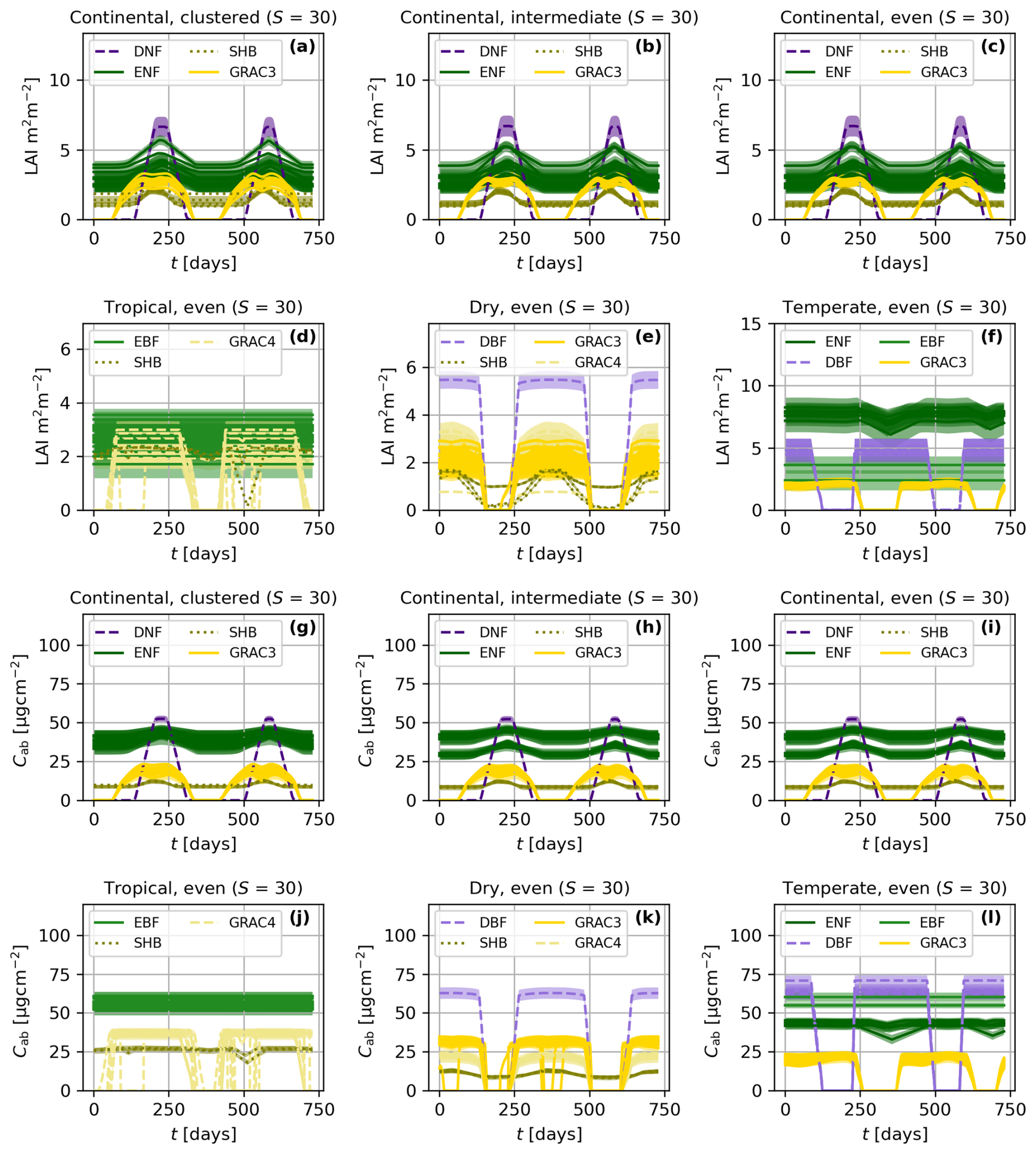
Figure 5 Time series of leaf area index (LAI, a–f) and leaf chlorophyll content (C_ab, g–l) for different spatial patterns (a–c and g–i) and climatic zones (a, d–f, g, and j–l). The averaged value of the traits and one-standard deviation (σ) confidence interval are presented per each species. The colors represent the plant functional type of each species: deciduous broadleaf forest (DBF), evergreen broadleaf forest (EBF), shrubland (SHR), C3 grassland (GRAC3), and C4 grassland (GRAC4). All the simulations feature the same species richness (S).

3.2 Vegetation phenology, intra and inter-specific variability

BOSSE simulates the time series of vegetation functional traits associated with species' individuals. Figure 5 exemplifies the simulated LAI (Fig. 5a–f) and leaf chlorophyll content (C_ab, Fig. 5g–l) for scenes in different climatic zones and spatial patterns (i.e., those in Fig. 4). Figure 5 presents the mean and one standard deviation (σ) confidence interval for each species, colored by PFTs; species richness (S) is 30 in all the cases ). For the same Scene, BOSSE ensures that the averaged values of each species are very similar across the spatial patterns (Fig. 5a–c and g–i); however, climatic conditions and local meteorology modify the PFTs and species included in each site, and therefore, their trait values (Fig. 5a, d–f, g, and j–l). The different seasonalities of evergreen and deciduous species are clearly visible and change across climates; grasses respond faster to meteorological changes than the other PFTs.

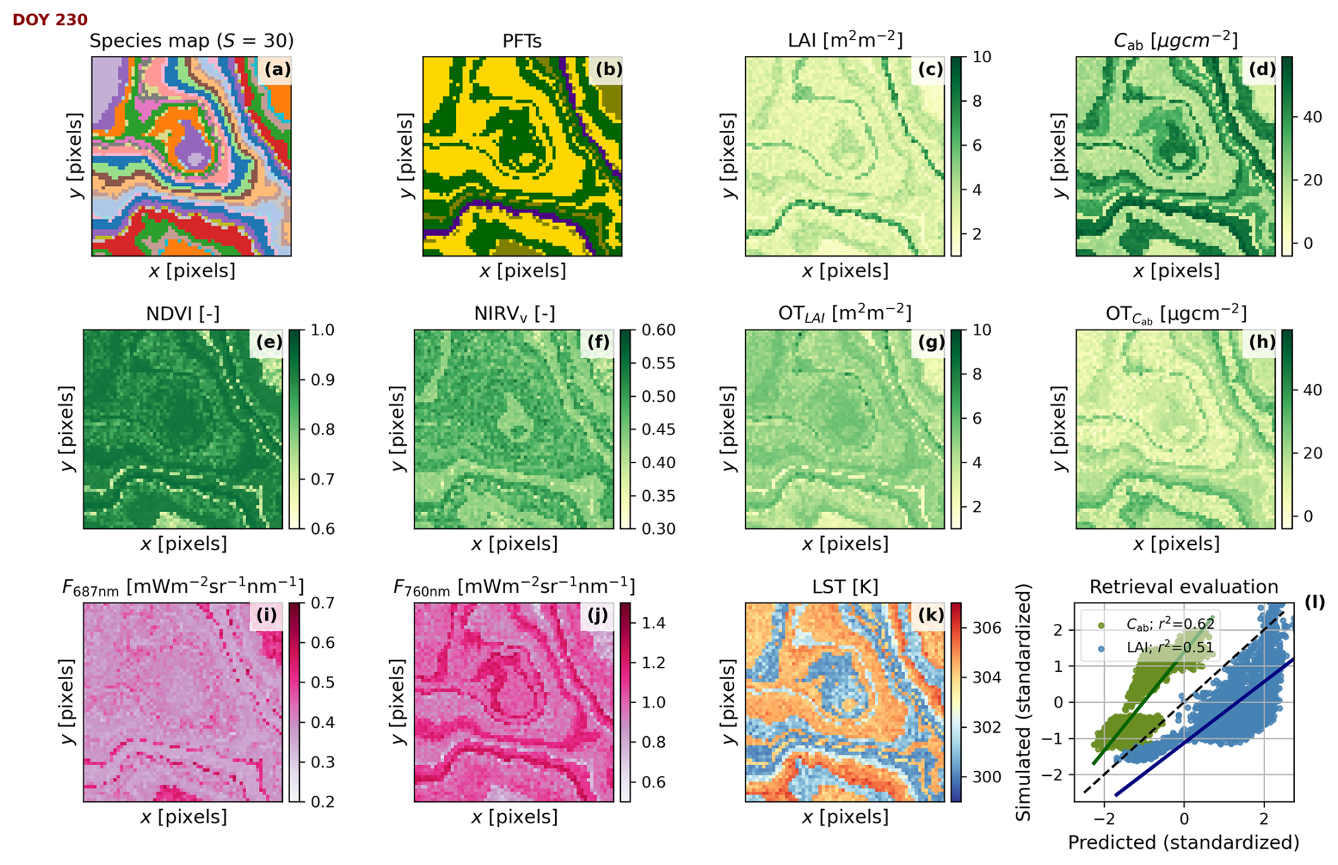
Figure 6 Simulated scene located in Continental climate and an “intermediate” spatial pattern at midday of day 230 of the time series presented in Fig. 5b and h. The coordinates are shown in pixels. Maps of species, indicating taxonomic Richness (S) (a), species' plant functional types (b), leaf area index (c), foliar chlorophyll content (d), normalized difference vegetation index (e), near-infrared reflectance of vegetation index (f), estimated leaf area index (g), estimated foliar chlorophyll content (h), fluorescence radiance at 687 nm (i), fluorescence radiance at 760 nm (j), land surface temperature (k), and the predicted vs. simulated leaf area index (c vs. g, blue) and foliar chlorophyll content (d vs. h, green)(l), standardized for the comparison and evaluated with the Pearson correlation coefficient (r²).

3.3 Scene maps, vegetation properties, and remote sensing products

Figure 6 exemplifies the simulation of Scene maps and RS products for an “intermediate” spatial pattern (see Figs. S2 and S3 in the Supplement for the “clustered” and “even” spatial pattern examples, respectively). The simulation takes place specifically at midday of day 230 of the time series presented in Fig. 5b and h, during the green peak. The species map (Fig. 6a) generated during the Scene initialization is the base to produce other maps at each timestamp. Each species is associated with a PFT (Fig. 6b). BOSSE first simulates the plant trait maps (e.g., LAI and C_ab, Fig. 5c and d) and, from those, simulates the remote sensing imagery. In this case, we computed the Normalized Difference Vegetation Index (Rouse et al., 1974) and the Near-infrared reflectance of vegetation (Badgley et al., 2017) spectral indices computed from the hyperspectral reflectance factors (Fig. 6e and f). The indices are coherent with the properties and taxonomy of vegetation. The figure also shows the fluorescence radiance at 687 and 760 nm from the hyperspectral spectra (Fig. 6i and j) and LST (Fig. 6k), which include information about the physiological status of vegetation. In addition, BOSSE can retrieve optical traits (Fig. 6g and h), each estimated with different uncertainty (Fig. 6l). In this specific case, the retrieved LAI correlates well with the simulated one. In contrast, C_ab has been overestimated and is retrieved less accurately, which is not contrasting since foliar parameters are more challenging to retrieve (e.g., Pacheco-Labrador et al., 2024). Overall, the RS images and optical traits follow the patterns presented by the vegetation traits with varying degrees of correlation. The previous relationships allow them to capture different PFD measures with various accuracy levels, alone or in combination. These correlations are the basis for assessing the capability of remote sensing to capture plant functional diversity.

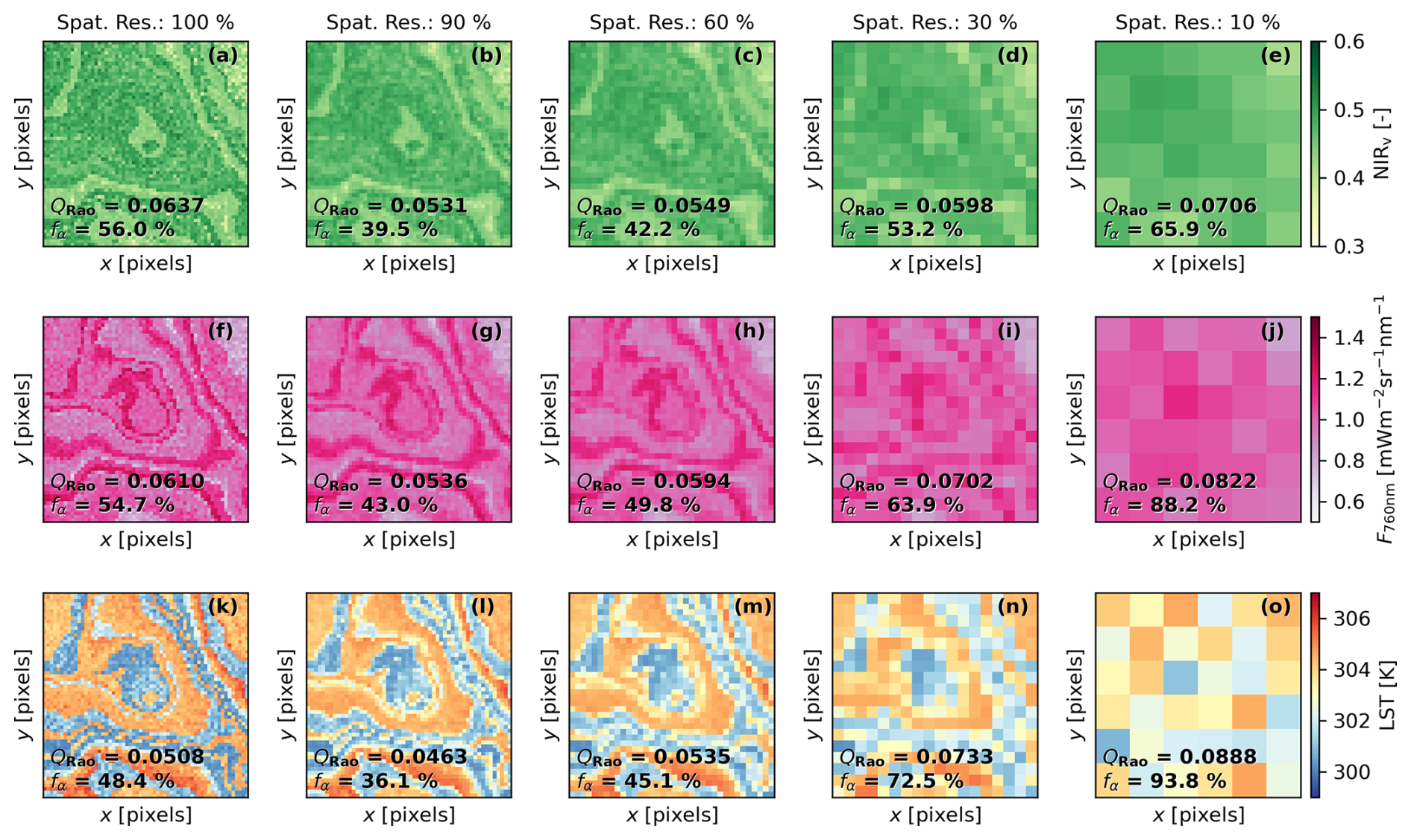
Figure 7 Simulated imagery of the near-infrared of vegetation index (a–e), fluorescence radiance at 760 nm (f–j), and land surface temperature (l–o) using an “intermediate” spatial pattern at different spatial resolutions (Spat. Res., 100 %, 90 %, 60 %, 30 %, and 10 %), defined as the plant-to-pixel size ratio. The mean value of Rao's quadratic entropy (Q_Rao) calculated over a 3 pixel × 3 pixel moving window and the fraction of α-diversity (f_α), calculated from the variance-based partition approach, are presented for each map. The coordinates are shown in pixels.

3.4 Spatial resolution and functional diversity estimates

BOSSE can simulate remote sensing imagery at different relative spatial resolutions, defined as plant-to-pixel size ratio. As the resolution coarsens, it becomes suboptimal for diversity analysis as the signals of more and more different plants are integrated into a single pixel of the coarse-resolution simulated images. This feature can help analyze suboptimal resolution estimation of PFD, enabling users to test whether a given approach is robust to a specific spatial resolution. The spatial resolution has a strong effect on the computation of the diversity metrics as shown for Q_Rao (mean of 3 × 3 windows) and f_α estimated from NIR_v (Fig. 7a–e), F at 760 nm (Fig. 7f–j), and LST (Fig. 7l–o). The loss of spatial resolution can result in both positive or negative biases according to the underlying configuration. In this case (“intermediate” spatial pattern), both metrics (Q_Rao and f_α) seem to decrease when resolution reduces to 90 % and then increase, reaching values above the ones at the 100 % resolution as it continues degrading. The behavior is also found for the other spatial patterns of the same Scene (see Figs. S4 and S5 in the Supplement for the “clustered” and “even” spatial pattern examples, respectively).

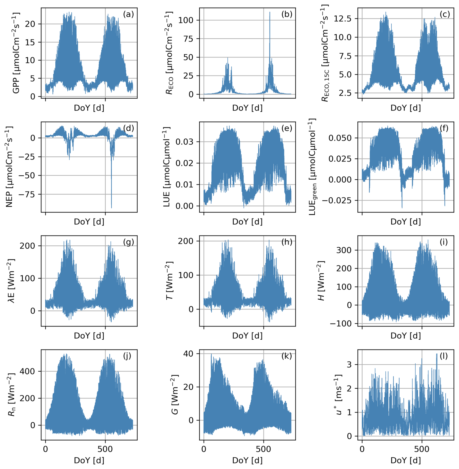
Figure 8 Time series of Scene-integrated ecosystem functions corresponding to a Scene simulated in a Continental climatic zone with an “intermediate” pattern: gross primary production (GPP, a), ecosystem respiration (R_ECO, b), ecosystem respiration at 15 °C (R_ECO,15 °C, c), net ecosystem productivity (NEP, d), light use efficiency (LUE, e), green light use efficiency (LUE_green, f), latent heat flux (λE, g), transpiration (T, h), sensible heat fluxes (H, i), net radiation (R_n, j), soil heat fluxes (G, k), and friction velocity (u^∗, l).

3.5 Ecosystem function time series

BOSSE can compute different ecosystem functions at hourly timestamps. Figure 8 shows the integrated functions corresponding to the Scene represented in Figs. 5b and 6 for 2 years. In this case, the functions are computed per pixel and averaged for the whole Scene. The fluxes follow the expected seasonal behavior, following the Scene meteorology (Fig. S6 in the Supplement), featuring one productive peak per year.

4 Discussion

BOSSE is the first Observing System Simulation Experiment (OSSE) dedicated to studying plant diversity from RS. Simulations have been recently applied to tackle methodological questions regarding the remote estimation of different aspects of plant diversity (Pacheco-Labrador et al., 2022; Pacheco-Labrador et al., 2023; Gomarasca et al., 2024; Fassnacht et al., 2022; Ludwig et al., 2024). However, none of these works have provided a sufficiently comprehensive tool to spatially describe different ecosystem types and landscapes in various climatic zones across time. Also, while simulations of all these works have explored the links between spectral and plant diversity, none of them has aimed to explore simulated BEF relationships derived from RS. BOSSE also simulates additional spectral signals beyond vegetation reflectance factors (i.e., SIF and LST), which might help elucidate these signals' potential contribution to the study of plant diversity or BEF analyses.

Despite the inherent limitations of the simulations, these are still necessary tools to clarify fundamental questions in this emerging research field. The lack of global comparable field data sets acquired for validating RS estimates of plant diversity hampers the definition and selection of reliable metrics and methodologies. This is particularly relevant for the analysis of functional diversity, where noise and uncertainty can be confounded with variability. Using simulations, Pacheco-Labrador et al. (2022) showed that some functional diversity metrics presented a large variability of performances when used at local scales (e.g., a single study site) or were prone to spuriousness under uncertainty. Therefore, the empirical results of local studies might not be sufficient to identify the most reliable methodologies, and their publication might suffer from a survivorship bias not necessarily related to the capability of approaches and metrics to capture plant functional diversity from RS. Furthermore, the SVH on which the assessment of plant diversity from remote sensing relies has been questioned (Torresani et al., 2024), and modeling and observational works have identified significant limitations (Ludwig et al., 2024; Pacheco-Labrador et al., 2022; Fassnacht et al., 2022; Wang et al., 2018). It could be that SVH is not applicable in practice or that we have not yet found reliable methodologies and the limits of their application; considering the limitations of comparable field measurements and local studies, BOSSE and similar tools might play a fundamental role in the assessment of SVH. BOSSE aims not to replace the necessary field studies but to offer a framework to answer methodological questions that improve and guide the analysis of RS imagery and validate the estimates with real-world observations.

BOSSE simultaneously simulates species and plant trait maps, the associated remote sensing signals, and the related ecosystem functions. The quality of this information can be degraded at will to test the robustness or applicability of different methodologies capturing plant diversity and BEF relationships. BOSSE relies on emulators, accepting a certain degree of epistemic uncertainty between the original model and BOSSE simulations. However, these uncertainties might not differ too much from those existing between models and reality and still offer a systematic link between the variables of interest that allows testing whether different methodologies can capture and under which circumstances. While the relationships found between BOSSE variables could not be directly transferable to real-world applications (e.g., a relationship between Q_Rao computed from R and PT), BOSSE could help to define how plant diversity or BEF relationships should be estimated (e.g., selecting the most convenient moving window sizes), and how to adapt the methodologies to different sensors (spatial resolution, spectral configuration), or observational limitations, and organize field campaigns for validation. Still, in the case of plant functional diversity, simulations have provided results close to those found with observations (e.g., Pacheco-Labrador et al., 2022). BOSSE phenology will also help to understand the role of vegetation phenological status on the reliability of diversity estimates or how to exploit this temporal information in the assessment of BEF relationships (which, so far, relies on the productive stages, e.g., Gomarasca et al., 2024).

BOSSE v1.0 offers realistic simulations but also has excellent potential to increase their complexity and completeness and tackle more challenging questions in upcoming versions. The current version already allows for testing numerous fundamental but unsolved methodological questions about how spatial resolution, phenology, and different spectral signals affect or enable the estimation of plant functional diversity. BOSSE v1.0 is already the first simulation environment providing not only reflectance factors but also other signals of interest for studying plant diversity, such as SIF (Tagliabue et al., 2020) or the less explored LST, two signals related to vegetation physiology and ecosystem functions whose role on BEF analyses remains untested. In its current state, BOSSE v1.0 might help to test and improve methodologies already developed to characterize different aspects of plant diversity (e.g., Féret and De Boissieu, 2020; Laliberté et al., 2020; Rocchini et al., 2021; Rossi and Gholizadeh, 2023, or Rossi et al., 2021), and BEF relationships (Gomarasca et al., 2024).

BOSSE relies on 1D radiative transfer models representing vertically homogeneous canopies. Future versions could rely on more complex radiative transfer models representing vertically heterogeneous canopies (e.g., SCOPE 2 (Yang et al., 2021) or DART (Gastellu-Etchegorry et al., 2017)) and simulating LiDAR datasets, which could help to develop the capability of RS to infer plant diversity in structurally complex ecosystems where different species overlap (Almeida et al., 2021; Zhao et al., 2018). Radar imagery has also been proposed as a tool to assess vegetation diversity (Bae et al., 2019; Hoffmann et al., 2022); BOSSE v1.0 could also incorporate Radar radiative transfer models (e.g., Oh and Kweon, 2013) to assess the capabilities of this signal. In its first version, BOSSE only represents nadiral observations, which limits the conclusions of the analyses in terms of missions and sun-view configurations. Future versions will include off-nadir and multi-angular capabilities to offer more realistic RS simulations of different sensors and enable the study of directional effects on the analysis of plant diversity. BOSSE will also improve the representation of vegetation and its processes. Upcoming versions will also represent plants of different sizes and include more ecological theory, allowing for the competition and replacement of species, one of the key mechanisms behind the role of plant diversity on ecosystem stability (de Bello et al., 2021). While some models already present some of the features to be included in BOSSE (e.g., FORMIND represents vegetation interactions vertically heterogeneous canopies and features a LiDAR simulator; Knapp et al., 2018), BOSSE aspires to provide more diverse features at a fast computational speed.

Beyond the study of plant diversity, BOSSE could support methodological development and benchmarking in other RS applications, particularly in those dealing with coarse spatial resolutions and integrating multiple RS products, or address scaling issues in surface-atmosphere flux modeling with low- or mid-resolution RS data. BOSSE could also support the development of digital tweens of existing landscapes via the assimilation of remote sensing and other observables.

5 Conclusions

BOSSE is the first Observing System Simulation Experiment dedicated to studying plant diversity and biodiversity–ecosystem function relationships from remote sensing. It aims to support the development of these areas, overcoming the lack of global and consistent field datasets. In its first version, BOSSE will allow researchers to test hypotheses and benchmark methodologies, while future versions will grow in complexity to help answer more nuanced and diverse research questions. BOSSE will allow researchers to select the most promising approaches, test them with real-world observations, and interpret the results by characterizing the sensitivity of the methods to different confounding factors under controlled conditions. In addition, the spatial and temporal nature of BOSSE simulations could be used for the development of other remote sensing applications. We expect BOSSE and similar modeling approaches will contribute to elucidating whether and under which circumstances the Spectral Variation Hypothesis can be reliably applied or under which circumstances.

Appendix A: Glossary

Acronym or Symbol	Definition
B	Soil brightness factor
BEF	Biodiversity-Ecosystem Function (relationships)
bGSI	Growing Season Index model sensitivity equation slope
BOSSE	Biodiversity Observing System Simulation Experiment
DBF	Deciduous Broadleaf Forest
DESIS	DLR Earth Sensing Imaging Spectrometer
EBF	Evergreen Broadleaf Forest
ECMWF	European Centre for Medium-Range Weather Forecasts
EnMAP	Environmental Mapping and Analysis Program
ERA5	ECMWF Reanalysis v5
ESA LC-CCI	European Space Agency's Land Cover Climate Change Initiative
f(Rin)	Vegetation growth response to incoming radiation
f(Ta,cold)	Vegetation growth response to cold temperatures
f(Ta,warm)	Vegetation growth response to warm temperatures
f(Wp)	Vegetation growth response to water availability
FORMIND	Forest Model Individual-Based
fα	fractions of α-diversity
fβ	fractions of β-diversity
GMM	Gaussian Mixture Model
GRAC3	C3 Grassland
GRAC4	C4 Grassland
GSI	Growing Season Index
lat	Soil “latitude” parameter (not geographical)
LiDAR	Light Detection and Ranging
lon	Soil “longitude” parameter (not geographical)
MSI	Multispectral Imager
MsTMIP	Multi-Scale Synthesis and Terrestrial Model Intercomparison Project
NACP	North American Carbon Program
OSSE	Observing System Simulation Experiment
PFD	Plant Functional Diveristy
PFT	Plant Functional Type
pix	Pixel

PSF	Point Spread Function
PT	Plant Traits
QRao	Rao's quadratic entropy index
Radar	Radio Detection and Ranging
RS	Remote Sensing
rspat	Spatial resolution
S	Species richness
SCOPE	Soil Canopy Observation, Photochemistry and Energy fluxes
sGSI	Growing Season Index model sensitivity equation slope
SHR	Shrubland
SIF	Sun-induced Chlorophyll Fluorescence
SMp	Volumetric soil water content
sp	Species
SVH	Spectral Variation Hypothesis
t	Time
TRY	Plant Trait Database
UTC	Coordinated Universal Time
Wr	Relative soil moisture
Wp	Water availability
θfc	Soil field capacity
σ	Standard deviation
τGSI	Growing Season Index model legacy sensitivity