Intercomparison of bias correction methods for precipitation of multiple GCMs across six continents

This study proposed a Comprehensive Index (CI) that jointly considers bias correction performance metrics and uncertainty to guide the selection of quantile mapping methods. This approach reveals not only a performance-based ranking of bias correction methods but also how optimal method choices shift as the uncertainty weight varies. This study evaluated daily precipitation performance from 11 CMIP6 GCMs corrected by Quantile Delta Mapping (QDM), Empirical Quantile Mapping (EQM), and Detrended Quantile Mapping (DQM) using ten evaluation metrics and applied TOPSIS (Technique for Order Preference by Similarity to an Ideal Solution) to compute performance-based rankings. Furthermore, Bayesian Model Averaging (BMA) was used to quantify both individual model and ensemble prediction uncertainties. Moreover, entropy based weighting of the ten evaluation metrics reveals that error based measures such as RMSE and MAE carry the highest information content (weights 0.13–0.28 and 0.15–0.22, respectively). By aggregating TOPSIS performance scores with BMA uncertainty measures, this study developed CI. Results show that EQM achieved the best performance across most metrics 0.30 (RMSE), 0.18 (MAE), 0.98 (R²), 0.87 (KGE), 0.93 (NSE), and 0.99 (EVS) and exhibited the lowest uncertainty (variance = 0.0027) across all continents. QDM outperformed other methods in certain regions, reaching its lowest model uncertainty (variance = 0.0025) in South America. EQM was selected most frequently under all weighting scenarios, while DQM was least chosen. In South America, DQM was preferred more often than QDM when performance was emphasized, whereas the opposite occurred when uncertainty was emphasized. These findings suggest that incorporating uncertainty leads to spatially heterogeneous and parameter dependent changes in optimal bias correction method choice that would be overlooked by metric only selection.

1 Introduction

The Coupled Model Intercomparison Project (CMIP) General Circulation Models (GCMs) have provided critical scientific evidence to explore climate change (IPCC, 2021; IPCC, 2022). Nevertheless, GCMs exhibit significant biases compared to observational data for reasons such as incomplete model parameterization and inadequate understanding of key physical processes (Evin et al., 2024; Zhang et al., 2024; Nair et al., 2023). These deficiencies with GCM have introduced various uncertainties in climate projections, making ensuring sufficient reliability in climate change impact assessments difficult. In this context, many studies have proposed various bias correction methods to reduce the discrepancies between observational data and GCM simulations, thereby providing more stable results than raw GCM-based assessments (Cannon et al., 2015; Themeßl et al., 2012; Piani et al., 2010). Despite these advancements, the suggested bias correction methods differ in their statistical approaches, resulting in discrepancies in the climate variables adjusted for historical periods. Furthermore, the distribution of precipitation across continents and specific locations causes variations in the correction outcomes depending on the method used, which makes it challenging to reflect extreme climate events in future projections and adds another layer of confusion to climate change research (Song et al., 2022b; Maraun, 2013; Ehret et al., 2012; Enayati et al., 2021). Thus, exploring multiple aspects to make reasonable selections when applying bias correction methods specific to each continent and region is necessary.

Many studies have developed appropriate bias correction methods based on various theories, which have reduced the difference between raw GCM simulations and observed precipitation (Abdelmoaty and Papalexiou, 2023; Shanmugam et al., 2024; Rahimi et al., 2021). The Quantile Mapping (QM) series has been widely adopted among bias correction methods due to its conceptual simplicity, ease of application, and adaptability to various methodologies. However, although standard QM methods have high performance in correcting stationary precipitation, they are less efficient in non-stationary data, such as extreme precipitation events (Song et al., 2022b). To address these limitations, recent studies proposed an improved QM approach to reflect future non-stationary precipitation across all quantiles of historical precipitation (Rajulapati and Papalexiou, 2023; Cannon et al., 2015; Cannon, 2018; Song et al., 2022b). In recent years, climate studies using GCMs have adopted several improved QM methods that offer higher performance than previous methods to correct historical precipitation and project it accurately into the future. For example, Song et al. (2022b) performed bias correction on daily historical precipitation over South Korea using distribution transformation methods they developed and found that the best QM method varied depending on the station. Additionally, previous studies have reported that QM performance varied by grid and station (Ishizaki et al., 2022; Chua et al., 2022). Furthermore, they compared the extreme precipitation of GCMs using the GEV distribution, which allows for more effective estimation of extreme precipitation, and demonstrated that the performance in estimating extreme precipitation varies according to different bias correction methods. From this perspective, these improved QMs may only guarantee uniform results across some grids and regions. Therefore, to analyze positive changes in future climate impact assessments, selecting appropriate bias correction methods based on a robust framework is essential.

Multi-criteria decision analysis (MCDA) is efficient for prioritization because it can aggregate diverse information from various alternatives. MCDA has been extensively used across different fields to select suitable alternatives, with numerous studies confirming its stability in priority selection (Chae et al., 2022; Chung and Kim, 2014; Song et al., 2024). Moreover, MCDA has been employed in future climate change studies to provide reasonable solutions to emerging problems, including the selection of bias correction methods for specific regions and countries (Homsi et al., 2019; Saranya and Vinish, 2021). Technique for Order Preference by Similarity to Ideal Solution (TOPSIS) is effectively utilized in our study's MCDA framework by integrating multiple evaluation metrics and calculating the distance between each alternative and the ideal solution, thereby enabling clear and intuitive prioritization decisions. However, MCDA's effectiveness is sensitive to the source and quality of alternatives, making accurate ranking challenging when information is lacking or overly focused on specific criteria (Song and Chung, 2016). Small-scale regional and observation-based studies have conducted GCM performance evaluations, but global and continental-scale evaluations are rare due to the substantial time and cost required.

GCM simulation includes uncertainties from various sources, such as model structure, initial condition, boundary condition, and parameters (Pathak et al., 2023; Cox and Stephenson, 2007; Yip et al., 2011; Woldemeskel et al., 2014). The selection of bias correction methods contributes significantly to uncertainty in climate change research using GCMs. Jobst et al. (2018) argued that GHG emission scenarios, bias correction methods, and GCMs are primary sources of uncertainty in climate change assessments across various fields. The extensive uncertainties in GCMs complicate the efficient establishment of adaptation and mitigation policies. This issue has increased awareness of the uncertainties inherent in historical simulations. Consequently, many studies have focused on estimating uncertainties using diverse methods to quantify these uncertainties (Giorgi and Mearns, 2002; Song et al., 2022a, 2023). Although it is impossible to drastically reduce the uncertainty of GCM outputs due to the unpredictable nature of climate phenomena, uncertainties in GCM simulations can be reduced using ensemble principles, such as multi-model ensemble development using a rational approach (Song et al., 2024). However, accurately identifying biases in precipitation simulation remains challenging due to the lack of comprehensive equations reflecting Earth's physical processes. In this context, climate change studies have aimed to quantify the uncertainty of historical climate variables in GCMs, offering insights into the variability of GCM simulations (Pathak et al., 2023). Bias-corrected precipitation of GCMs using QM has shown high performance in the historical period, which is expected to result in better future predictions. However, the physical concepts of various QMs may lead to more significant uncertainty in the future (Lafferty and Sriver, 2023). Therefore, efforts should be made to consider and reduce uncertainty in the GCM selection process. It will ensure the reliability of predictions by selecting an appropriate bias-correcting method. Furthermore, Bayesian Model Averaging (BMA) plays a crucial role in quantifying the predictive uncertainty of multiple climate models and enhancing the reliability of the final predictions, which is why it has been employed as an indispensable tool in our integrated evaluation.

In light of the challenges outlined above, including discrepancies among bias correction methods, regional variability in precipitation distributions, and significant uncertainties in GCM outputs, there is a clear need for an integrated framework that evaluates the performance of various QM methods and quantifies their associated uncertainties. This study aims to compare the performance of three bias correction methods using daily historical precipitation data (1980–2014) from CMIP6 GCMs across six continents (South America: SA; North America: NA; Africa: AF; Europe: EU; Asia: AS; and Oceania: OA). Ten evaluation metrics were used to assess the performance of daily precipitation corrected by the three QM methods for each continent. Subsequently, the Technique for Order of Preference by Similarity to Ideal Solution (TOPSIS) of MCDA was applied to select an appropriate bias correction method for each continent. Additionally, the uncertainty in daily precipitation for historical periods was quantified using BMA. By integrating performance scores from TOPSIS and uncertainty metrics from BMA, this study developed a Comprehensive Index (CI), which was then used to select the best bias correction method for each continent. This comprehensive approach ensures a balanced consideration of both performance and uncertainty, enhancing understanding of the bias correction process based on the distribution of daily precipitation across continents.

2 Datasets and methods

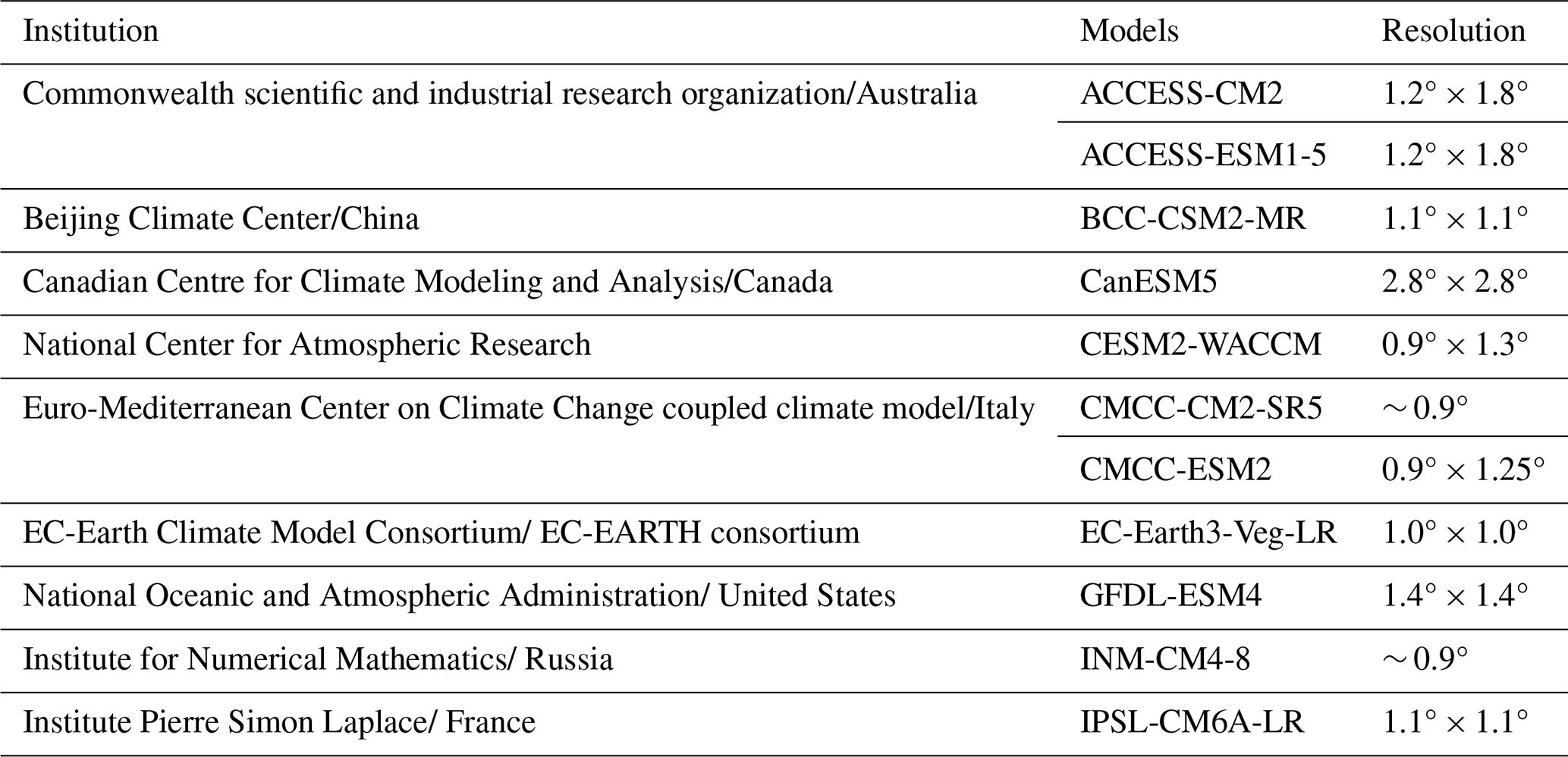
2.1 General Circulation Model

This study used 11 CMIP6 GCM to perform bias correction for daily precipitation in the historical period. The variant label for the GCMs used in this study was r1i1p1f1. Table 1 presents basic information, including model names, resolution. The model resolution of 11 CMIP6 GCMs was equally re-gridded to 1° × 1° using linear interpolation. Furthermore, this study's ensemble member of CMIP6 GCMs was the first member of realizations (r1).

Table 1 Information of CMIP6 GCMs in this study.

2.2 Reference data

This study utilized re-gridded precipitation data derived from ERA5 reanalysis products provided by the European Centre for Medium-Range Weather Forecasts (ECMWF). The original ERA5 precipitation data, available at a 0.25° × 0.25° spatial resolution, was re-gridded to a 1.0° × 1.0° resolution using the Python library xESMF. The data units were converted from meters per day (m d⁻¹) to millimeters per day (mm d⁻¹) for consistency with other datasets. The dataset is part of the FROGS (Frequent Rainfall Observations on Grids) database, which integrates various precipitation products, including satellite-based, gauge-based, and reanalysis data (Roca et al., 2019). The re-gridded dataset was selected for its spatial compatibility with the study's objectives, facilitating the evaluation of General Circulation Model (GCM) simulations in replicating observed precipitation patterns. The FROGS database provides a robust framework for intercomparison and assessment of precipitation products across different sources. FROGS database has been widely used in various studies to ensure the reliability of climate model evaluation and climate change assessment (Wood et al., 2021; Roca and Fiolleau, 2020; Petrova et al., 2024).

2.3 Quantile mapping

This study employed three (Quantile delta mapping, QDM; Detrended quantile mapping, DQM; Empirical quantile mapping, EQM) QM methods to correct the simulation of CMIP6 GCMs, and these methods are commonly used in climate change research based on the climate models (Switanek et al., 2017). The global application imposed substantial computational demands. Consequently, the scope was limited to these three techniques, and incorporating additional bias-correction methods in future work would further strengthen robustness. For calibration and evaluation, the dataset was divided into a training period (1980–1996) and a validation period (1997–2014). This approach minimizes the influence of uncertainties associated with future projections, allowing the study to focus on evaluating the intrinsic performance differences of the QM methods. The frequency-adaptation technique, as described by Themeßl et al. (2012), was applied to address potential biases and improve the accuracy of the corrections. This technique removes the systematic wet bias caused by the model's overestimation of dry days relative to observations. Based on this procedure, it effectively corrects the underestimation of excessive dry days during the summer and ensures stable performance even under rigorous cross validation. The corrected precipitation using the QM used a cumulative distribution function, as shown in Eq. (1), to reduce the difference from the reference data.

$$\begin{array}{}\text{(1)}& {\widehat{x}}_{\mathrm{m},\mathrm{p}}\left(t\right)=F_{\mathrm{o},\mathrm{h}}^{-\mathrm{1}}{F}_{\mathrm{m},\mathrm{h}}\left[x_{\mathrm{m},\mathrm{p}}\left(t\right)\right]\end{array}$$

where, ${\widehat{x}}_{\mathrm{m},\mathrm{p}}\left(t\right)$ presents the bias-corrected results. F_o,h represents the cumulative distribution function (CDF) of the observed data, and F_m,h presents the CDF of the model data. The subscripts o and m denote observed and model data, respectively, and the subscript h denotes the historical period.

QDM, developed by Cannon et al. (2015), preserves the relative changes ratio of modeled precipitation quantiles. In this context, QDM consists of bias correction terms derived from observed data and relative change terms obtained from the model. The computation process of QDM is carried out as described in Eqs. (2) to (4).

$$\begin{array}{}\text{(2)}& {\displaystyle }{\widehat{x}}_{\mathrm{m},\mathrm{p}}\left(t\right)={\widehat{x}}_{\mathrm{o}:\mathrm{m},\mathrm{h}:\mathrm{p}}\left(t\right)\cdot {\mathrm{\Delta }}_{\mathrm{m}}\left(t\right)\text{(3)}& {\displaystyle }{\widehat{x}}_{\mathrm{o}:\mathrm{m},\mathrm{h}:\mathrm{p}}\left(t\right)=F_{\mathrm{o},\mathrm{h}}^{-\mathrm{1}}\left[F_{\mathrm{m},\mathrm{p}}^{\left(t\right)}\left\{x_{\mathrm{m},\mathrm{p}}\left(t\right)\right\}\right]\text{(4)}& {\displaystyle }{\mathrm{\Delta }}_{\mathrm{m}}\left(t\right)={\displaystyle \frac{x_{\mathrm{m},\mathrm{p}}\left(t\right)}{F_{\mathrm{m},\mathrm{h}}^{-\mathrm{1}}\left[F_{\mathrm{m},\mathrm{p}}^{\left(t\right)}\left\{x_{\mathrm{m},\mathrm{p}}\left(t\right)\right\}\right]}}\end{array}$$

where, ${\widehat{x}}_{\mathrm{o}:\mathrm{m},\mathrm{h}:\mathrm{p}}\left(t\right)$ presents the bias corrected daily precipitation for the historical period, and Δ_m(t) the relative change in the model simulation between the reference period and the target period. In addition, the target period is calculated by multiplying the relative change (Δ_m(t)) at time (t) multiplied by the bias-corrected precipitation in the reference period. Δ_m(t) is defined as ${\widehat{x}}_{\mathrm{m},\mathrm{p}}\left(t\right)$ divided by $F_{\mathrm{o},\mathrm{h}}^{-\mathrm{1}}\left[F_{\mathrm{m},\mathrm{p}}^{\left(t\right)}\left\{x_{\mathrm{m},\mathrm{p}}\left(t\right)\right\}\right]$. Δ_m(t) preserving the relative change between the reference and target periods. DQM, while more limited compared to QDM, integrates additional information regarding the projection of future precipitation. Furthermore, climate change signals estimated from DQM tend to be consistent with signals from baseline climate models. The computational process of DQM is performed as shown in Eq. (5).

$$\begin{array}{}\text{(5)}& {\widehat{x}}_{\mathrm{m},\mathrm{p}}=F_{\mathrm{o},\mathrm{h}}^{-\mathrm{1}}\left\{F_{\mathrm{m},\mathrm{h}}\left[{\displaystyle \frac{{\overline{X}}_{\mathrm{m},\mathrm{h}}{X}_{\mathrm{m},\mathrm{h}}\left(t\right)}{{\overline{X}}_{\mathrm{m},\mathrm{p}}\left(t\right)}}\right]\right\}{\displaystyle \frac{{\overline{X}}_{\mathrm{m},\mathrm{p}}\left(t\right)}{{\overline{X}}_{\mathrm{m},\mathrm{h}}}}\end{array}$$

where, ${\overline{X}}_{\mathrm{m},\mathrm{h}}$ and ${\overline{X}}_{\mathrm{m},\mathrm{p}}$ represent the long-term modeled averages for the historical reference period and the target period, respectively.

EQM is a method that corrects the quantiles of the empirical cumulative distribution function from a GCM simulation based on a reference precipitation distribution using a corrected transfer function (Dequé, 2007). The calculation process of EQM can be represented as follows in Eq. (6).

$$\begin{array}{}\text{(6)}& {\widehat{x}}_{\mathrm{m},\mathrm{p}}\left(t\right)=F_{\mathrm{o},\mathrm{h}}^{-\mathrm{1}}\left(F_{\mathrm{m},\mathrm{h}}\right(x_{\mathrm{m},\mathrm{p}}\left(t\right)\left)\right)\end{array}$$

All these QMs can be applied to historical data correction in this approach. The bias correction is performed based on the relative changes between a reference period and a target period in the past, ensuring that the relative changes between these periods are preserved in the corrected data (Ansari et al., 2023; Tanimu et al., 2024; Cannon et al., 2015).

2.4 Evaluation metrics

This study evaluated the performance of three quantile-mapping methods against reference data during the validation period (1997–2014) using ten metrics commonly employed in climate research, and used these metrics to identify the optimal GCMs and bias-correction techniques. Recognizing that redundancy among metrics can bias multi-criteria decision making, this study applied an entropy-based weighting scheme that assigns weights according to each metric's distribution to enhance objectivity. Ten evaluation metrics used in this study are as follows: Root Mean Square Error (RMSE), Mean Absolute Error (MAE), Coefficient of Determination (R²), Percent bias (Pbias), Nash-Sutcliffe Efficiency (NSE), Kling-Gupta efficiency (KGE), Median Absolute Error (MdAE), Mean Squared Logarithmic Error (MSLE), Explained Variance Score (EVS), and Jenson-Shannon divergence (JSD). The equations of ten evaluation metrics are presented in Table 2.

Table 2 Information of the ten-evaluation metrics used in this study.

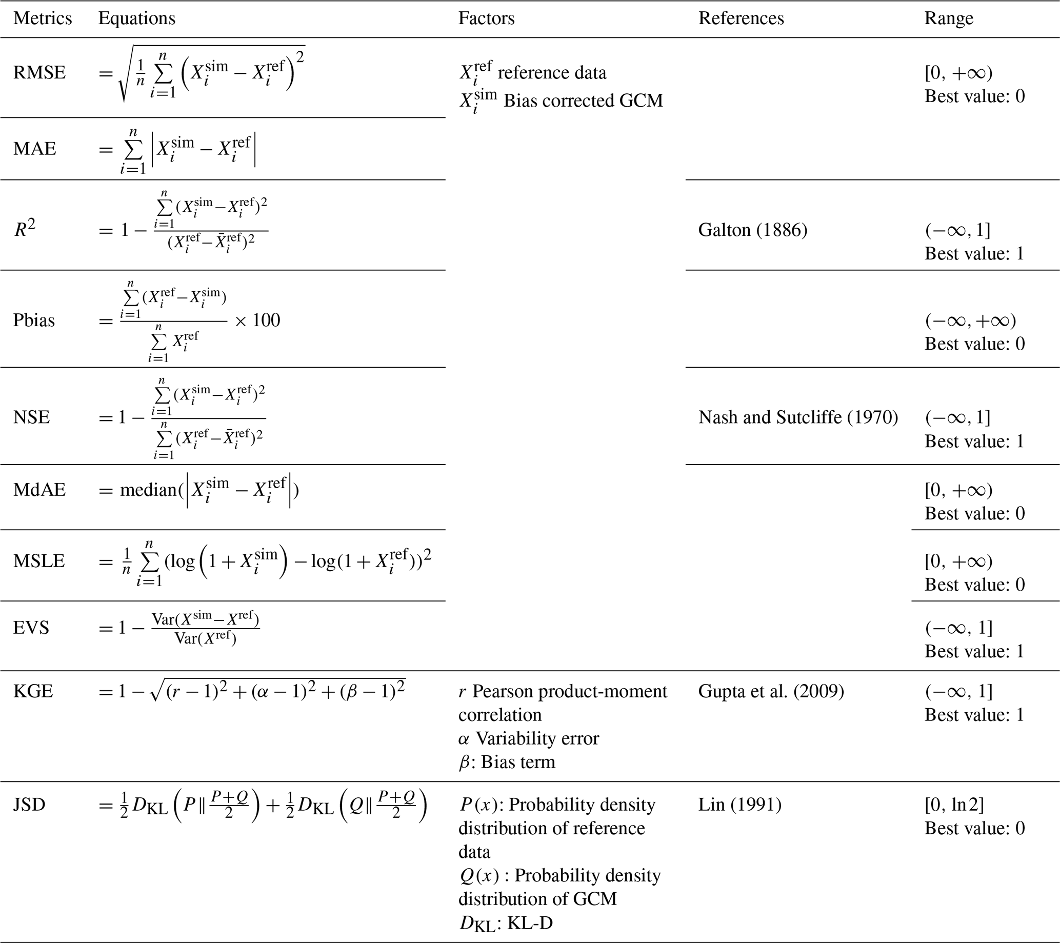
Ten evaluation metrics selected in this study assess GCM performance from various perspectives, including error (RMSE, MAE, MdAE, and MSLE), deviation (Pbias), accuracy (R², NSE), variability (EVS), correlation and overall performance (KGE), and distributional differences (JSD). These metrics complement each other by offering a comprehensive evaluation framework. For instance, while NSE evaluates the overall fit of the simulated data to observations, KGE provides a holistic view by integrating correlation, variability, and bias into a single efficiency score, and JSD captures the difference between the distributions of the reference data and the bias-corrected GCM output. This study used the Friedman test to perform statistical comparisons among the three bias-correction methods (DQM, EQM, QDM), and when the Friedman test indicated overall significant differences, pairwise Wilcoxon signed-rank tests were conducted between each method pair to determine which specific comparisons differed. The detailed concepts of the two methods can be found in Friedman (1937) and Wilcoxon (1945).

2.5 Generalized extreme value

This study used generalized extreme value (GEV) to compare the extreme precipitation calculated by the bias-corrected GCM at each grid of six continents over the historical period. The historical precipitation was compared with the distribution of reference data and bias-corrected GCM above the 95th quantile of the Probability Density Function (PDF) of the GEV distribution (Hosking et al., 1985). In addition, this study compared the distribution differences between the reference data based on the GEV distribution and the corrected GCM using JSD. GEV distribution is commonly used to confirm extreme values in climate variables. The PDF of the GEV distribution is shown in Eq. (7), and the parameters of the GEV distribution were estimated using L-moment (Hosking, 1990).

$$\begin{array}{}\text{(7)}& g\left(x\right)={\displaystyle \frac{\mathrm{1}}{s}}{\left[\mathrm{1}-k{\displaystyle \frac{x-\mathit{ϵ}}{s}}\right]}^{\frac{\mathrm{1}}{k}-\mathrm{1}}\exp \left\{-{\left[\mathrm{1}-k{\displaystyle \frac{x-\mathit{ϵ}}{s}}\right]}^{\frac{\mathrm{1}}{k}}\right\}\end{array}$$

where, k, s, and ε represents a shape, scale, and location of the GEV distribution, respectively.

2.6 Bayesian model averaging (BMA)

The BMA is a statistical technique that combines multiple models to provide predictions that account for model uncertainty (Hoeting et al., 1999). BMA is used to integrate predictions from GCMs to improve the robustness and reliability of the resulting assemblies. The posterior probability of each model is calculated based on Bayes' theorem as shown in Eq. (8).

$$\begin{array}{}\text{(8)}& P(M_k\mid D)={\displaystyle \frac{P(D\mid M_k)P\left(M_k\right)}{\sum _{j=\mathrm{1}}^{K}P(D\mid M_j)P\left(M_j\right)}}\end{array}$$

where, P(M_k) is the prior probability of model M_k, and P(D∣M_k) the likelihood of the data D given model M_k, P(M_k∣D) is the posterior probability of model M_k. In addition, the BMA prediction ${\widehat{Q}}_{\mathrm{BMA}}$ is the weighted average of the predictions from each model as shown in Eq. (9).

$$\begin{array}{}\text{(9)}& {\widehat{Q}}_{\mathrm{BMA}}=\sum _{k=\mathrm{1}}^{K}P(M_k\mid D){\widehat{Q}}_k\end{array}$$

where, ${\widehat{Q}}_k$ is the prediction from model M_k. In this study, BMA was used to quantify the model uncertainty and ensemble prediction uncertainty for daily precipitation corrected by three QM methods (QDM, EQM, and DQM) applied to 11 CMIP6 GCMs, as shown in Eqs. (10) and (11).

$$\begin{array}{}\text{(10)}& {\mathit{\alpha }}_{\mathrm{w}}^{\mathrm{2}}={\displaystyle \frac{\mathrm{1}}{K}}\sum _{k=\mathrm{1}}^K(w_k-\overline{w}{)}^{\mathrm{2}}\end{array}$$

where, K is the number of models, $w_k=P(M_k\mid D)$ is the weight of model M_k, $\overline{w}$ is the mean of the weights, given by $\overline{w}=\frac{\mathrm{1}}{K}\sum _{k=\mathrm{1}}^K{w}_k$. A higher variance in model weights indicates more significant prediction differences, implying greater model uncertainty.

$$\begin{array}{}\text{(11)}& \mathit{\sigma }\mathrm{BMA}=\sqrt{{\displaystyle \frac{\mathrm{1}}{K}}\sum _{k=\mathrm{1}}^K({\widehat{Q}}_k-\widehat{Q}\mathrm{BMA}{)}^{\mathrm{2}}}\end{array}$$

σBMA is standard deviation of the BMA ensemble predictions, ${\widehat{Q}}_k$ is the prediction from each model M_k, $\widehat{Q}\mathrm{BMA}$ is the weighted average prediction from BMA. This standard deviation represents the variability among the ensemble predictions and serves as an indicator of uncertainty. A lower standard deviation implies higher consistency among predictions, indicating lower uncertainty, while a higher standard deviation suggests greater variability and higher uncertainty.

2.7 TOPSIS

This study used TOPSIS to calculate a rational priority among three QM methods based on the outcomes derived from evaluation metrics. Moreover, this study employed entropy theory to compute objective weights for the evaluation metrics as an alternative to TOPSIS (Shannon and Weaver, 1949). The closeness coefficient calculated using TOPSIS was used as the performance metric for the CI. Proposed by Hwang and Yoon (1981), TOPSIS is a multi-criteria decision-making technique frequently used in water resources and climate change research to select alternatives (Song et al., 2024). As described in Eqs. (12) and (13), the proximity of the three QM methods is calculated based on the Positive Ideal Solution (PIS) and the Negative Ideal Solution (NIS).

$$\begin{array}{}\text{(12)}& {\displaystyle }{D}_i^{+}=\sqrt{\sum _{j=\mathrm{1}}^n{w}_j(f_j^{+}-f_{i,j}{)}^{\mathrm{2}}}\text{(13)}& {\displaystyle }{D}_i^{-}=\sqrt{\sum _{j=\mathrm{1}}^n{w}_j(f_j^{-}-f_{i,j}{)}^{\mathrm{2}}}\end{array}$$

where, $D_i^{+}$ is the Euclidean distance of each criterion from the PIS, summing the whole criteria for an alternative $f_j^{+}$, j presents the normalized value for the alternative $f_j^{+}$. w_j presents weight assigned to the criterion j. $D_i^{-}$ is the distance between the alternative $f_j^{-}$ and the NIS. The relative closeness is calculated as shown in Eq. (14). The optimal value is closer to 1 and represents a reasonable alternative.

$$\begin{array}{}\text{(14)}& C_i={\displaystyle \frac{D_i^{-}}{(D_i^{-}+D_i^{+})}}\end{array}$$

This study used entropy theory to calculate the weights for each criterion. Entropy weighting ensures sufficient objectivity by calculating weights based on the variability and distribution of data. This approach minimizes subjectivity, preventing biases in the weighting process.

2.8 Comprehensive index (CI)

This study proposed a CI to select the best QM method by combining performance scores and model uncertainty indicators. The CI integrates the performance scores (closeness coefficient) derived from the TOPSIS method with the uncertainty quantified using BMA. This approach allows for a balanced evaluation that considers both the effectiveness of the QM methods and the associated uncertainties. Uncertainty was quantified in two ways. Model-specific weight variance was calculated using the variance of the model weights assigned by BMA, representing the uncertainty in selecting the appropriate QM. The standard deviation of BMA ensemble prediction was calculated to capture the spread and, thus, the uncertainty of the ensemble forecasts. Both the indicators were normalized using a min-max scaler to ensure comparability. The CI is calculated individually for every grid and can reflect climate characteristics. Framework provides flexibility in determining the weighting of uncertainty or performance depending on the study objectives. Additionally, the methodology offers flexibility in selecting performance and uncertainty metrics. Alternative MCDA methods beyond TOPSIS can be utilized for performance indicators, or indices that effectively represent the model's performance can be employed to calculate the CI. Similarly, for uncertainty indicators, approaches such as variance, standard deviation, or other uncertainty quantification techniques can be applied to enhance the robustness of the framework further. Finally, the calculation process of the CI is performed as shown in Eqs. (15) and (16).

$$\begin{array}{}\text{(15)}& {\displaystyle }\mathrm{UI}={\displaystyle \frac{V_{\mathrm{w}}+{\mathit{\sigma }}_{\mathrm{e}}}{\mathrm{2}}}\text{(16)}& {\displaystyle }\mathrm{CI}=\mathit{\omega }\times C_i-\mathit{\beta }\times \mathrm{UI}\end{array}$$

where,UI represents the uncertainty indicator. V_w and σ_e represent the normalized weight variance and the normalized ensemble standard deviation, respectively, calculated using BMA. C_i represents the closeness coefficient calculated from TOPSIS. ω represents the weight given to the performance score, β represents the weight given to the uncertainty indicator. Furthermore, by adjusting the weights ω and β, the study evaluated the QM methods under different scenarios. Equal weight (ω=0.5, β=0.5) balances performance and uncertainty equally, and the emphasized performance weight (ω=0.7, β=0.3) prioritize performance over uncertainty. The emphasized uncertainty weight (ω=0.3, β=0.7) prioritize uncertainty over performance. The results from the CI provide a holistic evaluation of the QM methods, considering both their effectiveness in bias correction and the reliability of their predictions.

3 Result

3.1 Assessment of bias correction reproducibility across continents

3.1.1 Comparison of bias correction effects

A Taylor diagram was used to compare the bias-corrected and raw GCM precipitation with the observed data, and Fig. 1 presents the results of applying the three QM methods to 11 CMIP6 GCMs. In general, the precipitation corrected by DQM showed a larger difference from the reference data than other methods. In contrast, EQM performed better than DQM, and many models showed results close to the reference data. The precipitation corrected by QDM also showed good performance in most continents but slightly lower than EQM. Nevertheless, QDM showed clearly better results than DQM.

Regarding correlation coefficients, precipitation corrected by DQM showed relatively high values between 0.8 and 0.9 but lower than EQM and QDM. The precipitation corrected by EQM showed high agreement with the reference data, recording correlation coefficients above 0.9 in most continents. QDM generally showed similar correlation coefficients to EQM but slightly lower values than EQM in North America and Asia. For RMSE, precipitation corrected by DQM was higher than EQM and QDM, indicating that the corrected precipitation differed more from the reference data. On the other hand, EQM had the lowest RMSE and showed superior performance compared to other methods. QDM had slightly higher RMSE than EQM but still outperformed DQM.

In terms of standard deviation, precipitation corrected by DQM was higher or lower than the reference data in most continents. On the other hand, precipitation corrected by EQM was similar to the reference data and almost identical to the reference data in Africa and Asia. QDM was similar to the reference data in some continents but showed slight differences from EQM.

These results imply that the precipitation corrected by the three methods outperforms the raw simulation, which confirms that the GCM's daily precipitation is reliably corrected in the historical period.

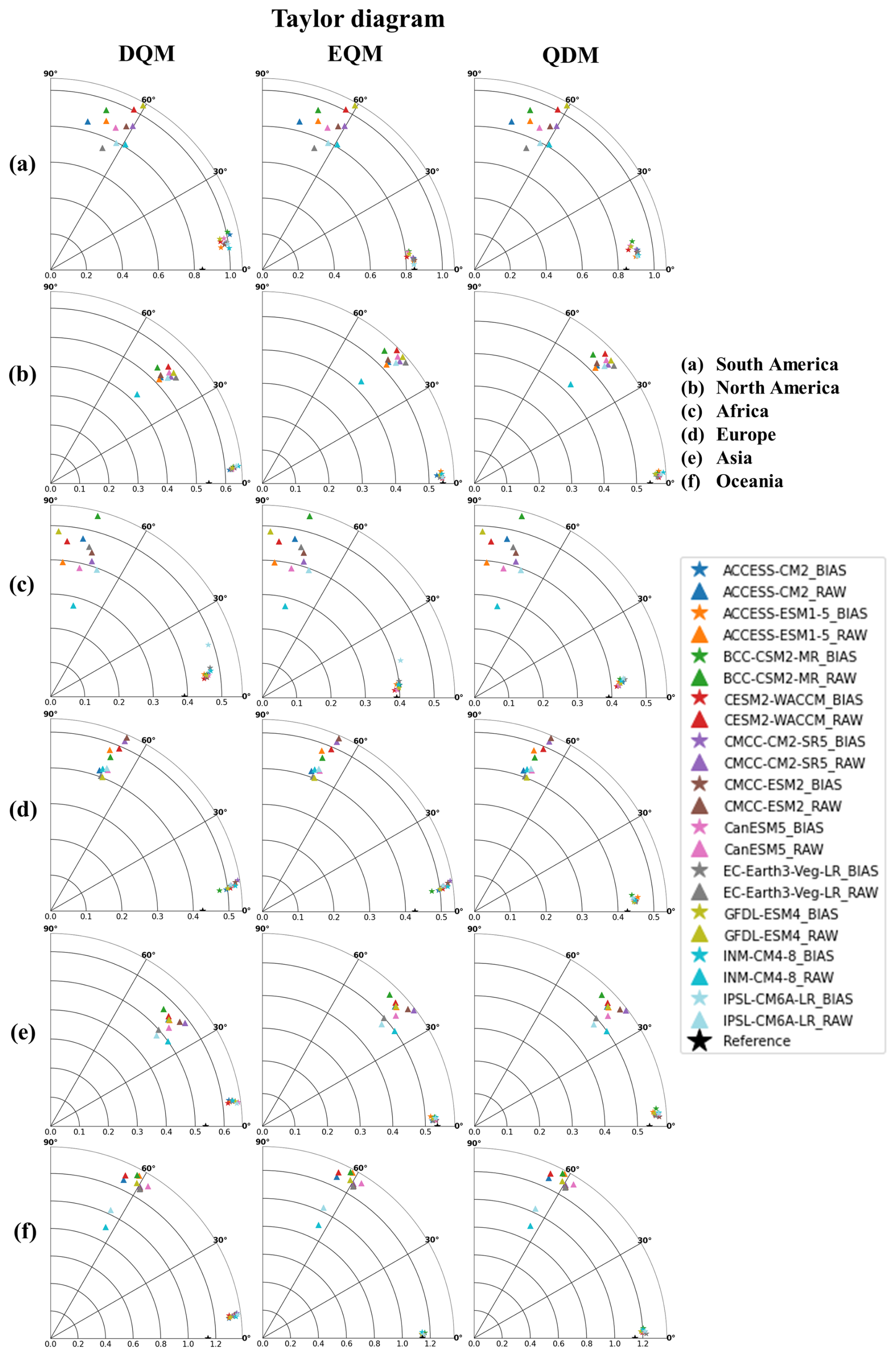
Figure 1 Comparison of raw and bias-corrected daily precipitation across six continents during the validation period (1997–2014) using Taylor diagrams (x-axis: standard deviation; y-axis: correlation coefficient).

3.1.2 Spatial distribution of bias correction performance

This study used the Friedman test to evaluate whether the three quantile-mapping methods (QDM, DQM, EQM) rank differently across the 11 downscaled GCMs for each of the ten-evaluation metrics within each continent. A p-value < 0.05 indicates that the methods rank differently for the metric, and in this section all Friedman p-values were < 0.001 (Table S1 in the Supplement). When the Friedman test was significant, pairwise differences were examined with the Wilcoxon signed-rank test. The results, summarized in Supplement Fig. S1, show that most method pairs are significant across continents.

The spatial patterns of the evaluation metrics computed from the bias-corrected daily precipitation data of GCMs in South America are presented as shown in Fig. 2. Overall, the precipitation corrected by EQM demonstrated lower JSD values, as well as higher EVS and KGE values, compared to other methods. The precipitation corrected by EQM showed higher EVS in certain regions but slightly lower performance in MdAE and Pbias across some grids. DQM exhibited performance similar to EQM and QDM in most evaluation indices but was relatively lower in most evaluation metrics. The precipitation corrected by the three methods was underestimated compared to the reference data in northern South America, while it was overestimated in eastern South America. In addition, precipitation corrected by the DQM method tended to be overestimated more than the other methods, while the EQM method showed the opposite result. Furthermore, the daily precipitation corrected by EQM showed the lowest overall error and high performance in both NSE and R². QDM and DQM also performed well but exhibited slightly larger errors in some regions than EQM.

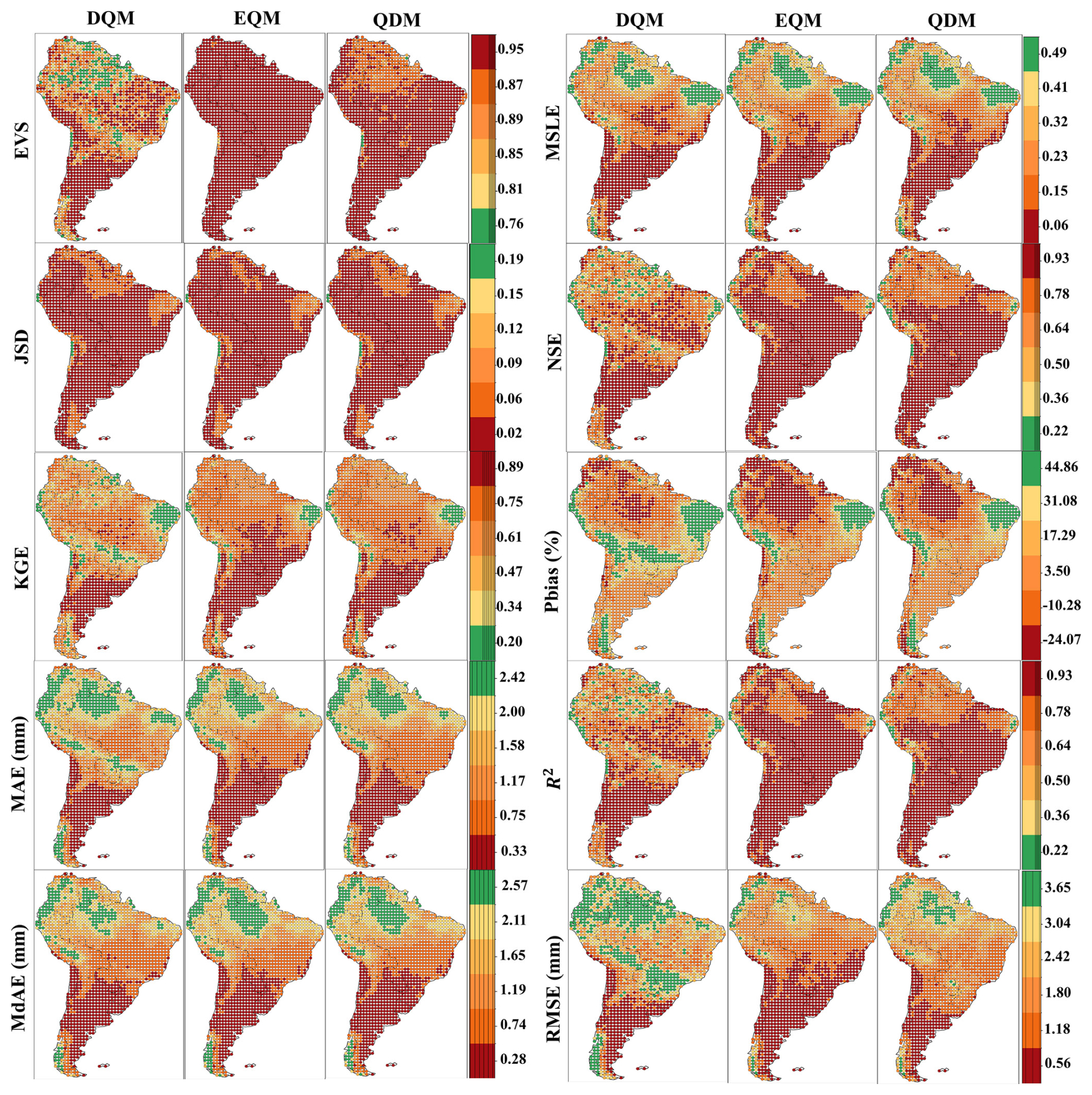
Figure 2 Performance comparison of DQM, EQM, and QDM for the validation period (1997–2014) using evaluation metrics for daily precipitation in South America.

Figure 3 shows spatial patterns of evaluation metrics for bias-corrected daily precipitation in North America. DQM exhibited poorer error performance (MAE, MSLE, RMSE, MdAE), especially in the southern region, while EQM achieved the best error metrics continent wide and QDM's errors were only slightly higher. For correlation metrics (NSE, R²), EQM yielded the highest coefficients (mostly above 0.995), DQM lagged except for some high values in central and eastern grids, and QDM showed slightly lower correlations (around 0.978). All three methods overestimated precipitation (Pbias) at most grid points, with notable underestimation in Greenland. On divergence and distribution metrics (JSD, EVS, KGE), EQM again outperformed both DQM and QDM. Consequently, EQM consistently provided the most accurate and reliable precipitation corrections in North America, while DQM introduced the greatest uncertainty.

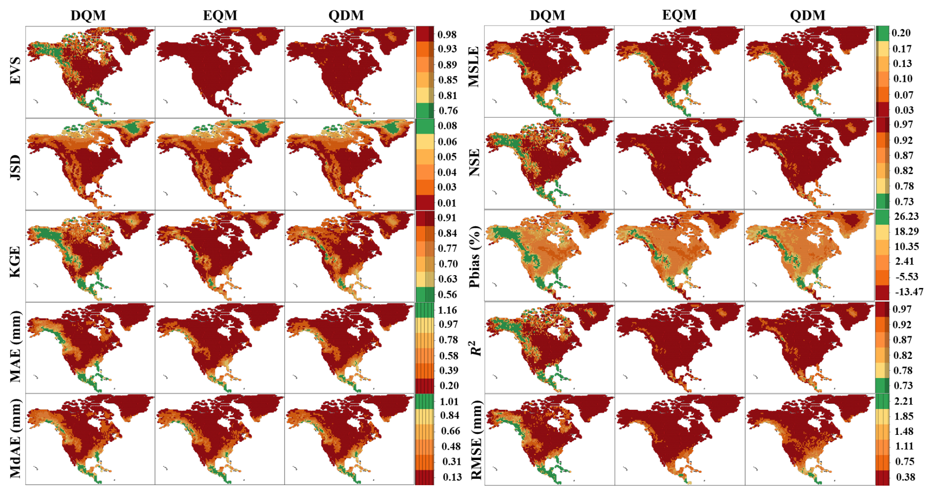
Figure 3 Performance comparison of DQM, EQM, and QDM for the validation period (1997–2014) using evaluation metrics for daily precipitation in North America.

Daily precipitation in Africa was corrected using three QM methods, and performance is shown in Fig. 4. All three methods produced similar JSD spatial patterns, though DQM's performance was notably lower in southern Africa. In terms of EVS, DQM exhibited the highest variability, QDM was intermediate, and EQM showed the lowest variability in southern and central regions (but remained high in the north). For error metrics, QDM performed best overall, particularly in North Africa (MAE = 0.03, MSLE = 0.004), followed by EQM, then DQM. EQM achieved the highest correlation scores (NSE and R²) across most grid points, with QDM outperforming DQM.

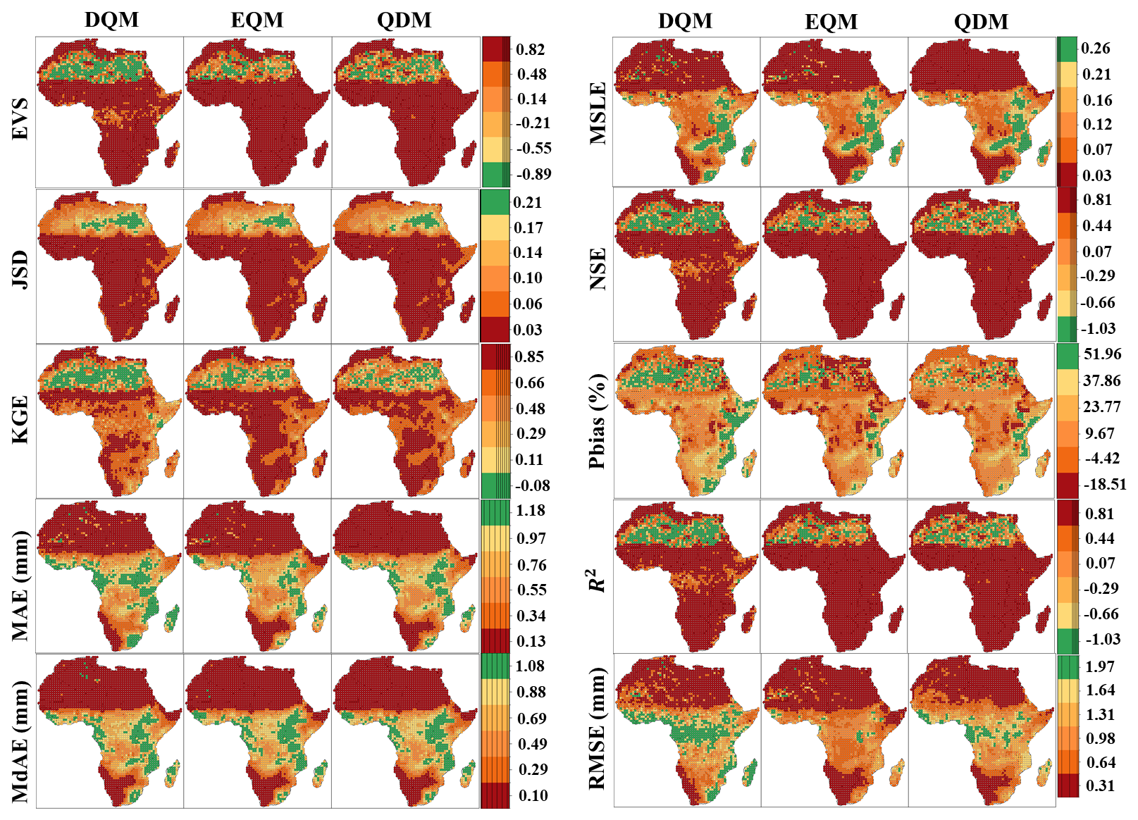
Figure 4 Performance comparison of DQM, EQM, and QDM for the validation period (1997–2014) using evaluation metrics for daily precipitation in Africa.

Figure 5 shows the spatial results of the grid-based evaluation metrics for the European region. In terms of error metrics, EQM-corrected precipitation performed the best across Europe compared to other methods. In contrast, QDM-corrected precipitation performed similarly to DQM in MAE and MSLE but significantly outperformed DQM in RMSE.

Regarding NSE and R², EVS, and KGE metrics, EQM-corrected precipitation performed overwhelmingly better than other methods. QDM precipitation performed better than DQM, while DQM performed the worst. Regarding Pbias, EQM-corrected precipitation was underestimated compared to the reference data in most parts of Europe. In contrast, QDM-corrected precipitation was more similar to the reference data compared to other methods, and DQM precipitation was overestimated compared to the reference data except in central Europe.

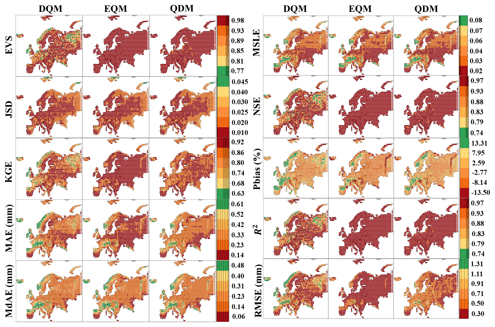
Figure 5 Performance comparison of DQM, EQM, and QDM for the validation period (1997–2014) using evaluation metrics for daily precipitation in Europe.

Figure 6 compares bias-corrected daily precipitation in Asia using various evaluation metrics. For error metrics, EQM provided the best performance its RMSE remained below 1.35 over most regions while DQM had the lowest errors. QDM's error values were similar to EQM but slightly higher in East and North Asia. In terms of NSE and R², EQM again led, especially in Southwest and East Asia, with DQM lagging behind. For EVS, EQM showed the lowest variability, QDM was intermediate, and DQM the highest. Regarding Pbias, DQM tended to overestimate precipitation continent wide, EQM underestimated in most areas except Central Asia, and QDM's spatial pattern resembled EQM but with a wider Pbias range.

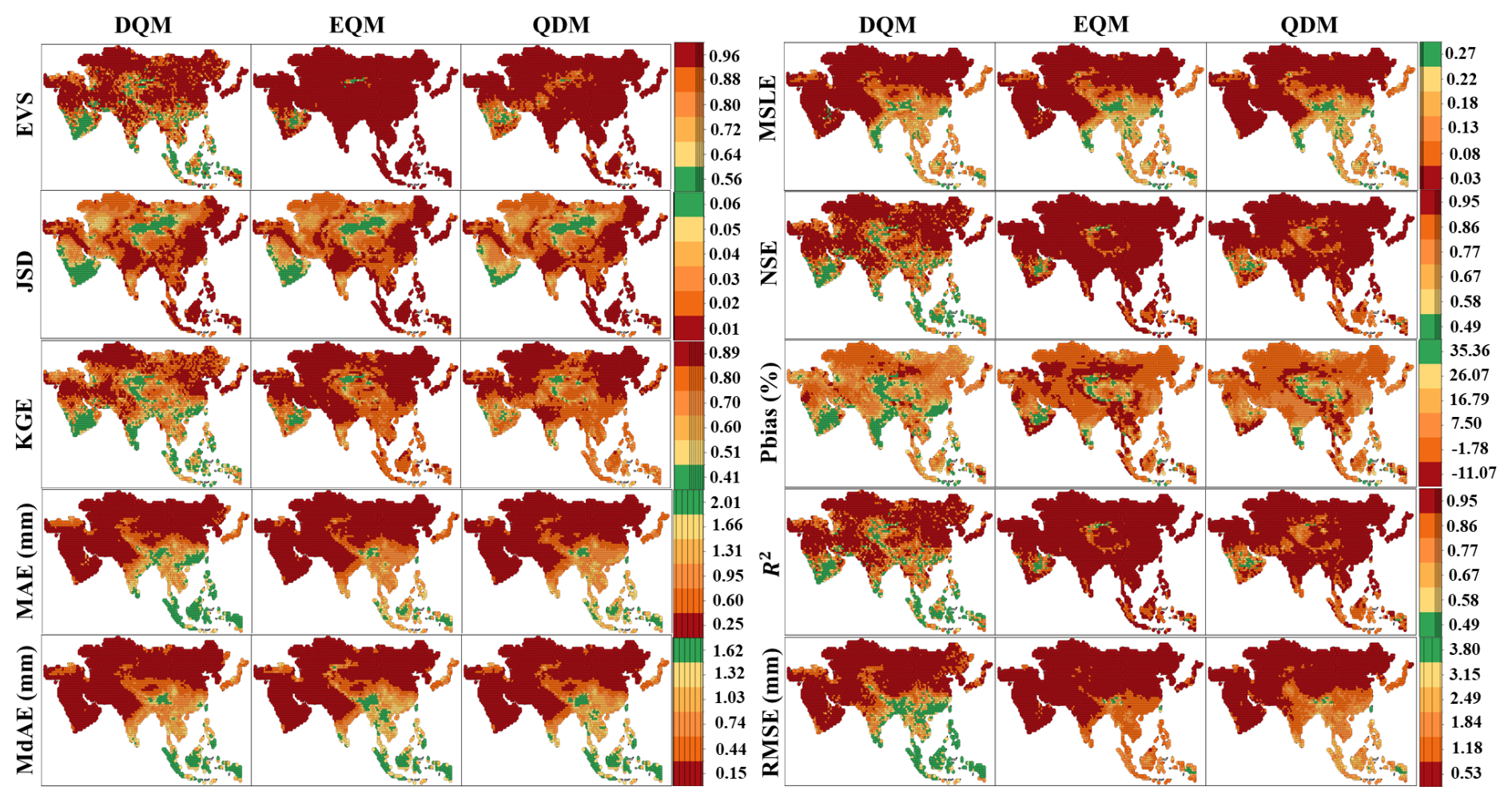
Figure 6 Performance comparison of DQM, EQM, and QDM for the validation period (1997–2014) using evaluation metrics for daily precipitation in Asia.

Figure 7 shows the results of spatially quantifying the corrected daily precipitation in Oceania using various evaluation metrics. In terms of error metrics, the precipitation estimated by the three QM methods performed similarly in MAE, MdAE, and MSLE. However, the precipitation corrected by EQM performed better in RMSE than the other methods. In the case of JSD, all three methods performed well. Regarding EVS, the precipitation corrected by EQM showed lower variability than the other methods, and DQM showed higher performance than QDM. In Pbias, the precipitation adjusted by QDM was overestimated compared to the reference data in Oceania, while the precipitation corrected by DQM and EQM was underestimated compared to the reference data in central and southern Oceania. Finally, in KGE, precipitation corrected by EQM showed the highest performance, while DQM showed the lowest.

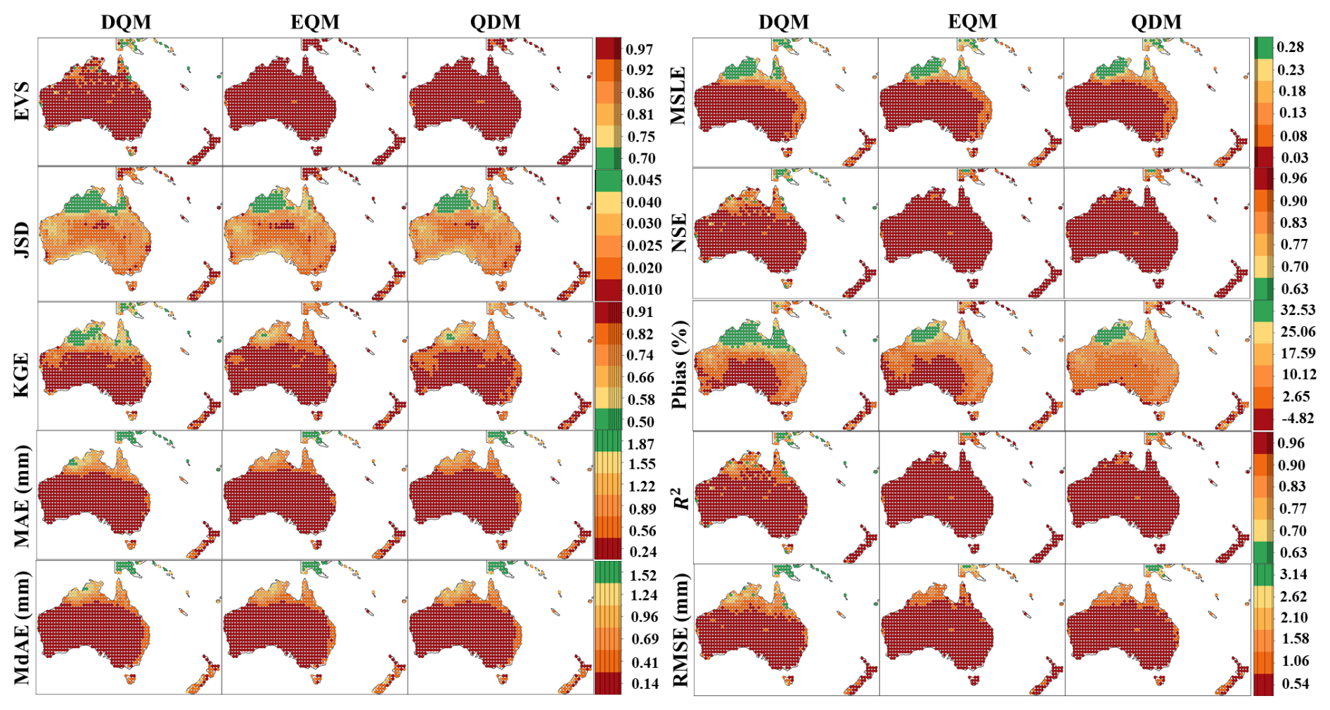
Figure 7 Performance comparison of DQM, EQM, and QDM for the validation period (1997–2014) using evaluation metrics for daily precipitation in Oceania.

Figure 8 presents the distribution of the ten-evaluation metrics for bias-corrected daily precipitation averaged over each continent, summarized as boxplots. Each box shows the interquartile range (IQR) and median of the metric values computed over 11 CMIP6 GCMs. Overall, EQM's boxes generally have lower medians and narrower IQRs for error metrics (RMSE, MSLE, MAE) on most continents, indicating both smaller typical errors and less scatter compared to QDM and DQM. QDM's boxplots lie slightly above those of EQM but still exhibit relatively tight IQRs, suggesting consistently strong performance. In contrast, DQM often has higher median errors, wider IQRs, and more extreme outliers, reflecting larger and more variable biases relative to the other methods.

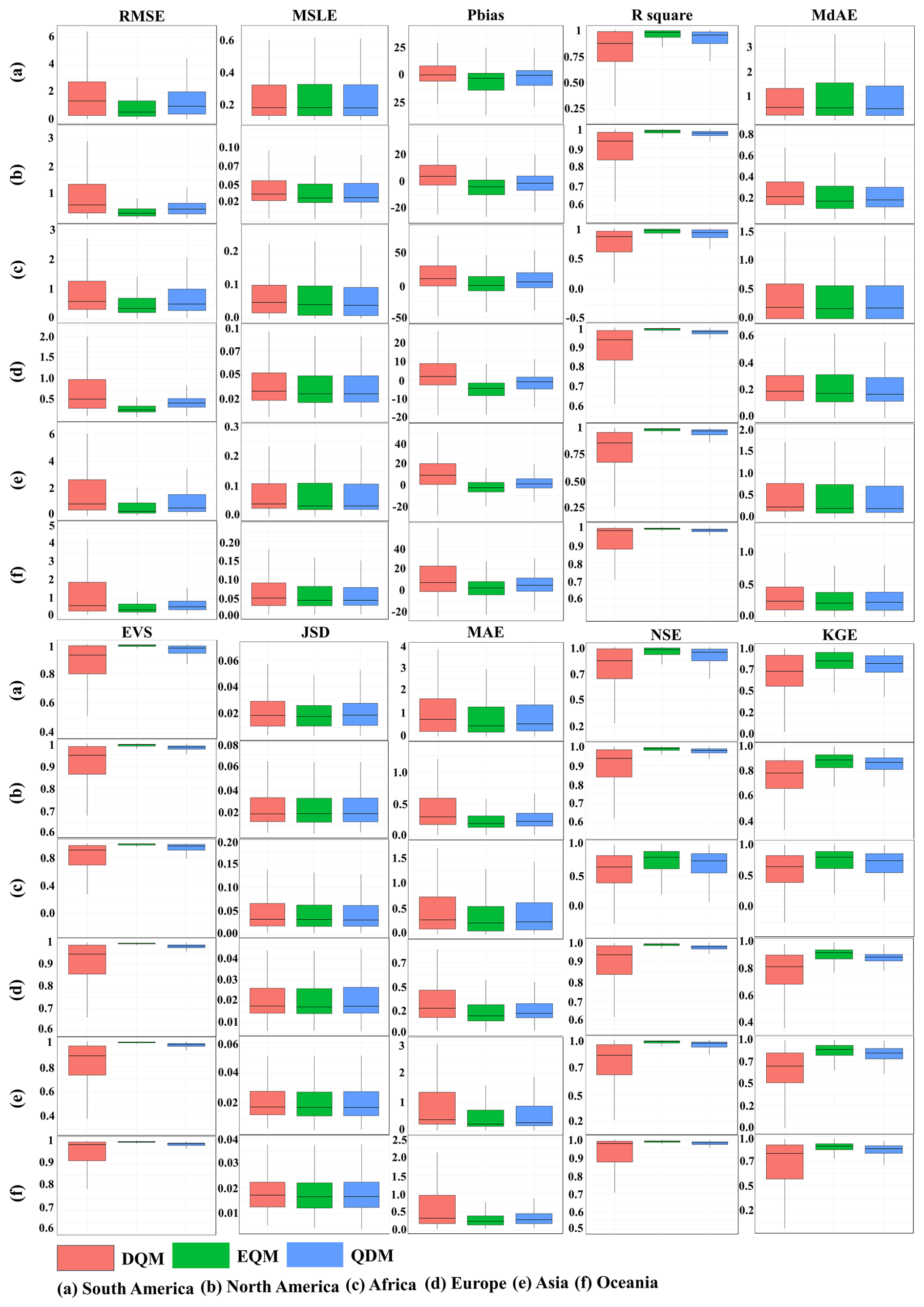
Figure 8 Performances of DQM, EQM, and QDM of historical period precipitation using boxplots based on ten evaluation metrics.

3.1.3 Comparison of reproducibility for extreme daily precipitation

This study also compared how well each bias correction method reproduces extreme precipitation by fitting a Generalized Extreme Value (GEV) distribution to the corrected daily values and then quantifying the distributional differences. Figure 9 shows the JSD of GEV fitted daily precipitation for DQM, EQM, and QDM on each continent. Across most continents, the median JSD for all three methods is extremely low (on the order of 10⁻⁴ to 10⁻⁵), and even the interquartile ranges fall within narrow bands indicating that statistically the GEV curves for DQM, EQM, and QDM are almost indistinguishable for historical data.

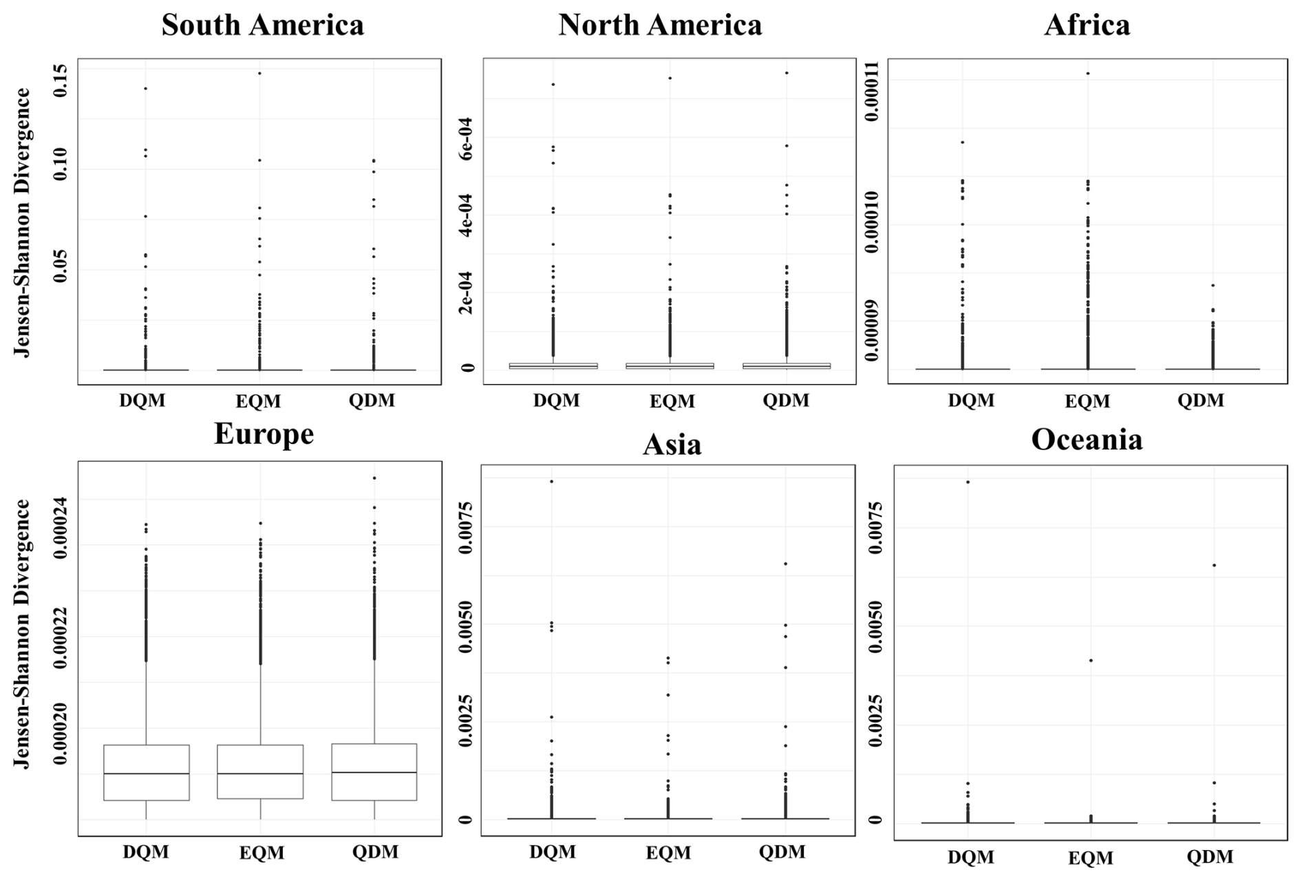
Figure 9 Comparison of distribution differences for GEV distribution using JSD across six continents.

Table S2 shows the results of a Friedman test and subsequent Wilcoxon signed rank pairwise comparisons for the ten highest daily precipitation values exceeding the 95th percentile on each continent. The Friedman test yielded a p-value of 4.5399 × 10⁻⁵, indicating a highly significant difference and that at least one of the three quantile-mapping methods differs systematically. All Wilcoxon pairwise comparisons between methods produced 0.00195 on every continent, demonstrating that no two bias-correction approaches generate equivalent extreme-precipitation estimates. Furthermore, the fact that both tests yielded identical results across continents indicates that the sign and rank structure of the three methods was the same in every continent, which in turn shows that the direction of the differences was consistent for each GCM.

Because the reproducibility of extreme values in the corrected GCM is essential for impact assessments, Fig. 10 presents the estimated probability density function (PDF) of precipitation values above the 95th percentile for the same GEV fit. Overall, DQM shows the highest probability density for extreme precipitation across all continents and has the widest tail, indicating that DQM boosts extreme events most aggressively. In contrast, EQM shows the lowest and narrowest density conservatively correcting extremes (often 5 %–8 % below DQM's values). QDM falls between EQM and DQM in most regions but remains closer to EQM.

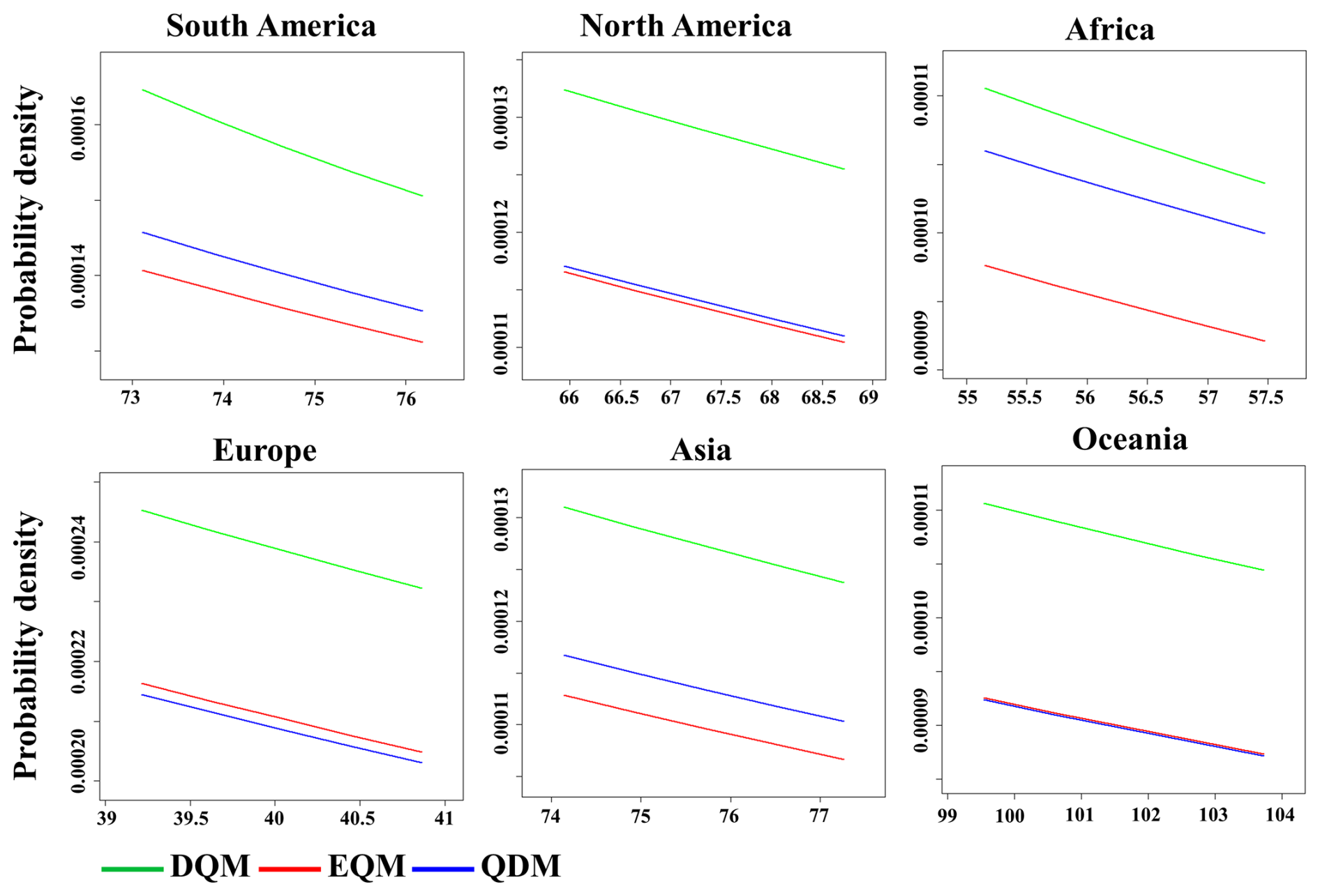
Figure 10 Comparison of probability densities for extreme precipitation values above the 95th percentile using GEV.

3.2 Prioritization of bias correction methods based on performance

3.2.1 Results of weight for evaluation metrics

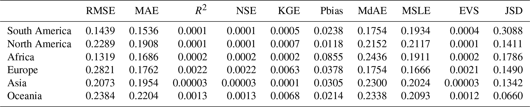
By conducting Friedman and Wilcoxon tests on the evaluation metrics, this study confirms that the observed differences in entropy-derived weights are statistically significant. In this study, the weights were calculated by applying entropy theory to the evaluation metrics used in the TOPSIS analysis, and the results are presented in Table 3. JSD had the highest weight in South America because the estimated JSD from 11 CMIP6 GCMs was an important metric for evaluating model performance differences. These results indicate that the differences between distributions are significant. On the other hand, EVS and NSE in South America had very low weights, suggesting that the variability and efficiency of precipitation were considered less important than other indicators. For North America, the RMSE, MSLE, and MAE metrics were of significant importance, as evidenced by their high weights. These error metrics revealed substantial regional differences. In contrast, EVS carried a negligible weight, suggesting it was less important in explaining variability in North America. For Africa, MdAE and JSD metrics were of considerable importance, as indicated by their high weights. These metrics were key evaluation factors in Africa. Conversely, EVS carried a low weight, suggesting it was considered relatively less important. RMSE had the highest weight in Europe, and KGE also had a relatively high weight, indicating that these metrics were considered important evaluation criteria in Europe. In Asia, MAE and MSLE had high weights, suggesting that these metrics were important evaluation metrics. On the other hand, EVS and NSE were considered less important due to their low variability. In Oceania, high weights were assigned to JSD, KGE, RMSE, and MAE, suggesting that these metrics are critical for evaluating model performance. On the other hand, R² and NSE were assigned low weights.

Table 3 Entropy-based weights for evaluation metrics across different continents.

3.2.2 Selection of the best bias correction method based on TOPSIS

Figures 11 and S2 present the best bias correction method selected for each continent using the TOPSIS approach. In Fig. 11, the spatial distribution of the most effective bias correction method across the grid points of each continent is shown. Figure S2 shows the number of grid points selected for each QM method. In South America, EQM was chosen as the best method in most grid points, with EQM being selected in over 1500 grid points. In contrast, QDM was selected in fewer than 700 grid cells, making it the least chosen method in South America. Across all continents except South America, EQM was selected as the best model in the majority of grid cells, with the number of selected grid points (North America: 7583; Africa: 2879; Europe: 2719; Asia: 8793; and Oceania: 1659). On the other hand, DQM was the least chosen method across all continents. For QDM, although it was the second most selected method across all continents except South America, the difference in the number of grid points between QDM and EQM is significant.

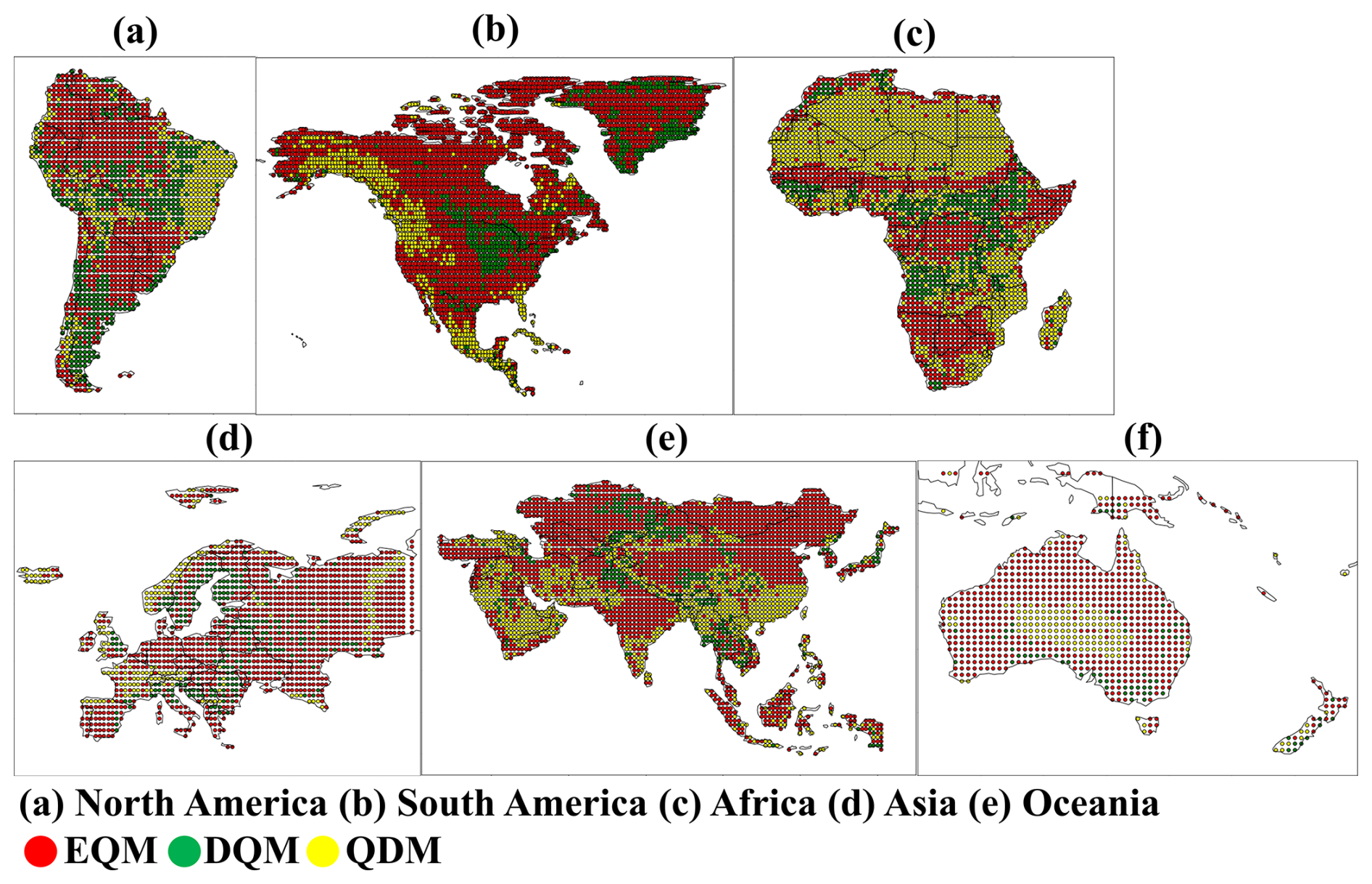
Figure 11 Spatial distribution for selected best bias correction methods across continents using TOPSIS.

3.3 Uncertainty quantification of bias corrected daily precipitation

3.3.1 Uncertainty by model

This study quantifies the daily precipitation uncertainty of 11 CMIP6 GCMs, corrected using three different BMA methods. Figure 12 shows the distribution of GCM weight variances calculated by BMA across six continents. In South America, the highest weight variance was observed mainly in DQM. EQM showed high weight variance in the northern region but lower variance than DQM in most other regions. QDM exhibited the lowest weight variance, with values less than 0.00113 in most regions. In North America, EQM had the lowest weight variance, with values between 0.00055 and 0.00024 in most regions. QDM showed the lowest model uncertainty across North America, with more regions where weight variances were closer to 0 than the other methods. On the other hand, DQM exhibited high weight variance overall, with exceptionally high model uncertainty in the northeast and southern regions. In Africa, EQM's weight variance was estimated to be low overall, resulting in low model uncertainty in most regions. For QDM, weight variance was low in some regions but higher than 0.00113 in others. DQM showed high weight variance in most regions except for the northern area, indicating high model uncertainty across the continent. EQM's weight variance was the lowest in Europe compared to the other methods, with weight variances close to 0 across the continent. QDM also showed low weight variance overall, though higher than EQM. DQM exhibited high weight variance in most regions except for Central Europe. In Asia, EQM showed low weight variance in most regions except Southeast Asia. QDM's weight variance was similar to EQM's, though some regions had higher model uncertainty. DQM showed high weight variance in most regions except for some Southwest and North Asian areas. For Oceania, the weight variances of EQM and DQM were mainly similar, but DQM showed a higher weight variance overall.

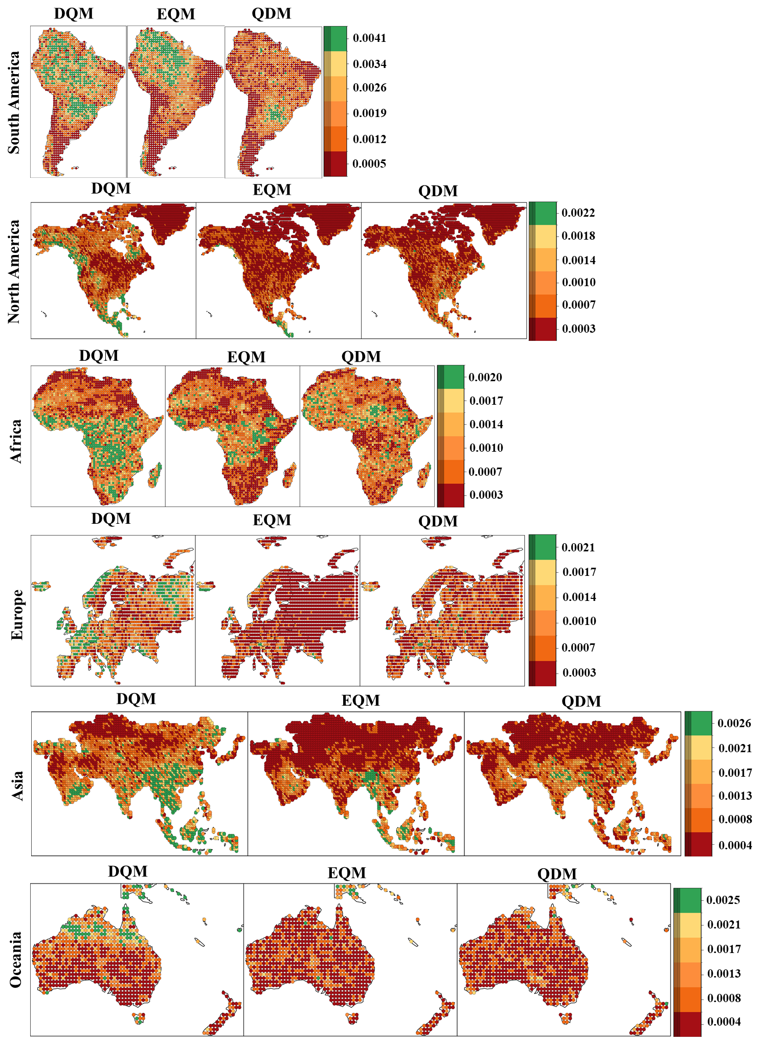
Figure 12 Spatial distribution of weight variance across continents for bias corrected CMIP6 GCMs using BMA.

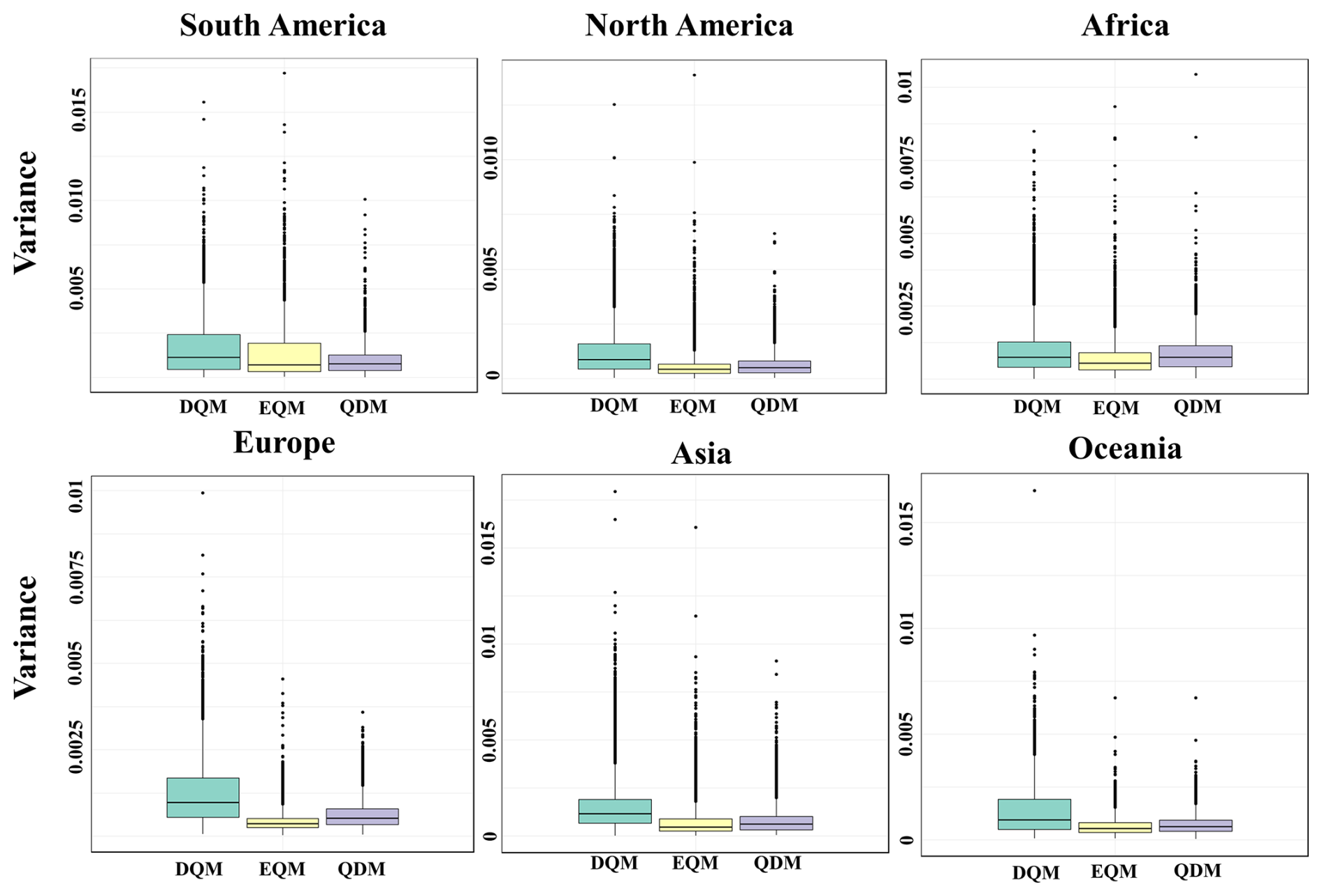
Figure 13 shows the distribution of GCM weight variances calculated using BMA across six continents, presented as boxplots. Overall, EQM has the smallest weight variance, and QDM has the second smallest weight variance on all continents except South America. In contrast, in South America, QDM has the smallest weight variance, and EQM has the second smallest. DQM consistently has the largest weight variance across all continents, indicating the highest model uncertainty.

Figure 13 Weight variance for bias correction methods across six continents using box plots.

3.3.2 Uncertainty by ensemble prediction

A daily precipitation ensemble for the historical period was generated using BMA on 11 CMIP6 GCMs, and the standard deviation of daily precipitation by continent is presented as shown in Fig. 14. Overall, the ensemble predicted using EQM provided stable precipitation projection with low standard deviations across most continents. The QDM ensemble showed similar results to EQM for most continents except Oceania, but the standard deviations were slightly higher. On the other hand, the ensemble using DQM exhibited higher standard deviations than the other methods for all continents and had the largest prediction uncertainty. In Oceania, the ensembles predicted by the three methods showed similar results. However, the prediction uncertainty was estimated to be lower in the order of EQM, DQM, and QDM due to slight differences.

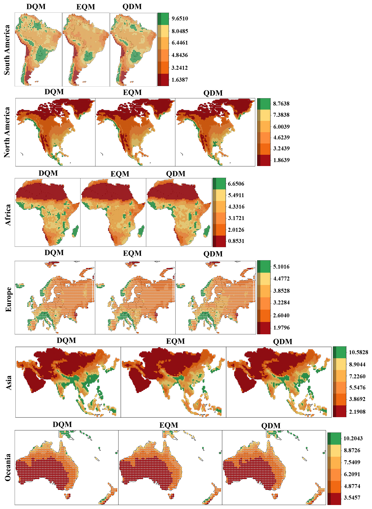
Figure 14 Spatial distribution of standard deviation for daily precipitation across continents for bias corrected CMIP6 GCMs using BMA.

Figure 15 shows the standard deviation of daily precipitation for the ensemble forecasted by BMA using three methods, DQM, EQM, and QDM, in a boxplot for each continent. Visually, EQM tends to show the lowest medians across continents, QDM appears slightly higher, and DQM tends to show the highest medians. The interquartile ranges overlap broadly within most continents and the differences in medians are small in magnitude.

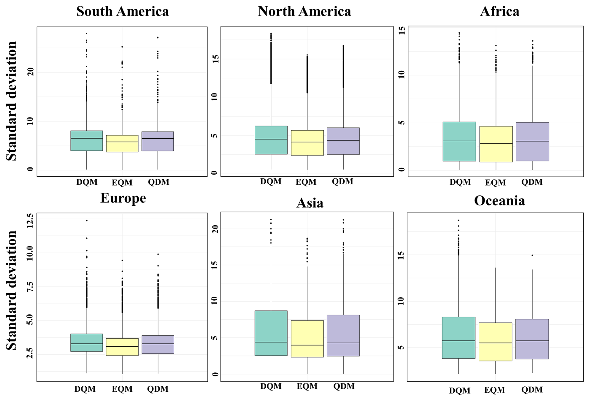
Figure 15 Spatial distribution of standard deviation for daily precipitation across continents for bias corrected CMIP6 GCMs using BMA.

3.4 Evaluation of bias correction methods using CI

3.4.1 Results of CI by each weighting case

This study compared three QM methods by generating a CI based on three cases of weighting values that considered both model performance and uncertainty. Figs. 16, S3, and S4 show the comprehensive indices calculated by applying equal weights and weights emphasizing performance and uncertainty, respectively.

EQM showed the highest CI across all continents when equal weights were applied. However, the index was lower in southern Europe and southeastern North America, but it calculated high values in most other regions. QDM showed high index values in some regions, although they were lower than those of EQM. For example, the CI results were high in the northern and western parts of North America and the central part of Europe. On the other hand, DQM was generally unsuitable in most regions but showed a relatively high index in Oceania.

When weights that emphasized performance were applied, DQM showed a high index in the central part of South America but low performance in most continents. Nevertheless, DQM showed a better index than QDM in some parts of Oceania. EQM showed the best index across most continents. While QDM was less suitable than EQM, it was still evaluated as a useful method in some continents.

Even when applying weights that increased the emphasis on uncertainty, similar results were obtained with the other weighting values. In particular, EQM was evaluated as the most suitable model across all continents, while DQM showed the opposite results.

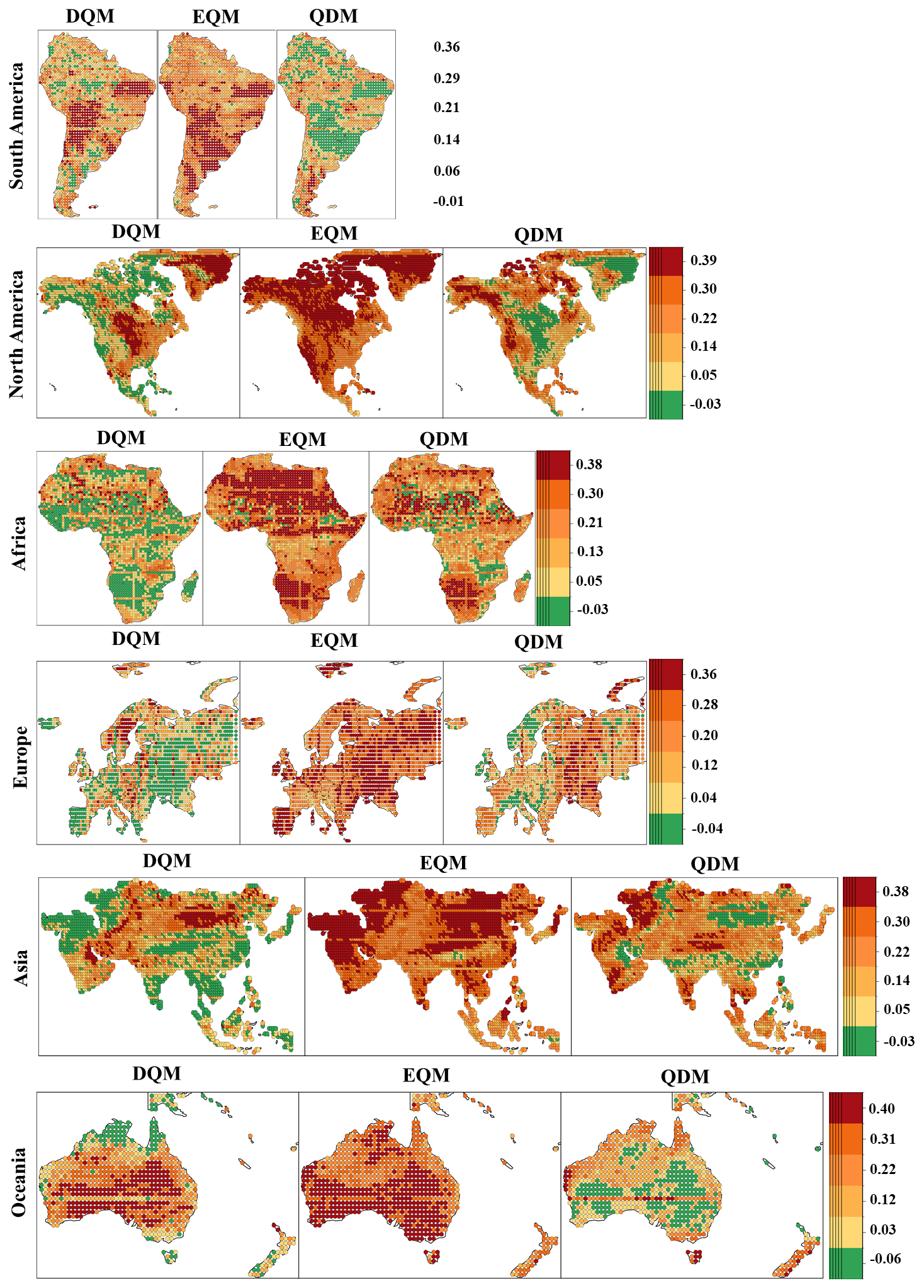
Figure 16 Spatial distribution of comprehensive indices for bias correction methods with equal weights (α: 0.5, β: 0.5) across continents

Figure 17 presents a comparison of the comprehensive indices for three QM methods with different weights for each continent using box plots. Overall, all methods showed higher indices than the other weighting values in the values that emphasized more weight on performance. In all weighted values, DQM showed the lowest indices in all continents except for South America and Oceania, where it was slightly higher or similar to QDM. EQM showed the best composite indices in all continents, outperforming performance and uncertainty. QDM showed high comprehensive indices in most continents, and the gap with EQM narrowed significantly in the weighting values that emphasized performance more. Nevertheless, QDM overall had lower comprehensive indices than EQM.

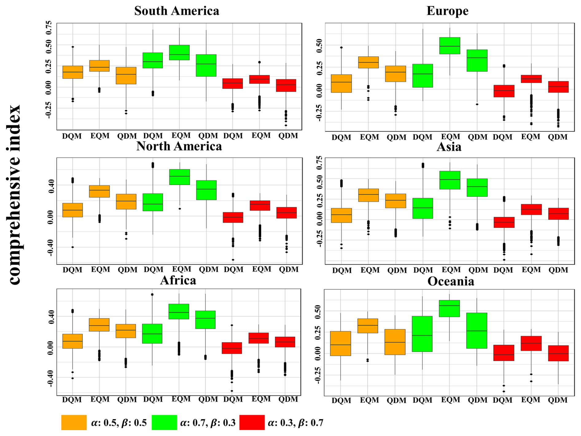
Figure 17 CI for three bias correction methods across continents with varying weights on performance and uncertainty.

Under the three weighting scenarios defined in the main text, the Friedman test produced p-values effectively rounded to zero for every continent, indicating highly significant differences among DQM, EQM, and QDM (Table S3 in the Supplement). Subsequent pairwise Wilcoxon tests showed that most method comparisons remained significant across all regions. The only notable exception occurred in Oceania under equal weighting, where the p-value of 3.93 × 10⁻¹ failed to reach significance at the 0.05 level. These findings demonstrate that, aside from that single case in Oceania, the choice of scenarios exerts a statistically significant impact on composite scores across all continents.

3.4.2 Selection of best bias correction method

Based on the CI, this study selected the best bias correction method for each continent. Figure 18 shows how the best bias correction method was selected for each continent by applying various weighting values of the CI. Overall, EQM was selected as the best correction method for most continents in all weighting values and was selected more than other methods in North America, Europe, Asia, and Oceania. DQM was selected the least in most continents except for South America and Oceania, and the number of selected grids tended to decrease as the weighting for uncertainty increased. QDM was selected as the best bias correction method in western North America, southern and eastern Africa, and northern Europe. In addition, QDM was selected the most in Southeast Asia in all weighting values.

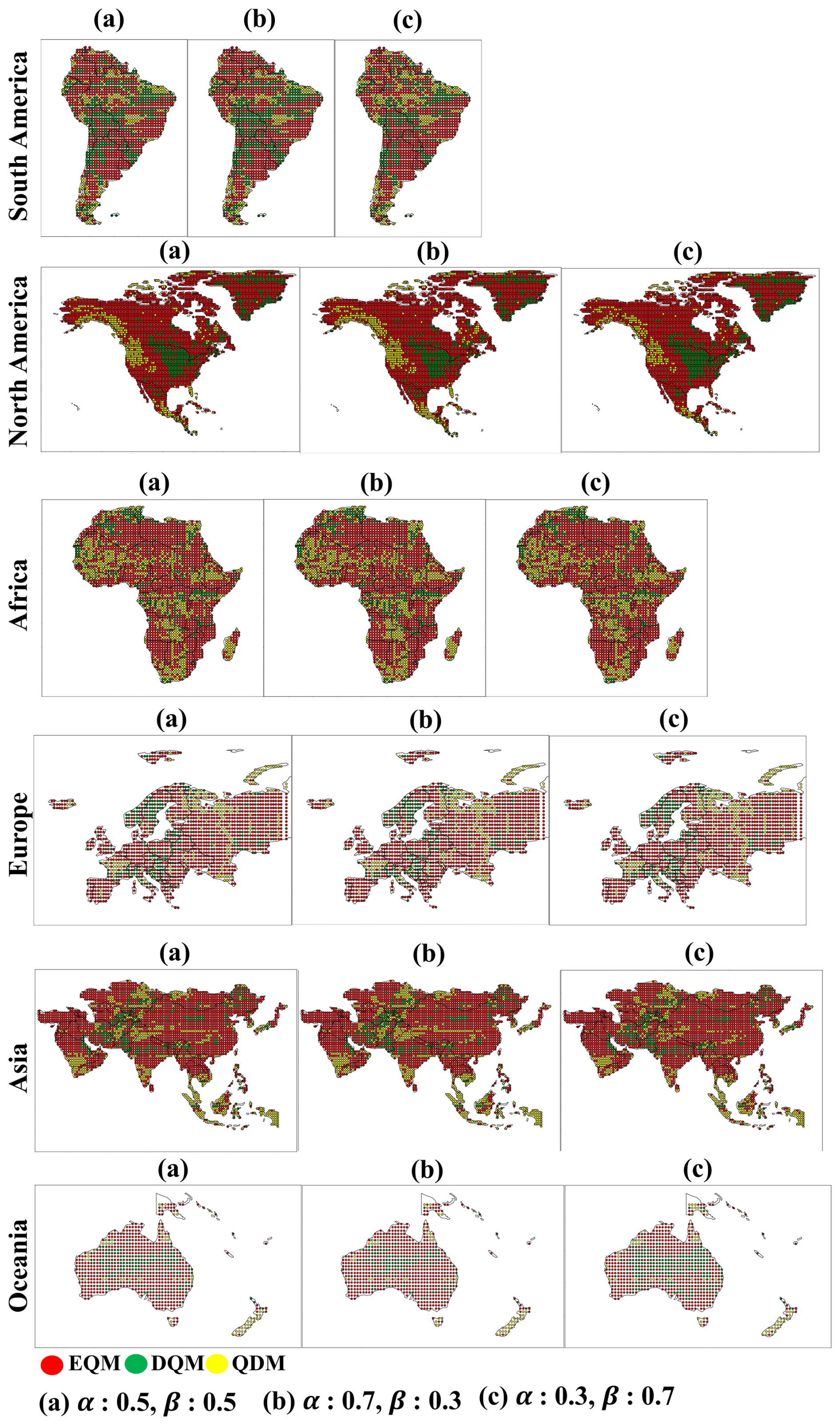
Figure 18 Selection of best bias correction methods across continents based on CI depending on weighting values.

Figure 19 shows the number of selected grids for the best bias correction method across continents based on three weighting values. Overall, EQM was the most frequently selected method across all weighting values, demonstrating superior performance across all continents compared to the other methods. Interestingly, as the weight for uncertainty increased, the number of grids where EQM was selected also increased, while the number decreased as the weight for performance increased. In contrast, QDM was chosen as the second-best method on most continents, except for South America and Oceania. The number of selected grids for QDM slightly increased as the performance weight increased. DQM was the least selected method across most continents, indicating that it was the least suitable overall.

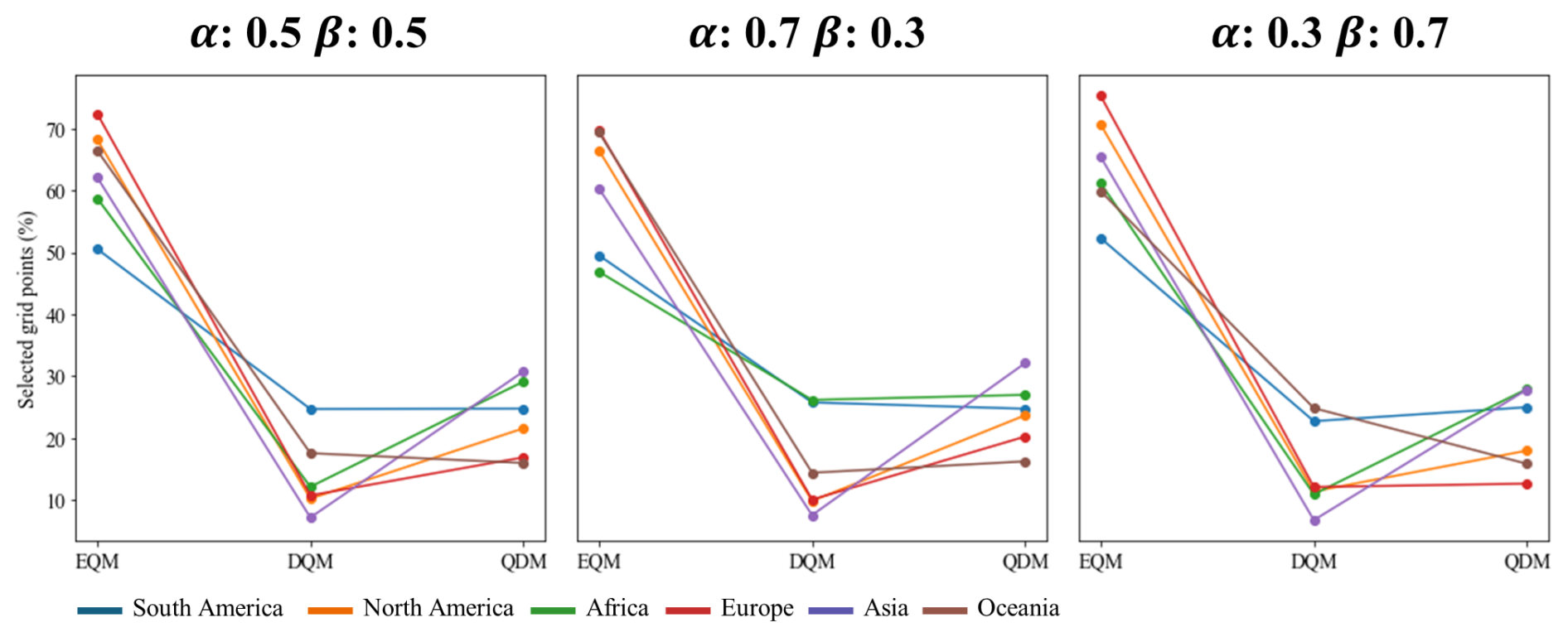
Figure 19 Ratios of selected grids for best bias correction methods across continents based on different weighting values.

4 Discussion

Bias correction methods are widely used in correcting GCM outputs, and previous studies have compared the performance of various methods (Homsi et al., 2019; Saranya and Vinish, 2021). Among these, Quantile Mapping (QM) has consistently shown superior performance compared to other methods, making it a widely used approach for bias correction. In particular, QDM, EQM, and DQM, which are the focus of this study, are frequently employed in research exploring and applying climate change projections based on GCM outputs (Cannon et al., 2015; Switanek et al., 2017; Song et al., 2022a). Analyzing the strengths and limitations of these three methods will provide valuable insights for climate researchers, enabling them to choose the most suitable bias correction method for specific regions. In this context, this study further evaluates the performance of QDM, EQM, and DQM, especially for daily precipitation, and investigates how these methods perform across different regions. Unlike previous studies that focused on the performance of bias correction methods (Song et al., 2024; Teutschbein and Seibert, 2012; Smitha et al., 2018), this study suggests a CI that integrates the performance and uncertainty metrics. This approach enhances the robustness of bias correction method selection and provides a more holistic evaluation framework. This section discusses the strengths and weaknesses of each method from various perspectives to provide a more balanced assessment.

4.1 Evaluation of bias correction methods performance

The daily precipitation corrected by the three QM methods outperformed the raw GCM data (see Fig. 1). All three methods, as evidenced by the Taylor diagram, demonstrated overall stronger performance than the raw GCM and consistently produced good results across various regions. Nonetheless, the performance of the bias-corrected GCMs clearly differs. This highlights the need to use multiple performance metrics to fully understand the strengths and weaknesses of the three QM methods, as relying on a single analysis or macroscopic perspective can overlook important details. From this perspective, many studies have emphasized the application of a multifaceted analysis in selecting bias correction methods (Homsi et al., 2019; Cannon et al., 2015; Berg et al., 2022; Song et al., 2023). The spatial distribution of correction performance, as discussed in Sect. 3.1.2, varies significantly by continent. Figures 2 to 7 reveal that the evaluated metrics differ across continents, underscoring the importance of region-specific correction methods. This finding aligns with Song et al. (2023), highlighting the importance of selecting appropriate correction methods based on the precipitation distribution at observation sites. Moreover, studies such as Homsi et al. (2019) and Saranya and Vinish (2021) also emphasize the variability in bias correction performance depending on the regional climate and data characteristics, reinforcing the need for tailored approaches. Of course, the three QM methods showed high performance across most continents, effectively correcting the biases in daily precipitation from GCMs. However, the corrected daily precipitation varies subtly among the three methods, with these differences becoming more pronounced in extreme events or specific evaluation metrics. For example, the three QM methods tend to perform less effectively in regions with high precipitation, but their performance also varies by grid (e.g., southern India in Asia: RMSE; central Oceania: Pbias and EVS; central Europe: Pbias, MdAE, and KGE). While EQM performs well across most continents, DQM and QDM show superior results in specific regions. Similar results were made by Cannon et al. (2015), which highlighted differences in the performance of bias correction methods, particularly in handling extreme precipitation events. QDM's error-related metrics (South America: RMSE, MAE, and MSLE) are nearly identical to EQM's, yet QDM outperforms EQM regarding MdAE on more grids. These findings suggest that a more nuanced and detailed analysis of precipitation corrected by GCMs is necessary, aligning with the conclusions of Gudmundsson et al. (2012), which emphasize that the effectiveness of bias correction methods can vary significantly depending on local climate characteristics, highlighting the importance of selecting appropriate methods for each region. These results suggest a more detailed precipitation analysis from corrected GCMs is needed.

This study compared the three QM methods for daily precipitation events above the 95th percentile (extreme precipitation) using the GEV distribution, as shown in Fig. 10. The results indicate that DQM tends to correct more extreme precipitation events than QDM, aligning with previous findings that DQM captures a broader range of extremes. The unique characteristics of DQM caused these results. DQM overestimated the corrected extreme precipitation due to the relative variability in the data introduced through detrending, and the subsequent reintroduction of the long-term mean during the correction step widened the range of extreme precipitation, leading to overestimation compared to the reference data in areas with high variability. At the same time, QDM and EQM take a more conservative approach (as noted in previous studies such as Cannon et al., 2015). These findings suggest that EQM and QDM may be more suitable in regions vulnerable to floods and extreme weather events that require a more balanced and cautious approach. However, when comparing the differences in GEV distributions, there was no significant difference between methods in regions like Oceania and Europe (see Fig. 10). These results imply that EQM can better handle extreme values or outliers in the data by directly comparing and correcting past and future distributions. In particular, EQM is consistent with previous studies in that it more accurately corrects observed distributions in non-stationary and highly variable climate variables, such as precipitation (Themeßl et al., 2012; Maraun, 2013; Gudmundsson et al., 2012). These positive aspects are mainly due to EQM's ability to align the empirical ECDFs of reference and model data across all quantiles, allowing it to correct biases with high precision at both central tendencies and extremes. Although there are significant advantages in observing the results of the correction method in detail from various perspectives, presenting these results without integrating them into a reasonable framework can increase confusion and uncertainty in climate change research (Wu et al., 2022). Therefore, it is essential to introduce a structured framework such as MCDA to provide a single integrated result.

4.2 Uncertainties of model and ensemble prediction in bias correction methods

In climate modeling, quantifying uncertainty is essential to assess the reliability of bias-corrected precipitation data. This study applied BMA to quantify the uncertainty of three QM methods on a continental basis, addressing both model-specific and ensemble prediction uncertainties. Similar to the findings by Cannon et al. (2015), this analysis demonstrates how different bias correction methods yield varying uncertainty levels based on the underlying climate models. Notably, EQM showed the lowest weight variance across most continents, which means that the inter-model uncertainty for 11 GCMs corrected by EQM is lower than that of the other QM methods. The low uncertainty associated with EQM aligns with previous studies like Themeßl et al. (2012), which found that EQM consistently reduced discrepancies between modeled and observed data across regions. EQM's ability to manage extreme precipitation and anomalous values based on observed distributions contributes to its reliability, a feature also emphasized by Gudmundsson et al. (2012). On the other hand, DQM showed the highest weight variance across all continents, indicating more significant uncertainty when applied to various GCMs. This uncertainty was particularly pronounced in regions with complex climate conditions, such as Southeast Asia, East Africa, and the Alps in Europe. These results align with Berg et al. (2022), who highlighted DQM's limitations in capturing long-term climate trends and extreme events. The higher uncertainty associated with DQM suggests that, while its detrending process is effective in correcting the mean, it may struggle in regions dominated by nonlinear climate patterns, as it does not sufficiently account for all quantiles in the distribution, particularly extremes, as noted by Cannon et al. (2015). QDM, though showing lower weight variance than DQM, still demonstrated higher uncertainty than EQM in regions with diverse climate characteristics. These results are consistent with the study of Tong et al. (2021), suggesting that QDM performs better under moderate precipitation scenarios. However, the uncertainty may increase under highly variable or extreme weather conditions. Furthermore, this study extended the uncertainty analysis to ensemble predictions, calculating the standard deviation of daily precipitation for each continent using BMA. The EQM-based ensemble consistently exhibited low standard deviations across all continents, indicating that EQM offers the most stable and reliable precipitation predictions. This finding echoes the conclusions drawn by Teng et al. (2015), where EQM provided more accurate and less uncertain projections. In contrast, DQM presented the most significant prediction uncertainty, reinforcing the need for caution when applying DQM in studies that require high-confidence data. These results emphasize the importance of weighing performance and uncertainty when choosing a suitable bias correction method. EQM's consistent performance in reducing uncertainty across model-specific and ensemble forecasts highlights its robustness as a preferred choice for climate research. However, the substantial uncertainty associated with DQM suggests that its use should be limited to regions where its detrending process can be beneficial. Overall, these findings stress the critical role of uncertainty quantification in climate change impact assessments and underscore the need for selecting bias correction methods based on a comprehensive evaluation of both performance and uncertainty.

4.3 Integrated assessment of bias correction methods

This study selected the optimal QM method for each continent based on the CI, which considers uncertainty and performance. The critical point is that uncertainty is decisive when selecting a bias correction method. As shown in Fig. 19, the optimal correction method varies depending on the continent, and the selected method also changes depending on the weight. These results suggest that uncertainty still exists, as Berg et al. (2022) pointed out, and that uncertainty must be considered when selecting the optimal method. In other words, even if the QM method has high performance, it is difficult to make a reasonable selection if the uncertainty contained in the method is significant. Overall, EQM showed the highest CI value in all continents, which means that it provides the most balanced results in terms of performance and uncertainty. These results are consistent with previous studies (Lafon et al., 2013; Teutschbein and Seibert, 2012; Teng et al., 2015) that showed high precipitation correction accuracy and excellent performance, especially under complex climate conditions. QDM was evaluated highly in some regions but performed worse than EQM overall. Berg et al. (2022) also pointed out that QDM is superior in general climate conditions but may perform worse in extreme climate situations, suggesting that this may increase the uncertainty of QDM in extreme climates. DQM was evaluated as an unsuitable method in most regions due to low CI values, which is consistent with the limitations of DQM mentioned in Cannon et al. (2015) and Berg et al. (2022). It was confirmed that DQM performs relatively well in dry climates but may perform worse in various climate conditions. In addition, some differences were observed with the results based on TOPSIS. For example, DQM was selected more than QDM in South America, but when the uncertainty weight was applied, QDM was selected more. Conversely, in Oceania, QDM was selected more than DQM, but when the uncertainty weight was increased to 0.7, DQM was selected more. These results are consistent with those of Lafferty and Sriver (2023), showing that when significant uncertainty exists, uncertainty can be greater despite high bias correction performance.

5 Conclusions

This study corrected and compared historical daily precipitation from 11 CMIP6 GCMs using three QM methods. Eleven statistical metrics were used to evaluate the precipitation performance corrected by three QM methods, and TOPSIS was applied to select performance-based priorities. BMA was applied to quantify model-specific and ensemble prediction uncertainties. Additionally, suitable QM methods were selected and compared using a CI that integrates TOPSIS performance scores with BMA uncertainty metrics. The conclusions of this study are as follows:

1. EQM showed the highest overall index across all continents, indicating that it provides the most balanced approach in terms of performance and uncertainty.

2. DQM effectively reproduced the dry climate in North Africa and parts of Central and Southwest Asia but showed the highest uncertainty across all continents. These results suggest that DQM may lose some long-term trend information, making it less reliable in regions prone to extreme weather events.

3. QDM performed better in certain regions, such as Southeast Asia, and was selected more often than DQM when uncertainty was given greater weight. QDM may be a promising alternative in areas where uncertainty plays a significant role.

4. Selecting an appropriate QM is required for high performance, and significant uncertainty can complicate rational decision-making. Therefore, a multifaceted approach considering performance and uncertainty is essential in climate modeling.

In conclusion, EQM has emerged as the preferred method due to its balanced performance, but this study emphasizes the importance of regional assessment and careful consideration of uncertainty when selecting a QM method. Furthermore, EQM is the most balanced method regarding performance and uncertainty and will likely be preferred in future climate modeling studies. However, there may be more suitable QM methods depending on the region, and a comprehensive evaluation with various weights is needed. Therefore, when establishing climate change response strategies or policy decisions, it is essential to take a multifaceted approach that considers uncertainty together rather than relying on a single indicator or performance alone. It will enable more reliable predictions and better decision-making. Future research should integrate greenhouse gas scenarios to improve the accuracy of climate predictions and provide a more comprehensive understanding of future climate risks. Furthermore, more bias correction methods should be used to extend the robustness of CI.