Moving beyond post hoc explainable artificial intelligence: a perspective paper on lessons learned from dynamical climate modeling

AI models are criticized as being black boxes, potentially subjecting climate science to greater uncertainty. Explainable artificial intelligence (XAI) has been proposed to probe AI models and increase trust. In this review and perspective paper, we suggest that, in addition to using XAI methods, AI researchers in climate science can learn from past successes in the development of physics-based dynamical climate models. Dynamical models are complex but have gained trust because their successes and failures can sometimes be attributed to specific components or sub-models, such as when model bias is explained by pointing to a particular parameterization. We propose three types of understanding as a basis to evaluate trust in dynamical and AI models alike: (1) instrumental understanding, which is obtained when a model has passed a functional test; (2) statistical understanding, obtained when researchers can make sense of the modeling results using statistical techniques to identify input–output relationships; and (3) component-level understanding, which refers to modelers' ability to point to specific model components or parts in the model architecture as the culprit for erratic model behaviors or as the crucial reason why the model functions well. We demonstrate how component-level understanding has been sought and achieved via climate model intercomparison projects over the past several decades. Such component-level understanding routinely leads to model improvements and may also serve as a template for thinking about AI-driven climate science. Currently, XAI methods can help explain the behaviors of AI models by focusing on the mapping between input and output, thereby increasing the statistical understanding of AI models. Yet, to further increase our understanding of AI models, we will have to build AI models that have interpretable components amenable to component-level understanding. We give recent examples from the AI climate science literature to highlight some recent, albeit limited, successes in achieving component-level understanding and thereby explaining model behavior. The merit of such interpretable AI models is that they serve as a stronger basis for trust in climate modeling and, by extension, downstream uses of climate model data.

1 Introduction

Machine learning (ML) is becoming increasingly utilized in climate science for tasks ranging from climate model emulation (Beucler et al., 2019), to downscaling (McGinnis et al., 2021), forecasting (Ham et al., 2019), and analyzing complex and large datasets more generally (for an overview of ML in climate science, see Reichstein et al., 2019; Molina et al., 2023; de Burgh-Day and Leeuwenburg, 2023). Compared with physics-based methods, ML, once trained, has a key advantage: computational expense reduced by orders of magnitude. Along with the advantages of ML come challenges such as assessing ML trustworthiness. For example, scientists often do not understand why a neural net (NN) gives the output that it does because the NN is a “black box.”¹

To build trust in ML, the field of explainable artificial intelligence (XAI) has become increasingly prominent in climate science (Bommer et al., 2023). Sometimes referred to as “opening the black box,” XAI methods consist of additional models or algorithms intended to shed light on why the ML model gives the output that it does. For example, Labe and Barnes (2021) use an XAI method, layer-wise relevance propagation², and find that their NN heavily relies on data points from the North Atlantic, Southern Ocean, and Southeast Asia to make its predictions.

While XAI methods can produce useful information about ML model behaviors, these methods also face problems and have been subjected to critique. As Barnes et al. (2022) note, XAI methods “do not explain the actual decision-making process of the network” (p. 1). Additionally, different XAI methods applied to the same ML model prediction have been shown to exhibit discordance, i.e., yielding different and even incompatible “explanations” for the same ML model (Mamalakis et al., 2022b). Discordance in XAI is not unique to climate science. Krishna et al. (2022) find that 84 % of their interviewees (ML practitioners across fields who use XAI methods) report experiencing discordance in their day-to-day workflow, and when it comes to resolving discordance, 86 % of their online user study responses indicate that ML practitioners either employed arbitrary heuristics (e.g., choosing a favorite method or result) or simply did not know what to do.

As Molina et al. (2023) note, “identifying potential failure modes of XAI, and uncertainty quantification pertaining to different types of XAI methods, are both crucial to establish confidence levels in XAI output and determine whether ML predictions are `right for the right reasons”' (p. 8). Rudin (2019) argues that, instead of attempting to use XAI to explain ML models post hoc, scientists ought to build interpretable models informed by domain expertise from the outset. Speaking about explainability in particular, Rudin writes, “many of the [XAI] methods that claim to produce explanations instead compute useful summary statistics of predictions made by the original model. Rather than producing explanations that are faithful to the original model, they show trends in how predictions are related to the features” of the model input Rudin (2019, p. 208).

Regardless, XAI methods will likely continue to be widely applied due to ease of use and as benchmark metrics for XAI methods are proposed and implemented (Hedström et al., 2023; Bommer et al., 2023). In some cases, XAI methods are applied with great success; e.g., Mamalakis et al. (2022b) found that the input × gradient method fit their ground-truth model with a high degree of accuracy. However, we believe that more progress can be made in establishing trust in ML-driven climate science, especially as an increasing number of researchers start incorporating ML into climate research (see Fig. 1).

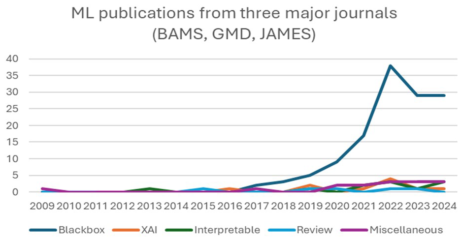
Figure 1 Trends of publications related to AI, ML, or XAI from three major journals (BAMS, GMD, JAMES) based on 178 references acquired from the Web of Science on 17 October 2023. There are two notable results. Result 1: AI and ML publications are predominantly “black box applications” (132 out of 178 records). Both XAI and interpretable AI emerged in 2020 and are in their infancy by comparison. Result 2: black box AI applications are on the rise. (The dip in 2023 and 2024 can be explained by data collection methods. Note that this is not intended as a systematic survey of AI in climate science. One key shortcoming is that the data excluded journals such as Artificial Intelligence for Earth Systems (AIES) because the Web of Science did not include AIES at the time of data collection.) See the Supplement for a full data description.

In this review and perspective paper, we target readers with expertise in traditional approaches for climate science (e.g., development, evaluation, and application of traditional Earth system models) who are starting to utilize ML in their research and who may see XAI as a tempting way to gain insight into model behavior and to build confidence. From this perspective, we draw from some ideas in the philosophy of science to recommend that such researchers leverage the expanding array of freely available ML resources to move beyond post hoc XAI methods and aim for component-level understanding of ML models. By “component” we mean a functional unit of the model's architecture, such as a layer or layers in a neural net. By “understanding” we mean knowledge that could serve as a basis for an explanation about the model. We distinguish between three levels of understanding.

• Instrumental understanding involves knowing that the model performed well (or not), e.g., knowing its error rate on a given test.

• Statistical understanding means being able to offer a reason why we should trust a given ML model by appealing to input–output mappings. These mappings can be retrieved by statistical techniques.

• Component-level understanding means being able to point to specific model components or parts in the model architecture as the cause of erratic model behaviors or as the crucial reason why the model functions well.

These levels concern the degree to which complex models are intelligible or graspable to scientists (De Regt and Dieks, 2005; Knüsel and Baumberger, 2020; De Regt, 2017). Therefore, our proposal has a narrower but deeper focus than recent philosophy of science accounts of understanding climate phenomena with or by using ML and dynamical climate models (Jebeile et al., 2021; Knüsel and Baumberger, 2020). We are concerned with understanding, diagnosing, and improving model behavior to inform model development.

Instrumental understanding, while clearly necessary, is fairly straightforward and is a prerequisite for any explanation of model behavior. It involves knowing the degree to which a model fits some data (Lloyd, 2010; Baumberger et al., 2017). It may also involve knowing whether the model both fits some data and agrees with simpler models about a prediction of interest or whether the model has performed well on an out-of-sample test (e.g., Hausfather et al., 2020) or according to other metrics (e.g., Gleckler et al., 2008).

However, in this review and perspective paper, we will only focus on the other two types of understanding. Statistical understanding can be gained via traditional XAI methods but does not require knowledge of the model's inner workings, i.e., its components and/or architecture (see Sect. 2 below). In contrast, component-level understanding does involve knowledge of the model's inner workings. Therefore, component-level understanding allows scientists to offer causal explanations that attribute ML model behaviors to its components. Scientists need to build and analyze their models in such a way that they can understand how distinct model components contribute to the model's overall predictive successes or failures rather than merely probing model data to yield input–output mappings. The latter is emblematic of traditional XAI methods.

Our recommendation to strive for component-level understanding is inspired by how dynamical climate models have been built, tested, and improved, such as those in the Coupled Model Intercomparison Project (CMIP). Therefore, a novel contribution of this paper is the linking of existing climate model development practices to practices that could be employed in ML model development.

In CMIP, when models agree on a particular result, scientists sometimes infer that the governing equations and prescribed forcings shared by the models are responsible for the models' similar results. As Baumberger et al. (2017) put it, “robustness of model results (combined with their empirical accuracy) is often seen as making it likely, or at least increasing our confidence, that the processes that determine these results are encapsulated sufficiently well in the models” (p. 11; see also Hegerl et al., 2007; Kravitz et al., 2013; Lloyd, 2015; Schmidt and Sherwood, 2015; O'Loughlin, 2021). Conversely, when climate models exhibit biases or errors, scientists can often point to specific parameterizations or sub-models as the likely cause (e.g., Gleckler et al., 1995; Pitari et al., 2014; Gettelman et al., 2019; Zelinka et al., 2020; O'Loughlin, 2023), although models can get the right answer for the wrong reasons (see, e.g., Knutti, 2008).

To be clear, there are limits to how much component-level understanding can be achieved in CMIP. Dynamical climate models exhibit fuzzy (rather than sharp) modularity, meaning that the behavior of a fully coupled model is “the complex result of the interaction of the modules – not the interaction of the results of the modules” (Lenhard and Winsberg, 2010, p. 256). Climate scientists are familiar with a related problem: the difficulty in explaining how climate models generate (or not) emergent phenomena like the Madden–Julian oscillation (Lin et al., 2024). Despite these difficulties, philosophers and other scholars of climate science have documented successes in attributing model behavior to individual model components in the climate science literature (Carrier and Lenhard, 2019; Frigg et al., 2015; Gettelman et al., 2019; Hall and Qu, 2006; Hourdin et al., 2013; Mayernik, 2021; Notz et al., 2013; O'Loughlin, 2023; Oreopoulos et al., 2012; Pincus et al., 2016; Touzé-Peiffer et al., 2020). These successes do not imply anything like a “full” or “complete” understanding of all model behavior; rather, the component-level understanding of climate model behavior comes in degrees (Jebeile et al., 2021).

Fortunately, we see component-level understanding exemplified in ML-driven climate science to some extent already (Beucler et al., 2019; Kashinath et al., 2021; Bonev et al., 2023; see Sect. 4 below). Indeed, the thinking behind physics-informed machine learning, which incorporates known physical relations into the models from the outset (Kashinath et al., 2021; Wang et al., 2022; Cuomo et al., 2022), often involves component-level understanding. Thus, our proposal is an endorsement of these ongoing best practices, a recognition of the relationship between the evaluation of dynamical models and data-driven models, and a warning about the limits of statistical understanding. In addition, there is a concurrent need to establish the trustworthiness of ML models as ML-driven climate science potentially becomes increasingly used to inform decision-makers (NSF AI Institute for Research on Trustworthy AI in Weather, Climate, and Coastal Oceanography (AI2ES), 2024). While decision-makers themselves do not need to understand exactly how a model arrives at the answer it does, they may desire an explanation of the model's behavior that comes from a credible expert. One way to establish credibility is to be able to explain ML model behavior by appealing to the inner workings of the model, which requires component-level understanding of the model. In this way, component-level understanding can serve as a basis for trust in ML-driven climate science.

The remainder of the paper is structured as follows. In Sect. 2, we give an overview of XAI in climate science and explain the idea of statistical understanding and how XAI can only give us statistical understanding. In Sect. 3, we detail the notion of component-level understanding and demonstrate it using examples from CMIP. In Sect. 4, we show how component-level understanding is achievable in ML. In Sect. 5, we conclude and make suggestions for ML-driven climate science, including describing some resources that interested readers might utilize to build the expertise in ML model design necessary to probe, build, and adapt models in a way that is amenable to component-level understanding.

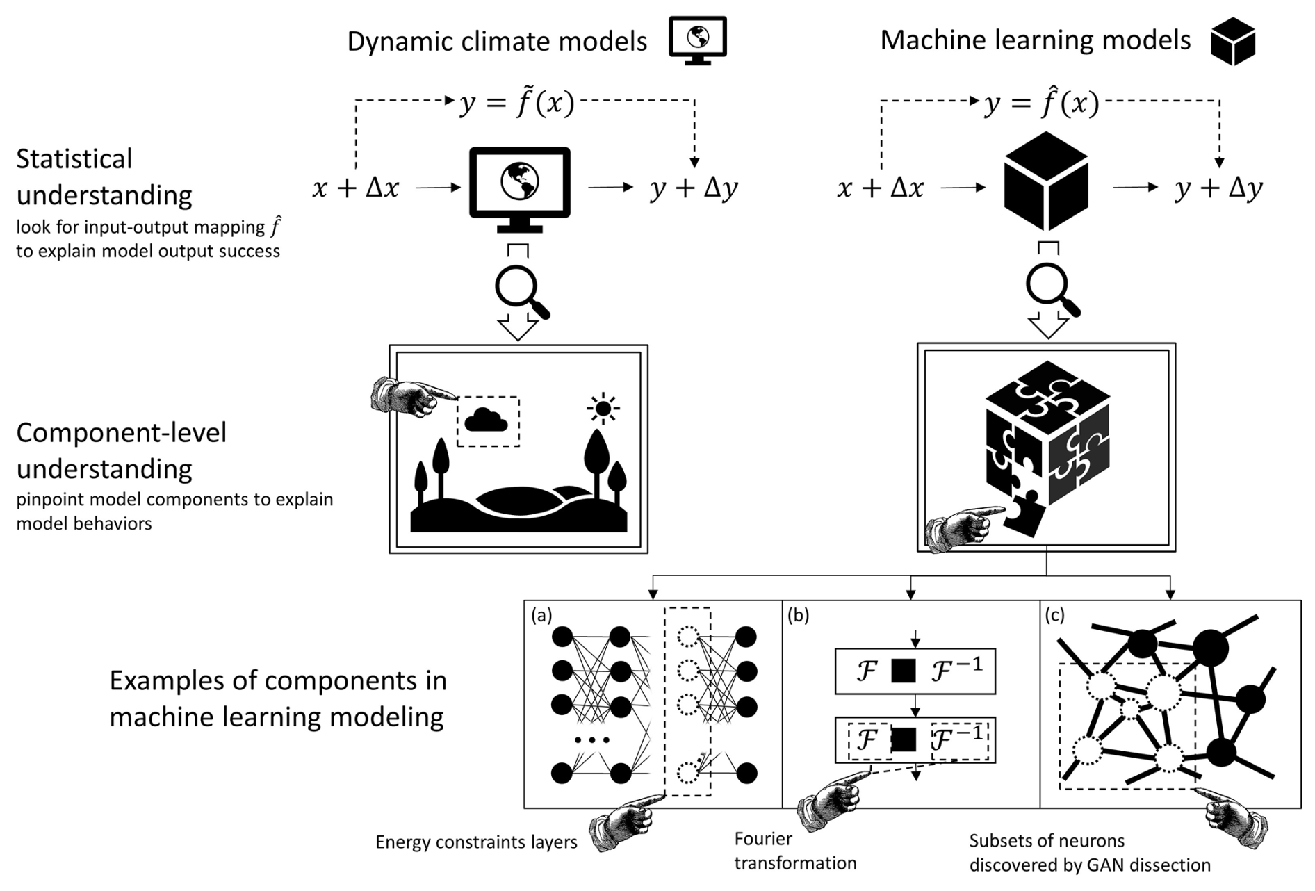
Figure 2 Scientists can obtain statistical understanding of models by seeking input–output mapping, e.g., via perturbation experiments. To acquire component-level understanding, one needs to be able to pinpoint specific components to explain models' erratic behaviors or successes. This has been done in dynamic climate modeling, e.g., by analyzing cloud parameterizations as a means to improve modeling outcomes. We offer three examples of component-level understanding in machine learning. In panel (a), Beucler et al. (2021) design layers of neurons in their neural network to enforce energy conservation and improve model outcome. In panel (b), Bonev et al. (2023) use spherical Fourier transformation to ensure that Fourier neural operators perform with climate data. In panel (c), Bau et al. (2018) use a method called GAN dissection to identify which subsets of neurons control parts of images that correspond to semantics (e.g., trees or doors). See Sect. 4 below for a discussion of these three examples.

2 Post hoc XAI in climate science and statistical understanding

XAI methods are intended to shed light on the behavior of complex opaque ML models. As Mamalakis et al. (2022a) put it, XAI “methods aim at a post hoc attribution of the NN prediction to specific features in the input domain (usually referred to as attribution/relevance heatmaps³), thus identifying relationships between the input and the output that may be interpreted physically by the scientists” (p. 316). XAI methods are typically applied to ML models which are multi-layer, convolutional, recurrent neural networks, and/or ensembles of decision trees (a common example of the latter is random forests).

The general idea behind XAI methods is to attribute the predictive success of the model's output (i.e., the model's prediction or decision) to subsets of its input in supervised ML. Broadly, there are two conceptual approaches to achieve this.⁴ One approach is perturbing the input data to figure out how the changes in input affect the output. The other approach studies the functional representation between input and output.

For the approach of perturbing the input, Local Interpretable Model-agonistic Explanation (LIME) is a method that first perturbs an input data point to create surrogate data near said data point. Then, after the trained ML model classifies the surrogate data, LIME fits a linear regression using classified surrogate data and measures how model output can be attributed to features of the surrogate data manifold. In this way, LIME attributes the predictive success for the actual data point to a subset of input features. Note that L stands for “local” because LIME, as a method, perturbs classification instances. For example, pixels, or clusters of pixels, of one image may be perturbed to create a surrogate instance. Then this surrogate instance is classified by the ML model in question to see how the output changes. LIME does not deal with all data points all at once.

Another commonly used method of the approach of perturbing input data is Shapley additive explanation (SHAP), which is based on calculating the Shapley values of each input feature. Shapley values are cooperative game theoretic measures that distribute gains or costs to members of a coalition. Roughly put, Shapley values are calculated by repeatedly randomly removing a member from the group to form a new coalition, calculating the consequent gains, and then averaging all marginal contributions to all possible coalitions. In the XAI context, input features will have different Shapley values, denoting their different contribution to the model's predictive success (see, e.g., Chakraborty et al., 2021; Cilli et al., 2022; Clare et al., 2022; Felsche and Ludwig, 2021; Grundner et al., 2022; Li et al., 2022; Xue et al., 2022).

The other approach relies on treating a trained black box model as a function to understand how the input–output mapping relationship is represented by this function. For example, vanilla gradient (also known as saliency) is an XAI method that relies on calculating the gradient of probabilities of output being in each possible category with respect to its input and back-propagating the information to its input. In this way, vanilla gradient quantifies the relative importance of each element of the input vector with respect to the output, thereby attributing the predictive success to subsets of input; see, e.g., Balmaceda-Huarte et al. (2023), Liu et al. (2023), and He et al. (2024).

Let us examine how XAI methods yield statistical understanding in a detailed example. González-Abad et al. (2023) use the saliency method to examine input–output mappings in three different convolutional neural nets (CNNs) which were trained and used to downscale climate data. They computed and produced accumulated saliency maps which account for “the overall importance of the different elements” of the input data for the model's prediction (p. 8). One of their results is that, in one of the CNNs, air temperature (at 500, 700, 850, and 1000 hPa) accumulates the highest relevance for predicting North American near-surface air temperature, although different regions are apparently more relevant than others to the models' predictions (see their Fig. 6, p. 12). In other words, it appeared that the CNN had correctly picked up on a relationship between coarse-resolution temperature at certain geopotential heights on the one hand and higher-resolution near-surface air temperatures on the other hand.

In this way, XAI methods yield information that can be helpful in making a model's results intelligible. For example, it puts a scientist in the position to say, “this model was picking up on aspects A, B, and C of the input data. These aspects contributed to prediction X, a prediction that seems plausible.” This exemplifies what we call “statistical understanding”, i.e., being able to offer a reason why we should trust a given ML model by appealing to statistical mappings between input and output. Statistical techniques are often used to obtain these mappings by relating variations in input to variations in output. Post hoc XAI methods can typically yield this type of understanding. Note that this is not the same as explaining the inner workings of the model itself, or what we call “component-level understanding”, because the explanation does not attribute the model behaviors to ML model components but is rather focused on input–output mapping.

While XAI methods can give statistical understanding of model behaviors, this type of understanding has limitations. The general limitation is a familiar one, i.e., that “while XAI can reveal correlations between input features and outputs, the statistics adage states: `correlation does not imply causation”' (Molina et al., 2023, p. 8)⁵. Even if genuine causal relationships between input and output can be established, we still do not know how the ML model produces a certain output. To answer this question, ideally, we would like to know the causal role played by (at least) some of the components making up the model. We would like to know about at least some processes, mechanisms, constraints, or structural dependencies inside of the model rather than merely probing the ML model as a black box post hoc from the outside. While XAI methods can yield information that seems plausible and physically meaningful, this information may be irrelevant with respect to how the model actually arrived at a given decision or prediction (Rudin, 2019; Baron, 2023). This, in turn, can undermine our trust in the model for future applications. In contrast, with component-level understanding, the causal knowledge is more secure and can also inform future development and improvement of the model in question and ML models in general.

3 Understanding and intelligibility in CMIP

Dynamical models are complex but have gained trust because their successes and failures can sometimes be attributed to specific components or sub-models, such as when model bias is explained by pointing to a particular parameterization. Indeed, the practice of diagnosing model errors pre-dates the Atmospheric Model Intercomparison Project (AMIP; Gates, 1992). For example, differences in the representation of both radiative processes and atmospheric stratification at the poles were featured in an evaluation of why 1-D models diverged from a general circulation model (GCM) in their estimate of climate sensitivity (see Schneider, 1975).

Later, in one of the diagnostic subprojects following AMIP, Gleckler et al. (1995) attributed incorrect calculations of ocean heat transport to the models' representations of cloud radiative effects. They first found that the models' implied ocean heat transport was partially in the wrong direction – northward in the Southern Hemisphere. They inferred that cloud radiative effects were the culprit, explicitly noting that atmospheric GCMs at the time of their writing were “known to disagree considerably in their simulations of the effects of clouds on the Earth's radiation budget (Cess et al., 1989), and hence the effects of simulated cloud–radiation interactions on the implied meridional energy transports [were] immediately suspect” (Gleckler et al., 1995, p. 793). They recalculated ocean heat transport using a hybrid of model data and observational data. When they did this, they fixed the error – ocean heat transport turned poleward. The observational data used to fix the error were on cloud radiative effects. In other words, they substituted the output data linked to the problematic cloud parameterizations (a component of the models) with observational data on cloud radiative effects. This substitution resulted in a better fit with observations of and physical background knowledge of ocean heat transport.

One may argue that substituting model components merely exemplifies statistical understanding because it concerns the input and output data of the models, which, in Glecker et al.'s case, are cloud–radiation interactions and ocean heat transport. Yet, this would be misguided. Gleckler et al. isolated the cloud components as the causal culprit behind why the models produced biased ocean heat transport data. There is also a physically intelligible link between cloud radiative forcing and ocean surface heat, so the diagnosis made scientific sense. In this way, scientists can diagnose and fix climate models.

Many more recent cases of error diagnosis also aim to identify problematic parameterizations (see, e.g., Hall and Qu, 2006; O'Brien et al., 2013; Pitari et al., 2014; Bukovsky et al., 2017; Gettelman et al., 2019; but see Neelin et al., 2023, for current challenges). In CMIP6 in particular, there is an increased focus on process-level analysis (Eyring et al., 2019; Maloney et al., 2019). In process-level analysis, scientists examine bias in the simulation of particular processes which are, in turn, linked to one or more parameterizations, i.e., components within a whole GCM.⁶ Moreover, CMIP-endorsed model intercomparison projects (MIPs) also center on particular processes or parameterizations, such as cloud feedback MIPs (Webb et al., 2017) and land surface, snow, and soil moisture MIPs (van den Hurk et al., 2016).⁷

The practice of updating model parameterizations during model development also demonstrates an interest (and success) in achieving component-level understanding. We provide two examples here: one associated with the radiative transfer parameterization in the Community Atmosphere Model and another associated with the physical representation of stratocumulus clouds in boundary layer parameterizations. With respect to the radiative transfer component (parameterization), Collins et al. (2002) noted that, at the time their paper was written, studies had “demonstrated that the longwave cooling rates and thermodynamic state simulated by GCMs are sensitive to the treatment of water vapor line strengths.” Collins et al. used this knowledge – along with updated information about absorption and emission of thermal radiation by water vapor – to update the radiation parameterization in the Community Atmosphere Model. This component-level improvement led to substantial improvements in the models' simulated climate.

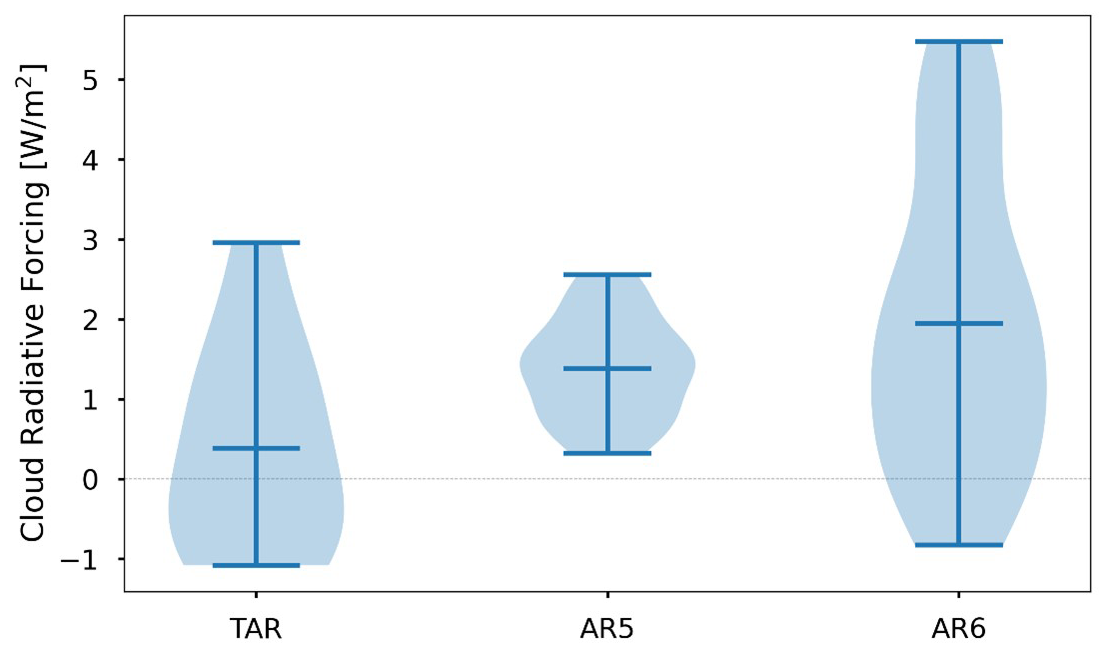
Figure 3 Changes in the distribution of estimated cloud radiative forcing (CRF) across three generations of IPCC Assessment Reports: 3 (TAR, published in 2001), 5 (AR5, 2014), and 6 (AR6, 2021). AR4 is omitted because data necessary to estimate CRF are not readily available. Estimates of simulated CRF were acquired by manual digitization of Fig. 7.2 of Stocker et al. (2001) and by multiplying the equilibrium climate sensitivity and cloud feedback columns from Tables S1 and S2 of Zelinka et al. (2020). As the distribution of estimated cloud radiative forcing shifts upwards from TAR to AR5 to AR6, the figure shows that in AR5 and AR6, cloud feedbacks are largely positive. Indeed, AR6 states with high confidence that “future changes in clouds will, overall, cause additional warming” (Forster et al., 2021, p. 1022), yet it was not clear in TAR whether cloud feedbacks were positive. The increasing confidence in positive cloud feedbacks is partially due to improved boundary layer parameterization, which demonstrates modelers' component-level understanding.

Regarding stratocumulus cloud parameterization in climate models, targeted developments following the Third Intergovernmental Panel on Climate Change (IPCC) Assessment Report reduced uncertainty in estimates of cloud feedbacks to the extent that the Sixth IPCC Assessment Report now states with high confidence that “future changes in clouds will, overall, cause additional warming” (p. 1022). This systematic change in cloud radiative forcing is demonstrated in Fig. 3. It was not clear in the Third IPCC Assessment Report (TAR) whether cloud feedbacks were positive or negative, and the TAR noted in particular that the “difficulty in simulation of observed boundary layer cloud properties is a clear testimony of the still inadequate representation of boundary-layer processes” (Stocker, 2001, p. 273). Around this time, researchers developed improved boundary layer parameterizations with the goal of improving the representation of low boundary layer clouds. For instance, Grenier and Bretherton (2001) built on a standard 1.5-order boundary layer turbulence parameterization in which turbulent mixing is treated as a diffusive process related to the amount of turbulent kinetic energy (TKE) and in which TKE is treated as a conservative, prognostic quantity. Their key additions to the 1.5-order turbulence approach were (1) a more accurate numerical treatment of diffusion in the vicinity of step-function-like jumps in temperature and humidity (inversions) and (2) the contribution of cloud-top radiative cooling to the production of TKE. These two ingredients allow the turbulence parameterization to emulate the physics that drive stratocumulus clouds. Variations on the parameterization of Grenier and Bretherton (2001) and other similarly sophisticated boundary layer parameterizations have been included in numerous weather and climate models, leading to improvements in the simulation of stratocumulus clouds specifically and general improvements in model climatology.

In certain circumstances component-level responsibility for particular model biases can be determined. As an example, the Community Earth System Model 2 (CESM2) was recognized as exhibiting a climate sensitivity that is too large – one that did not appear in standard CMIP simulations. This behavior was discovered in a surprising way. Zhu et al. (2021) showed an instability in the simulation of the Last Glacial Maximum, a much colder period than the present day, using CESM2. This instability did not exist in CESM. By reverting to the original component-level microphysics scheme the model behaved as expected, and erroneous specifications of microphysical particle concentrations were discovered and remedied. More generally, the understanding and observational constraint of ice microphysics is a challenge as demonstrated by the very large variations in ice water path across CMIP models. Using perturbed parameter estimation (PPE; e.g., Eidhammer et al., 2024) can also reveal component-level sensitivities and shortcomings.

We take the above cases from CMIP to indicate that climate scientists aim for component-level understanding of their models, which relates to a standard that climate models be at least somewhat intelligible. Adopting the idea of “intelligibility” from philosopher of science De Regt (2017), we can say that a complex model is intelligible for scientists if they can recognize qualitatively characteristic consequences of the model without performing exact calculations. Intelligibility is facilitated by having models made up of components. In dynamical models, these components typically represent real-world processes, even in cases of empirically based parameterizations. More generally, knowing that a model component plays a particular role in a climate simulation – either representing the process as designed or a role later discovered during model development – is invaluable for reasoning about the behavior, successes, and biases of the GCM as a whole.

The climate modeling community has long strived for component-level understanding and intelligibility. This is especially evident in the work on climate model hierarchies, i.e., a group of models which spans a range of complexity and comprehensiveness (Jeevanjee et al., 2017). Writing nearly 2 decades ago, Issac Held (2005) identified model hierarchies as necessary if we wish to understand both the climate system and complex climate models.

We need a model hierarchy on which to base our understanding, describing how the dynamics change as key sources of complexity are added or subtracted (p. 1609)

…the construction of such hierarchies must, I believe, be a central goal of climate theory in the twenty-first century. There are no alternatives if we want to understand the climate system and our comprehensive climate models. Our understanding will be embedded within these hierarchies. (p. 1610)

Along similar lines, and before the advent of CMIP, Stephen Schneider (1979) wrote that

… the field of climate modeling needs to “fill in the blanks” at each level in the hierarchy of climate models. For only when the effect of adding one change at a time in models of different complexity can be studied, will we have any real hope of understanding cause and effect in the climatic system. (p. 748)

These appeals to climate model hierarchies highlight how component-level understanding is a long-standing goal in climate modeling (see also Katzav and Parker, 2015). This is not to say that component-level understanding automatically translates to understanding all model behaviors. Emergent properties such as equilibrium climate sensitivity (ECS) may elude explanation. Even when components such as cloud parameterizations are appealed to as causally relevant for higher ECS values (e.g., Zelinka et al., 2020), it must be granted that these cloud parameterizations interact with other components and pieces of the overall GCM. That is, GCMs exhibit fuzzy modularity – sub-model behaviors do not add up linearly or in an easy-to-understand way (Lenhard and Winsberg, 2010). So, there may be a more complete explanation detailing how, as a whole, the GCM simulates a higher ECS. Producing a complete explanation may prove elusive, however, to the extent that GCMs are epistemically opaque or have such a high degree of complexity that human minds cannot track all of the relevant information (Humphreys, 2009).⁸ Therefore, we do not regard our three proposed types of understanding as exhaustive – perhaps a component interaction or structural type of understanding ought to be theorized and strived for as well.

However, the examples from earlier in this section show how the goal of component-level understanding is regularly achieved, overall model complexity notwithstanding. Having achieved such understanding, scientists can be more confident that their models have indeed captured some truths about the target systems, and they are thereby justified to increase their confidence in these complex models. In the climate modeling literature, component-level understanding routinely leads to model improvements.

We end this section with a brief discussion distinguishing between component-level and statistical understanding. Overall, our analysis is in the same spirit as that of Knüsel and Baumberger (2020), who argue that data-driven models and dynamical models alike can be understood through manipulating the model so that modelers can qualitatively anticipate model behaviors. However, not all manipulations are equal. Manipulating input data and seeing associated changes in output data does not tell you how the model produces its output. The hierarchy of understanding we propose – instrumental, statistical, and component-level – concerns the degree to which and ways in which a model is intelligible or graspable (Jebeile et al., 2021; Knüsel and Baumberger, 2020). Complex models are intelligible or graspable just in the case that, and to the degree that, their behavior can be qualitatively anticipated or explained (De Regt and Dieks, 2005; Lenhard, 2006). From our perspective, component-level understanding puts scientists into a position to better anticipate and better explain model behavior. In general, statistical understanding can help us answer questions such as “do the input–output relations of the model make sense and, if so, in what way do they make sense?” This is great for finding out whether the model's behavior is consistent with expectations across a variety of cases. This may also involve manipulating input and examining associated changes in output to better anticipate future model behavior (Jebeile et al., 2021; Knüsel and Baumberger, 2020). However, this is distinct from learning why the model behaves the way it does. To answer this distinct question, we need to know how the model is working, which, in turn, involves knowing something about the pieces making up the model. Hence, component-level understanding is called for. This is exactly the type of understanding that we see aimed for, and often grasped, in CMIP experiments.

Component-level understanding often involves a different kind of knowledge related to model architecture and beyond input–output relationships. On the one hand it can demonstrate that you know what role the component is playing in the model – this shows some knowledge of model building. It may also be helpful for answering a wider range of what-if-things-had-been-different questions. Finally, and potentially the clearest benefit of component-level understanding, it can tell one what needs to be fixed in cases of error. This should produce additional trust in the modeling enterprise more generally.⁹

4 Lessons learned: examples of component-level understanding in ML

Component-level understanding is not the privilege solely of dynamic climate modeling. ML models can be built with intelligible components as well, although their components look very different from those in dynamic models. In this section, we offer three examples in which ML researchers are able to acquire component-level understanding of model behaviors by intentionally designing or discovering model components that are interpretable and intelligible.

4.1 Attributing model success with physics-informed machine learning

Our first example involves physics-informed machine learning, i.e., machine learning incorporated with domain knowledge and physical principles (Kashinath et al., 2021). Model success can be attributed to a specific component in a neural net if it is known that said component in the neural net is performing a physically relevant role for a given modeling task.

Beucler et al. (2019, 2021) augment a neural net's architecture via layers which enforce conservation laws that are important for emulating convection (see Fig. 2, panel a). These laws include enthalpy conservation, column-integrated water conservation, and both longwave and shortwave radiation conservation. The conservation laws are enforced “to machine precision” (Beucler et al., 2021). Following Beucler et al. (2019) and because this neural net has a physics-informed architecture, we will use the acronym NNA. NNA is trained on aqua-planet simulation data from the Super-Parameterized Community Atmosphere Model 3.0. NNA's results are compared with those of two other neural nets: one unconstrained by physics (NNU) and another “softly” constrained through a penalization term in the loss function (NNL; see Beucler et al., 2019, for further discussion).

All three NNs are evaluated based on the mean squared errors (MSEs) of their predictions and based on whether their output violates physics conservation laws (physical constraint penalty P, given in units of W² m⁻⁴). While NNU has the highest performance in a baseline climate – i.e., a climate well-represented by the training data – NNA and NNL each outperform NNU in a 4 K warmer climate (see Beucler et al., 2019, Table 1), which is impressive since generalizing into warmer climates is particularly challenging for ML models (Rasp et al., 2018; Li, 2023). These results may indicate that NNU performed better in the baseline climate for the “wrong” reasons. Indeed, NNU heavily violated the physical constraints in both the baseline (P=458 ± 5 × 10² W² m⁻⁴) and the 4 K warmer climate cases (P=3 × 10⁵ ± 1 × 10⁶ W² m⁻⁴). Compare these to the NNA case (baseline: P=7 × 10⁻¹⁰ ± 1 × 10⁻⁹ W² m⁻⁴; 4 K warmer: P=2 × 10⁻⁹ ± 5 × 10⁻⁹ W² m⁻⁴).

Beucler et al. (2021) further show that NNA predicts the total thermodynamic tendency in the enthalpy conservation equation more accurately than the other NNs – “by an amount closely related to how much each NN violates enthalpy conservation” (p. 5). The particular layer in NNA responsible for enthalpy conservation is obviously the explanation for this result. This case therefore exemplifies component-level understanding, which was straightforward because of Beucler et al.'s choice of model design.

It should be noted that both NNA and NNL perform well in the 4 K warmer climate and, more generally, “[e]nforcing constraints, whether in the architecture or the loss function, can systematically reduce the error of variables that appear in the constraints” (Beucler et al., 2021, p. 5). This suggests that, when thinking purely about model performance, physical constraints do not necessarily need to be implemented in the model's architecture. However, compared with NNL, Beucler et al.'s use of NNA facilitates straightforward component-level understanding. The component-level understanding is straightforward because we know that, by virtue of the physics knowledge built into the model's architecture, NNA obeys conservation laws as it is trained and as it is tested. We can draw an analogy with dynamical climate models. NNL is to NNA as bias-corrected GCM simulations are to ones which capture relevant physical processes with high fidelity to begin with. Knowing that a model produces a physically consistent answer for physical reasons is a stronger basis for trust than merely knowing that a model produces physically consistent answers due to post hoc bias correction.

4.2 Explaining model error in a case of Fourier neural operators

Another example involves a recent development in using machine learning to solve partial differential equations: the Fourier neural operator (FNO) pioneered by Li et al. (2021). The innovation of FNO is the application of Fourier transforms to enable CNN-based layers that learn “solution operators” to partial differential equations in a scale-invariant way. Building on Li et al. (2021), Pathak et al. (2022) demonstrated that training an FNO network on output from a numerical weather prediction (NWP) model produced a machine learning model that emulates NWP models with high fidelity and efficiency. A key challenge noted by Pathak et al. (2022), however, was a numerical instability that limited application of the FNO model to forecasts of lengths less than 10 d.

Analysis of the instability ultimately led the group to hypothesize that the instability was due to a specific component of the FNO model: the Fourier transform itself. The problem they identified was that the sine and cosine functions employed in Fourier transforms are the eigenfunctions of the Laplace operator on a doubly periodic, Euclidean geometry, whereas the desired problem (i.e., NWP) is intrinsic to an approximately spherical geometry. In essence, the Earth's poles represent a singularity that Fourier transforms on a latitude–longitude grid are not well-equipped to handle. Bonev et al. (2023) adapt the FNO approach to spherical geometry by utilizing spherical harmonic transforms with the Laplace-operator eigenfunctions for spherical geometries as basis functions in lieu of Fourier transforms. These eigenfunctions, the spherical harmonic functions, smoothly handle the poles as a natural part of their formulation. Bonev et al. (2023) report that the application of spherical harmonic transforms, rather than Fourier transforms, results in a model that is numerically stable up to 1 year.

The application of spherical transformations stabilizes the FNO model. Bonev et al. were able to fix the FNO because they could pinpoint the Fourier transformations, a component of the FNO model, demonstrating scientists' component-level understanding.¹⁰

4.3 GAN dissect for future applications in ML-driven climate science

The final example comes from generative adversarial networks (GANs) in computer vision. Bau et al. (2018) identify particular units (i.e., sets of neurons and/or layers) in a neural net as causally relevant to the generation of particular classes within images such as doors on churches. They demonstrate that these units are actually causally relevant by showing what happens when said units are ablated (essentially setting them to 0).

The example demonstrates component-level understanding because the units in question are manipulated. Components within the architecture of the model are turned on and off and the resultant effects are observed.¹¹ This puts us in a position to say, for example, that “these neurons are responsible for generating images of trees, and we know this because turning more of these neurons on yields an image with more trees (or bigger trees) and vice versa. Moreover, the other aspects of the image are unchanged no matter what we do to these neurons”. Bau et al. (2018) also show that visual artifacts are causally linked to particular units and can be removed using this causal knowledge.

This case is analogous to the study from Gleckler et al. (1995) as described in Sect. 3 above. Recall that the cloud radiative effects from the GCMs were “turned off” (substituted out and replaced with observational data) and the calculations of ocean heat transport improved. Scientists could make sense of model error because they knew that a certain deficiency in GCMs, at the time, involved components of the GCMs responsible for representing clouds. In the same way, Bau et al. (2018) are able to intervene on generations of images by linking units in their model to particular types of image classes and examining what happens to the overall image when these units are manipulated. Note that this is distinct from the closely related method of ablating specific subsets of input data, which is more closely aligned with XAI and can therefore yield statistical understanding (see, e.g., Brenowitz et al., 2020; Park et al., 2022).

While GAN dissect is not typically used in climate science research, GANs are beginning to be adopted for some climate applications (Beroche, 2021; Besombes et al., 2021). Additionally, there are potential future applications such as in atmospheric river detection (Mahesh et al., 2024). In any case, this example demonstrates yet again how component-level understanding is achievable with ML.

5 Discussion and recommendations for practice

In this review and perspective paper we have argued that component-level understanding ought to be strived for in ML-driven climate science. The value of component-level understanding is especially evident in the FNO problem described previously (Sect. 4.2 above). Instrumental understanding allowed the group to identify a performance issue (numerical “issues” in the polar regions) that led to numerical instability. While the group did not employ any XAI – statistical understanding – approaches, it is clear that they would have been of limited value in identifying the underlying cause of the numerical instability, since XAI methods only probe input–output mappings. Ultimately the problem was identified and later solved by applying component-level understanding of the FNO network: knowledge that a component of the network implicitly (and incorrectly) assumed a Euclidean geometry for a problem on a spherical domain.

However, a potential objection is that component-level understanding is unnecessary because XAI methods can simply be evaluated against benchmark metrics. For example, Bommer et al. (2023) propose five metrics to assess XAI methods, focusing especially on the methods' output data (referred to as “explanations”). These include the following.

• Robustness of the explanation is determined given small perturbations to input.

• Faithfulness is determined by comparing the predictions of perturbed input and those of unperturbed input to determine if a feature deemed important by the XAI method does in fact change the network prediction.

• Randomization measures how the explanation changes by perturbing the network weights; similar to the robustness metric, the thinking is that “the explanation of an input x should change if the model changes or if a different class is explained” (Bommer et al., 2023, p. 8).

• Localization measures agreement between the explanation and a user-defined region of interest.

• Complexity is a measure of how concise the highlighted features in an explanation are and assumes that “that an explanation should consist of a few strong features” to aid interpretability (Bommer et al., 2023, p. 10).

Insofar as the metrics are deemed desirable, we agree that such an approach could help establish trust in XAI. However, we view such benchmarks as complementary to, rather than a substitute for, component-level understanding. This is because benchmarks yield a sort of second-order statistical understanding. That is, such metrics are largely focused on aspects of input and output data produced by a given XAI method. They are, in a sense, an XXAI method, an input–output mapping to help make sense of another input–output mapping.

Therefore, our recommendation is that ML-driven climate science strive for component-level understanding. This will aid in evaluating the credibility of model results, in diagnosing model error, and in model development. The clearest path to component-level understanding in ML-driven climate science would likely involve climate scientists building, or helping build, the ML models that are used for their research and implementing physics-based and other background knowledge to whatever extent feasible (Kashinath et al., 2021; Cuomo et al., 2022). Clear standards could also be developed for documenting ML architecture, training procedures, and past analyses, including error diagnoses (O'Loughlin, 2023). Perhaps a model intercomparison project could be developed to systematically evaluate ML behavior across diverse groups of researchers. Lastly, with component-level understanding as a goal to strive for, scientists can better develop hybrid models where both ML and dynamic modeling components are employed.

An increasing range of free or low-cost, high-quality resources are now available to enable researchers who are not (yet) experts in ML to gain a deep and practical level of understanding of modern ML model designs and applications. Some examples of free, high-quality resources include the following.¹²

• Practical Deep Learning for Coders – 1: Getting started (fast.ai): https://course.fast.ai/Lessons/lesson1.html

• Related: GitHub – fastai/fastbook: The fastai book, published as Jupyter Notebooks: https://github.com/fastai/fastbook

• Introduction – Hugging Face NLP Course: https://huggingface.co/learn/nlp-course/chapter1/1

• How Diffusion Models Work – DeepLearning.AI: https://www.deeplearning.ai/short-courses/how-diffusion-models-work/

Back in 2005, Held wrote that climate modeling “must proceed more systematically toward the creation of a hierarchy of lasting value, providing a solid framework within which our understanding of the climate system, and that of future generations, is embedded” (p. 1614). We think there is a parallel need in ML-driven climate science: i.e., to develop systematic standards for the use and evaluation of ML models that aid in our understanding of the climate system. Striving for component-level understanding of ML models is one way to help achieve this.