Interactive coupling of a Greenland ice sheet model in NorESM2

On the backdrop of observed accelerating ice sheet mass loss over the last few decades, there is growing interest in the role of ice sheet changes in global climate projections. In this regard, we have coupled the Norwegian Earth System Model (NorESM) with the Community Ice Sheet Model (CISM) and have produced an initial set of climate projections including an interactive coupling with a dynamic Greenland ice sheet. Our focus in this manuscript is the description of the coupling, the model setup and the initialisation procedure. To illustrate the effect of the coupling, we have further performed one chain of experiments under historical forcing and subsequently under high future greenhouse gas forcing (SSP5-8.5) until 2100 and extended until 2300. We find a limited impact of the dynamical ice sheet changes on the global response of the coupled model under the given forcing and experimental setup when comparing to a standard CMIP6 simulation of NorESM with a fixed ice sheet.

1 Introduction

Ice sheets are regularly discussed and studied in the context of their future sea-level contribution (Seroussi et al., 2020, 2024; Goelzer et al., 2020) and as potential tipping elements in the Earth system (e.g., Pattyn et al., 2018). However, ice sheets are recognised not only as Earth system components that strongly respond to climate changes, but also for their potential to influence climate in turn through interactions with atmosphere, land and ocean (e.g. Vizcaino, 2014). Studying ice sheet – climate interactions therefore requires the ice sheets to be coupled to the other Earth system components. These feedbacks become relevant on long enough timescales, typically centennial to multi-millennial. Relevant large-scale processes that give rise to feedbacks include the influence of a changing ice sheet topography on surface temperature and atmospheric circulation (Merz et al., 2014, 2016), changes in runoff and iceberg fluxes that modify ocean stratification (Martin and Biastoch, 2023) and circulation, and ice sheet expansion or retreat that change the surface albedo and the potential for vegetation, modifying the radiation and surface energy budget (Vizcaíno et al., 2010; Stone and Lunt, 2013).

Given the long timescales on which some of these interactions manifest, modelling climate–ice sheet interactions has until recently been mostly out of reach for high-complexity, high-resolution Coupled Model Intercomparison Project (CMIP) models, with CESM2 and UKESM being the only models that delivered coupled climate-ice sheet simulation results under CMIP6 (Muntjewerf et al., 2021; Smith et al., 2021). A large body of work has also focussed on models of lower complexity and/or lower resolution to advance coupled climate–ice sheet science over the last two decades (e.g., Huybrechts et al., 2002; Ridley et al., 2005; Mikolajewicz et al., 2007; Ganopolski et al., 2010; Goelzer et al., 2011; Roche et al., 2014; Gregory et al., 2020). The challenge inherent in these simulations from the ice sheet perspective is bridging the gap between climate boundary conditions produced at a spatial resolution of up to several degrees to the finer ice sheet scale (typical resolution of only a few km). In addition, climate biases often translate into biases in ice sheet state, which has been mitigated e.g. by use of anomaly methods or ad-hoc corrections (e.g. Goelzer et al., 2012). Improving models to reduce climate biases is a hard effort that often requires intensive model development and interactions across different Earth system components. While these problems are typically reduced with higher resolution, they remain some of the most important challenges when implementing ice sheet dynamics in climate models. A key advance, paving the way to include ice sheets eventually in CMIP-type climate models, was the advent of efficient downscaling procedures (Vizcaíno et al., 2010, 2013, 2014; Sellevold et al., 2019), that produce relatively high-quality surface mass balance (SMB) as ice sheet forcing. These exploit a strong elevation (temperature) dependence of some surface mass and energy balance components, in particular of the melt process, which is why they were first successfully implemented for simulations including the Greenland ice sheet (GrIS). For the significantly colder Antarctic ice sheet at present, the SMB is dominated by the distribution of snowfall, which is notoriously difficult to downscale and hinges on the native resolution of atmospheric dynamics. Another remaining challenge for coupled modelling is how to treat the interaction of ice sheets and ocean for the narrow fjords of Greenland and the ice shelves in Antarctica, that are equally not resolved in global climate models. Furthermore, initialising the climate-ice sheet system is a difficult task due to the specific response timescales of the different systems. There is a strong interest of many modelling groups worldwide to overcome these challenges and to work towards coupled climate–ice sheet simulations leading up to CMIP7. These coupled simulations are supported by a community effort under the Ice Sheet Model Intercomparison Project (ISMIP7).

In this paper, we describe the implementation and first results of GrIS coupling in the Norwegian Earth System Model (NorESM), which builds on a similar development for CESM2 and the Community Ice Sheet Model (CISM, Lipscomb et al., 2019). For a detailed (regional) description of the projection results and comparison between coupled and uncoupled experiments, we refer to Haubner et al. (2025). We describe the model with focus on climate–ice sheet interactions and initialisation (Sect. 2) and the experimental setup (Sect. 3). We show results in section 4 and close with Discussions (Sect. 5) and Conclusions (Sect. 6).

2 Model description

In this section, we describe the coupled modelling framework that is novel to NorESM and consists of climate and ice sheet components, the dynamic coupling between them and the initialisation procedure.

2.1 The Norwegian Earth System model (NorESM)

NorESM is a full-complexity CMIP-type Earth system model (ESM) mainly developed by the Norwegian Climate Centre (NCC) consortium. Here, we discuss the model version NorESM2 (Seland et al., 2020), which contributed to CMIP6 (Eyring et al., 2016) without dynamic ice sheets (NorESM2fixed). We have expanded from this CMIP6 version and included interactive coupling with a dynamic GrIS component (Sect. 2.2). NorESM2 shares many technical features with CESM2 (Danabasoglu et al., 2020) because the fundamental model components for land (CLM), atmosphere (CAM), sea ice (CICE), and land ice (CISM) are the same (Fig. 1). The coupling interface between the ice sheet on the one hand and atmosphere and land models on the other hand is also inherited from and identical to CESM2, using the same elevation-class approach (Sect. 2.3) to provide surface mass and energy balance from the atmosphere (CAM) via the land model (CLM) to the ice sheet model. The ocean model in NorESM2 (BLOM), the ocean biogeochemical component (iHAMOCC) and extended atmospheric chemistry options (in CAM) are distinguishing features and lead to a different climate sensitivity compared to CESM2 – specifically, a lower transient climate response (Seland et al., 2020). In version 2, NorESM (like CESM2) can run with only one interactive ice sheet domain at a time (here Greenland). Implementing an Antarctic ice sheet and paleo ice sheets are subject to future model development.

We have run coupled climate-ice sheet simulations with NorESM2 at two different horizontal resolutions of the atmosphere model, called NorESM2-MM (1° × 1°) and NorESM2-LM (2° × 2° resolution) that have both uncoupled (NorESM2fixed) contributions to CMIP6 to compare to. In the following we focus mainly on the higher resolution version and use the name NorESM2 for NorESM2-MM unless indicated otherwise.

2.2 The Community Ice Sheet Model (CISM)

CISM is a thermodynamically-coupled ice sheet model (Lipscomb et al., 2019), run on a structured grid, that can be used for both coupled (Muntjewerf et al., 2020a, b; Petrini et al., 2025) and standalone applications (Lipscomb et al., 2021; Berdahl et al., 2023; Rahlves et al., 2025).

As the GrIS component in NorESM2, we use CISM at 4 × 4 km horizontal resolution and with 11 unequally spaced vertical levels on a variable-thickness sigma coordinate. The surface layer is 23 % and the lowest layer is 3.6 % of the ice column everywhere, with the absolute thickness (in meters) depending on the local ice thickness. With the solver in use, adding more vertical layers has a limited impact on the ice sheet dynamic representation. The ice sheet domain is laid out on a standard polar stereographic projection and restricted to the main Greenland island. The momentum balance is solved with the higher-order depth integrated viscosity approximation (DIVA) approach (Goldberg, 2011; Robinson et al., 2022) including longitudinal stress transmission in a computationally efficient vertically averaged setup. We use a power-law basal sliding relation

$$\begin{array}{}\text{(1)}& {\mathit{\tau }}_{\mathrm{b}}=C_p\mathrm{|}{u}_{\mathrm{b}}{\mathrm{|}}^{\mathrm{1}/m}\end{array}$$

where τ_b is the basal shear stress, u_b is the sliding speed, m is an exponent, and C_p is a basal friction coefficient that can be calibrated locally (Lipscomb et al., 2021). We calibrate C_p in the initialisation approach described in Sect. 2.4. Bedrock change due to glacial isostatic adjustment is not activated. The basic ice sheet model configuration is similar to the NSF NCAR-CISM contribution to the ISMIP6 (Nowicki et al., 2020) standalone projections (Goelzer et al., 2020).

2.3 Coupled Climate – Ice Sheet interactions

2.3.1 Surface energy balance and surface mass balance

In NorESM2, glacier and ice sheet surfaces are treated as an additional land surface type of the land model CLM. This implies that the surface energy and mass balance are computed by the land model, which passes the surface mass balance (SMB) and ice surface temperature as a forcing to CISM once a year. The ice sheet mask (and the albedo) is changing dynamically with the evolving ice sheet cover. The SMB is calculated as the difference between accumulation (snowfall and refreezing of rainfall and/or previously melted snow within the snowpack) and ice loss from surface melt and sublimation:

$$\begin{array}{}\text{(2)}& \mathrm{SMB}=\mathrm{Snowfall}+\mathrm{Refreezing}-\mathrm{Melt}-\mathrm{Sublimation}.\end{array}$$

The available energy to melt snow and ice is calculated from the sum of net surface radiation, latent and sensible turbulent heat fluxes, and ground heat fluxes at the atmosphere/land interface over glaciated grid cells (Lawrence et al., 2019). Sublimation is defined as a positive quantity, so the process can remove mass from the ice sheet. Snow albedo has an important control on the surface energy balance and is calculated with a multilayer model that accounts for radiation penetration, snow grain metamorphism, and snow impurities (Flanner and Zender, 2005; Flanner et al., 2007; van Kampenhout et al., 2020). The influence of elevation on both surface melt energy and SMB (Hermann et al., 2018; van de Wal et al., 2012) poses a challenge in bridging between the relatively low horizontal resolution in CLM (here 1 or 2°) and the higher CISM horizontal resolution (here 4 × 4 km). This is particularly true at the ice sheet margins, where resolving steep SMB gradients becomes difficult at coarse resolution. CLM addresses this challenge by calculating the SMB at multiple elevation classes (ECs) which allows to account for subgrid-scale elevation variations over glaciated land units (Lipscomb et al., 2013; Vizcaíno et al., 2014; Sellevold et al., 2019; Muntjewerf et al., 2021). To encompass the full range of CISM grid surface elevations while adequately representing subgrid-scale topographic variations, ten ECs are considered with boundaries at 0, 200, 400, 700, 1000, 1300, 1600, 2000, 2500, 3000, and 10 000 m (Muntjewerf et al., 2021; Petrini et al., 2025). The choice of this non-uniform boundary distribution is explained by the larger number of ECs needed to capture the steep lower topography at the ice sheet margins, as opposed to a relatively flat high-elevation terrain in the ice sheet interior (Sellevold et al., 2019). In each EC, surface energy fluxes and their impact on SMB are calculated independently. First, the CLM grid cell near-surface temperature (corresponding to the CLM mean grid cell elevation) is adjusted to the “virtual” elevation in each EC using a uniform lapse rate of −6 °C km⁻¹. The temperature in each EC is then used to calculate EC-specific potential temperature, specific humidity, air density, and surface pressure, assuming vertically uniform relative humidity. The CLM grid cell precipitation does not vary through ECs but is partitioned into snow or rain based on the elevation-corrected near-surface temperature in each EC. If the downscaled temperature is below −2 °C, precipitation is assumed to be 100 % snow, whereas for temperatures above 0 °C it is considered as 100 % rain. For intermediate temperatures between −2 and 0 °C, a linear interpolation is applied to determine the rain-to-snow ratio (Muntjewerf et al., 2021). Snowfall is converted to ice when the depth of the snowpack exceeds a threshold of 10 m water equivalent. For lower snowpack depth, the snow changes are handled by the land model like seasonal snow in other locations and do not enter the ice sheet mass budget. Liquid and solid precipitation and the EC-specific interpolated fields are used to calculate the SMB in each EC. After this calculation, the SMB is downscaled to the higher-resolution CISM domain through a horizontal bilinear interpolation and a linear vertical interpolation between ECs adjacent to the CISM grid cell elevation. Following these interpolations, the discrepancy between total annual mass accumulation and loss in the source (CLM) and destination (CISM) grids is calculated, and two different normalisation factors (one for the accumulation region, and one for the ablation region) are applied to achieve mass conservation. The CLM near-surface temperature is remapped from CLM to CISM using the same EC method, with the only difference being that no normalisation factor is applied after the downscaling. The surface energy and surface mass balance scheme has been extensively tested and evaluated in the framework of CESM2 (van Kampenhout et al., 2020). More details on the coupling between CLM and CISM and on the ECs methods can be found in Muntjewerf et al. (2021) and Sellevold et al. (2019).

In the results section below, we will compare the output of this EC approach implemented in NorESM (NorESM2-EC) over the historical period with two different results from the regional climate model MAR v3.12 (Fettweis et al., 2017). In one case the output is produced by forcing MAR with lateral boundary conditions from the CMIP6 version of NorESM2-MM (NorESM2-MAR). Note that this version of NorESM2 does not include an interactive ice sheet model and represents a different ensemble member with different inter-annual and inter-decadal variability. In the other case, MAR is forced with lateral boundary conditions coming from the reanalysis data set ERA5 (ERA5-MAR).

2.3.2 Ice sheet surface topography

To include the impact of changing ice sheet surface topography on atmospheric circulation, we adopt an asynchronous procedure that modifies the restart files of the atmospheric model (Lofverstrom et al., 2020). Topographic changes on the GrIS domain are interpolated and incorporated in the high-resolution input dataset for the atmospheric component (CAM). Surface topography and surface roughness are then re-calculated and written into the CAM restart file. The procedure is time-consuming and model progress is paused during the update. Including the update at runtime instead would be desirable but requires substantial recoding of the way topography and roughness boundary conditions are currently handled in CAM. In the present experiments we update the topography every five years, in line with the restart checkpoint frequency in our model runs and with earlier experiments with CESM2 (Muntjewerf et al., 2021). For low climate change scenarios and slower ice sheet topography changes, the update frequency could probably be reduced. Such changes should be tested by the user with appropriate control experiments.

2.3.3 Melt and freshwater fluxes

As described above, the ice sheet surface is treated as an additional surface type in the land model, and surface mass and energy calculations are handled by CLM. Surface meltwater runoff is consequently also handled by CLM and routed to the ocean through the runoff scheme (MOSART). This liquid runoff is coupled on hourly timescales at the time resolution of the land model. Ice sheet calving fluxes (i.e., solid ice discharge) are converted to freshwater and passed directly to the ocean, where the energy needed to melt ice is taken from the ocean heat reservoir. Solid ice fluxes are accumulated, passed to the ocean annually, and homogeneously distributed within the year.

2.3.4 Ice–ocean interactions

Our model does not include direct effects of the ocean on the ice sheet (e.g., via ocean temperature or salinity). Also, the ice sheet model is restricted to simulating grounded ice, with all floating ice removed immediately. The spatial scale of narrow marine-terminating outlet glaciers around Greenland is on the order of only a few kilometres, while a typical horizontal resolution of the ocean model is on the order of 100 km (here at 1° × 1°). Resolving their interactions is therefore challenging. Complex interactions between the outflowing glacial meltwater, inflowing ocean water, sea-ice and icebergs and variations in local bathymetry and glacier geometry in ∼ 200 individual fjords complicate the situation. Feasible approaches are currently mostly found in simple parameterisations describing the impact of the ocean on the ice sheet (e.g., Slater et al., 2019, 2020). In the absence of dedicated oceanic forcing of the marine-terminating outlet glaciers in our model, glaciers are simulated to respond passively to changes in inland inflow and SMB and deliver excess mass to the ocean (e.g. Muntjewerf et al., 2020a, b).

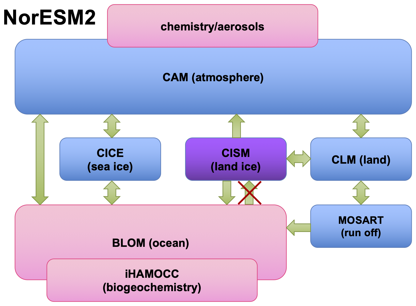
Figure 1 NorESM2 model components and their interactions. Single- and double-headed arrows indicate one-way and two-way interactions, respectively. Oceanic influence on marine-terminating Greenland outlet glaciers is currently not implemented.

2.4 Initialisation

The aim of our initialisation approach is to produce a pre-industrial coupled model configuration (for simplicity represented by year 1850), that is close to steady state for the climate and ice sheet components. In this first coupled setup with NorESM2, we achieve that by initialising the ice sheet as close as possible to the observed present-day configuration, under SMB forcing derived from a pre-industrial simulation of NorESM2 without ice sheet coupling (NorESM2fixed). The arguments for admitting this slight inconsistency (pre-industrial forcing vs present-day ice sheet configuration) are that (i) we do not know the precise ice sheet geometry before the start of routine satellite observations in ∼ 1990, (ii) differences between the pre-industrial and present-day ice sheet are likely small compared to what can be resolved by the atmospheric component and (iii) the climate components in NorESM2fixed have had the present-day ice sheet geometry as topographic boundary condition in all experiments, including the pre-industrial. Furthermore, this approach facilitates the setup and reduces the preparation time of the coupled model, as it can be used with the tuning of an existing NorESM2fixed configuration from CMIP6. The model infrastructure in terms of ice sheet interactions of NorESM2 is largely identical to CESM2; the main differences are the initialisation modeling choices.

2.4.1 Ice sheet model initialisation

For the coupled experiments, our method leans on our experience with standalone ice sheet simulations (e.g., Goelzer et al., 2020; Rahlves et al., 2025) and attempts to minimise the initial drift arising from introducing the ice sheet component into the global model. To that end we have calibrated the spatially varying basal friction coefficient C_p (see Eq. 1) in the ice sheet model (Lipscomb et al., 2021) to closely reproduce the present-day observed ice sheet elevation when forced with output from NorESM2fixed over the pre-industrial period (see Fig. S1 in the Supplement). We also use three options implemented in CISM that control the behaviour of ice at the margins: (1) an option to remove ice caps and glaciers in the periphery that are not connected to the main ice sheet (option “remove_ice_caps”); (2) Ice is not allowed to form in locations disconnected from the main ice sheet (option “block_inception”). This means that new ice sheet cells can only form by flow from an already existing cell; (3) the ice sheet is constrained by masking to the observed ice extent, allowing for retreat but not expansion of the ice sheet area beyond the present-day margins (option “force_retreat” with constant mask). In all three cases, ice thickness is set to zero and ice mass is removed as calving flux. CESM2 experiments used option “remove_ice_caps” and “block_inception” (Muntjewerf et al., 2020a, b), but not the most constraining “force_retreat”. These constraints are justified for forcing scenarios where we expect an ice sheet extent similar or retreated compared to today (historical and future periods). In other cases, e.g. glacial periods, this approach should be modified.

In combination, masking and calibration of the basal friction coefficients are means to practically deal with the climatic biases in NorESM2 and the limitations of the ice sheet model. The dynamic behaviour of the model is somewhat impacted by these choices (e.g., Berends et al., 2023), but the result is an overall better agreement with the ice sheet surface elevation to which the climate model is already relaxed (Fig. 2).

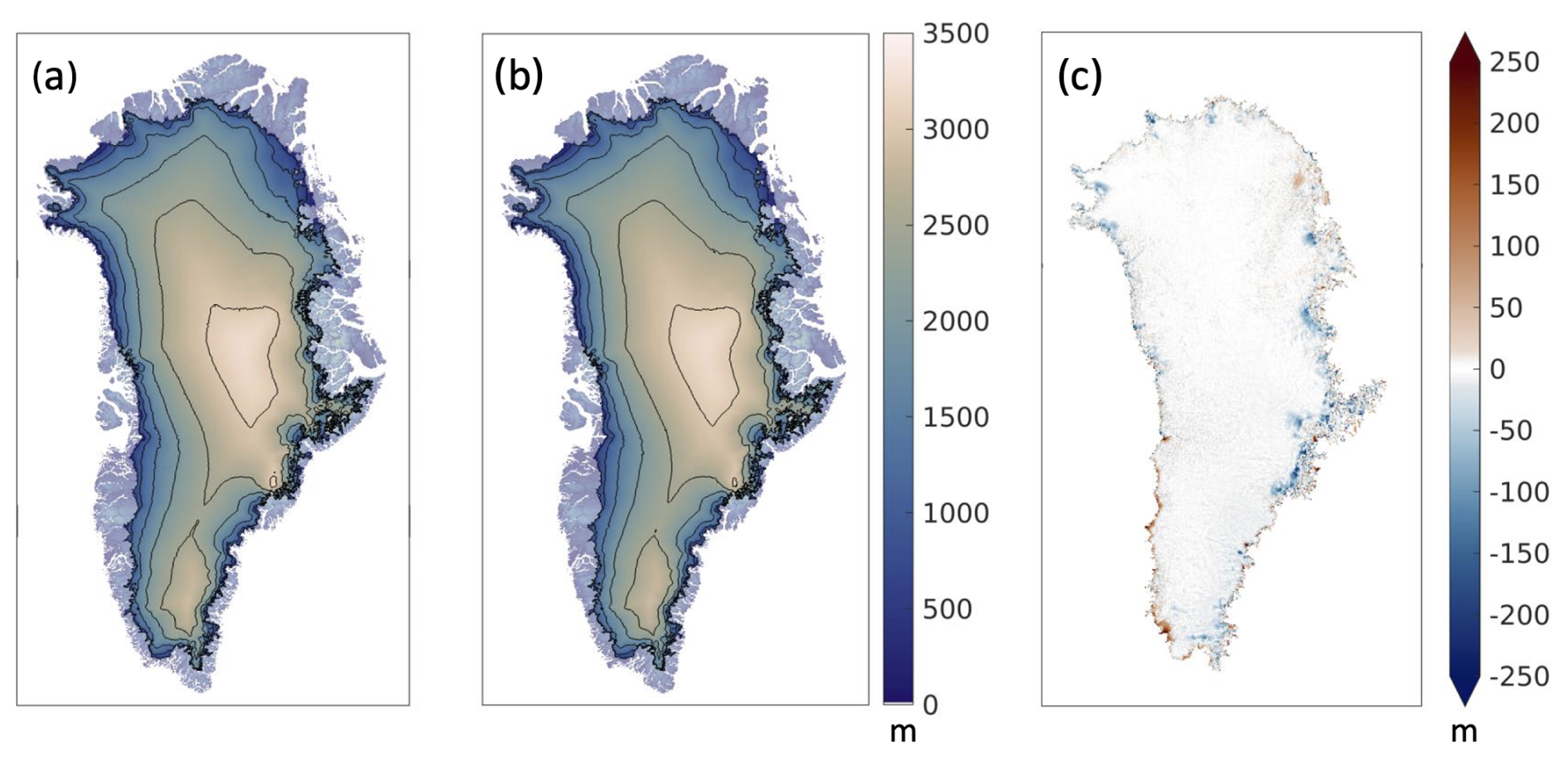
Figure 2 Ice sheet surface elevation. (a) Target surface elevation based on present-day observations (Morlighem et al., 2017). (b) Ice sheet model surface elevation after initialisation for year 1850. (c) Difference in surface elevation on the modelled ice mask.

2.4.2 Coupled model initialisation

The desired consequence of the modelling decisions described in the last section is to minimise model drift and rapidly reach a quasi-equilibrium for the coupled system with an ice sheet geometry close to observed. It has allowed us to perform coupled simulations with very limited model drift after a short relaxation of only 50 years (c1850 in Table 1). This is a strong benefit over other approaches that require relatively expensive iterations to bring the ice sheet and climate states into agreement (e.g., Fyke et al., 2014; Lofverstrom et al., 2020; Muntjewerf et al., 2020a, b). A slight increase in precipitation over Greenland margins in response to the coupling observed during preliminary tests was further compensated by initialising the ice sheet to a slightly biased surface mass balance forcing. Instead of calculating the long-term mean SMB from the last 50 years of a pre-industrial steady state experiment of NorESM2fixed, we use only the 25 years with the highest SMB for the improved initialisation. As opposed to a slight mass gain in the preliminary forward experiment, the result is a small overall ice sheet mass loss, as the ice sheet relaxes to the ensuing lower SMB in the forward experiment (Fig. 3d). The effect of the three masking options described above is illustrated in Figs. S2 and S3.

3 Experimental setup

We have performed one chain of experiments (Table 1) that follow a subset of the protocol for coupled climate–ice sheet simulations (Nowicki et al., 2016) of the Ice Sheet Model Intercomparison Project for CMIP6 (ISMIP6). The first coupled experiment (c1850) is a 50-year relaxation in which the climate and ice sheet are first brought together after separate initialisation. Following is a standard historical experiment (cHIST) from 1850–2014, and a projection under forcing scenario SSP5-8.5 to 2100 (cSSP585), that is further prolonged with a scenarioMIP extension (O'Neill et al., 2016) for SSP5-8.5 to 2300 (cSSP585Ext). We also performed a control experiment continuing the standard CMIP6 pre-industrial experiment for 350 years (cControl). For all coupled experiments, we compare to results from uncoupled experiments (NorESM2fixed, climate simulations indicated with “n”, Table 1) to evaluate the impact of the coupling, albeit with only one ensemble member per model setup.

Table 1 Experiment overview.

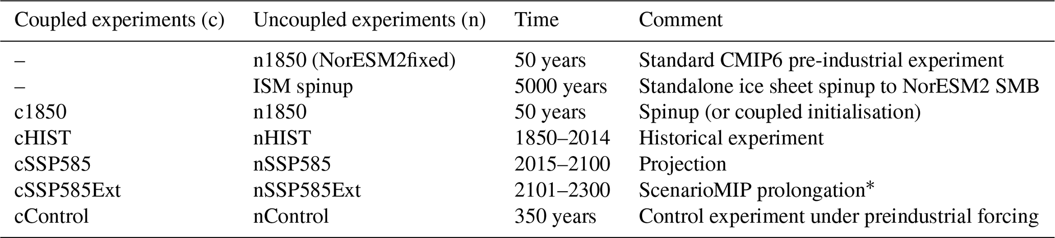
^* SSP585Ext extends SSP585 to year 2300 with CO₂ emissions that are reduced linearly starting from 35 Gt yr⁻¹ in 2100 to less than 10 GtC yr⁻¹ in 2250 and constant during the last 50 years. Other emissions are held constant at 2100 levels.

4 Results

4.1 Simulation over the historical period

Over the historical period, coupled and uncoupled experiments show overall a similar mean climate evolution (Fig. 3a–c). There are differences between the phasing of their interannual and inter-decadal variability, but this is to be expected in freely evolving (i.e., not nudged to observations) ESM simulations. The ice sheet exhibits a small mass loss (positive sea-level contribution) of similar magnitude in the historical experiment cHIST and the control experiment cControl (Fig. 3d), as a result of the initialisation to slightly biased SMB forcing described above (Sect. 2.4.2). The overall mass loss rate over the historical period is comparable to reconstructions (Zuo and Oerlemans, 1997; Box and Colgan, 2013), while episodes of readvance and retreat suggested e.g. by Bjørk et al. (2012) are not captured. In line with the overall mass loss over the historical period, the ice sheet surface elevation slightly decreases, but remains in close agreement with observations used as an initialisation target in 1850 (see Fig. S4). Surface velocities are also close to the observed even though they are not explicitly calibrated for (see Fig. S5).

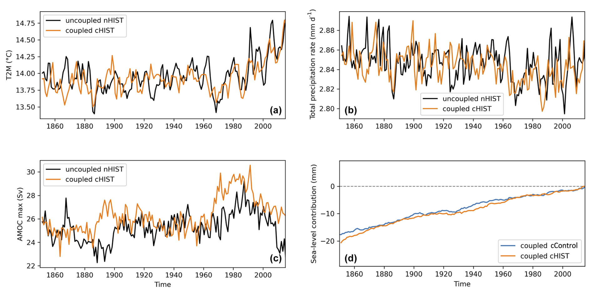
Figure 3 Climate and ice sheet evolution over the historical period. Coupled (orange) and uncoupled (black) evolution of (a) global mean two-meter air temperature (T2M), (b) global mean total precipitation rate (c) Atlantic meridional overturning circulation (AMOC). (d) sea-level contribution from the GrIS for coupled experiments cHIST (orange) and cControl (blue).

4.2 SMB evaluation over the reanalysis period

Figure 4 shows the mean SMB over the period 1960–1989 as simulated directly by NorESM2-EC (Fig. 4a, i.e., NorESM with elevation classes to downscale the SMB within the model) compared to a dynamically downscaled SMB with the regional model MAR (Fig. 4b, NorESM2-MAR). This is further compared to the SMB as obtained by MAR when forced by the ERA5-observational product for the same period (Fig. 4c, ERA5-MAR), which can be seen as our observation-based target. While NorESM2 by itself (NorESM2-EC) captures the main features (north-south gradient, high SMB in the south-east, negative SMB in the central west), the dynamically downscaled products show considerably more detail and larger areas of negative SMB around the margins. Strong similarity between the two MAR products indicates that the dynamical downscaling has a larger impact on the results than the global boundary condition (NorESM2-MAR vs ERA5-MAR).

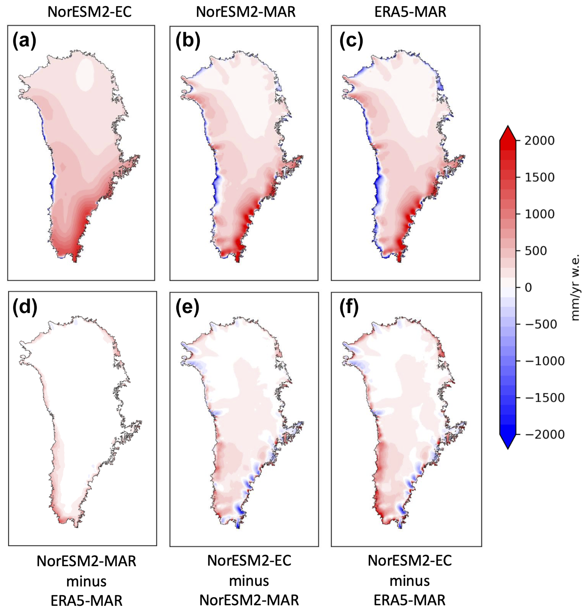
Figure 4 Mean surface mass balance (SMB) over the period 1960–1989 from (a) NorESM2-EC, (b) NorESM2-MAR and (c) ERA5-MAR and differences (d–f). All three fields are masked to the modelled ice sheet area in NorESM2 at the end of year 2014.

Comparing the mean 1960–1989 SMB of NorESM2 with dynamically downscaled products NorESM2-MAR and ERA5-MAR shows that precipitation is smoothed out into the interior in the south-east, and topographically driven precipitation is generally not well resolved due to the relatively coarse resolution of the atmosphere model. A comparison with NorESM2-LM with a 2° horizontal resolution in the atmosphere illustrates these biases further (see Fig. S6). SMB around the margins is generally too high, which can partly be explained by a cold bias of the simulated near-surface temperatures over GrIS margins (Fig. 5) compared to ERA5 (Hersbach et al., 2020) and also present in NorESM2fixed (cf. Seland et al., 2020). Although the averaged summer temperature (JJA) shows a warm bias over most of the ice sheet, a narrow band of colder temperatures prevails over most of the ice sheet margins (Fig. S7). In addition, there is a positive precipitation bias over most of the ice sheet and particularly over southern Greenland (Fig. 6). This result is also supported by the difference between NorESM2-MAR and ERA5-MAR (Fig. 4d), indicating that even after downscaling the SMB is biased high in NorESM2-MAR compared to the reanalysis-driven run.

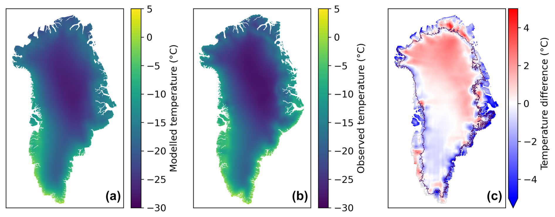
Figure 5 Annual mean 2 m air temperature for the period 1981–2010 in NorESM2 (a) compared to ERA5 (b) and differences (c). The black contour in (c) marks the ice sheet extent.

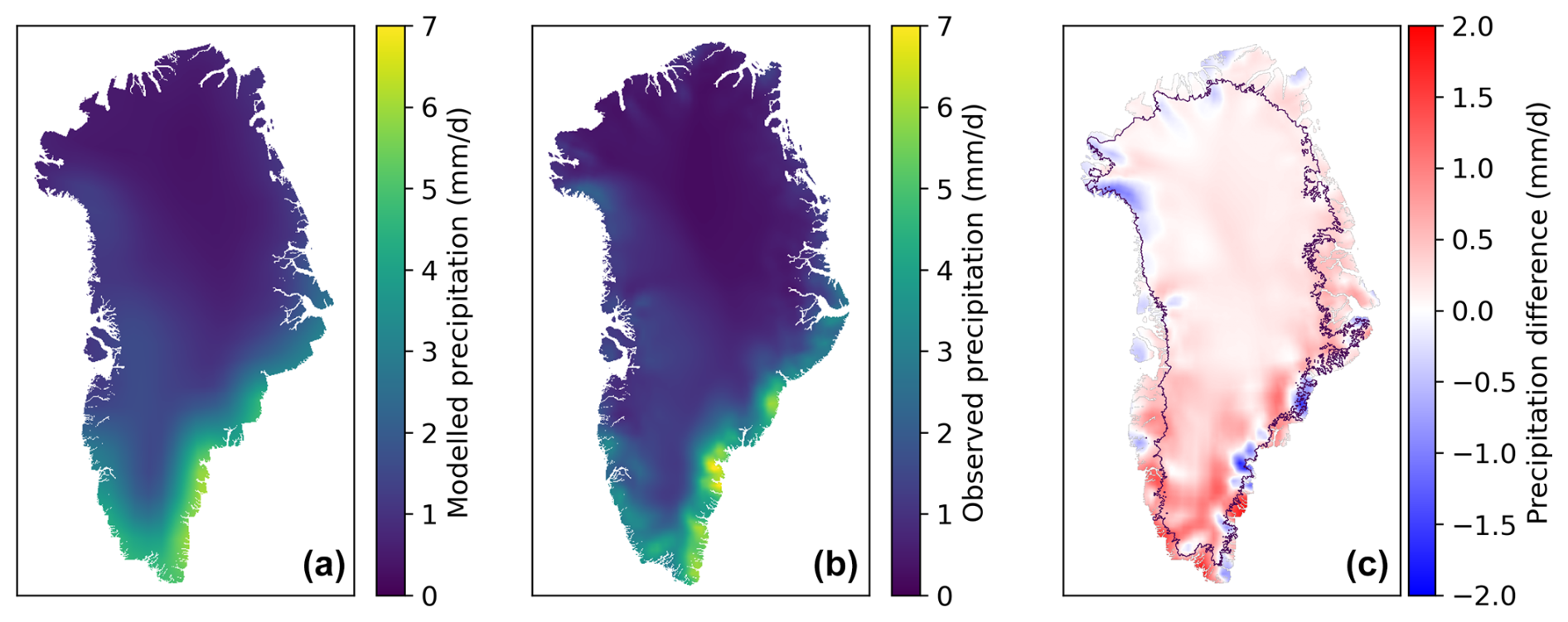
Figure 6 Average annual precipitation rate for the period 1981–2010 in NorESM2 (a) compared to ERA5 (b) and differences (c). The black contour in (c) marks the ice sheet extent.

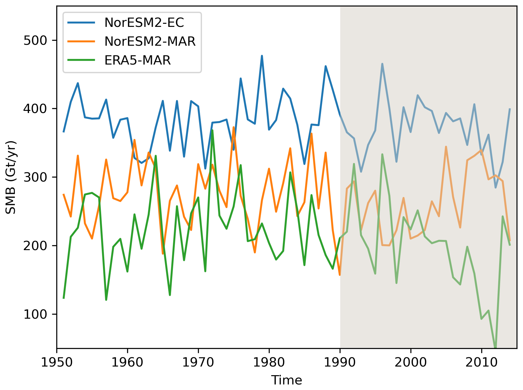
Figure 7 Historical total surface mass balance (SMB) variations integrated over the modelled ice sheet area. The grey shaded area indicates the period 1990–2014 over which SMB trends are calculated and discussed in the main text.

Due to the biases described above, the spatially integrated SMB is higher in NorESM2 (380 Gt yr⁻¹) compared to both NorESM2-MAR (284 Gt yr⁻¹) and ERA5-MAR (230 Gt yr⁻¹) (Fig. 7). Comparison between NorESM2-EC and NorESM2-MAR shows that the NorESM2 version used for downscaling with MAR is a different ensemble member with a different inter-annual and inter-decadal variability. This illustrates that direct comparison on inter-annual and even multi-decadal time scales of individual ensemble members with observations is problematic. That also applies to SMB trends after 1990 that are negative in NorESM2-EC and seemingly of the right sign when compared with ERA5-MAR, albeit with a muted response (−1.2 Gt yr⁻¹ vs. −5.3 Gt yr⁻¹). Comparison with NorESM2-MAR with a positive SMB trend (4.0 Gt yr⁻¹) however clearly shows that the inter-annual/ inter-decadal variability in the ESM is not aligned with observations/reanalysis and can have considerable mismatch over these time intervals. The SMB trends after 2000 show increasing amplitude (both positive and negative) with −6.1 (7.9) [−8.9 Gt yr⁻¹] for NorESM2 (NorESM2-MAR) [ERA5-MAR].

The SMB variance over the period 1960–1989 in NorESM2 (1750 Gt yr⁻¹) is lower compared to NorESM2-MAR (2185 Gt yr⁻¹) and much lower compared to ERA5-MAR (2915 Gt yr⁻¹), which we attribute to an under-developed ablation area in NorESM2 that prohibits inter-annual temperature variations to fully translate to variations in melt and runoff. The Greenland cold bias in NorESM2 can explain the difference in variance between NorESM2-MAR and ERA5-MAR in a similar way.

4.3 Future projection

Global mean temperature increases by ∼ 3.5 °C between 2014 and 2100 and by ∼ 10 °C in 2300 under SSP5-8.5 and extended forcing (Fig. 8a). Northern Hemisphere sea-ice extent dramatically decreases as a result (Fig. 8b), with the minimum extent reaching zero (sea-ice free summer Arctic) by the beginning of the 22st century and a maximum extent approaching zero by the beginning of the 23rd century (practically sea-ice free Arctic year-round). The Atlantic Meridional Overturning Circulation (AMOC) shows a decline already at the end of the historical experiment, which continues over the 21st and 22nd century to a near complete shutdown state at the end of the 23rd century (Fig. 8c).

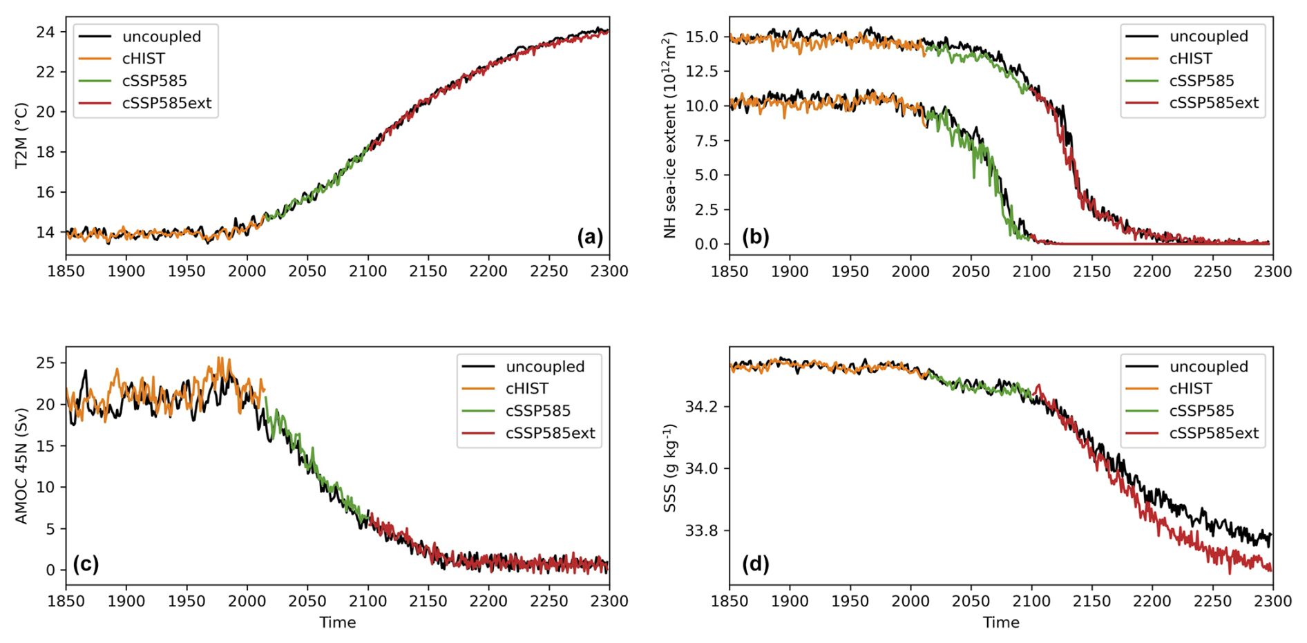
Figure 8 Large-scale climate characteristics for NorESM2 (colour) compared to NorESM2fixed (black). (a) global mean 2 m air temperature, (b) maximum and minimum northern hemisphere sea-ice extent, (c) AMOC strength at 45° N, (d) global mean sea surface salinity.

Most global climate characteristics show similar behaviour in the coupled and uncoupled experiments, indicating that the interactive ice sheet coupling has limited effect on the large-scale climate behaviour in our model under the given forcing. In particular, the evolution of the AMOC is hardly affected by the additional freshwater flux from GrIS mass loss in the coupled experiment (cf. Fig. 9a and b), which amounts to 0.004, 0.052 and 0.113 Sv averaged over the 21st, 22nd and 23rd century, respectively. The only global variable where differences are clearly visible is global sea surface salinity that is reduced in the coupled model compared to NorESM2fixed (Fig. 8d) in response to that additional freshwater input. A detailed analysis of the (regional) differences between the coupled NorESM2 and the version with fixed ice sheets NorESM2fixed can be found in Haubner et al. (2025).

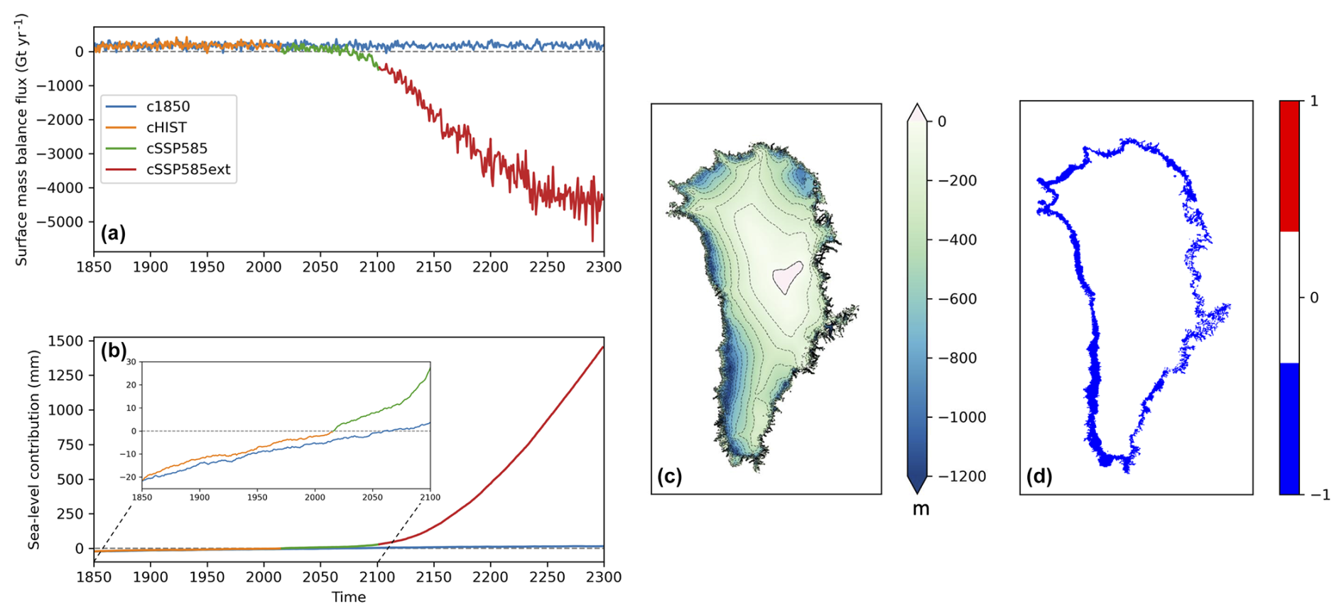
Figure 9 GrIS characteristics for the chain of experiments: (a) total surface mass balance, (b) sea-level contribution, (c) ice thickness change and (d) ice mask change between 2014 and 2300 (blue indicating retreat).

Increased mass loss of the GrIS compared to the historical background trend first emerges at the beginning of the projection period ∼ 2015–2025 (Fig. 9b). However, instead of further accelerating ice sheet retreat after 2025, as might be expected from the global temperature evolution, we see a nearly constant rate of mass loss until 2080. This can be explained by a rapidly weakening AMOC, which leads to regional cooling in the North Atlantic that offsets a substantial part of the warming trend. Compared to results based on standalone ice sheet simulations over the same period with a large range of models (Goelzer et al., 2020), the projected sea-level contribution in NorESM2 is below the lower bound, which we attribute to both the strong AMOC response and an initial cold bias of NorESM2. However, a similar experiment with CESM2-CISM (Muntjewerf et al., 2020b) shows a strongly decreasing SMB already after 2050, despite a decreasing AMOC, which may be explained by a different ocean model or different interdecadal variability between the two global models.

The mass loss rate increases towards the end of the 21st century and continues to do so until the end of our experiment in year 2300. The surface mass balance over the extension period is rapidly decreasing and leads to a cumulated sea-level contribution of close to 1.5 m by 2300 (Fig. 9a–b). The ice sheet loses mass, thins by more than 1 km mainly around the coast, and exhibits retreat of several tens of km around the entire margin (Fig. 9c–d).

5 Discussion

The presented model development and experiments represent the first interactive coupling of the GrIS in the global Earth System Model NorESM. This work shines light on challenges that are inherent to combining model components of different spatial resolution.

Climate model biases due to limited resolution of the atmospheric component are difficult to overcome, given that current global climate models are typically run at the upper limit of available High Performance Computing resources. While the elevation-class approach for downscaling is successful for SMB and surface energy components with strong temperature dependence, improving the distribution of mostly topographically controlled precipitation is very difficult. In this context, the potential of regional grid refinement is promising, a possibility that emerges with the CAM spectral element dynamical core (van Kampenhout et al., 2019; Herrington et al., 2022) that is available in the next version of our model, NorESM3. Another important new capability of NorESM3 is a flexible framework for employing different data model components, which already plays an important role in our ongoing development work.

NorESM2 has been initialised and run with a dynamic GrIS in a complementary way compared to the approach taken with CESM2 (Muntjewerf et al., 2020a, b). Compared to these studies, we have tried to initialise closer to the observed ice sheet geometry and mitigate model drift by using stronger constraints on the ice sheet model. The approach of nudging the ice sheet thickness toward observed values during initialisation by calibrating the basal friction coefficients is very effective but also has its caveats. Inaccuracies in model physics, parametrisations and boundary conditions are compounded into a modified basal friction field with effects that are hard to trace. In particular, any bias in the SMB (which we know can be substantial in some regions) is propagated into the dynamic behaviour of the ice sheet model in a non-transparent way (Berends et al., 2023). Masking the ice sheet to the observed present-day ice extent is also a strong limitation to the ice sheet physics and is only justified for the strong warming scenario applied here, where the entire ice sheet margin retreats. It remains a challenge to reduce the impact of climate and ice sheet biases (which are often mutually reinforcing) on the coupled state while maintaining the full prognostic capabilities of the model. Efforts to include ice sheet components in Earth system models are underway in various groups around the world and are supported by ISMIP7 and other intercomparison exercises. This opens possibilities for collaboration and exchange to tackle outstanding issues together.

The assumption that the pre-industrial ice sheet state is close to the present-day observed one is questionable and could be refined e.g. by running one or several iterations from pre-industrial to 1990 with an updated 1850 state to better match the transient historical ice sheet state. However, such a refinement would add many more model years to the experimental setup, and its success could be dependent on controlling internal variability of the system. More reconstructions of the climate and ice sheet states further back in time, ideally towards the pre-industrial climate, would be very useful in this context (e.g. Kjær et al., 2012; Bjørk et al., 2012).

Since we have focused on describing the ice sheet coupling, we have not analysed the climate evolution over the historical and future period in great detail. A deeper analysis of differences between the coupled and uncoupled experiments can be found in a separate paper (Haubner et al., 2025). However, it is apparent that the influence of ice sheet changes on the global mean climate is rather limited in the current setup and for the given forcing. In particular, we may have expected a larger response of the AMOC to the additional freshwater input coming from Greenland, even if the lack of a dedicated ocean forcing in our setup may be under-estimating ice sheet retreat to some extent. It appears that the AMOC weakening in the model version without ice sheet coupling is already so intense in NorESM2 (Schwinger et al., 2022), that the freshening due to ice sheet meltwater fluxes has little additional effect.

6 Conclusions

This paper describes the first coupled climate–Greenland ice sheet model setup of NorESM and illustrates its behaviour with first simulation results. We have presented modelling choices which are effective in working around some of the climate biases and in preparing a present-day ice sheet state that is close to observations. The simulated present-day surface mass balance in NorESM captures the main features when compared to high-fidelity regional climate model simulations but does not represent the detailed distribution of precipitation very well due to the relatively coarse resolution of the atmosphere. Experiments under a strong future warming scenario until 2300 show a limited effect of including the Greenland coupling on most global variables under the given forcing.

Other challenges of coupling Earth system components of different typical response timescales and spatial resolution remain. Further work with NorESM is therefore ongoing, e.g. to include the coupling of marine-terminating outlet glaciers with the ocean, and to improve the representation of SMB over the GrIS. We are also working towards coupling with the Antarctic ice sheet, which is an obvious next step but includes additional challenges, in particular a less effective downscaling of SMB boundary conditions due to a limited contribution of melt and the important interaction between ice shelves and the Southern Ocean.