Improving the representation of major Indian crops in the Community Land Model version 5.0 (CLM5) using site-scale crop data

Accurate representation of croplands is essential for simulating terrestrial water, energy, and carbon fluxes over India because croplands constitute more than 50 % of the Indian land mass. Wheat and rice are the two major crops grown in India, covering more than 80 % of the agricultural land. The Community Land Model version 5 (CLM5) has significant errors in simulating the crop phenology, yield, and growing season lengths due to errors in the parameterizations of the crop module, leading to errors in carbon, water, and energy fluxes over these croplands. Our study aimed to improve the representation of wheat and rice crops in CLM5. Unfortunately, the crop data necessary to calibrate and evaluate the models over the Indian region are not readily available. This study used comprehensive wheat and rice novel crop data for India created by digitizing historical observations. This dataset is the first of its kind, covering 50 years and over 20 sites of crop growth data across tropical regions, where data have traditionally been spatially and temporally sparse. We used eight wheat sites and eight rice sites from the recent decades. Many sites have multiple growing seasons, taking the total up to nearly 20 growing seasons for each crop. We used these data to calibrate and improve the representation of the sowing dates, growing season, growth parameters, and base temperature in CLM5. The modified CLM5 performed much better than the default model in simulating the crop phenology, yield, and carbon, water, and energy fluxes compared to site-scale data and remote sensing observations. For instance, Pearson's r for monthly leaf area index (LAI) improved from 0.35 to 0.92, and monthly gross primary production (GPP) improved from −0.46 to 0.79 compared to Moderate Resolution Imaging Spectroradiometer (MODIS) monthly data. The r value of the monthly sensible and latent heat fluxes improved from 0.76 and 0.52 to 0.9 and 0.88, respectively. Moreover, because of the corrected representation of the growing seasons, the seasonality of the simulated irrigation matched the observations. This study demonstrates that global land models must use region-specific parameters rather than global parameters for accurately simulating vegetation processes and corresponding land surface processes. The improved CLM5 can be used to investigate the changes in growing season lengths, water use efficiency, and climate impacting crop growth of Indian crops in future scenarios. The model can also help provide estimates of crop productivity and net carbon capture abilities of agroecosystems in future climate.

1 Introduction

Land surface models (LSMs), the land components of Earth system models (ESMs), represent a wide variety of processes, including energy partitioning, carbon and mass exchange, and interaction with the hydrological cycle, to name a few. LSMs provide boundary conditions and interact with various components of ESMs (Fisher and Koven, 2020; Strebel et al., 2022). LSMs have come a long way, from a very basic representation of the energy budget at the surface level to a very complex state where each grid cell consists of multiple land units and a unique interaction of the individual land unit with the atmospheric forcings (Blyth et al., 2021; Ruiz-Vásquez et al., 2023). LSMs use sophisticated parameterization and modules to represent complex land surfaces and their interactions with other components of ESMs. One important component of LSMs that significantly impacts not only land processes but also atmospheric processes is agricultural land. LSMs strive towards a realistic depiction of agricultural land cover and its processes. Until the last decade, the depiction of crops was mainly constrained to rudimentary models that do not include agricultural practices such as irrigation and fertilization or simply depicted crops as natural grassland (Elliott et al., 2015; McDermid et al., 2017). Enhancements to crop modules gave LSMs a greater capacity to investigate changes in water and energy cycles from croplands and crop yield in response to climate, environment, land use, and land management variations. Recent studies provide valuable insights for enhancing the accuracy of simulating biogeophysical and biogeochemical processes at both regional and global scales in LSMs (Lobell et al., 2011; Osborne et al., 2015; Sheng et al., 2018; Lombardozzi et al., 2020; Boas et al., 2021; Ma et al., 2023).

The Community Land Model (CLM) has, since version 4.0, included a prognostic crop module based on the Agroecosystem Integrated Biosphere Simulator (Agro-IBIS) (Levis et al., 2012; Lawrence et al., 2018, 2019). This module can simulate the soil–vegetation–atmosphere system, including crop yields. The most recent version of CLM, CLM5, is a leading land surface model with an interactive crop module representing crop management. The module comprises eight crop types that are actively managed: temperate soybean, tropical soybean, temperate corn, tropical corn, spring wheat, cotton, rice, and sugarcane. It also contains irrigated, non-irrigated, and unmanaged crops (Lombardozzi et al., 2020). Currently, CLM5 is the sole land surface model incorporating dynamic spatial patterns of significant crop varieties and their management (Lombardozzi et al., 2020). Although CLM5 showed advancements compared to its previous versions, limited research conducted at the point and regional scales indicates that it may provide poor phenology and yield predictions for specific crops (Chen et al., 2018; Sheng et al., 2018; Boas et al., 2021). The energy and carbon fluxes are highly affected by inaccuracies in crop phenology, particularly concerning the timing of planting and harvesting.

The Indian subcontinent is a significant land mass that significantly affects the Earth system's energy, water, and carbon fluxes. Nearly 50 % of the land cover is used for agriculture in India, and two major cereal crops, wheat and rice, occupy nearly 80 % of the total agricultural land. However, CLM5 simulations of rice and wheat over the Indian subcontinent show large biases in simulating annual crop yield (Lombardozzi et al., 2020). The major growing seasons of wheat and rice are the rabi and kharif seasons, but CLM5 grows wheat and rice in the summer and rabi seasons, respectively. The irrigation patterns simulated by CLM have a bias in seasonality, which Mathur and AchuthaRao (2019) highlighted. Irrigation is an essential feature of the croplands in India, especially during the rabi season (Gahlot et al., 2020) for wheat and in dry regions for rice. Therefore, the bias in irrigation points to the lack of accurate representation of Indian crops.

Gahlot et al. (2020) used an LSM (Integrated Science Assessment Model; ISAM) to investigate the wheat croplands of India. The major drawback of the study was the lack of enough site-scale observations to calibrate and validate the model while covering the broad growing conditions of India. Therefore, in this study, we aim to investigate and improve the representation of major Indian crops – wheat and rice – in the latest version of CLM (CLM5.0). We used site-scale observations from multiple sites to calibrate the parameters essential for the crop module in CLM5 and evaluate the model. The site-scale observations cover various climatic conditions experienced by crops in India, thus making this a robust calibration of an LSM. Further, we aimed to quantify the impacts of realistic representation of Indian crops on various land processes such as irrigation, gross primary production, latent heat, and sensible heat.

The current paper is structured as follows: first, we briefly describe CLM5 and the site-scale data used in this study. Then, we describe the shortcomings of CLM5 in simulating Indian crops, comparing them to the observations. Next, we dive into the need for modifications in CLM5 and the changes made to parameters and the source code of CLM5. The Results section compares our improved model at site and regional scales. We compare the CLM5 simulations against observed leaf area index (LAI), yield, and growing season length at site scale. At the regional scale, we compare against yield, irrigation patterns, LAI, gross primary production (GPP), latent heat flux (LH), and sensible heat flux (SH) observations. Finally, we discuss the impact of the study and the conclusions.

2 Materials and methods

2.1 Community Land Model version 5 (CLM5.0)

CLM5 is the latest version of the land component in the Community Earth System Model (CESM) (Lawrence et al., 2018, 2019). The biogeochemistry mode of CLM5 (CLM5-BGC) is widely used to estimate the water, energy, and carbon fluxes in various climatic zones (Cheng et al., 2021; Denager et al., 2023; Song et al., 2020; Seo and Kim, 2023). The biogeochemistry and crop module of CLM5 (BGC-Crop) is modified in various studies to meet regional constraints, and the resulting impact on various fluxes is analyzed (Boas et al., 2021, 2023; Raczka et al., 2021; Yin et al., 2023). Studies show that incorporating agriculturally managed land cover can improve the general representation of biogeochemical processes (Boas et al., 2021). The CLM5 crop module includes new crop functional types, updated fertilization rates and irrigation triggers, a transient crop management option, and some adjustments to phenological parameters (Lombardozzi et al., 2020).

CLM5 has a better representation of the land surface by using a tile representation. This allows the model to have various land types inside a grid cell. In its latest version, the model supports 79 plant functional types with 32 rainfed and 32 irrigated crop types. The complex representation of the land surface makes CLM5 a better model on various metrics tested by International Land Model Benchmarking (ILAMB) (Collier et al., 2018).

The current study used CLM5 in the data atmosphere mode, i.e., not interacting with the atmosphere. The GSWP3 atmospheric data are used for the simulations. We ran CLM5 at two different spatial resolutions from 2000 to 2014: site-scale simulations to calibrate the crop module and regional simulations to evaluate the calibrated model against remote sensing data and derived surface flux data (Sect. 2.5). The plant functional types of the crops in CLM5 considered in this study are wheat (19: rainfed and 20: irrigated) and rice (61: rainfed and 62: irrigated). The default CLM5 is referred to as CLM5_Def throughout this paper. CLM5_Mod1 and CLM5_Mod2 are the two setups of the model developed in this study, and they are described in detail in Sect. 2.3. The overall methodology and steps followed in this study are depicted as a flowchart (Fig. S1 in the Supplement) and explained in detail in the following sections.

2.1.1 Site-scale simulations

For site-scale simulations, we created domain, surface, and land use time series data for the respective sites (for details on sites, see Sect. 2.2 and Fig. 1). The resolution of the data is 0.1° and has one grid cell with the site at its center. The method used to generate the data is available in the documentation of Reddy et al. (2024). The domain file represents the spatial extent of our simulation. The surface data represent the local soil and surface properties. The land use time series reflects the varying land use and land cover change from 1850 to 2015 at sites. Spin-up at each site is carried out for 200 years in accelerated deposition mode (AD mode) and 400 years in normal mode. The GSWP3 atmospheric data are used for the site-scale simulations.

2.1.2 Regional-scale simulations

For regional-scale simulations, we fixed the domain between 60 and 100° E and between 0 and 40° N (Fig. S2), covering the Indian subcontinent. The domain, surface, and land use time series data are generated for the domain mentioned above with a spatial resolution of 0.5° (files available in Reddy et al., 2024). The spin-up for the regional case is carried out in two stages: 200 years of spin-up in AD mode and 400 years in normal mode. The simulation data at the end of 400 years are used as initial conditions for our regional simulations. The regional simulations are run from 1995 to 2014, and the data from 2000 to 2014 are used for the analysis. The GSWP3 atmospheric data are used as atmospheric forcing for the regional-scale simulations.

2.2 Site-scale crop data

Site-scale data of the type and quality required for calibrating and validating crop models are not readily available in India. This is unfortunate because plenty of data have been collected, but they have never been properly archived. India has invested heavily in agricultural studies and has built nearly 70 agricultural institutes nationwide since the green revolution in the 1960s, with each state having at least one institute dedicated to studying regional crops. Master's and PhD student theses from these institutes, many containing site-scale observations, were recently consolidated and brought into the public domain in the KrishiKosh repository (Veeranjaneyulu, 2014). However, the data are complex to extract from these theses because of the data collection and reporting structure differences followed by various institutes. For this study, we assembled data on wheat and rice in a formatted, machine-readable format that can be downloaded and used for model development. The data are available on the PANGEA repository (Varma et al., 2024). We used the site-scale data (years 2000 to 2014) generated by Varma et al. (2024) to evaluate our CLM5 (Table S1 and Fig. 1).

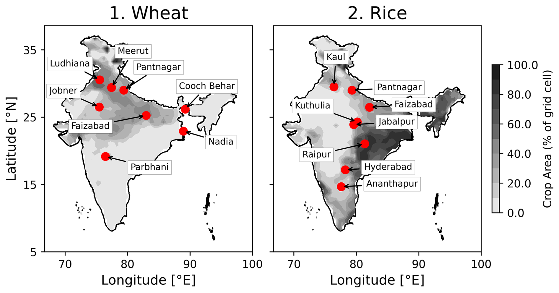
Figure 1 Location of sites used in the current study for calibrating and validating the major Indian crops: (1) wheat and (2) rice. The contour map shows the percent of crop area in each 0.5° grid cell.

2.3 Improvements in CLM5

The parameters impacting planting and growing stages in CLM5 are minimum and maximum planting dates, minimum planting temperature, planting temperature, base temperature for growing degree-day (GDD) calculations, minimum GDD for crop emergence, and GDD threshold for crop grain fill. The minimum planting temperature and the average minimum planting temperature of the growing season govern the planting date of the crop in CLM5. The base temperature defines the crop growth rate and the accumulation of GDDs. Crop growth has different phases: emergence, flowering, grain fill, and maturity. CLM5 simulates the crop growth phases using the accumulated GDDs. Therefore, base temperature becomes a critical parameter that defines the crop growth in CLM5. The base temperature and maximum GDD control the longevity of each phase in crop growth. The allocation to the grain starts once the crop reaches the grain fill stage, which is controlled through the “grnfill” parameter in CLM5. The grnfill parameter defines the threshold for initiating the grain-filling stage as a fraction of the GDDs required for maturity (hybgdd in Table 1). Growing season length in CLM5 is directly controlled through base temperature. The lower the base temperature, the faster the GDD accumulation and the shorter the growing season length. The planting window, base temperature, GDDs required for maturity, and grain fill parameters have a significant impact on crop growth and are considered widely when calibrating the crop module in CLM5 (Fisher et al., 2019; Cheng et al., 2020; Boas et al., 2021).

The improvements to the wheat and rice crops in CLM5 were made in two steps. We first performed a literature survey and conducted sensitivity experiments to find the best-performing parameters shown in Table 1 (Sect. 2.3.1). The CLM5_Mod1 setup is the result of the new parameter values. Second, we calibrated the latitudinal variation in base temperature through sensitivity experiments (Sect. 2.3.2). The CLM5_Mod2 setup results from calibrating the latitudinal variation in base temperature. Changes in the source code of CLM5 were necessary to facilitate the incorporation of changes made to parameters (see Sect. 2.3.1).

2.3.1 Improvements in CLM5_Mod1

Wheat

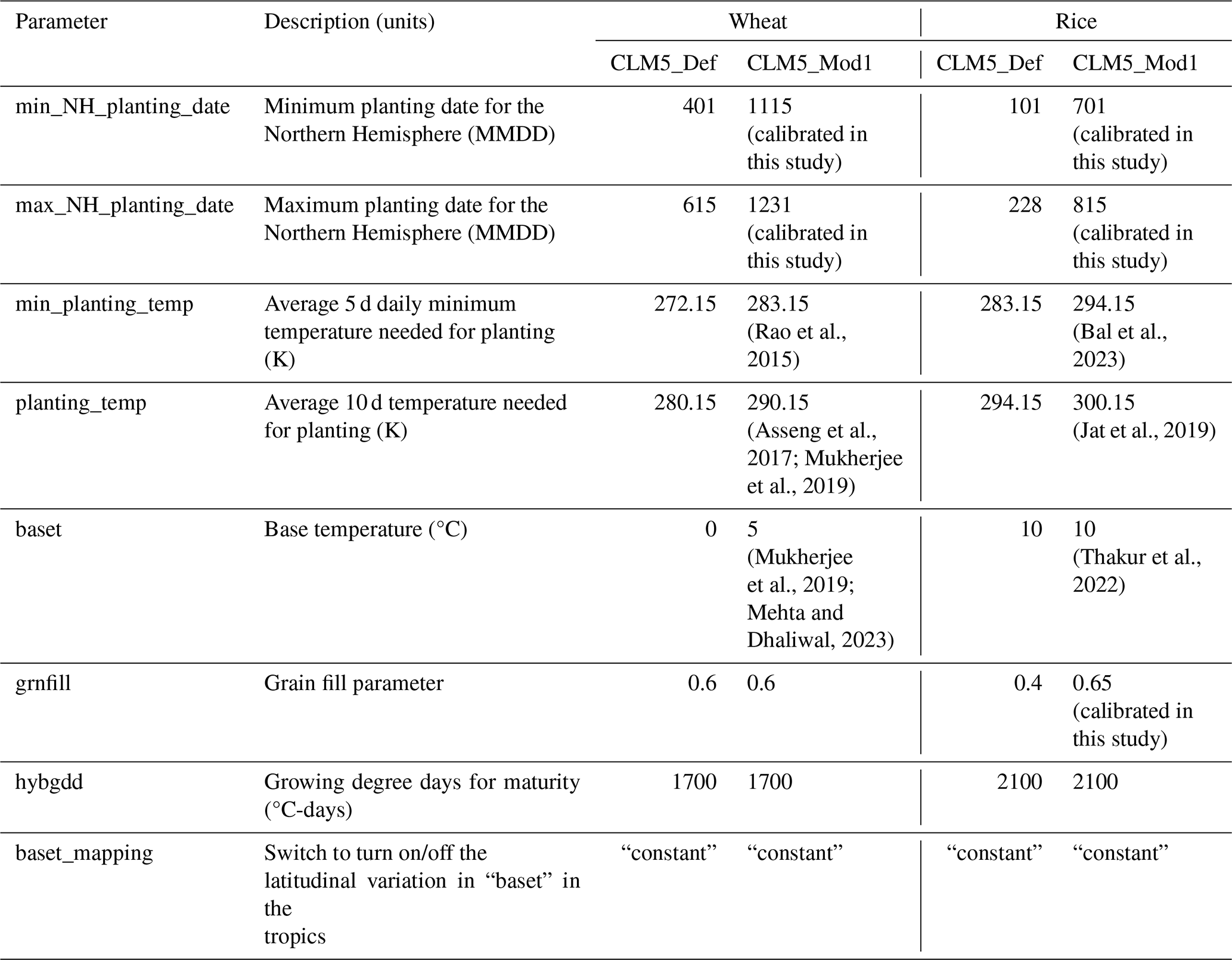
CLM5_Def simulated the wheat growth from April to August. This starkly contrasts with ground reality, where Indian farmers sow wheat in late October to early November and harvest in late March or April (rabi season) (Sacks et al., 2010; Gahlot et al., 2020). To implement a realistic growing season, we performed sensitivity simulations by varying the planting window of 45 d, from mid-October to late November (see Table S2 in the Supplement). The planting window shown in Table 1 produced the best results in lowering the bias in simulated LAI, yield, and growing season length and is therefore used in CLM5_Mod1. The CLM5_Def base temperature for wheat is 0 °C, but during our literature survey, we found that the optimal base temperature for wheat in India is 5 °C (Mukherjee et al., 2019; Mehta and Dhaliwal, 2023). The planting temperature threshold in CLM5 for wheat is low compared to observations in India (Rao et al., 2015; Asseng et al., 2017; Mukherjee et al., 2019). The grain fill threshold of 0.6 for wheat performed well amongst tested values in our sensitivity studies (Table S2), and therefore we did not change the parameter value.

Rice

CLM5_Def simulated rice growth from January to May. In contrast, rice is grown in India during the monsoon season due to the high water requirements of the rice crop. Rice is sown in the last week of June to early July and harvested at the end of October and early November, also known as the kharif season. Many regions in India grow rice during the summer and rabi seasons, which meet their water requirements mainly through irrigation. The rice crop area grown in summer and rabi is very low compared to the rice crop grown in the kharif season (Biemans et al., 2016). Therefore, we confined ourselves to the major rice-growing season (kharif season) to calibrate the model. A sensitivity study was conducted with a planting window of 45 d, from early June to late July (Table S2). The planting window shown in Table 1 for rice gave the best results. The base temperature used for rice crop (10 °C) in CLM5_Def is the same as that observed in the literature for the Indian region (Thakur et al., 2022). However, we found that the planting temperature observed in India differs from those used in CLM5_Def (Jat et al., 2019; Bal et al., 2023). The grain fill threshold used for rice in the CLM5_Def case resulted in very poor LAI and yield simulations, which was recognized earlier by Lu and Yang (2021) while studying rice in China using the CLM. Through a sensitivity test, we found that the grain fill threshold of 0.65 performed the best in simulating LAI and yield for rice amongst the tested grain fill values in Table S2.

The parameter of growing degree days required for maturity (hybgdd) in both wheat and rice performed well during our sensitivity simulations, and therefore its value is not altered. Table 1 shows all the parameters changed in the default CLM5 to improve wheat and rice crop growth for the Indian region.

Table 1 Parameter values for wheat and rice in the CLM5 crop module.

Source code changes

Along with the parameter changes, we had to change the model source code to fix a bug with Northern Hemisphere crop seasons that start in one calendar year and finish in the next. The code added to the module CNPhenologyMod.F90 begins at line 2001 (Sect. S1). The code changes are available in Reddy et al. (2024).

This bug is fixed in more recent versions of the CLM, starting with tag ctsm5.1.dev131. A bug was also fixed to make the CLM use user-specified values of the parameters latvary_intercept and latvary_slope, which allow latitudinal variation of the base temperature. More recent versions of the CLM, starting with tag ctsm5.1.dev155, include this fix.

2.3.2 Mod2 case parameters: varying base temperature by latitude

CLM5 can vary crop functional type (CFT) base temperature by latitude to account for cultivars bred for optimal performance in different climates. Currently, only wheat and sugarcane have these capabilities turned on. We extended this latitudinal variability to rice and improved the existing one for wheat in India. The latitudinal variation in base temperature is defined by two parameters: latvary_intercept and latvary_slope. The equation in the model that uses these parameters is

$$\begin{array}{ll}{\displaystyle }& {\displaystyle }{\text{Tbase}}_{\text{lat}}=\text{Tbase}+{\text{latvary}}_{\text{intercept}}\\ \text{(1)}& {\displaystyle }& {\displaystyle }-min\mathit{\{}{\text{latvary}}_{\text{intercept}},{\text{latvray}}_{\text{slope}}\cdot |\text{latitude}\left|\mathit{\right\}},\end{array}$$

where latvary_slope and latvary_intercept define the latitudinal extent of the base temperature variation. Tbase refers to the base temperature used for GDD calculation beyond the latitudinal limit.

We conducted sensitivity studies to find the optimal latvary_intercept and latvary_slope values for wheat and rice. We ran the site-scale simulations at experimental sites and compared the model estimates against the LAI, yield, and growing-season-length observational data. This resulted in 14 sites in total (Table S1), 7 for rice and 8 for wheat. Bias is considered to calibrate the model. The bias formula used in the study is

$$\begin{array}{}\text{(2)}& \text{mean absolute bias (MAB)}={\displaystyle \frac{\sum |{\text{CLM}}_{\text{var}}-{\text{Obs}}_{\text{var}}|}{\sum \left({\text{Obs}}_{\text{var}}\right)}},\end{array}$$

where var is LAI, yield, or growing season length.

MAB is calculated for LAI, yield, and growing season length. The overall bias, used as our evaluation metric during calibration, is calculated as the equally weighted average of mean absolute bias in LAI, yield, and growing season length.

We ran 10 simulations at each site to test the sensitivity of base temperature to crop growth and evaluate optimal base temperatures. Two simulations, CLM5_Def and CLM5_Mod1, use the parameter values shown in Table 1. The other eight simulations at each site used the same parameter set as given in Table 1 but with a base temperature (based) changed relative to the CLM5_Mod1 values given: $\pm [\mathrm{1},\mathrm{2},\mathrm{3},\mathrm{4}]\mathrm{°}\mathrm{C}$. The total number of site-scale simulations conducted and used for this sensitivity analysis is 150 (15 sites, 10 simulations per site). These simulations helped us understand the bias in the CLM5_Def and CLM5_Mod1 simulations and the sensitivity of base temperature to crop growth and phenology at individual sites.

Figure 2 represents the sensitivity of wheat and rice crop growth to base temperature in the site-scale sensitivity simulations. The y axis depicts the overall bias in the model (sum of bias in LAI, yield, and the growing season length). In the case of wheat, the CLM5_Def parameterization has the highest bias at all sites in the range 0.45–0.8 (markers in dark green in Fig. 2a). The bias in CLM5_Mod1 is in the range of 0.1–0.3 (markers in light green in Fig. 2a). The bias in sensitivity experiments with the base temperature at each site is shown in Fig. 2 with gray markers, and the least biased simulation at each site is shown with black markers. The base temperature of 5 °C produced the least bias at three sites (Pantnagar, Meerut, and Jobner). The remaining four sites have the least bias at temperatures above 5 °C. The Ludhiana site, which is above 30° N, performed the best at 6 °C, while Parbhani, Cooch Behar, and Faizabad had the least bias at 7 °C. The three sites having the least bias at 7 °C are in the central and southern parts of the wheat-growing regions of India. The sites performing best at 5 °C are in the northern part of the wheat-growing region.

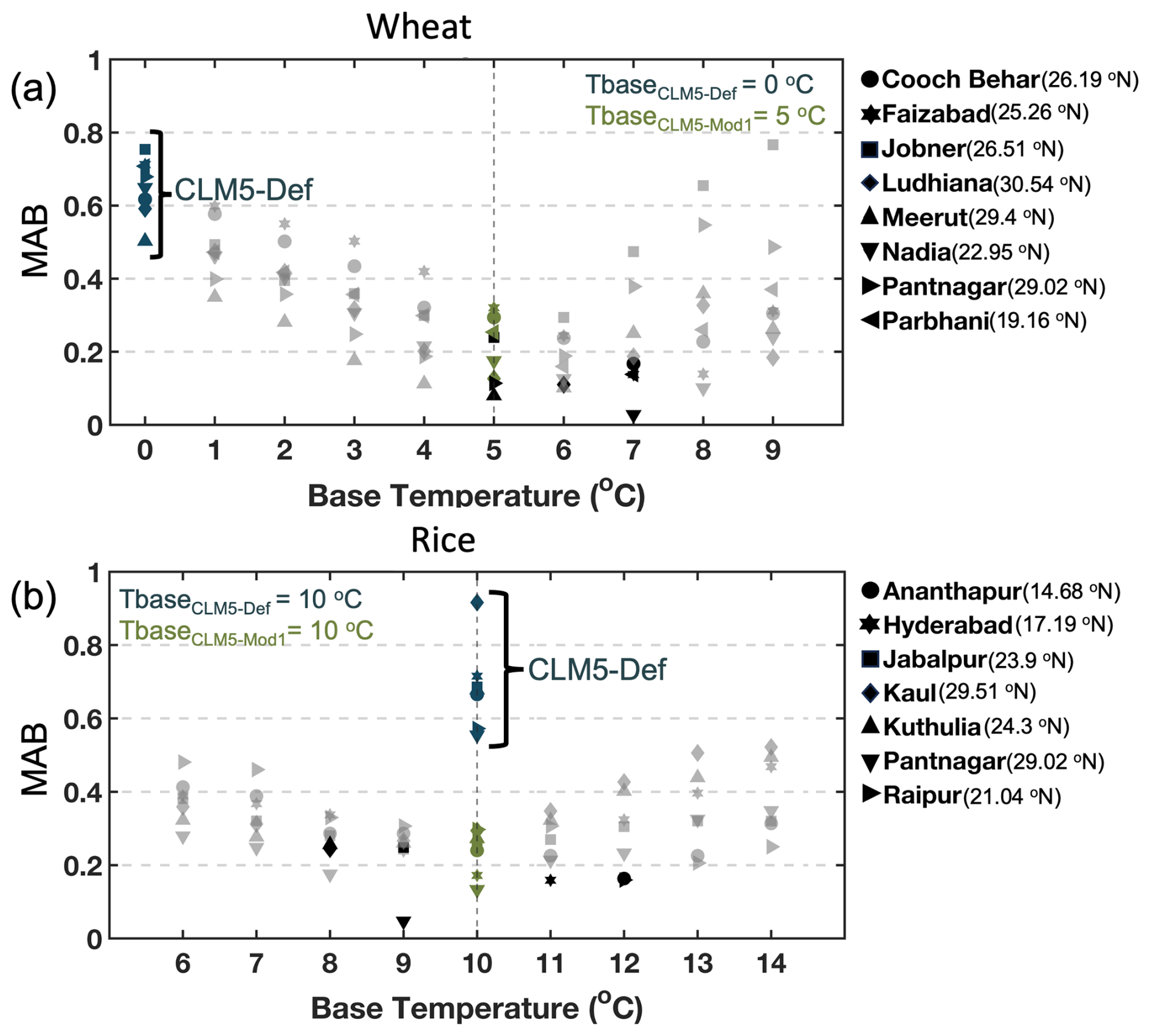
Figure 2 The overall bias in the site-scale simulations during the sensitivity study of base temperature (x axis) for (a) spring wheat and (b) rice. The y axis shows the overall bias (mean of absolute bias in LAI, yield, and growing season length). The dark green markers show the bias in the Def case at a site, the light green marker shows the bias in the Mod1 case at a site, and the black marker shows the lowest bias simulated at a site. The gray markers show the bias simulated in the sensitivity study of base temperature at a site. The legend shows the name and latitude of the sites.

In the case of rice, CLM5_Def has the highest bias, ranging from 0.5–0.95 (shown as dark green markers in Fig. 2b). The difference between the CLM5_Def and CLM5_Mod1 cases is the grain fill parameter (Table 1). Using 0.65 as the grain fill value drastically improved the rice crop simulations. The bias in CLM5_Mod1 is in the range of 0.1–0.3 (markers in light green in Fig. 2b). All the sensitivity experiments used the grain fill parameter of 0.65. The sensitivity of base temperature in rice showed that the sites in the southern rice-growing regions (lower than the Tropic of Cancer, latitude < 23.5° N) have the least bias at 11 or 12 °C. The sites in the central rice-growing regions (23.5 < latitude < 29° N) have the least bias when using base temperatures of 8 or 9 °C. Finally, the sites towards the country's northern parts (latitude > 29° N) perform best at 9 °C as the base temperature. Therefore, not all sites perform optimally at a single base temperature, and a latitudinal variation in base temperature can improve the rice crop simulations.

The base temperature at which the least bias is observed at each site and the corresponding latitude are noted for wheat and rice crops (Table S3). Using the ordinary least-squares method, the values for latvary_intercept and latvary_slope are calculated, satisfying Eq. (1) for wheat and rice (Table 2 and Fig. S3). Figure S3 shows the linear fit of the base temperature at which the lowest bias is observed (Table S3) and the latitude of the site. The linear fit has a high R² of 0.64 for wheat and 0.68 for rice.

The Mod2 version of the model used these parameters. In CLM5_Mod2, we used the baset_mapping equal to “varytropicsbylat” in the CLM namelist to turn on the latitudinal variation in base temperature in the model. To incorporate the latitudinal variation for rice crops in CLM5, an addition to the code of CropType.F90 is made at line 602 (see the Supplement).

Table 2 Latitudinal variation parameters for wheat and rice.

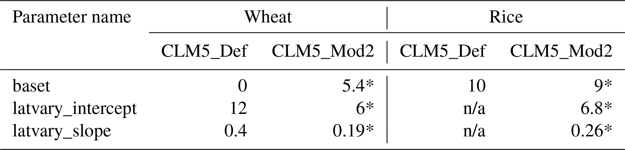
* Significant at p<0.05 using the t statistic of the two-sided hypothesis test. The notation “n/a” indicates not applicable.

2.4 Evaluation metrics

The comparison of CLM5 simulations with observations at site scale and regional scale used four evaluation parameters: mean absolute bias (MAB) (Eq. 2), root mean square error (RMSE), Pearson's r, and Kling–Gupta efficiency (KGE; Gupta et al., 2009). MAB is the normalized deviation from the observations, with values close to 0 indicating good performance. RMSE is the mean deviation of model simulations from observations. Pearson's r gives the correlation between the model estimates and observations. KGE (Eq. 3) offers a diagnostic insight into the model performance because it is a composite of correlation, bias, and variability.

$$\begin{array}{ll}\text{(3)}& {\displaystyle }& {\displaystyle }\text{KGE}=\mathrm{1}-\sqrt{(r-\mathrm{1}{)}^{\mathrm{2}}+(\mathit{\beta }-\mathrm{1}{)}^{\mathrm{2}}+(\mathit{\gamma }-\mathrm{1}{)}^{\mathrm{2}}}{\displaystyle }& {\displaystyle }\mathit{\beta }={\displaystyle \frac{{\mathit{\mu }}_{\text{CLM}}}{{\mathit{\mu }}_{\text{Obs}}}}\\ {\displaystyle }& {\displaystyle }\mathit{\gamma }={\displaystyle \frac{{\mathit{\sigma }}_{\text{CLM}}}{{\mathit{\sigma }}_{\text{Obs}}}}\end{array}$$

Here, KGE is the Kling–Gupta efficiency, r is the Pearson's coefficient between the CLM-simulated variable and observations, β is the bias ratio (ratio of means μ of the modeled and observation values), and γ is the variability ratio (ratio of standard deviations σ of modeled and observation values). KGE, r, β, and γ have their optimum at unity.

KGE is widely used in hydrological modeling because of its easy formulation and interpretation (Kling et al., 2012). KGE also makes sense from an agroecosystem point of view because we are interested in reproducing temporal dynamics, as well as preserving the spatial variation in crop growth caused by diverse climatic conditions in the Indian region, which are given by the first (β) and second (γ) moments, respectively.

A Taylor diagram (Taylor, 2001) is used to assess CLM5. The Taylor diagram summarizes the relative skill with which different models imitate the pattern in observations. The three versions of CLM5 from the study are represented by triangles on the Taylor diagram (Fig. 10). The distance between each CLM5 setup and the point displayed as a black star (observation data) on the Taylor diagram indicates how accurately each model reproduces observations. Three statistics of the simulated fields are plotted on the Taylor diagram: (a) the centered RMSE that is proportional to the distance from the point on the x axis shown as a black star (dark green contours), (b) the standard deviation that is proportional to the radial distance from the origin (gray semicircular contours), and (c) the Pearson correlation coefficient that is proportional to the azimuthal angle (light gray contours). Higher correlation, lower RMSE, and smaller standard deviation characterize the most accurate CLM5 configuration.

2.5 Model evaluation at the site scale

We compared the CLM5_Def, CLM5_Mod1, and CLM5_Mod2 simulations against the site-scale observations. We evaluated three crop variables: LAI, growing season length, and yield. We used four evaluation metrics: MAB, RMSE, Pearson's r, and KGE (described in Sect. 2.4). Because the count of observation data points is low, we used the bootstrapping method to estimate the significance of improvement from CLM5_Def to CLM5_Mod1 and CLM5_Mod1 to CLM5_Mod2. Bootstrapping is carried out with 10 000 samples for each evaluation metric, and the Student's t test is conducted to check if each model improvement performs significantly better (p<0.05) than its predecessor. Table 3 shows the abovementioned evaluation metrics. Note that 64 % of the observations are used for calibration, and the rest marked with an asterisk (*) in Table S1 are used for validation.

2.6 Model evaluation at the regional scale

2.6.1 Yield

We compared the yield simulated by CLM5 against the EarthStat yield data (Ray et al., 2012) retrieved from the “Harvested Area and Yield for 4 Crops (1995–2005)” dataset. EarthStat yield data are available at a spatial resolution of 0.1°×0.1° and are given as a 5-year average. In this study, we used the 2005 EarthStat data (representing the average yield from 2003 to 2007) regridded to 0.5°×0.5° and compared them against the CLM5-simulated yield data averaged from 2003 to 2007.

2.6.2 Irrigation

An investigation of irrigation using a climate model in Indian croplands was carried out by Biemans et al. (2016). The study highlighted the necessity of improving the cropping patterns to improve the irrigation patterns. We compared the annual mean irrigation pattern simulated by three versions of CLM5 against the annual mean irrigation water demand for wheat and rice from Biemans et al. (2016). The irrigation pattern data from Biemans et al. (2016) were unavailable as a supplement. Therefore, we extracted data from Fig. 5 of Biemans et al. (2016).

2.6.3 LAI and GPP

We compared the regional-scale model simulations against the Moderate Resolution Imaging Spectroradiometer (MODIS) 8 d GPP (MOD17A2HV006) (Running and Zhao, 2015) and LAI (MOD15A2HV0061) (Myneni et al., 2021). GPP and LAI data were retrieved from the Integrated Climate Data Centre (ICDC) website (http://icdc.cen.uni-hamburg.de/las/, last access: 4 February 2025). The MODIS GPP and LAI data mostly have four observations per month. We took the average of the observations in a month and compared them against the monthly averaged CLM5 data. We compared the MODIS monthly spatial observations with corresponding CLM5 simulations from 2001 to 2014. This exercise is to observe the spatial variation in LAI and GPP over the Indian region. We also compared the spatially averaged time series of monthly LAI and GPP over the Indian subcontinent from 2001 to 2014. This exercise is to compare the interannual cycle in MODIS observations and CLM5 simulations.

2.6.4 Latent and sensible heat flux

For the evaluation of changes in surface energy fluxes, we used FLUXCOM data (Tramontana et al., 2016; Jung et al., 2019). FLUXCOM data are generated using machine learning to merge the flux measurements in eddy covariance towers with remote sensing and meteorological data and estimate surface fluxes (Jung et al., 2019). We used the monthly 0.5° resolution RS_METEO version of the FLUXCOM data for comparison against the CLM5 simulations. We compared the monthly spatial average of heat fluxes against CLM5 simulations. We also compared the interannual time series of heat fluxes with the CLM5 simulations.

3 Results

3.1 Outcomes of model improvements at site scale

3.1.1 Wheat

LAI

The leaf area index (LAI) impacts biomass accumulation and transpiration process, while biomass distribution directly affects the yield. Furthermore, LAI is crucial in modeling multiple processes, including evapotranspiration and canopy photosynthesis. Additionally, the contact between the plant and the atmosphere is crucial in estimating the transfer of energy and matter between the canopy and the atmosphere (Su et al., 2022). Therefore, LAI is the most important of the three variables evaluated here.

Figure 3 depicts the time series of LAI simulated by the three different versions of CLM5 for different sites. Results show that CLM5_Def simulated wheat growth during April–June, while CLM_Mod1 and CLM_Mod2 simulated wheat growth in November–March. CLM5_Def simulated the wheat growth in the wrong season compared to observations. Furthermore, CLM5_Def also underestimated LAI. The seasonality error is corrected in CLM5_Mod1 to the change in the sowing window (min_and max_NH_planting_date in Table 1), but it still underestimated LAI. Including latitudinal variation in base temperature in the CLM5_Mod2 case improved the LAI simulation by reducing the underestimation at most sites except Cooch Behar (Fig. 3a and b), Faizabad (Fig. 3c–e), and a few growing seasons in Nadia (Fig. 3o). Overall, CLM5_Mod2 provided the best estimates of LAI (Fig. 4).

Figure 3 Site-scale LAI simulated by three versions of CLM5 against observations for wheat.

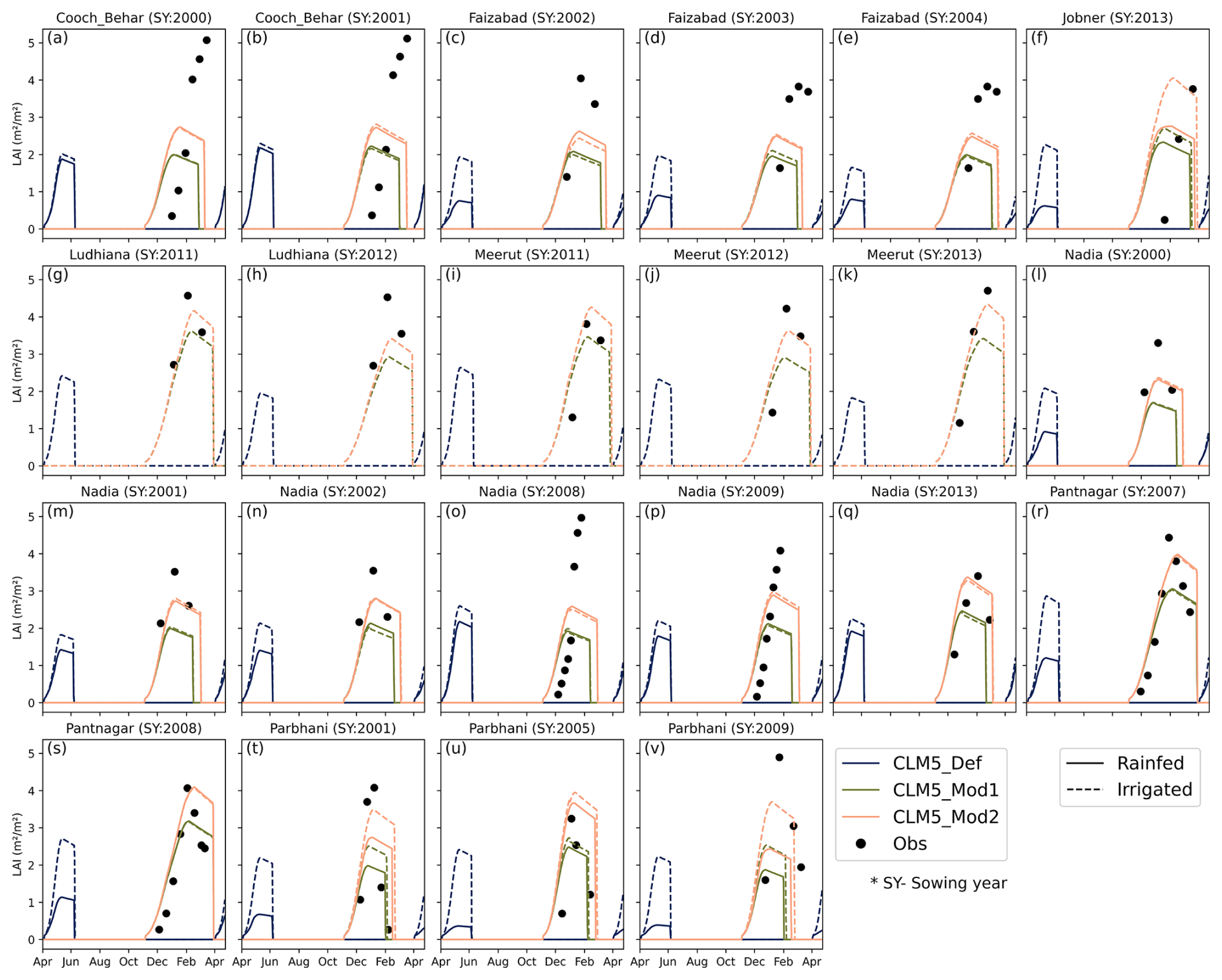
Table 3 shows the impact of improvements made to CLM5. The observed mean maximum LAI is 4.22 m² m⁻². CLM5_Mod2 is the closest to the observation with a value of 3.47 m² m⁻², while CLM5_Def is the worst with a value of 2.36 m² m⁻². Figure 3 shows us that the crop in the CLM5_Def case grows in the wrong season compared to what is observed. Hence, all performance metrics for the LAI simulations in the CLM5_Def case will show very poor results because the simulated LAI values are all zero during the observed growing season. To ensure a fairer comparison between the CLM5_Def and CLM5_Mod cases, we used days from sowing instead of calendar dates in the LAI time series. Even after adjusting for the growing season, the LAI in the CLM5_Def case has a large MAB of 0.81. CLM5_Mod1 and CLM5_Mod2 performed much better with MABs of 0.52 and 0.43. The negative r value for LAI in the case of CLM5_Def is due to the simulation of shorter growing lengths and having zero LAI values when the observations reach their maximum values. The r value improved in both the Mod cases, with a higher r value of 0.3041 (significant at p<0.01) in the CLM5_Mod2 case. KGE value is a good measure of how the model is performing in seasonality and spatially. KGE for CLM5_Def is very low (−0.62). CLM5_Mod1 showed improvement with a value of −0.02, but it is still negative. CLM5_Mod2 has the highest value of 0.19.

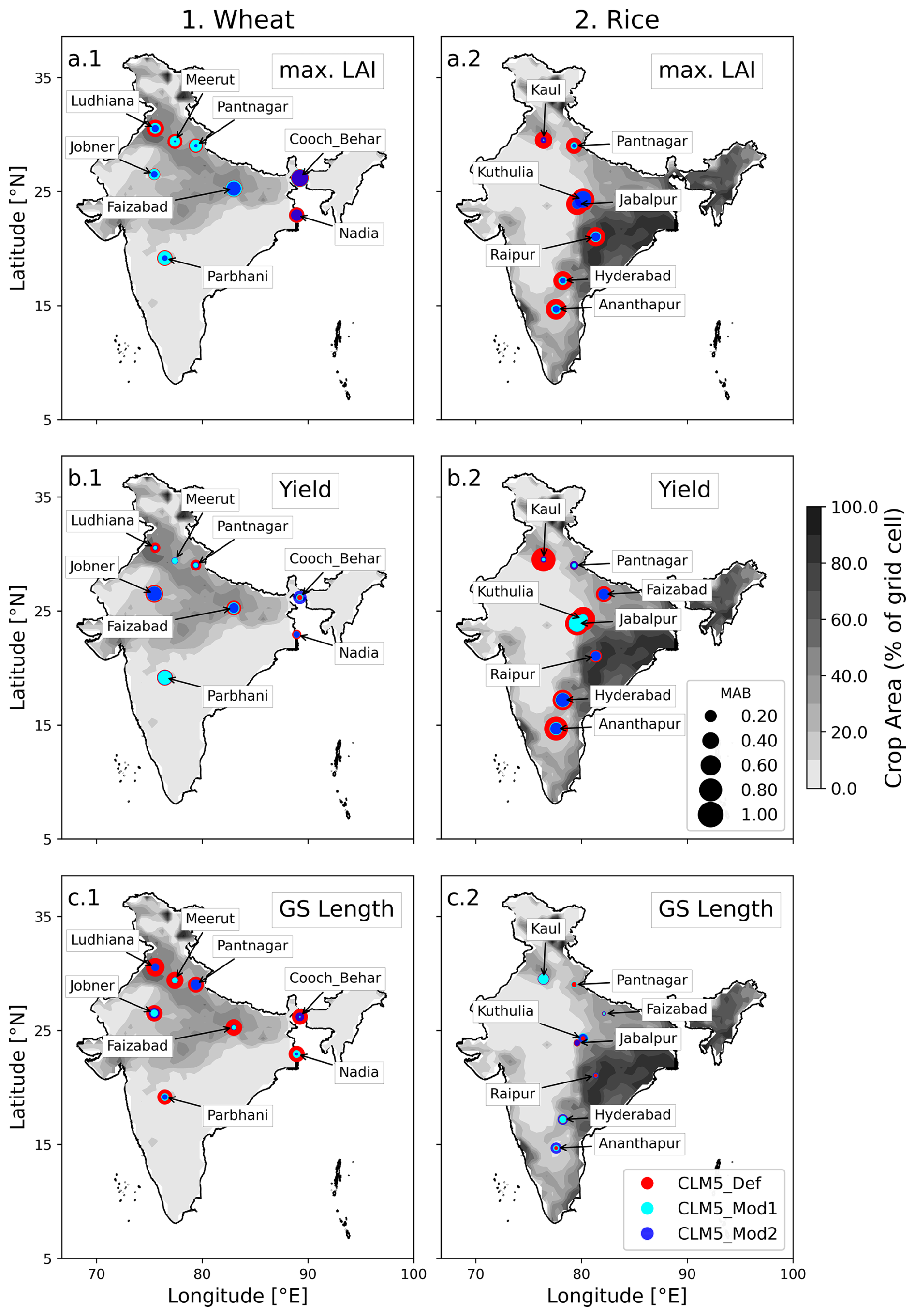
Figure 4 Site-scale CLM performance against observations for (1) wheat and (2) rice. Crop variables compared are (a) maximum LAI during the growing season, (b) yield, and (c) growing season length. The three markers at each site location show the MAB of CLM5_Def (red), CLM5_Mod1 (cyan), and CLM5_Mod2 (blue). The MAB ranges from 0 to 1. The contour on the map is the crop area per 0.5° grid cell.

Figure 4 shows the CLM5 performance in simulating crop growth at each site. The larger the marker size, the higher the bias simulated at that site. The three model versions are shown in three distinct colors, with red representing CLM5_Def, cyan representing CLM5_Mod1, and blue representing CLM5_Mod2. The improvement in LAI simulations is evident from Fig. 4a.1. The LAI simulations in Mod cases have a lower bias (smaller and the top marker) compared to the CLM5_Def case. The improvement in model simulation is not uniform across the wheat-growing region. A more significant improvement is seen in Ludhiana, Meerut, and Pantnagar, which belong to the most fertile and well-irrigated regions of India. Jobner and Parbhani also saw considerable improvement from CLM5_Def to CLM5_Mod2. These two sites belong to regions with a limited water supply. The introduction of latitudinal variation drastically improved the simulation at Ludhiana, Meerut, Pantnagar, Jobner, Nadia, and Parbhani, all belonging to distinct agro-climatic regions, proving the robustness of the model and the importance of varying base temperatures for better crop simulation.

Overall, the modified models significantly improved over the default model, with CLM5_Mod2 performing the best (Table 3 and Fig. S4).

Yield

The observed mean yield is 3.88 t ha⁻¹ (Table 3). The default model underestimated the mean yield with a value of 3.05 t ha⁻¹. The modified models performed better, simulating a mean yield of 3.68 t ha⁻¹ across all sites. All metrics in Table 3 show that the default model is the worst performer with high MAB and RMSE and low correlation and KGE values. The CLM5_Mod1 is the best performer in all metrics (bold text). It is important to note that CLM5_Mod2 performs quite well. The mean yields of CLM5_Mod1 and CLM5_Mod2 are identical, and the correlation values of 0.38 in CLM5_Mod1 and 0.30 for CLM5_Mod2 are not statistically different (significance level, p<0.05).

Site-scale comparison of wheat yield (Fig. 4b.1) highlights that the yield simulated in CLM5_Def has a high bias at all sites. The high bias in most regions is reduced by an improved growing season (CLM5_Mod1) and Tbase (CLM5_Mod2). Cooch Behar, Faizabad, and Nadia all saw improvement in wheat yield simulation from CLM5_Def to CLM5_Mod1 to CLM5_Mod2 (Figs. 4b.1 and S5). However, sites in southern (Parbhani) and northern regions (Ludhiana, Meerut, and Pantnagar) improved from CLM5_Def to CLM5_Mod1 but did not improve from CLM5_Mod1 to CLM5_Mod2 (Figs. 4b.1 and S5). The latitudinal variation in base temperature showed improvements at the sites in central wheat-growing regions, while the sites in southern and northern regions did not improve over CLM5_Mod1 (Fig. 4b.1).

Growing season length

The growing season length simulated by CLM5_Def is very short, with a mean growing season of just 69 d compared to 129 d in observations (Table 3). The growing season length considerably increased to 126 d in CLM5_Mod1 and 136 d in CLM5_Mod2. The MABs in the growing season length in CLM5_Mod1 and CLM5_Mod2 are 0.11 and 0.10, respectively, much lower than the 0.47 in the CLM5_Def case. An incorrect growing season and a lower T_base for wheat led to a very short growing-season-length simulation in CLM5_Def. The modified models performed significantly better than the default in terms of all the evaluation metrics (Table 3). Their performances are comparable, with no statistically significant difference (p<0.05) between the metrics.

Figure 4c.1 shows the MAB in the growing-season-length simulation by three CLM5 models across the sites in various climatic conditions. CLM5_Def has the largest bias, performing poorly at all sites (large red markers in Fig. 4c.1). With the improvements made in CLM5_Mod1, the growing-season-length simulation considerably improved at all sites. The changes made in CLM5_Mod2 showed mixed results. The growing-season-length simulation in CLM5_Mod2 improved over CLM5_Mod1 at Parbhani, Nadia, Pantnagar, and Ludhiana (Fig. 4c.1). Ludhiana and Pantnagar belong to very fertile regions with very low water stress. Nadia belongs to the delta region, and Parbhani belongs to an arid region. CLM5_Mod2 simulations did not show a considerable improvement over CLM5_Mod1 at Cooch Behar, Jobner, and Meerut.

The results in wheat showed that both the LAI and growing season length significantly improved in CLM5_Mod2 over CLM5_Mod1. Table S4 expands on the results discussed above to show the improvements observed during the calibration and validation stages separately. Based on the overall bias in Tables 3 and S3 and Fig. S4, we find that wheat simulation largely improved from the default to Mod2.

3.1.2 Rice

LAI

A significant improvement in LAI rice simulations can be seen in Figs. 4b.2 and  5 and Table 3, especially after introducing the latitudinal variation in base temperature. CLM5_Def underestimated the mean maximum LAI with a value of 1.65 m² m⁻², much lower than the observed 5.29 m² m⁻² (Table 3). The modified models perform much better, simulating maximum LAI in the range of 4.45–4.5 m² m⁻². We compared the CLM5-simulated LAI against the observations after correcting the difference in the growing season in CLM5_Def, as discussed in Sect. 3.1.1.1. The MAB was reduced from 0.66 in the CLM5_Def case to 0.387 in the CLM5_Mod1 case and to 0.343 in the CLM5_Mod2 case. CLM5_Mod2 LAI performed better than CLM5_Mod1 in other metrics – RMSE, r value, and KGE (Table 3) – and the improvement is significant at p<0.05.

Figure 5 Site-scale LAI simulated by three versions of CLM5 against observations for rice.

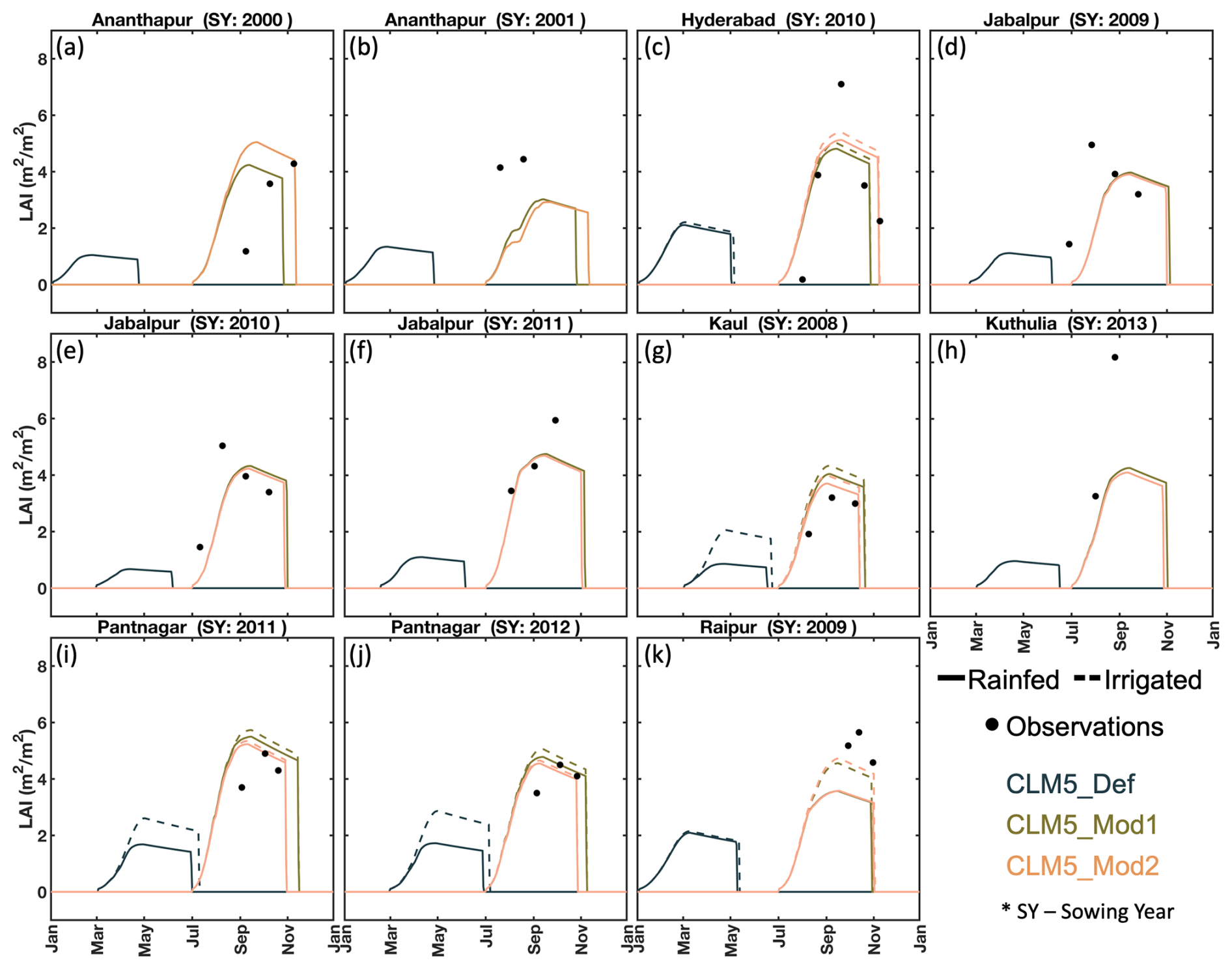
Figure 4a.2 shows the LAI simulation of rice by three versions of the model. The bias markers at each site clearly show that the changes made to the model in CLM5_Mod1 and CLM5_Mod2 significantly reduced the bias in maximum LAI simulated during a growing season. CLM5_Mod2 simulations performed better for sites in the southern (Fig. 5a–c) and northern parts of India (Fig. 5g, i, and j). The observed model improvements strongly suggest that latitudinal variation in base temperature implemented in CLM5_Mod2 is essential to capture the growth variation in LAI observed across Indian rice-growing regions (Figs. 4a.2 and S4).

Table 3 Evaluation of wheat and rice across three CLM5 setups at site scale.

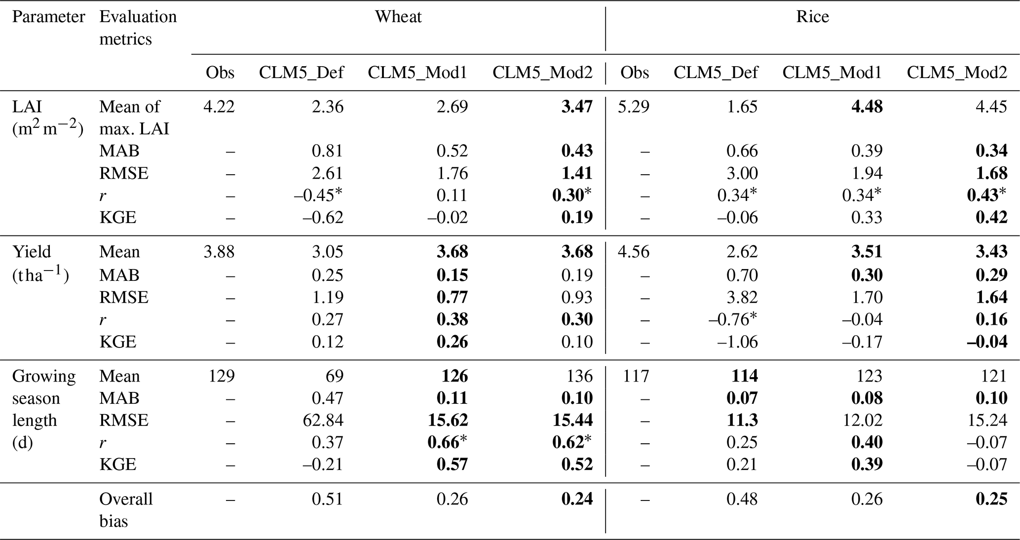
^* Significant at p<0.05 using the Student's t test. The bold font indicates the best performer in each category; if multiple models are marked in bold font, it indicates a lack of statistically significant difference between them.

Yield

The CLM5_Def yield of 2.62 t ha⁻¹ is much lower than the observed 4.56 t ha⁻¹ (Table 3). The mean yield improved by nearly 1 t ha⁻¹ in the CLM5_Mod runs but is still lower than observations. The MAB improved from 0.699 in the CLM5_Def case to 0.297 in the CLM5_Mod1 case and 0.291 in the CLM5_Mod2 case. The most significant improvement from the CLM5_Def to CLM5_Mod cases is in rice yield predictions (Table 3). RMSE improved from 1.63 t ha⁻¹ in CLM5_Def to 0.65 t ha⁻¹ in CLM5_Mod1 and 0.53 t ha⁻¹ in CLM5_Mod2. Similarly, the r value improved from –0.76 in CLM5_Def to –0.04 in CLM5_Mod1 and 0.16 in CLM5_Mod2. KGE has the best value of –0.04 in CLM5_Mod2, which is far from perfect but is much better than –1.06 in CLM5_Def and –0.17 in CLM5_Mod1. The improvement from CLM5_Mod1 to CLM5_Mod2 is significant (p<0.01), especially in terms of r value and KGE.

Figure 4b.2 highlights the significant improvement made through CLM5_Mod1 and CLM5_Mod2 in reducing the bias at all sites. The bias in CLM5_Mod1 overlaps the bias in CLM5_Mod2 at Raipur, Kuthulia, Jabalpur, Faizabad, Pantnagar, and Kaul. The biases in CLM5_Mod1 and CLM5_Mod2 are identical at all the abovementioned sites. Therefore, introducing latitudinal variation in CLM5_Mod2 has a significant impact on improving LAI simulation at all sites (Fig. 4a.2) and simulated yield better than the CLM5_Mod1, especially in the southern region (Anantapur and Hyderabad) (Figs. 4b.2 and S6).

Growing season length

The CLM5_Def model performed exceptionally well in simulating the growing season length with a value of 114 d, which is closest to the observed value of 117 d (Table 3). The MAB and the RMSE in the default case are the lowest, even though the MAB shows no significant difference among the three CLM5 versions. During our bootstrap exercise with 10 000 samples, no significant difference between MAB among the three setups was observed. RMSE in CLM5_Mod1 is lower than CLM5_Mod2. The r value in CLM5_Mod2 (–0.07) shows no variation in growing season length among the sites. However, Fig. 5 shows that the longer or shorter growing season lengths observed at the site scale are simulated in CLM5_Mod2. Figure 4c.2 shows that no version of CLM5 outperforms the others in simulating the growing season length of rice. Additionally, bias in all models is very low, less than 0.2 at most sites.

The overall bias in Table 3 and Fig. S4 for rice shows that CLM5_Mod2 performs significantly better than the other CLM5 versions. Using latitudinal variation in base temperature for rice improved the LAI and yield at all sites (Figs. 4, 5, S4, and S6). This suggests that latitudinal variation in base temperature implemented in CLM5_Mod2 is necessary to capture the growth variation observed across Indian rice-growing regions.

3.2 Outcome of model improvements at the regional scale

3.2.1 Yield

Figure 6 compares regional-scale yield simulations by CLM5 against EarthStat data (Ray et al., 2012). CLM5_Def simulations underestimated the wheat yield in central and south-central areas of the wheat-growing regions, which is also identified by Lombardozzi et al. (2020). In the CLM5_Mod1 case, the underestimation found by Lombardozzi et al. (2020) is reduced, but at the same time, an overestimation of yield is observed in the eastern parts of the wheat-growing regions. The overestimation is reduced by introducing latitudinal variation in the CLM5_Mod2 case. Large parts of the wheat-growing regions have a low bias between −1 and 1 t ha⁻¹ compared to the EarthStat data. One important region where CLM5_Mod2 is underestimating is the Punjab and Haryana regions (the northwest region in the map). In Fig. S7, we compare the total annual yield from wheat-growing regions simulated by CLM5 with FAO data. CLM5_Mod1 replicates the trend observed in FAO data. CLM5_Def underestimated the total yield owing to the shorter growing season simulated in the default case.

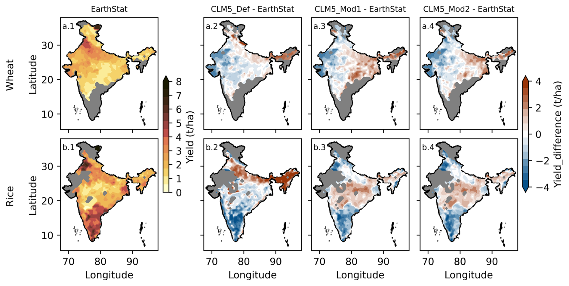
Figure 6 Yield estimates of (a) wheat and (b) rice by (column 1) EarthStat 2005 and (columns 2–4) the difference in yield between CLM5 (mean 2003–2007) versions and EarthStat data.

The CLM5_Def rice simulations underestimated the yield across large parts of the rice-growing regions and overestimated it in the Indo-Gangetic Plains (IGP) and northeast regions. CLM5 simulated a higher yield in IGP, which has a comparatively smaller rice-growing area than in the central and eastern parts of India (Fig. S8). Improved yield simulation is observed in the CLM5_Mod1 case due to changes in the growing season and grain fill threshold. The overestimation in IGP and the underestimation in southern parts of India decreased (Fig. 6b.3). However, changes made in the CLM5_Mod2 case showed slight improvement in most regions over the CLM5_Mod1 case (Fig. 6b.3 and b.4). In CLM5, rice is grown only during the kharif season; however, in the southern regions of India, where water is available throughout the year, rice is grown in two or three seasons (Wang et al., 2022). Therefore, the annual yield observations in EarthStat are higher in this region and are not reflected in the CLM5 simulations. In Fig. S7b, we compare the annual rice yield over rice-growing regions of India from CML5 simulations and FAO data. CLM5_Def overestimated the yield, considering the fact that rice grows in only one season in CLM5. With the improvements made in CLM5, the trend in FAO is matched by the modified simulations; however, yield in modified cases is lower compared to FAO data across the 15 years. The underestimation in yield is expected because rice grows in only one season in CLM5.

The improvement in rice crop growth and yield is twofold in this study: one aspect is changing the growing season, and the other is the grain fill parameter. A study by Rabin et al. (2023) used CLM5 to simulate crop yields of major crops across the globe. The important point to note here is that they used a prescribed calendar; therefore, the growing season is accurate for crops in all regions, but they did not change the grain fill parameter and used the default value of 0.4. The results for rice yield were poor compared to the FAO data (Rabin et al., 2023). Therefore, changing the growing season would not improve the yield of rice crops. Our sensitivity studies with the grain fill parameter showed that the value 0.65 produced better crop growth and yields after changing the growing season. The underestimation of yield for wheat and rice pointed out by Lombardozzi et al. (2020) is reduced to some extent with the modifications in this study. In the default case, the bias in yield, especially in rice, is around $\pm \mathrm{3}\mathrm{t}{\mathrm{ha}}^{-\mathrm{1}}$, which is reduced in CLM5_Mod2 to $\pm \mathrm{1.5}\mathrm{t}{\mathrm{ha}}^{-\mathrm{1}}$. However, more research is required to understand the reason for the bias in CLM5_Mod cases in the range of $\pm \mathrm{1.5}\mathrm{t}{\mathrm{ha}}^{-\mathrm{1}}$ in both rice and wheat.

3.2.2 Irrigation

We compared our simulated irrigation across wheat and rice-growing regions of India against the annual irrigation patterns from Biemans et al. (2016). In Fig. 7, the blue line shows the annual irrigation pattern simulated by Biemans et al. (2016), the black line depicts irrigation simulated by the CLM-Def case, and the green and orange lines show the CLM5_Mod1 and CLM5_Mod2 simulations, respectively. CLM5_Def has anomalous peaks in the pre-monsoon summer season for wheat and rice. These are also found in Mathur and AchuthaRao (2019). This error in irrigation seasonality resulted from wrong cropping patterns of wheat and rice in India in the CLM5_Def case. The modified CLM5 simulations matched the patterns from Biemans et al. (2016). One significant difference between the current study and Biemans et al. (2016) is that rice is grown in the rabi and kharif seasons in Biemans et al. (2016), while in our study, rice is sown in only the kharif season. CLM5 is not currently equipped to simulate multiple crop sowings in a year, and the rainfed and irrigated rice crop maps of CLM5 (Fig. S8) do not reflect the kharif and rabi rice crop maps. Another important point to note is that Biemans et al. (2016) reported the total irrigation water demand of the crop during the growing season, and we are comparing it with water added through irrigation to the crops.

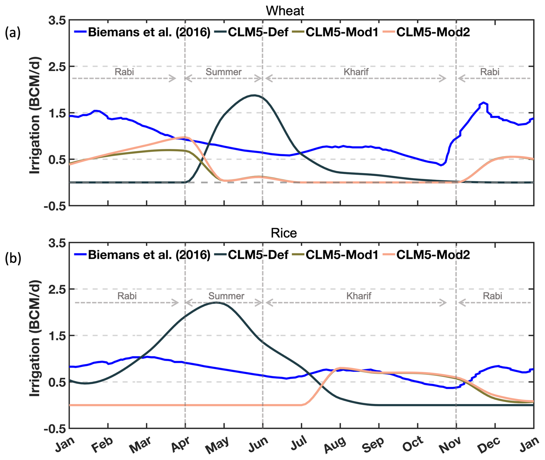
Figure 7 Comparison of water added through irrigation simulated by CLM5 and water demand data from Biemans et al. (2016).

The improvements made in our study improved the seasonality of the irrigation in wheat and rice croplands. The improved models simulate less water added through irrigation for the wheat and rice crops. Water added through irrigation over the wheat-growing region is reduced from $\mathrm{4.32}\times {\mathrm{10}}^{\mathrm{9}}{\mathrm{m}}^{\mathrm{3}}{\mathrm{d}}^{-\mathrm{1}}$ in CLM5_Def to $\mathrm{3.08}\times {\mathrm{10}}^{\mathrm{9}}{\mathrm{m}}^{\mathrm{3}}{\mathrm{d}}^{-\mathrm{1}}$ in CLM5_Mod1 and $\mathrm{3.53}\times {\mathrm{10}}^{\mathrm{9}}{\mathrm{m}}^{\mathrm{3}}{\mathrm{d}}^{-\mathrm{1}}$ in CLM5_Mod2. The drastic difference in irrigation water added is because wheat is now growing in the rabi season in the Mod cases compared to the summer season in CLM5_Def. A more significant reduction in irrigation water added to crops is observed in the case of rice. CLM5_Def simulates $\mathrm{8.09}\times {\mathrm{10}}^{\mathrm{9}}{\mathrm{m}}^{\mathrm{3}}{\mathrm{d}}^{-\mathrm{1}}$ of water added through irrigation, while CLM5_Mod1 and CLM5_Mod2 simulate only 2.97 and $\mathrm{3.09}\times {\mathrm{10}}^{\mathrm{9}}{\mathrm{m}}^{\mathrm{3}}{\mathrm{d}}^{-\mathrm{1}}$, respectively. Such drastic differences in water added through irrigation will significantly impact the hydrological cycle.

3.2.3 GPP and LAI

Spatiotemporal variation

The monthly spatial patterns of simulated GPP and LAI are shown in Figs. 8 and 9. The primary crop-growing months are June to March. This is evident in the MODIS GPP and LAI observations. However, the CLM5_Def simulated low GPP and LAI during this period. This is due to the error in the crop calendar in the default model. CLM5_Def simulated maximum carbon uptake (GPP) and LAI in April and May (Fig. 8: April and May) when very little vegetation activity is observed across India, which is also evident from MODIS GPP and LAI data (Fig. 9: April and May). In contrast, the modified models simulated the GPP and LAI cycle as observed in the MODIS data with high GPP and LAI during June–March and low values during the rest of the year.

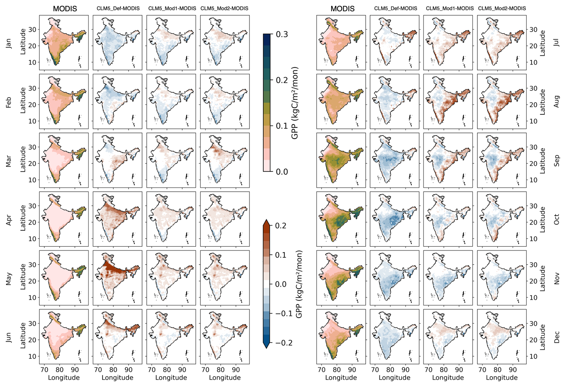
Figure 8 Spatial variation of GPP simulated by CLM5 against MODIS data. The data show the monthly GPP averaged over 2000–2014.

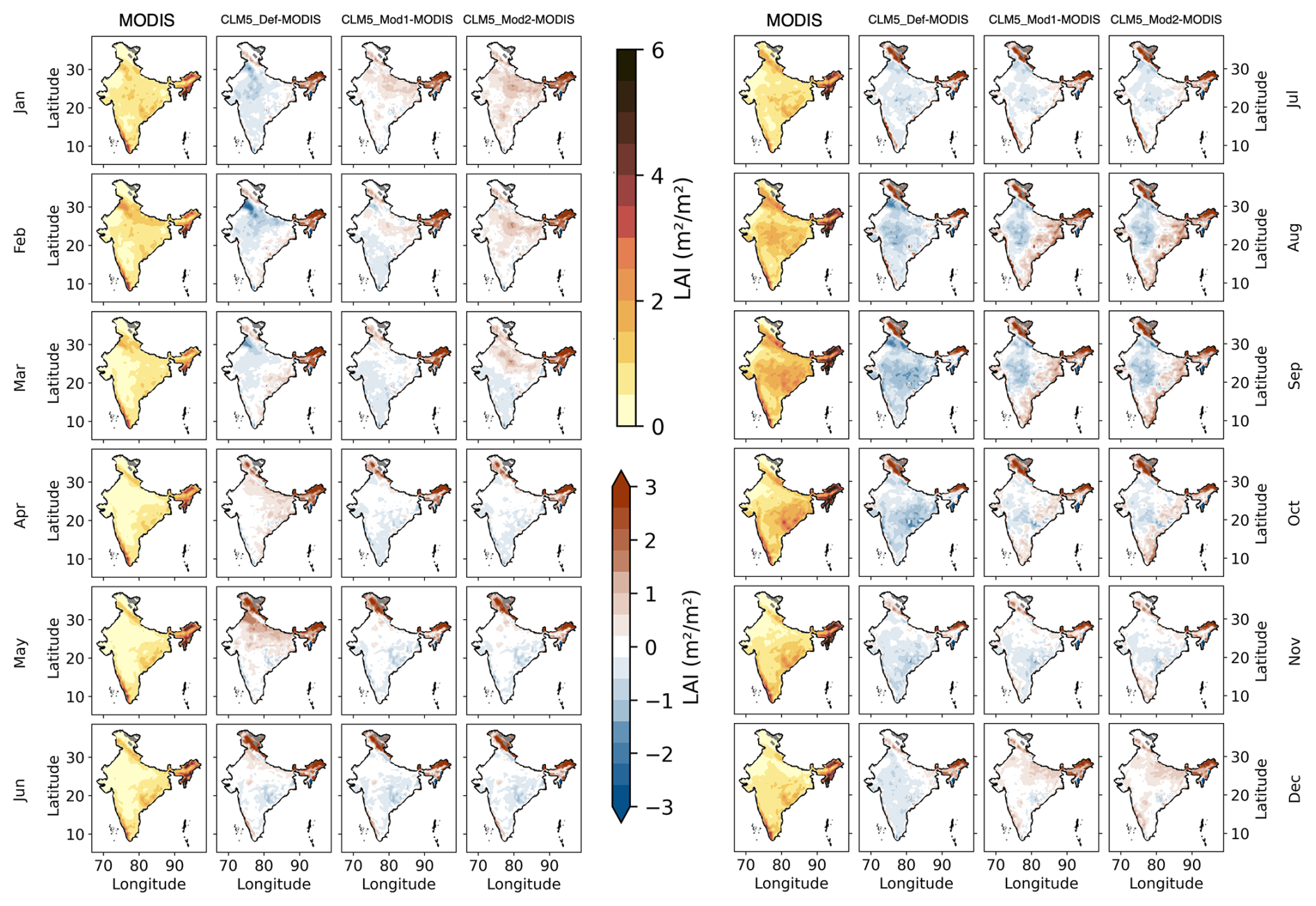
Figure 9 Spatial variation of LAI simulated by CLM5 against MODIS data. The data show the monthly LAI averaged over 2000–2014.

The maximum observed GPP in the MODIS data is in the northeast and peninsular regions of India. In contrast, the maximum GPP simulated by CLM5_Def is in the IGP region. The CLM5_Mod1 and CLM5_Mod2 simulations are similar to the MODIS observations with maximum LAI in the central and eastern parts of the country from July to February of the year. Even though the modified models captured the observed spatial patterns, they tend to overestimate the magnitudes.

Monthly time series

We evaluated the monthly time series of GPP and LAI from 2000 to 2014 (Table 4; Fig. S9). The simulated GPP performed better in the modified versions of CLM5 than the default one. The monthly mean GPP has a MAB of 0.51 in CLM5_Def, 0.241 in CLM5_Mod1, and 0.235 in CLM5_Mod2. The RMSE decreased from 6.95 kg C m⁻² per month in CLM5_Def to 3.48 kg C m⁻² per month in Mod1 and 3.56 kg C m⁻² per month in Mod2. The most significant improvement in the model simulations is seen in the correlation of CLM5-simulated GPP against the MODIS observations. The r value is negative in the case of CLM5_Def (–0.47) because the seasonality of vegetation growth in the Indian region is incorrect. The r value improved to 0.76 in CLM5_Mod1 and CLM5_Mod2. Similarly, KGE has a negative value (–0.48) in CLM5-Def and improved to 0.72 in CLM5_Mod1 and 0.71 in CLM5_Mod2.

The peaks in annual GPP from 2001 to 2014 (in Fig. S9a) in the case of CLM5_Def are off by at least 3 months compared to MODIS GPP, while the peaks in CLM5_Mod1 and CLM5_Mod2 are consistent with the observations. Figure 10b shows the monthly GPP comparison of CLM5 simulations against MODIS data in a Taylor diagram. Higher correlation, lower RMSE, and smaller standard deviation characterize the most accurate CLM5 configuration, as seen in the closer proximity of CLM5_Mod2 markers to the observational reference point. A drastic improvement is observed from default to modified cases; the correlation improved along with standard deviation, which got very close to observations (black star on the Taylor diagram) in the modified cases. CLM5_Mod2 is the best-performing setup in Fig. 10b, with high correlation and low standard deviation.

Interestingly, not all evaluation metrics for LAI improved with changes made to CLM5 in this study. The monthly mean LAI had a MAB of 0.19 in the CLM5_Def case, 0.24 in the CLM5_Mod1 case, and 0.3 in the CLM5_Mod2 case. RMSE in CLM5_Def is 0.27 m² m⁻², which increased to 0.29 m² m⁻² in the CLM5_Mod1 case and 0.35 m² m⁻² in the CLM5_Mod2 case. The overestimation of LAI is consistent across all CLM5 simulations (Fig. S9b). The overestimation of LAI by process-based vegetation models compared to MODIS LAI data is widely reported (Fang et al., 2019). The reasons are processes like carbon fixation and allocation of biomass to leaves in the models (Gibelin et al., 2006; Richardson et al., 2012), differences in defining the LAI by various models and MODIS (Fang et al., 2019), and inherent bias in LAI estimation in MODIS in the equatorial region (20° S to 15° N) (Fang et al., 2019; Lin et al., 2023). Figure S9b illustrates that although the bias is higher in Mod cases, the peaks in annual LAI in MODIS data are captured accurately by the Mod cases. The CLM5_Def peak in LAI is off by 2 to 3 months.

Table 4 Evaluation of CLM5 simulations at the regional scale against MODIS (LAI and GPP) and FLUXCOM (LH and SH) data. The bold text indicates that the version of CLM5 performed the best.

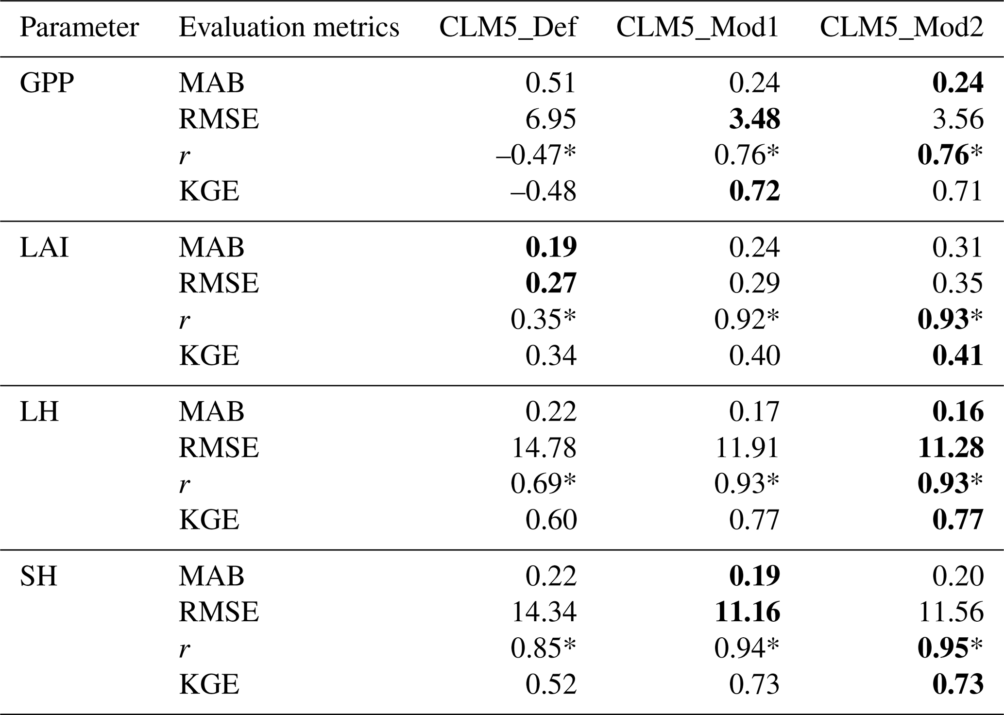
* Significant at p<0.01 using the Student's t test.

Other evaluation metrics of LAI showed that the modified models perform much better than the default case. The r value in CLM5_Def is 0.35, which increased to 0.92 in the CLM5_Mod1 case and 0.93 in the CLM5_Mod2 case. Higher r values in modified runs imply that the seasonality of LAI simulated by CLM5 considerably improved due to the improvements made in the model. The KGE metric showed improvement from 0.35 in the CLM5_Def case to 0.4 in the CLM5_Mod1 case and to 0.41 in the CLM5_Mod2 case (Table 4). The Taylor diagram of LAI (Fig. 10a) shows improvement in correlation, but the error and standard deviation are higher than the observations.

3.3 Heat fluxes

3.3.1 Latent heat flux

Spatial variation

The spatial and monthly variation in the CLM5 simulation of LH is illustrated in Fig. S10. Most of the spatial pattern in observed LH is captured by all setups of CLM5. However, one error in the case of CLM5_Def is observed in March, April, and May, where the IGP region shows high LH values absent in FLUXCOM observations. This erroneous high LH in this region is due to the wheat growth evident from Fig. 9. The least LH is observed during the winter months of November to February across all CLM5 simulations.

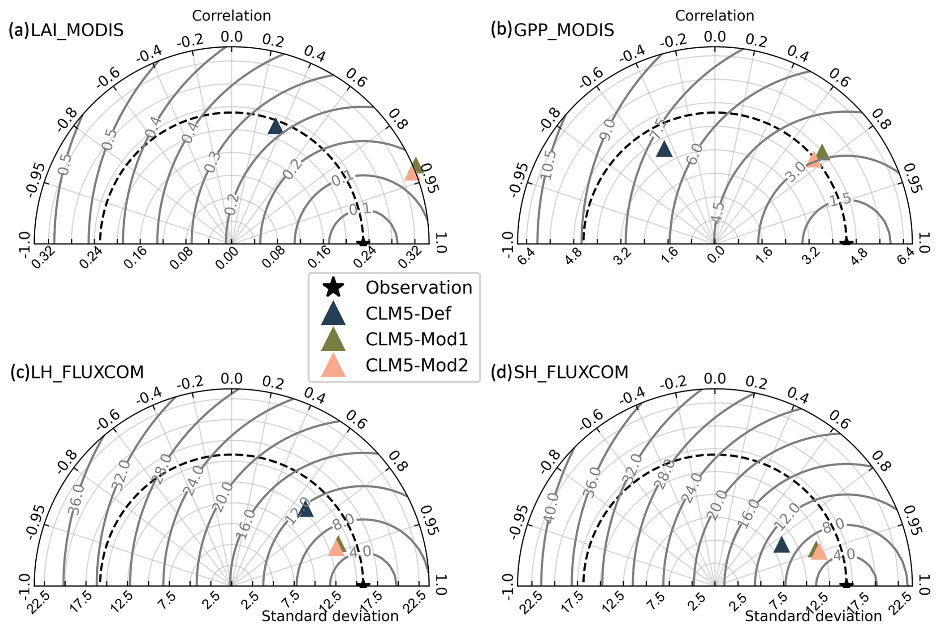
Figure 10 Comparing CLM5-simulated (a) LAI, (b) GPP, (c) LH, and (d) SH against observations. The data used here are the monthly mean from 2000 to 2014.

Monthly time series

Comparing the latent heat flux (LH) simulated by CLM5 with FLUXCOM data, we observe that the MAB of the LH was reduced from 0.22 in CLM5_Def to 0.27 in CLM5_Mod1 and 0.16 in CLM5_Mod2. The RMSE was reduced from 14.74 W m⁻² in CLM5_Def to 11.91 W m⁻² in CLM5_Mod1 and 11.28 W m⁻² in CLM5_Mod2. The correlation improved from 0.69 in CLM5_Def to 0.93 in the CLM5_Mod1 and CLM5_Mod2 cases. The KGE metric improved from 0.70 in CLM5_Def to 0.77 in CLM5_Mod cases. The improvement is evident in the Taylor diagram (Fig. 10c). CLM5_Mod simulations are much closer to the observations than the CLM5_Def case. CLM5_Mod1 and CLM5_Mod2 have similar performance, even though LAI improved in CLM5_Mod2 over CLM5_Mod1. Figure S12a shows that the CLM5 simulations underestimate the LH compared to FLUXCOM data.

3.3.2 Sensible heat flux

Spatial variation

The spatial and monthly variation in the CLM5 simulation of SH is illustrated in Fig. S11. Most of the spatial pattern in observed SH is captured by all setups of CLM5. However, CLM5_Def simulated slightly lower SH than the modified model simulations, especially from March to June. Low SH is observed from August to December across all CLM5 simulations.

Monthly time series

Comparing the sensible heat flux (SH) simulated by CLM5, we observed that the MAB of SH was reduced from 0.22 in CLM5_Def to 0.19 in CLM5_Mod1 and 0.20 in CLM5_Mod2. The RMSE was reduced from 14.34 W m⁻² in CLM5_Def to 11.16 W m⁻² in CLM5_Mod1. The RMSE in CLM5_Mod2 is 11.56 W m⁻², slightly higher than in the CLM5_Mod1 case. The correlation improved from 0.85 in CLM5_Def to 0.94 in CLM5_Mod1 and 0.95 in CLM5_Mod2. The KGE metric improved from 0.52 in CLM5_Def to 0.73 in CLM5_Mod cases. The SH in CLM5 is affected by vegetation temperature and ground temperatures. The results suggest that a difference in vegetation temperatures is observed between CLM5_Def and CLM5_Mod1, and little to no difference is observed between CLM5_Mod1 and CLM5_Mod2. The difference in vegetation temperature is likely caused by the accurate representation of the growing season in CLM5_Mod cases compared to CLM5_Def. This is also evident from the Taylor diagram (Fig. 10d), where we see improvement from CLM5_Def to CLM5_Mod1, but CLM5_Mod1 and CLM5_Mod2 markers overlap. Figure S12b shows that the CLM5 simulations underestimated the highs and lows of SH in FLUXCOM data. The peak of SH in all CLM5 simulations is in line with the FLUXCOM data. However, CLM5_Def has a larger bias in estimating the maximum SH during a year.

Overall, the improvements in the representation of the two major Indian crops drastically improved the surface energy flux simulations by CLM5 (Fig. 10b–d).

4 Discussion

In this study, we improved the representation of wheat and rice, the two major crops grown in India, in the CLM5 land model. One major strength of the current study is using multiple site-scale observations for calibrating and validating the crop modules in CLM5. Studies such as those by Gahlot et al. (2020), who looked at Indian crops, used only one site for calibrating and evaluating their model. Even studies carried out for winter wheat across the globe (Lokupitiya et al., 2009; Lu et al., 2017; Boas et al., 2021) used two or three sites for calibrating the model. In contrast, we used 33 growing seasons from 14 sites, resulting in a rigorous calibration and evaluation exercise. The improved model in our study not only simulated crop phenology better but also improved the simulation of energy and water fluxes. The results demonstrate the importance of accurate representation of crops in land surface models, especially in a country like India, where more than 50 % of land is used for agriculture.

This study looked at the variability in yield simulations at a regional scale for two major Indian crops. When compared against the EarthStat 2005 yield data, few regions showed improvement from the default CLM5 version to the modified version. Nevertheless, the yield simulated by CLM5 for wheat and rice needs improvement. Yield is now calculated as the available dry matter allocated to the grain after the allocation to the root, leaf, and stem. Global studies like Rabin et al. (2023) have highlighted the issue of inconsistent improvement in yield estimates at different scales while analyzing the interannual and spatial variation in yield estimates. A recent study by Yin et al. (2024), which looked at the yield estimates by various models, concluded that CLM5 simulated the temporal variability well but failed to simulate the spatial variability across China's wheat- and rice-growing regions. Similarly, in our study, we found an improvement in site-scale yield estimates over different growing seasons but found mixed results in regional yield estimates. The yield should perform better since CLM5 simulates the GPP with lower bias and improved seasonality. However, that is not the case here. Therefore, an investigation into the yield estimation, especially wheat in CLM5, is necessary.

A region with significant agricultural coverage and practices is misrepresented in the most widely used land surface model. Our study improved the model representation of the two major Indian crops. Our future goal is to study the feedback in the land–atmosphere system using the improved land model. The enhanced crop representation and management practices will impact the water cycle and local and global temperature and precipitation (Mathur and AchuthaRao, 2019). Rice and wheat constitute 80 % of India's harvested land area, followed by maize, sugarcane, and cotton. Improving parameterizations for all these Indian crops (seasonal and cash crops) would be an ideal next step.

While our study made progress in correcting shortcomings, it is critical to recognize that CLM5, like any sophisticated climate model, is still a work in progress. Future improvements should address broader model deficiencies highlighted in our study and various other studies. The deficiencies include the inclusion of sophisticated plant and soil hydraulics (Boas et al., 2021; Raczka et al., 2021), improvement in yield predictions, improved or new management practices like tillage (Graham et al., 2021), and post-harvest crop residual management. Furthermore, our research contributes to continuing attempts to improve CLM5 by addressing shortcomings in Indian crop representation. The enhancements are a step forward, emphasizing the iterative nature of model development and the importance of constant refinement to ensure the accuracy of the model in replicating complex Earth system processes. Future studies should build on these findings, including additional enhancements to address broader shortcomings in the model.

The major drawback of this study is that it does not consider the multiple croppings of rice followed in major parts of India. Although the harvested area of rice grown in the rabi and summer seasons is very low (Biemans et al., 2016), it is important to include the rice growth in these seasons in LSMs. This will significantly impact the terrestrial fluxes at the local scale (Oo et al., 2023). The lower LH simulated by the CLM5 models during the rabi and summer season (November to June) compared to FLUXCOM data (Fig. S12a) might be due to growing rice in the kharif season only. However, because of the small areal coverage of rabi and summer rice, their impact on large-scale fluxes and weather/climate is likely to be small. This study did not consider other major crops, such as maize, soybean, and pulses, which cover substantial harvesting areas. Future studies should focus on improving the representation of these crops in CLM5 for a comprehensive study of climate impacts on Indian agroecosystems.

5 Conclusion

Two major modifications were made to CLM5 in this study. First, the representation of wheat- and rice-growing seasons in India was improved to align better with the observations. Second, a latitudinal variation in base temperature was implemented to capture the crop varieties grown across diverse Indian agro-climatic conditions. These modifications resulted in the following improvements in the CLM5 simulations.

• The crop phenology is realistic in the modified models. The models simulate rice and wheat growth in the seasons they are grown in the field.

• The LAI simulations are significantly better in wheat and rice at the site scale – the bias in the simulations was reduced by nearly 50 % compared to the default model.

• The simulated growing season length for wheat is significantly better at the site scale. The RMSE improved from over 60 d in the default model to just over 15 d.

• The simulations of rice yield are significantly better at both site and regional scales.

• The carbon uptake (GPP) simulations over the Indian region are significantly better, improving from a negative correlation in the default model to a high positive correlation.

• The seasonality of simulated irrigation patterns across crop regimes in India is realistic.

Irrigation is a significant part of agriculture in India. With the improvements made to the model, irrigation patterns improved drastically and are now in line with a study by Biemans et al. (2016). The amount of water taken up by the crops through irrigation during their respective growing seasons decreased, and at the same time, the latent heat simulations improved from the default case.

CLM5 defines its crop parameters globally and, therefore, has a significant bias in regions such as India, where crop practices are unlike those in Europe or North America. This study demonstrated that global land models must use region-specific parameters rather than global ones for accurately simulating vegetation and land surface processes. Such improved land models will be a great asset in investigating global and regional-scale land–atmosphere interactions and developing improved future climate scenarios. Models that can simulate regional crop and land processes accurately will be able to predict the future water demand of the crops and whether enough water sources are available to meet the needs. They can also help provide estimates of the productivity and net carbon capture abilities of agroecosystems in future climate.