FZStats v1.0: a raster statistics toolbox for simultaneous management of spatial stratified heterogeneity and positional dependence in Python

Focal and zonal statistics are fundamental tools in geographic information systems (GISs) for characterizing spatial patterns, yet they have traditionally addressed spatial stratified heterogeneity (SSH) and spatial positional dependence (SPD) in isolation. To overcome this limitation, we introduce FZStats v1.0, a Python 3/QT5–based toolbox that not only integrates conventional focal and zonal statistics, but also implements a novel focal–zonal mixed statistics approach capable of jointly capturing both SSH and SPD. First, we formally develop the focal–zonal mixed statistics model to address stratified heterogeneity, spatial dependence, and their interactions within a unified framework – filling a key methodological gap left by traditional approaches that cannot accommodate their co-occurrence in real-world spatial data. Second, FZStats v1.0 provides a user-friendly graphical interface for flexible configuration of neighborhood window shapes (e.g., rectangular, circular, elliptical), sizes, and statistical operations (e.g., mean, percentiles). It also supports multiprocessing and batch operations, enabling scalable computation across diverse spatial analysis tasks. Third, we validate the effectiveness and robustness of the new method through a geothermal anomaly detection case study. Across multiple years, seasons, representative target sizes, and local window radii, the focal–zonal mixed statistics consistently outperforms both focal and zonal statistics, demonstrating its superior capability in enhancing anomaly signals under complex spatial conditions. In summary, FZStats v1.0 is not only a theoretically grounded and methodologically novel tool, but also a highly adaptable and practical solution for spatial data analysis in diverse application domains.

1 Introduction

Geographic information systems (GISs) represent a milestone in the evolution of geography by providing a new paradigm for the integrated management, analysis, and visualization of spatial data (Goodchild, 1992; Bernhardsen, 2002; Longley et al., 2015). As a vital analytical module within GIS, spatial statistics enable researchers to quantify and interpret spatial patterns and relationships on the Earth's surface with unprecedented precision (Fischer and Getis, 2010; Fotheringham and Rogerson, 1994). With continued advances in GIS technology, investigators can now more easily explore the distribution, temporal evolution, and driving mechanisms of spatial variables, and spatial statistical theories and methods play an increasingly prominent role in geographical studies. Two foundational concepts in spatial statistical analysis are spatial heterogeneity and positional dependence (Goodchild and Haining, 2004). Correspondingly, zonal statistics and focal (neighborhood) statistics offer two complementary approaches. Zonal statistics partitions raster units representing the target variable into discrete zones based on predefined schemes; computes summary metrics such as mean, maximum, minimum, and sum within each zone; and renders the results as a mosaic raster layer (Singla and Eldawy, 2018; Haag et al., 2020; Winsemius and Braaten, 2024). In contrast, focal statistics defines a neighborhood around each cell according to specified window shape and size, calculates the same set of summary metrics within that neighborhood, and assigns the resulting value to the central cell; by sliding this window across all locations, it thereby quantifies how these statistics vary with the window's movement (Mathews and Jensen, 2012; Kassawmar et al., 2019; Zhang et al., 2021).

Mainstream GIS platforms such as ArcGIS and QGIS include dedicated modules for zonal statistics and focal statistics, both of which have been widely adopted in practice. From an application standpoint, zonal statistics primarily deals with spatial stratified heterogeneity (SSH) by partitioning the study area into zones based on environmental characteristics, thereby capturing SSH (Wang et al., 2016; Wang and Xu, 2017; Gao et al., 2022). For instance, vegetation growth or potential often varies markedly among zones delineated by slope and aspect, which are key drivers of vegetation dynamics (Zhang et al., 2018, 2019; Xu et al., 2020). Conversely, focal statistics focuses on spatial positional dependence (SPD) by employing moving-window or geographically weighted techniques to detect and mitigate positional effects (Tobler, 1970; Wolter et al., 2009; Wagner et al., 2018). For example, even soils or rocks with the same texture exhibit geochemical variations that diminish with decreasing distance, reflecting underlying positional dependence; consequently, spatial interpolation of element concentrations typically assigns greater weight to nearer samples (Krige and Magri, 1982; Trangmar et al., 1986; Zuo, 2014).

In practice, SSH and SPD often co-occur, manifesting as abrupt and gradual variations respectively. At broad scales, terrestrial vegetation patterns illustrate SPD through meridional, latitudinal, and altitudinal gradients driven by land–sea distribution, solar radiation, and elevation (Qiu et al., 2013; Dong et al., 2019; Shams Eddin and Gall, 2024). Conversely, local topography, microclimate, and human activity introduce sharp boundaries in vegetation cover, generating SSH – for example, stark contrasts between shady and sunny slopes (Álvarez-Martínez et al., 2014; Zhang and Zhang, 2022) and between urban and rural landscapes (Zhang et al., 2023b). Similarly, in mineral geology, stratigraphic age differences produce SSH in resource distribution (Zhao, 2002; Zuo, 2020), while internal and external geological processes impart SPD to mineralization patterns (Cheng, 2006, 2012), as modeled by geostatistics and kriging (Krige, 1951; Goovaerts, 1997; Müller et al., 2022). Therefore, effective spatial statistical analysis must integrate both SSH and SPD.

To address these challenges, previous studies have integrated SSH and SPD, developing specialized hybrid models for specific spatial–statistical objectives. For example, Zhu et al. (2019) extended traditional spatial interpolation methods – normally focused solely on spatial dependence – by introducing environmental similarity constraints and formalized the “Third Law of Geography”, which states that geographically similar contexts yield similar target-variable values (Zhu et al., 2018, 2020). In a similar vein, Zhang et al. (2019) incorporated spatial sliding-window techniques into vegetation potential assessment, resulting in a model that simultaneously considers spatial proximity and environmental similarity (Xu et al., 2020; Zhang, 2023a). More recently, Lessani and Li (2024) developed the Similarity and Geographically Weighted Regression (SGWR) model, which combines distance-based and similarity-based weights to overcome limitations of traditional geographically weighted methods that address only spatial dependency.

Although these methods successfully integrate SSH and SPD in specific tasks such as interpolation and regression, there is still no general-purpose GIS toolbox comparable to focal and zonal statistics within standard GIS workflows. To fill this gap, this study presents FZStats v1.0 (Ren and Zhang, 2024a), which unifies traditional zonal statistics and focal statistics with the novel focal–zonal mixed statistics model. Leveraging multiprocessing and batch-processing capabilities, FZStats v1.0 improves computational efficiency and optimizes usability. Moreover, from a logical perspective, focal–zonal mixed statistics can be viewed as a generalization of the two traditional approaches. Specifically, when the moving window covers – or substantially exceeds – the entire study area (i.e., window size →∞), the method converges to zonal statistics, effectively addressing SSH. Conversely, when only a single zone is defined, it simplifies to focal statistics, capturing SPD. In the more common and complex scenarios where both SSH and SPD coexist, only the mixed approach is capable of simultaneously accounting for both characteristics. Consequently, FZStats v1.0 is positioned to function as a comprehensive analytical framework for spatial studies necessitating simultaneous evaluation of SSH and SPD parameters across diverse application domains.

2 Models

2.1 Focal statistics model

The focal statistics method addresses spatial positional dependence by computing summary statistics within a defined neighborhood around each raster cell. The implementation involves three main steps: (1) defining the neighborhood window – specifying its shape (e.g., square, circular, elliptical) and size, (2) identifying the neighboring cells – locating all raster cells within the neighborhood of the focal cell, and (3) computing statistics – applying a selected statistical function (e.g., mean, sum, minimum, maximum) to the identified neighboring cells and assigning the result to the focal cell.

2.1.1 Defining the neighborhood window

Defining the neighborhood window is a fundamental step in focal statistics. This step involves specifying two key parameters: the window's shape and size. These parameters should be determined according to the spatial characteristics of the data and the research objectives. Common shape options include circular, square, and rectangular, while the window size is typically defined by the number of cells.

To implement these neighborhood windows within a computational framework, we developed three dedicated classes, each corresponding to one of the geometric shapes: rectangular, circular, and elliptical. The class structure for each window type is presented in Listing 1.

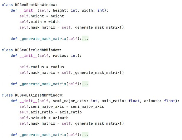
Listing 1 Code fragment for the three types of neighborhood window classes: the rectangular window class (KDGeoRectNbhWindow), the circular window class (KDGeoCircleNbhWindow), and the elliptical window class (KDGeoEllipseNbhWindow).

The mathematical essence of a neighborhood window lies in its formal specification of a spatial domain of influence. This domain is typically discretized into a two-dimensional binary mask matrix, which defines the neighborhood structure centered on a focal cell. Specifically, the mask indicates whether each cell in the local neighborhood should be considered for subsequent analysis or computation. The matrix can be formally expressed as

$$\begin{array}{}\text{(1)}& {\mathbf{NM}}_{cx,cy}(x,y)=\left\{\begin{array}{ll}\mathrm{1}& \mathrm{if}(x,y)\in {\mathrm{\Omega }}_W\\ \mathrm{0}& \mathrm{otherwise},\end{array}\right.\end{array}$$

where Ω_W denotes the neighborhood spatial domain centered on cell (cx, cy), whose geometric properties are jointly determined by the shape and size parameters of the window. As shown in Listing 1, the _generate_mask_matrix method implemented in each window class is responsible for generating the neighborhood mask matrix according to the specified window parameters (e.g., height, width, radius). For example, the implementation for a circular window is shown in Listing S1 in the Supplement.

2.1.2 Identifying cells within the neighborhood

After the mathematical formulation of the neighborhood window is established (as defined in Eq. 1), the spatial sliding window technique can be employed to identify cells within predefined neighborhoods centered on each focal cell for localized analysis (Hyndman and Fan, 1996). For a given focal cell located at position (i, j), the effective neighborhood cell set can be obtained through the following two computational stages.

1. Alignment of the neighborhood mask matrix. To ensure accurate spatial correspondence, the geometric center of the neighborhood mask matrix $\mathbf{NM}\in \mathit{\{}\mathrm{0},\mathrm{1}{\mathit{\}}}^{m\times n}$ is aligned with the focal cell located at (i, j) on the raster grid. A mapping is then established from each element in the mask matrix to its corresponding location in the raster data domain. Let the center of the mask matrix be located at (cx, cy), and let (u, v) denote the row and column offsets from the center. Then, the mapping from mask coordinates to raster coordinates is defined as

   $$\begin{array}{}\text{(2)}& (x,y)=(i+u,j+v),\end{array}$$

   where (x, y) denotes the coordinate of a neighboring cell in the raster grid, derived from the relative offset (u, v) with respect to the focal cell. This mapping ensures that the neighborhood window is precisely aligned with the focal cell.

2. Identification of the valid neighborhood cell set. To handle boundary effects when the neighborhood window extends beyond the raster extent, a boundary-clipping strategy is adopted. That is, only the cells that are entirely located within the raster data domain Ω_D are retained. The valid neighborhood cell set C_{F_valid}(i, j) is defined as

   $$\begin{array}{}\text{(3)}& \begin{array}{rl}& C_{\mathrm{F}\mathrm{\_}\mathrm{valid}}(i,j)=\\ & \left\{(x,y)\in {\mathrm{\Omega }}_{\mathrm{D}}\mathrm{|}\begin{array}{l}{\mathbf{NM}}_{cx,cy}(x,y)=\mathrm{1}\end{array}\right\},\end{array}\end{array}$$

   where ${\mathbf{NM}}_{cx,cy}(x,y)\in \mathrm{0},\mathrm{1}$ is the corresponding value in the neighborhood mask matrix. A value of 1 indicates inclusion as a valid neighbor for subsequent analysis, while a value of 0 signifies exclusion.

2.1.3 Calculating the focal statistics

After identifying the valid neighborhood cells, their corresponding values are retrieved from the raster dataset and organized into a two-dimensional array. Based on these values, statistical measures such as mean, percentiles, and other user-defined metrics can be computed. The resulting statistic is then assigned to the corresponding position in the output raster.

This procedure can be implemented through a function that obtains the neighborhood mask matrix, identifies valid neighborhood values for the focal cell, and computes the specified statistic. Listing 2 presents a representative implementation of this workflow.

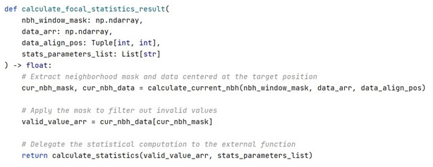
Listing 2 Python function calculate_focal_statistics_result for computing focal statistics. The function identifies valid values from a neighborhood centered at the focal cell, filters them using a predefined mask, and then calculates the specified statistics.

The computation is performed for every cell in the input raster, and the resulting values are written to the output raster, producing the final focal statistics result.

2.2 Zonal statistics model

Unlike focal statistics, which operate solely on a single value raster, zonal statistics requires two input raster layers: a value raster and a zone raster. The zone raster defines the spatial configuration and categorical labels of zones, where each cell is assigned to exactly one zone. Zonal statistics computes summary metrics (e.g., mean, sum, minimum, maximum) for each zone by summarizing the values of the corresponding cells in the value raster. The resulting statistic is then uniformly assigned to all cells within that zone. After all zones are processed, the individual results are combined to generate the final output raster.

The implementation of zonal statistics typically involves two primary steps: (1) identifying the set of cells in the value raster, corresponding to each zone based on the zone raster, and (2) calculating summary statistics across those cell values within each zone.

2.2.1 Identifying cells in the value raster falling into each zone

In zonal statistics, spatial overlay analysis is employed to associate each cell in the value raster with a specific zone, as defined by a corresponding zone raster (Hyndman and Fan, 1996). This process maps each cell in the value raster to its corresponding zone based on spatial alignment. Based on this mapping, cells in the value raster are grouped according to their zone membership resulting in a set of raster cells for each zone.

2.2.2 Calculating the zonal statistics

Once the set of raster cells belonging to each zone has been identified, a summary statistic is computed based on the corresponding cell values. The result is then uniformly assigned to all cells within that zone. After all zones are processed, the individual zone-level results are mosaicked to generate the final output raster.

Listing 3 demonstrates the implementation of this zonal statistics procedure. The calculate_zonal_statistics_result function accepts a value raster (data_arr), a zone raster (feature_arr), and a list of statistical parameters. For each unique zone code identified in the zone raster, the function identifies the corresponding cell values from the value raster, performs the specified statistical computation, and assigns the result to all cells within the zone, ultimately yielding a complete zonal statistics output raster.

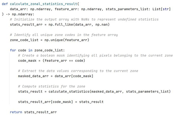
Listing 3 Python implementation of the zonal statistics computation. The calculate_zonal_statistics_result function computes a specified statistic for each zone defined in the zone raster and assigns the result to all corresponding cells in the output raster.

2.3 Focal–zonal mixed statistics

Similar to zonal statistics, focal–zonal mixed statistics operates on two raster inputs: a value raster and a zone raster. However, this method uniquely integrates both spatial and categorical criteria, combining the localized analysis of focal statistics with the zone-based constraints of zonal statistics. The computation involves two primary stages, detailed here.

2.3.1 Identifying neighborhood cells belonging to the same zone

In this step, the selection of relevant cells for analysis is governed by two criteria, the spatial proximity, as defined by a neighborhood window centered on the focal cell, and zone homogeneity, requiring that all selected cells belong to the same zone as the focal cell.

For a focal cell located at position (i, j), the valid neighborhood cell set C_{FZ_valid}(i, j) can be defined as

$$\begin{array}{}\text{(4)}& \begin{array}{rl}{C}_{\mathrm{F}Z\mathit{\_}\mathrm{valid}}(i,j)& =\left\{(x,y)\in {\mathrm{\Omega }}_{\mathrm{D}}\mathrm{|}{\mathbf{NM}}_{cx,cy}(x,y)\right.\\ & \left.=\mathrm{1}\mathrm{\Lambda }Z(x,y)=Z(i,j)\right\},\end{array}\end{array}$$

where ${\mathbf{NM}}_{cx,cy}(x,y)\in \mathrm{0},\mathrm{1}$ is the corresponding value in the neighborhood mask matrix. A value of 1 indicates inclusion as a candidate valid neighbor for subsequent analysis, whereas a value of 0 indicates that the cell is excluded. Ω_D denotes the spatial domain of the raster dataset; (x, y) denotes the relative positions of candidate neighboring cells; and Z(i, j) is the zone code of the focal cell, which serves as the categorical constraint.

2.3.2 Calculating the focal–zonal mixed statistics

Once the set of valid neighboring cells is determined based on both spatial proximity and zone membership, the next step is to compute the desired statistical measures using the identified cell values. For each focal cell, only those neighboring cells that lie within the defined spatial window and share the same zone code are included in the statistical calculation. This dual constraint ensures that the resulting focal–zonal mixed statistics reflects localized variation while maintaining consistency within categorical spatial units.

Listing 4 demonstrates the implementation of the focal–zonal mixed statistics procedure. The calculate_focal_zonal_statistics_result function computes a localized statistic for a given focal cell by integrating both spatial and zonal constraints. It first identifies the neighborhood data and associated zone codes based on the predefined window mask centered at the target position. Then, it applies a zonal constraint by retaining only those neighboring cells whose zone codes match that of the focal cell. After applying the combined focal–zonal mask, the specified statistic is computed on the resulting valid value set.

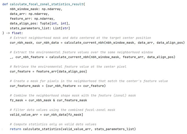
Listing 4 Python implementation of the focal–zonal mixed statistics computation. The function filters neighborhood cells based on both spatial proximity and zone code consistency and then calculates a user-specified statistic on the resulting valid subset.

The computation is performed for every cell in the input raster, where the neighborhood is constrained both spatially and categorically. The resulting values are written to the output raster, producing the final focal–zonal mixed statistics result.

3 Module design

3.1 Modeling process for focal–zonal mixed statistics

The detailed modeling process for focal–zonal mixed statistics is described as follows.

1. Preparation of the value raster and the environmental factor rasters. This initial step involves collecting and preprocessing the spatial datasets required for the analysis. The value raster typically represents the primary variable of interest, such as temperature, pollution levels, or vegetation indices. The environmental factor rasters characterize variables that potentially influence the spatial heterogeneity of the target variable, including elevation, slope, land cover, and other relevant geographical or ecological attributes. Preprocessing procedures typically include resampling, reprojection, and normalization to ensure that all raster layers share a consistent spatial extent, resolution, and coordinate reference system.

2. Construction of Unique-Value Environmental Characteristic Zonal Raster (UV-ECZR). In this step, environmental factor rasters – whether continuous or categorical – are reclassified into discrete categories using a well-defined discretization scheme. For continuous variables, the classification method should be selected according to the data distribution and research objectives: natural breaks (Jenks) are recommended for datasets exhibiting clear clustering, equal interval classification suits uniformly distributed data, and quantile classification ensures balanced representation across value ranges. For categorical variables, original classes are typically retained unless aggregating categories improves analytical validity. The optimal number of classes, usually between 5 and 8, should balance environmental heterogeneity with adequate sample size within each zone. Classification performance can be evaluated by minimizing within-zone variance, maximizing between-zone variance, and assessing clustering validity through the silhouette coefficient. After reclassification, the final UV-ECZR is produced via spatial overlay analysis, wherein each unique combination of reclassified layers is assigned a Unique-Value Environmental Characteristic Code (UV-ECC). Cells sharing the same UV-ECC form a Similar Environmental Unit (SEU), ensuring that resulting zones capture meaningful ecological thresholds while maintaining sufficient sample sizes for statistical reliability. A detailed methodological workflow for this process is provided in Sect. 3.2.1.

3. Determination of neighborhood window and statistical parameters. This process involves specifying the neighborhood window and selecting appropriate statistical parameters for the focal–zonal mixed statistics. The window size should be selected based on several considerations, including the spatial scale of the studied phenomenon (e.g., local versus regional patterns), the resolution of the input rasters (with coarser resolution favoring larger windows), and computational efficiency (as larger windows significantly increase processing time). The window shape should be chosen according to the nature of spatial anisotropy (elliptical for directional patterns), processing efficiency (rectangular shapes are computationally faster), mitigation of edge effects (circular windows help reduce boundary artifacts), and data characteristics (rectangular for grid-aligned features and circular for isotropic phenomena). The selection of the statistical function should align with the analytical objectives: the mean is suitable for general smoothing and trend detection, the standard deviation is appropriate for identifying variability and anomalies, the minimum and maximum help detect extreme values, percentiles (such as the 90th percentile) support robust threshold analyses, and the sum is useful for aggregation tasks.

4. Preparation of output raster. This step involves generating an output raster that matches the input rasters in terms of spatial extent, resolution, and coordinate reference system to ensure seamless spatial alignment. The output raster serves as a container to store the results of the focal–zonal mixed statistics computations. Before processing, the output raster is typically initialized with null values (e.g., NoData or NaN) to indicate that no computation has yet been performed. As the computation proceeds, each computed statistic is written into the output raster at the spatial location corresponding to the focal cell.

5. Calculation of the statistics. In this step, the moving window technique is employed to systematically traverse each focal cell across the study area. For each focal cell, its local neighborhood is first determined based on the predefined neighborhood window parameters (refer to Sect. 2.1.1). Within this neighborhood, cells belonging to the same SEU as the focal cell are identified by comparing their UV-ECC values. The specified statistical measure is then calculated using the corresponding values from the value raster for the selected cells. The computed statistic is assigned to the focal cell's position in the output raster. This procedure is repeated iteratively for all focal cells until the output layer is fully generated.

6. Save of output raster. After all cells have been iteratively processed, the output raster is finalized and saved to disk. Ensuring proper saving procedures, such as specifying an appropriate file format (e.g., GeoTIFF) and maintaining consistent georeferencing information, is essential to preserve data integrity and facilitate subsequent spatial analyses.

3.2 Core algorithm design for focal–zonal mixed statistics

3.2.1 Algorithm design for the UV-ECZR construction

Assume there are p continuous environmental variables, denoted as $\mathit{\{}{E}_{\mathrm{1}},E_{\mathrm{2}},\mathrm{\dots },E_p\mathit{\}}$, and their corresponding reclassified variables are $\mathit{\{}{\mathrm{CE}}_{\mathrm{1}},{\mathrm{CE}}_{\mathrm{2}},\mathrm{\dots },{\mathrm{CE}}_p\mathit{\}}$. The number of categories for CE_q is denoted as S_q, and the required digit length D_q is computed as

$$\begin{array}{}\text{(5)}& D_q=⌊{\log }_{\mathrm{10}}{S}_q⌋+\mathrm{1},\end{array}$$

where log₁₀ denotes the base-10 logarithm, ⌊.⌋ represents the floor function, and $q=\mathrm{1},\mathrm{2},\mathrm{\dots },p$. The category values for each environmental variable must be positive integers, and the value range for the reclassified raster CE_q is [1,S_q]. It is necessary to prepend a sufficient number of “0”s to ensure the code has a consistent digit length of D_q.

Thus, each pixel at location (i, j) in the raster can be represented by the vector of its p reclassified environmental category values:

$$\begin{array}{}\text{(6)}& \mathit{C}\mathit{E}(i,j)=\left({\mathrm{CE}}_{\mathrm{1}}\right(i,j),{\mathrm{CE}}_{\mathrm{2}}(i,j),\mathrm{\dots },{\mathrm{CE}}_p(i,j\left)\right),\end{array}$$

where each component CE_q(i, j) is the integer category code of the qth environmental variable at pixel (i, j).

The UV-ECC at pixel (i, j) is defined as a unique scalar encoding of the vector CE(i, j). One efficient way to construct this code is by decimal digit concatenation:

$$\begin{array}{}\text{(7)}& \text{UV-ECC}\left(i,j\right)={\sum }_{q=\mathrm{1}}^p{\mathrm{CE}}_q(i,j)\cdot {\mathrm{10}}^{{\sum }_{k=q+\mathrm{1}}^p{D}_k}.\end{array}$$

Based on the framework of raster map algebra, the UV-ECZR is constructed through a spatial overlay operation applied to the p reclassified environmental variable layers. This process corresponds to a local operation in raster algebra, where the categorical values from each layer are combined on a cell-by-cell basis to generate a multi-dimensional representation. A more realistic and pertinent code sample is provided in Listing 5.

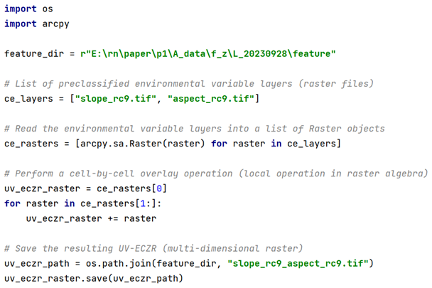
Listing 5 Python implementation of UV-ECZR generation using arcpy-based raster map algebra. Each input raster layer represents a reclassified environmental variable (e.g., slope or aspect), and the local overlay operation combines their category codes to produce a unique zone identifier for each pixel.

3.2.2 Algorithm design for determining the valid range for statistics under the sliding window technique

Rectangular windows, which align with the row and column structure of raster data, are widely used in the sliding window operations due to their simplicity and computational efficiency. However, their drawback is also evident: cells located at the four corners are significantly farther from the focal cell than those along the horizontal and vertical axes (Zhang et al., 2016a). Despite this, rectangular windows remain among the most commonly employed window shapes.

In this study, we consider not only rectangular windows but also circular and elliptical window shapes. Since a circle is a special case of an ellipse, the ellipse is used as a generalized example to illustrate the algorithm for determining the valid range of cells for statistics under the sliding window technique in the context of focal–zonal mixed statistics.

1. Mask matrix for elliptical window. An elliptical window is defined by three key parameters: the length of major axis, the ratio of the minor axis to the major axis, and the deflection angle of major axis. Let (x₀,y₀) represent the center of the ellipse, i.e., the current location; a denote the semi-major axis length; r be the minor-to-major axis ratio; and θ be the deflection angle. Then the elliptical window can be mathematically expressed as

   $$\begin{array}{}\text{(8)}& \begin{array}{rl}& \text{ellipse}(\left(x_{\mathrm{0}},y_{\mathrm{0}}\right),a,r,\mathit{\theta })=\\ & {\displaystyle \frac{[\left(x-x_{\mathrm{0}}\right)\cos \mathit{\theta }+\left(y-y_{\mathrm{0}}\right)\sin \mathit{\theta }{]}^{\mathrm{2}}}{a^{\mathrm{2}}}}\\ & +{\displaystyle \frac{[-\left(x-x_{\mathrm{0}}\right)\sin \mathit{\theta }+\left(y-y_{\mathrm{0}}\right)\cos \mathit{\theta }{]}^{\mathrm{2}}}{(ra{)}^{\mathrm{2}}}}.\end{array}\end{array}$$

   Based on Eq. (8), the bounding box of the elliptical window can be represented as ${\text{BBox}}_{\mathrm{ellipse}}(\mathrm{minX},\mathrm{maxX},\mathrm{minY},\mathrm{maxY})$, where $\mathrm{minX},\mathrm{maxX},\mathrm{minY},\mathrm{maxY}$ are as follows:

   $$\begin{array}{}\text{(9)}& \left\{\begin{array}{l}\mathrm{minX},\mathrm{maxX}=x_{\mathrm{0}}\pm \sqrt{\frac{\mathrm{4}CF}{B^{\mathrm{2}}-\mathrm{4}AC}}\\ \mathrm{minY},\mathrm{maxY}=y_{\mathrm{0}}\pm \sqrt{\frac{\mathrm{4}AF}{B^{\mathrm{2}}-\mathrm{4}AC}}\end{array}\right.,\end{array}$$

   where

   $$\begin{array}{}\text{(10)}& \left\{\begin{array}{l}A=a^{\mathrm{2}}({\sin }^{\mathrm{2}}\mathit{\theta }+r^{\mathrm{2}}{\cos }^{\mathrm{2}}\mathit{\theta })\\ B=\mathrm{2}{a}^{\mathrm{2}}\left(r^{\mathrm{2}}-\mathrm{1}\right)\sin \mathit{\theta }\cos \mathit{\theta }\\ C=a^{\mathrm{2}}({\cos }^{\mathrm{2}}\mathit{\theta }+r^{\mathrm{2}}{\sin }^{\mathrm{2}}\mathit{\theta })\\ F=-\frac{\mathrm{1}}{\mathrm{2}}\left(D{x}_{\mathrm{0}}+E{y}_{\mathrm{0}}\right)-r^{\mathrm{2}}{a}^{\mathrm{4}}\end{array}\right..\end{array}$$

   The bounding box BBox_ellipse provides a simplified and direct spatial reference for constructing a Boolean mask matrix for the elliptical window, i.e., M_{Ellipse_mask}, where cells inside and outside the BBox_ellipse are assigned values of “true” and “false”, respectively. In focal statistics, this binary mask is used directly to identify the valid neighborhood cells for statistical operations (see Fig. 1a).

2. Mask matrix for the similar environment in the bounding box. SEU is the basic object of zonal statistics. In focal–zonal mixed statistics, for the current cell, the elliptical window similar environmental unit (EW-SEU) is established according to the environmental characteristic codes within the initial neighborhood window defined by the bounding box. Using M_{Similarity_mask} to represent this unit, cells with the same environmental characteristic code as the current cell are assigned a value of “true”, while others are assigned a value of “false”, as shown in Fig. 1b.

3. Mask matrix for the similar environment in the elliptical window.

   The matrices of steps (1) and (2) share the same dimensions, and thus the similar environment mask matrix for the current cell in the elliptical window can be constructed using a logical “AND” operation between these two matrices, as expressed in the following equation:

   $$\begin{array}{}\text{(11)}& \begin{array}{rl}{\mathbf{M}}_{\mathrm{E}\mathrm{\_}\mathrm{S}\mathrm{\_}\mathrm{mask}}& ={\mathbf{M}}_{\mathrm{Similarity}\mathrm{\_}\mathrm{mask}}\\ & \wedge {\mathbf{M}}_{\mathrm{Ellipse}\mathrm{\_}\mathrm{mask}},\end{array}\end{array}$$

   where ∧ denotes the logical “AND” operator. M_{E_S_mask} serves as the basis for determining the valid range for focal–zonal mixed statistics, as illustrated in Fig. 1c.

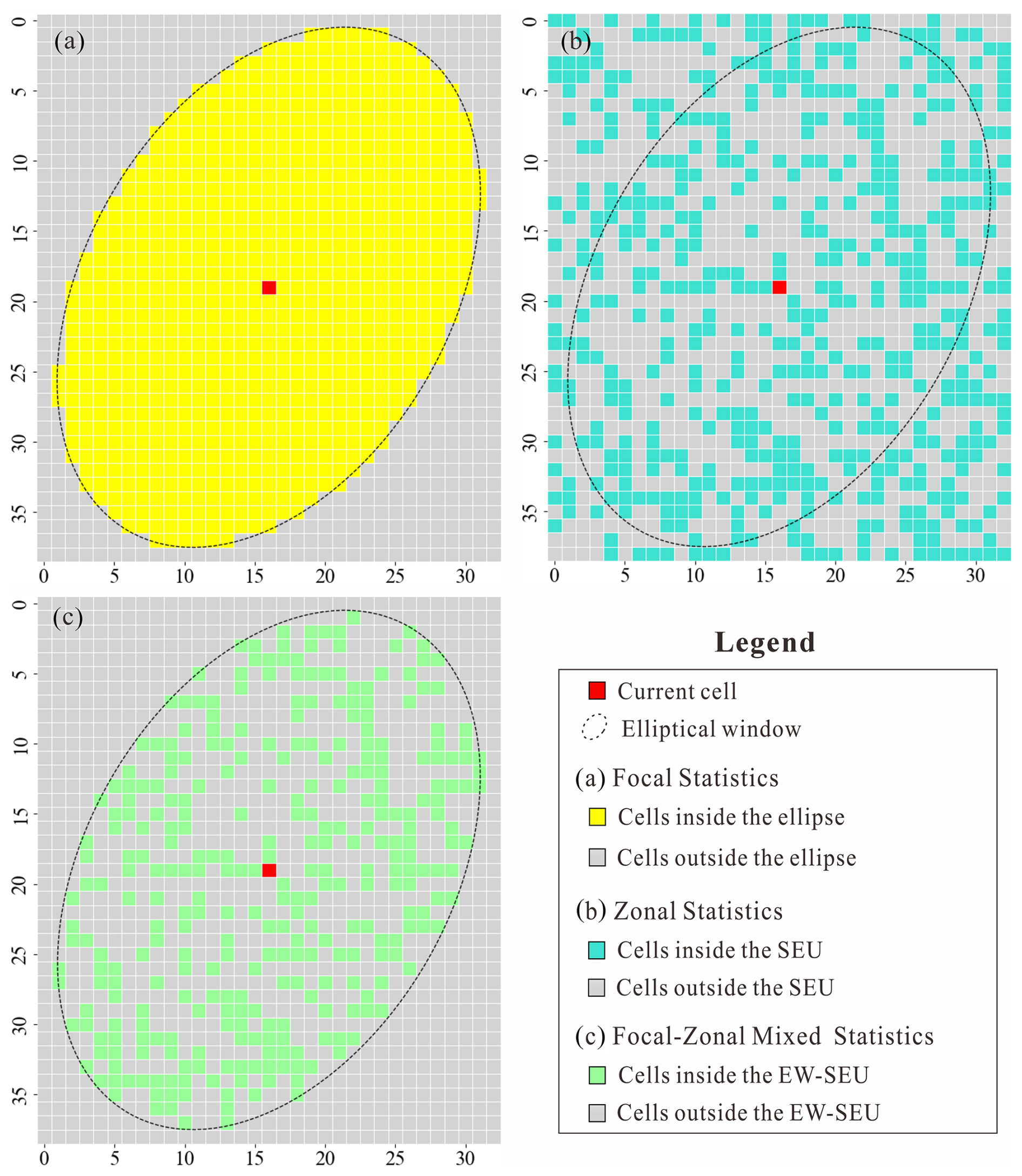
Figure 1 Heatmaps for the Boolean mask matrix: (a) the elliptical window of focal statistics, (b) the similar environmental unit (SEU) of zonal statistics, and (c) the elliptical window similar environmental unit (EW-SEU) of focal–zonal mixed statistics.

3.2.3 Algorithm design for the statistics calculation

The core algorithm for statistical computation within the focal–zonal mixed statistics framework consists of the following steps:

1. Determination of valid statistical cells in the value raster. Using M_Value to represent the cell array from the value raster within the bounding box defined above, then by performing a bitwise multiplication of M_{E_S_mask} with M_Value, the final valid statistical value matrix M_Valid is obtained:

   $$\begin{array}{}\text{(12)}& {\mathbf{M}}_{\mathrm{Valid}}={\mathbf{M}}_{\mathrm{E}\mathrm{\_}\mathrm{S}\mathrm{\_}\mathrm{mask}}\otimes {\mathbf{M}}_{\mathrm{Value}},\end{array}$$

   where ⊗ denotes bitwise multiplication. This operation collects cells from the value raster that are located within the neighborhood and share the same UV-ECC as the current cell, while masking out other cells that could interfere with the statistical results. In M_Valid, the masked cells can be represented with “NaN”.

2. Design of the calculation function for the statistics. Taking M_Valid as the final input, the calculation functions for focal–zonal mixed statistics can be designed based on scientific computing tools such as NumPy. This library provides a range of statistical methods, including minimum, maximum, mean, standard deviation, percentiles, and more. For instance, the numpy.nanmax() function automatically ignores missing values (“NaN”s) when computing the maximum of M_Valid. Similarly, the numpy.nanpercentile() function calculates the nth percentile of M_Valid while excluding “NaN”s.

3.3 User interface design

The focal–zonal mixed statistics, along with traditional zonal statistics and focal statistics, are included in the newly developed toolbox, FZStats v1.0, using Python3 and QT5. The user interface is organized into three tabs, each dedicated to one of the three methods, allowing users to switch among them (see Fig. 2). Taking the tab for focal–zonal mixed statistics as an example, the interface is divided into four main sections, and the detailed description of the user interface design is given as follows.

Figure 2 User interface design of FZStats v1.0 (Ren and Zhang, 2024a).

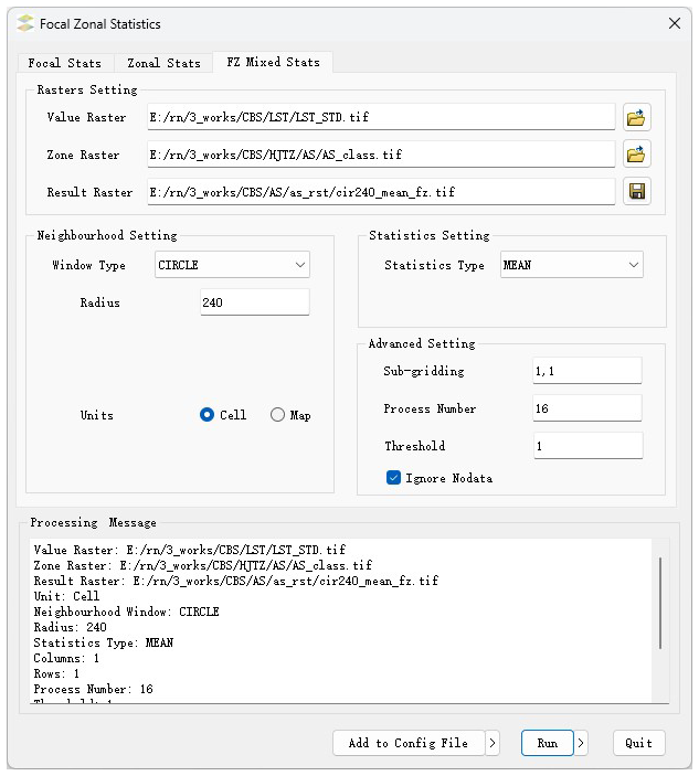
1. Input and output design. Users can load the value raster and UV-ECZR layers as inputs. Additionally, the output path and filename for the result raster can be specified.

2. Neighborhood window design. Users can define the shape (e.g., rectangular, circular, elliptical) and size of the neighborhood window. For rectangular and circular windows, size is controlled by the half-side length and radius, respectively. Elliptical windows are configured via three parameters: the length of the major axis, the ratio of the minor axis to the major axis, and the deflection angle of major axis.

3. Statistical measure design. A dropdown menu allows users to choose from various statistical measures (mean, max, standard deviation, etc.). For percentile-based statistics, the desired percentile value (e.g., 50th, 75th, 98th) must be specified.

4. Optimization settings. This section presents optimized parameter configurations to enhance computational efficiency:

   • -

     Chunk processing. Divide large raster layers into smaller chunks to manage memory usage efficiently.

   • -

     Parallel processing. Specify the number of processors to enable parallel computation and reduce runtime on multi-core systems.

   • -

     Threshold setting. Define a minimum sample threshold for statistical operations to ensure robust and meaningful results.

Additionally, a batch processing mode is provided for automation. Users can prepare a configuration file (config.ini) to set parameters for multiple runs. This facilitates efficient task management, parameter reuse, and error tracking.

4 Experimental study

4.1 Background of the case

Geothermal resources, similar to coal, oil, and natural gas, are valuable energy mineral resources, whose development and utilization play a crucial role in alleviating energy supply pressures and improving the global environment (Huang and Liu, 2010; Goldstein et al., 2011). The primary indicator for geothermal exploration is the detection of thermal anomalies (Romaguera et al., 2018; Gemitzi et al., 2021). In recent years, with the rapid advancement of remote sensing technologies, land surface temperature (LST) derived from thermal infrared bands has become a key parameter for identifying geothermal anomalies. However, LST is influenced not only by geothermal activity but also by environmental factors such as slope, aspect, and surface vegetation cover (Tran et al., 2017; Duveiller et al., 2018; Zhao and Duan, 2020).

To effectively extract LST anomalies directly related to geothermal activity, it is essential to suppress the confounding effects of surface environmental variables. Within the analytical framework of the focal–zonal mixed statistics developed in this study, terrain features are incorporated into environmental zoning, and the spatial sliding window technique is employed to mitigate environmental interference and enhance the detection of geothermal anomaly signals.

4.2 Data preprocessing

4.2.1 Spatial distribution of LST

In this study, Landsat 8 imagery (Orbit Number: 116031; https://earthexplorer.usgs.gov, last access: 3 August 2024) acquired during the spring, summer, and autumn seasons of 2015, 2019, and 2023, covering the Changbai Mountain region, was utilized for land surface temperature (LST) mapping and geothermal anomaly detection. The selection of multi-temporal images across different seasons and years was intended to robustly validate the effectiveness of the proposed method and to explore the temporal evolution patterns of geothermal anomalies, thereby providing improved support for geothermal exploration.

Following standard preprocessing procedures, including radiometric calibration and atmospheric correction, the Universal Single-Channel Algorithm (Jimenez-Munoz et al., 2009, 2014; Zhang et al., 2016b) was applied to retrieve LST across the study area. The resulting LST distributions are illustrated in Fig. 3.

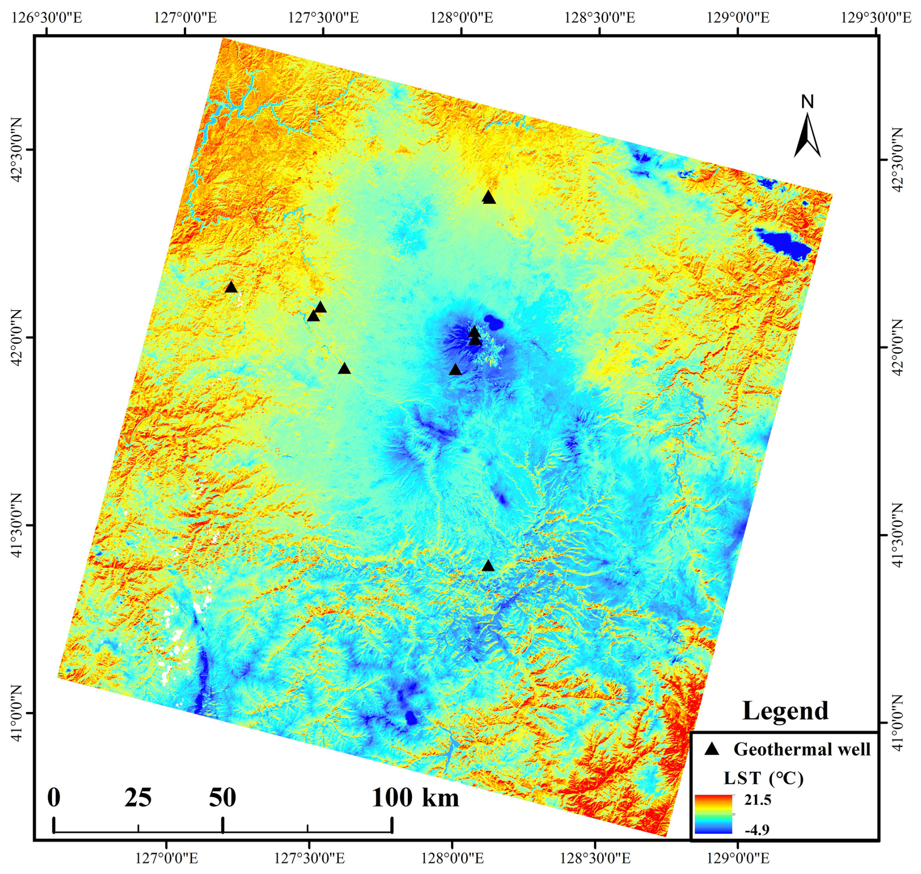
Figure 3 Spatial distribution of land surface temperature (LST) in the study area on 20 March 2023.

Taking the LST retrieved from the Landsat 8 image acquired on 20 March 2023, as an example, a comparison between Fig. 3 and the terrain information presented in Fig. 4 reveals a strong spatial correlation between LST patterns and topographic factors, particularly slope aspect. Given that the local overpass time of Landsat 8 over the study area was approximately 11:00 a.m. local solar time (10:11 a.m. China standard time, UTC+8), with a corresponding solar azimuth angle of 153°, LST values were significantly higher on southeast-facing slopes compared to northwest-facing slopes (Fig. 4a). This highlights the pronounced influence of solar radiation on the spatial variability of LST within the study area.

4.2.2 Mapping of unique-value environmental characteristic zones

Slope and aspect, derived from the original elevation data obtained via https://earthexplorer.usgs.gov (last access: 3 August 2024), were selected as the environmental factors for constructing the UV-ECZR (see Fig. 4a and b). As previously discussed, these two variables exhibit a strong spatial coupling relationship with LST. Although elevation and vegetation coverage were not directly included in the environmental zoning process, their variability can be considered relatively homogeneous within the defined neighborhood window (Zhang et al., 2019). Thus, their confounding effects are indirectly mitigated. In the framework of focal–zonal mixed statistics modeling, sample heterogeneity arising from long-range spatial variables can be effectively controlled by spatial proximity, while heterogeneity caused by short-range spatial variables is suppressed through environmental similarity.

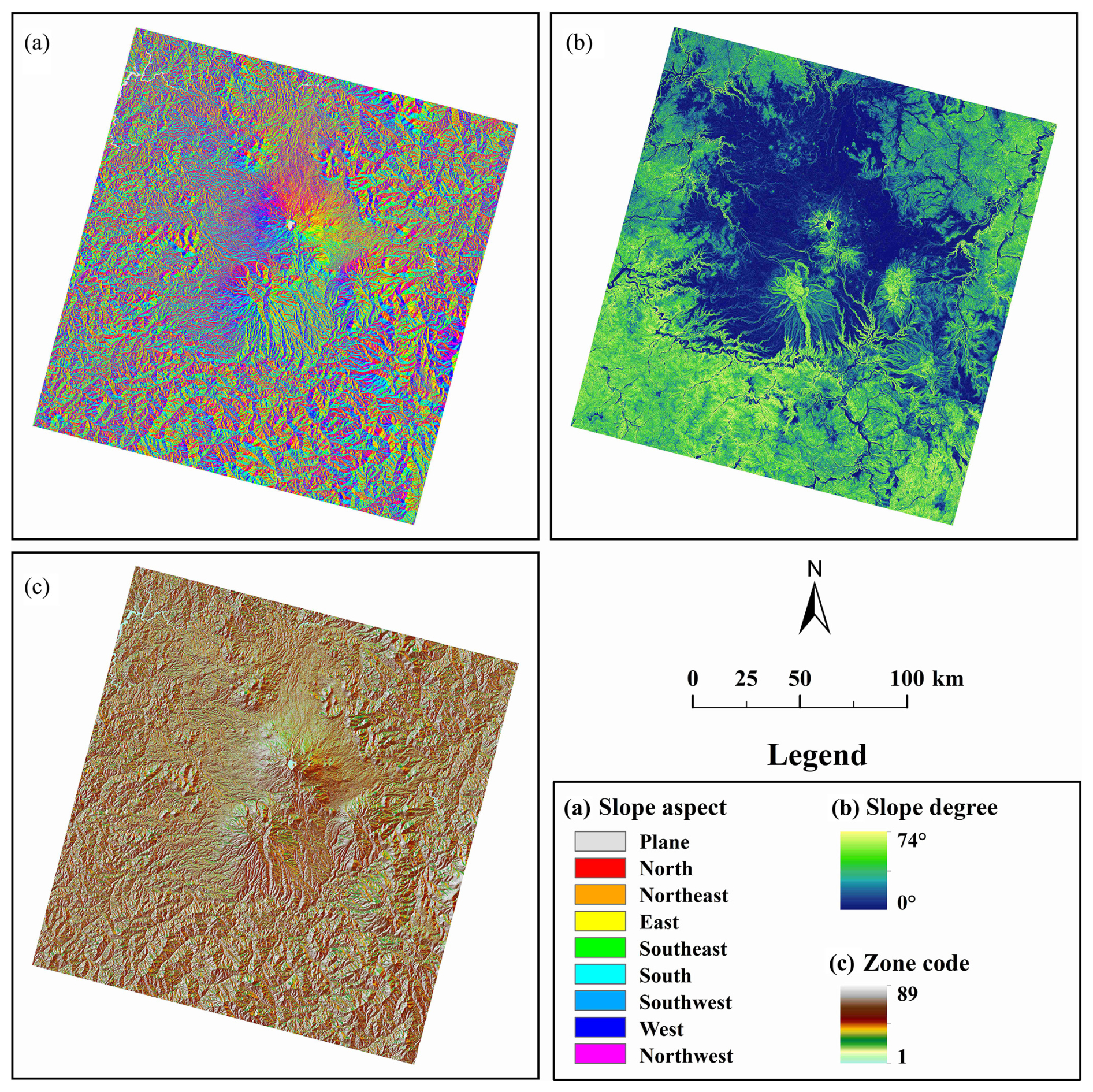
Figure 4 Maps of environmental factors: (a) slope aspect, (b) slope degree, and (c) the composite Unique-Value Environmental Characteristic Zonal Raster (UV-ECZR).

4.3 Enhancement of geothermal anomalies based on focal–zonal mixed statistics

In mineral prospectivity mapping, standard deviation normalization (Z-score transformation) is commonly employed to assist in constructing indicator variables for anomaly detection (Journel and Huijbregts, 1978; Goovaerts, 1997). This procedure involves subtracting the mean from the original value, dividing it by the standard deviation, and rescaling variables to a uniform range to mitigate scale-dependent biases and enhance comparability of multi-source geochemical data in predictive modeling (Carranza, 2008). The resulting standardized value quantifies the deviation of the original measurement from the mean in units of standard deviations. The core principle lies in defining an appropriate sample range for calculating local background statistics (e.g., mean and standard deviation), which ensures meaningful comparisons between the current value and its spatial context (Cheng, 2007; Wang et al., 2011).

In this study, focal–zonal mixed statistics was adopted to define the comparable sample range by simultaneously considering spatial proximity and environmental similarity. The source data are provided in Ren and Zhang (2024b). Specifically, for each current location, the level of land surface temperature (LST) was assessed within a sample set determined jointly by the local moving window and similar terrain features. This method effectively suppresses the influence of terrain, vegetation, and other confounding factors, allowing the resulting LST anomaly distribution to predominantly reflect geothermal activity. Using a circular moving window with a radius of 4.2 km, the enhanced geothermal anomaly map derived from Fig. 3 is shown in Fig. 5.

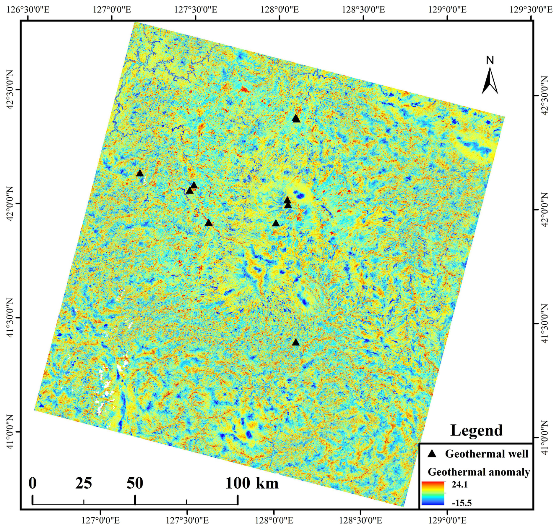
Figure 5 Enhanced geothermal anomaly map based on focal–zonal mixed statistics with a local window radius of 4.2 km.

By comparing Figs. 5 and 3, it is evident that the LST anomalies enhanced through focal–zonal mixed statistics show a stronger spatial correlation with known geothermal wells (as referenced by Yan et al., 2017). The higher values in Fig. 5 more effectively highlight these geothermal wells, suggesting that areas with high values in this figure have an increased likelihood of indicating new geothermal resources.

4.4 Performance comparison

Following the standard deviation normalization approach described above, zonal statistics and focal statistics were also applied to the LST dataset (Fig. 3) to enhance geothermal anomalies, thereby facilitating comparative evaluation of the models. Specifically, the receiver operating characteristic (ROC) curve was employed to assess the predictive performance of the original LST and the three enhancement indices derived from focal statistics, zonal statistics, and focal–zonal mixed statistics.

The ROC curve plots the false positive rate (FPR) against the true positive rate (TPR) (Fawcett, 2006; Hanczar et al., 2010), and the area under the curve (AUC) is used as a quantitative metric for model evaluation. AUC values range from 0.5 to 1, where higher values indicate better predictive accuracy and model performance.

The ROC curves for the LST dataset and the three enhancement indices are presented in Fig. 6, where subfigures a–d correspond to the four observation dates: 20 March, 24 June, 28 September, and 25 December 2023. Focal statistics and focal–zonal mixed statistics were both implemented using a circular window with a radius of 4.2 km. It is evident that, across all seasons, the enhancement indices derived from the focal–zonal mixed statistics approach consistently outperform the others. For instance, in Fig. 6a, the AUC value under focal–zonal mixed statistics reaches 0.734, notably higher than that of zonal statistics (0.508), focal statistics (0.669), and the original LST (0.474). Although both zonal statistics and focal statistics demonstrate slight improvements over the raw LST, their enhancement effects remain limited. Furthermore, comparison of Fig. 6a–d indicates that our enhanced model performs best in autumn, as evidenced by the highest AUC value observed in this season.

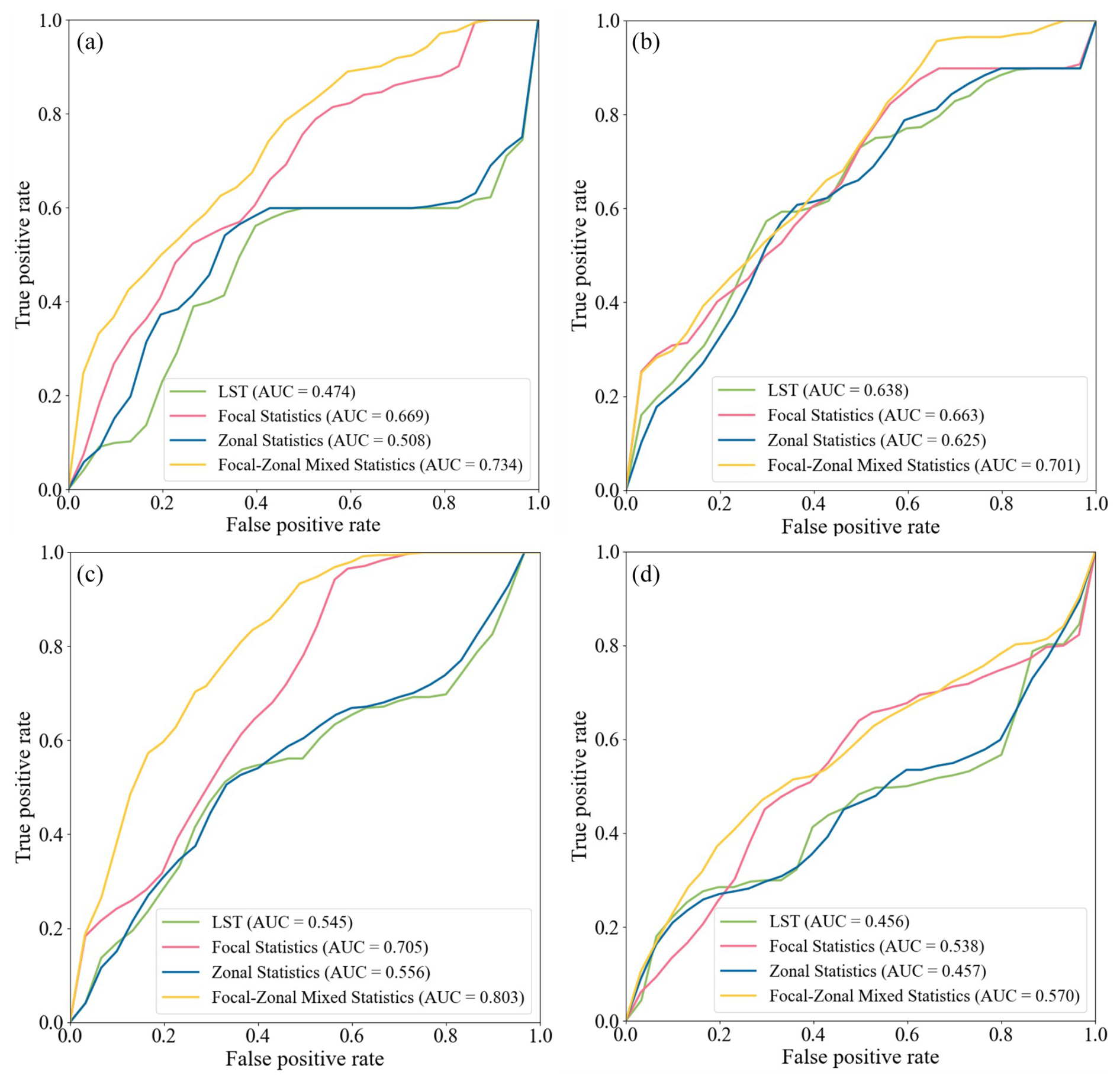
Figure 6 Receiver operating characteristic (ROC) curves of the land surface temperature (LST) and its three enhancement indicators derived from focal statistics, zonal statistics, and focal–zonal mixed statistics, respectively. Parameter settings: the local window used for both focal statistics and focal–zonal mixed statistics is a circle with a radius of 4.2 km, the zoning categories used for zonal statistics are identical to those employed in focal–zonal mixed statistics, and a geothermal well represents an area of 0.035 km² surrounding it.

5 Discussion

5.1 Significance and necessity of the new statistical method

Firstly, from a theoretical standpoint, traditional methods each address only one aspect of spatial variation: focal statistics primarily captures SPD, while zonal statistics is designed to account for SSH. However, real-world spatial problems often exhibit both characteristics simultaneously. This underscores the theoretical necessity and practical relevance of developing the new method – focal–zonal mixed statistics – which bridges the methodological gap between focal statistics and zonal statistics.

Secondly, from a conceptual perspective, focal–zonal mixed statistics can be viewed as a generalization of the two conventional approaches. When the moving window encompasses – or far exceeds – the entire study area (i.e., the window size approaches infinity), the method converges to zonal statistics, effectively capturing stratified heterogeneity. Conversely, when the analysis is confined to a single environmental zone, the method reduces to focal statistics, thereby focusing on spatial positional dependence. This flexibility enables the new method to seamlessly adapt to different spatial structures.

Thirdly, in terms of practical performance (see Fig. 6), although traditional methods show some ability to enhance geothermal anomaly detection – for example, focal statistics improves AUC values by 3.9 % to 41.1 % over the original LST – the proposed method demonstrates significantly greater efficacy, with AUC improvements ranging from 9.9 % to as high as 54.9 %. These results clearly highlight the superior performance of focal–zonal mixed statistics.

Finally, regarding broader applicability, although geothermal anomaly enhancement serves as the illustrative case in this study, the utility of the proposed method extends well beyond this specific context. It is particularly well suited for applications requiring both improved sample purity and simultaneous control over SSH and SPD. Potential domains include mineral resource potential evaluation, vegetation restoration potential assessment, cropland productivity analysis, and terrestrial vegetation carbon sink estimation. Furthermore, the method can be employed to assess the spatial variability of target variables under specific environmental constraints and to evaluate the effectiveness of environmental factors in delineating spatial patterns of interest.

5.2 Robustness of the new method

To ensure that the superior performance of the proposed method, as demonstrated in Sect. 4.4, is not due to chance, it is essential to test its robustness under varying conditions. This involves adjusting key parameters such as the size of the local analysis window, the year and season of image acquisition, and the representative area assigned to geothermal wells. Through multi-scenario comparative experiments, the consistency and reliability of the model's advantages can be systematically evaluated.

To rigorously assess the robustness of the proposed method, we conducted a series of controlled experiments involving multiple scenarios. Specifically, Landsat imagery from the years 2015, 2019, and 2023 was selected, covering all four seasons – spring, summer, autumn, and winter – for each year. Due to cloud contamination and other data quality issues, some missing seasonal scenes were replaced with imagery from adjacent years and similar months. In addition, two representative areas were defined for individual geothermal wells: 0.0009 km² (equivalent to a single 30 m × 30 m pixel) and 0.035 km² . To further test the model's sensitivity to spatial scale, we varied the radius of circular local windows from 0.3 to 9 km in 0.3 km increments. These selections of years, seasons, neighborhood sizes, and point representativeness were all deliberately designed to evaluate the stability and generalizability of the proposed method relative to the two traditional approaches.

When the representative area for a geothermal well is defined as a circle with an area of 0.035 km², and imagery from the year 2023 is used for modeling, the AUC values of the original LST and its enhancement indices are calculated across different seasons and a range of local window sizes. Specifically, circular windows with radii ranging from 0.3 to 9 km (at 0.3 km intervals) are applied to evaluate model performance. The AUC values obtained under these varying seasonal and spatial conditions – across different models – are plotted in a Cartesian coordinate system, as illustrated in Fig. 7.

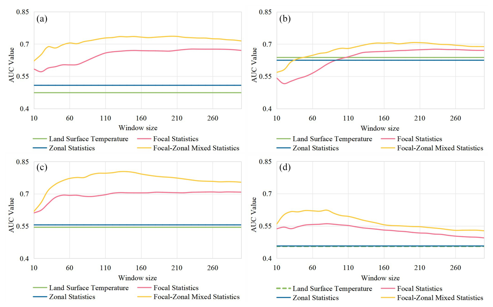
Figure 7 Variations in AUC values with increasing local window radius (measured in pixel units) for land surface temperature (LST) and its three enhancement indices derived from focal statistics, zonal statistics, and focal–zonal mixed statistics. The geothermal wells are represented as circles with an area of 0.035 km² . Panels (a) through (d) correspond to the LST data acquired in the spring, summer, autumn, and winter of 2023, respectively.

Figures S1 and S2 present the modeling results for the years 2015 and 2019, respectively, under the condition that each geothermal well is represented by a circular area of 0.035 km² .

Figures S3 to S5 show the results for the years 2015, 2019, and 2023, respectively, where the representative area for each geothermal well is defined as a single pixel (30 m × 30 m, i.e., 0.0009 km²).

Overall, the two enhancement models incorporating neighborhood windows – focal statistics and focal–zonal mixed statistics – consistently outperform both the zonal statistics model and the original, unenhanced LST. The relatively poor performance of zonal statistics is primarily attributed to the strong spatial variability of LST and the limitations of the simple classification scheme employed. Moreover, since neighborhood-based methods are inherently sensitive to spatial scale, the effectiveness of both focal statistics and focal–zonal mixed statistics varies with changes in window size.

However, regardless of the specific modeling configuration – including different years (2015, 2019, or 2023), seasons (spring, summer, autumn, or winter), definitions of the geothermal well representative area (either a single pixel of 0.0009 km² or a circular area of 0.035 km²), and a wide range of local window sizes (radii from 0.3 to 9 km in 0.3 km intervals) – focal–zonal mixed statistics consistently delivers superior performance compared to focal statistics. This consistent advantage across diverse scenarios and parameter settings clearly demonstrates the robustness and broader applicability of the proposed method.

5.3 Advancements of the toolbox

The FZStats v1.0 toolbox developed in this study not only integrates traditional focal statistics and zonal statistics – addressing SPD and SSH, respectively – but also innovatively implements focal–zonal mixed statistics by combining spatial proximity and environmental similarity, enabling simultaneous handling of both SPD and SSH. This toolbox thus offers a novel and versatile solution for spatial statistical analysis.

To enhance its applicability across diverse scenarios and computing environments, the toolbox provides a variety of parameter-setting interfaces. In terms of neighborhood window configuration, users can select from rectangular, circular, or elliptical windows, with the elliptical option allowing the expression of spatial anisotropy through adjustable parameters. Regarding statistical measures, the toolbox supports traditional metrics such as mean, standard deviation, minimum, and maximum, as well as flexible calculation of arbitrary percentiles to suit specific analytical needs. To optimize memory usage and computational efficiency, FZStats v1.0 supports both raster chunk processing and multi-process operation modes. This design accommodates different hardware capacities and enables efficient parallel processing on multi-core CPUs. Additionally, users can specify a minimum number of cells for valid statistics through the “threshold” parameter, effectively preventing low-precision and unreliable results caused by insufficient sample sizes.

Finally, to improve automation and multitasking efficiency, the toolbox offers a batch processing solution. Users can define processing parameters within a multi-section INI-format configuration file, thus avoiding repetitive manual operations. This functionality supports one-time parameter setup, automatic execution of multiple tasks, parameter reuse, and error tracking, significantly enhancing operational efficiency and reliability.

6 Conclusions

This study developed the FZStats v1.0 toolbox based on Python 3 and QT5, integrating traditional focal statistics, zonal statistics, and the newly proposed focal–zonal mixed statistics. Detailed algorithmic implementations and modeling processes for these methods were presented, and their performance was evaluated through geothermal anomaly detection experiments. The main conclusions are summarized as follows:

• First, the development of focal–zonal mixed statistics is crucial, as it addresses the limitations of traditional focal statistics and zonal statistics, providing a unified solution for simultaneously handling SPD and SSH.

• Second, FZStats v1.0 offers extensive parameter-setting capabilities, supporting flexible configurations of window shapes and statistical measures. Additionally, through adjustable processing options such as raster chunking and multi-processing, the toolbox can maintain efficient performance across a range of computing environments.

• Third, case study analyses demonstrate that focal–zonal mixed statistics significantly enhance the detection of geothermal anomalies compared to conventional zonal and focal statistics methods, with this advantage proving robust across different conditions.

In summary, FZStats v1.0 not only contributes theoretical innovation to spatial statistical methods but also exhibits strong functionality and flexibility in practical applications. It holds considerable promise for geothermal anomaly detection and broader fields requiring integrated spatial statistical solutions.