smash v1.0: a differentiable and regionalizable high-resolution hydrological modeling and data assimilation framework

The smash software is a differentiable and regionalizable framework enabling modular high-resolution hydrological modeling and data assimilation, from catchment to regional and country scales, for water research and operational applications. smash combines various process-based conceptual operators for vertical and lateral flows, which can be hybridized with a descriptor-to-parameter neural network for regionalization. smash features an efficient, differentiable Fortran solver using Tapenade to automatically derive the adjoint model that supports CPU forward–inverse parallel computing and spatially distributed optimization of large parameter vectors thanks to an accurate cost gradient, interfaced in Python using f90wrap. This article presents smash algorithms and their open-source code, documentation, and tutorials. It highlights foundational research, benchmarking on state-of-the-art datasets, and readiness for scientific and operational use. To ensure reproducibility, open-source datasets are used to demonstrate the main functionalities of smash, including parallel computation performances and the application of multiple spatially distributed conceptual model structures over a large catchment sample. These functionalities include uniform or spatially distributed calibration and regionalization by learning the relation between descriptors and parameters. The provided Python tool allows application to any other catchment from globally available datasets. Using CAMELS, as per recent articles, a median Kling–Gupta efficiency (KGE)>0.8 is obtained in local spatially distributed calibration for daily Génie Rural (GR)-like and variable infiltration capacity (VIC)-like model structures at $\mathrm{d}x={\mathrm{1}}^{\prime }{\mathrm{30}}^{\prime \prime }$ (∼3 km) and KGE>0.6 in spatiotemporal validation in a regionalization context. The regionalization of a high-resolution hourly GR-like model structure at dx=500 m over a difficult Mediterranean flash-flood-prone case results in a Nash–Sutcliffe efficiency (NSE)>0.6 in spatiotemporal validation. The proposed differentiable and regionalizable spatially distributed modeling framework is designed for gradient-based variational data assimilation, applicable to initial state (not shown) and parameter estimation at multiple timescales, and is intended for collaborative research and operational applications. Additionally, smash supports the implementation of other differentiable hydrological and hydraulic models, as well as hybrid physics–AI models, further enhancing its versatility and applicability.

1 Introduction

Hydrological models are indispensable tools for understanding the functioning of hydrosystems, flood and low-flow forecasting, sustainable water management and infrastructure design, environmental protection, and adaptation to a changing climate. Indeed, measurements of hydrological responses are not ubiquitously available (e.g., Beven, 2011), while “everywhere relevant” (Bierkens et al., 2015) estimation of hydrological state fluxes is expected. A model is hence needed to extend and predict those quantities of interest based on available data.

High-resolution spatial datasets have become increasingly accessible, often on a global scale, and enable the description of topography–soil–vegetation properties and atmospheric variables. Examples include the ECMWF atmospheric reanalysis version 5 (ERA5) (Hersbach et al., 2020) and Multi-Source Weighted-Ensemble Precipitation (MSWEP) rainfall product (Beck et al., 2019), flow directions IHU (Eilander et al., 2021) from MERIT terrain elevations (Yamazaki et al., 2017), the SoilGrids pedology (Hengl et al., 2017), and daily discharge from Caravan-CAMELS (Kratzert et al., 2023; Addor et al., 2017), which are used hereafter. Such data can be directly exploited by grid-based spatially distributed hydrological models, whose development at “hyper-resolution” (1 km² or finer) is recognized as a “grand challenge for hydrology” to address water problems facing society (Wood et al., 2011; Bierkens et al., 2015).

Hydrological responses result from combined nonlinear vertical and lateral physical processes occurring at multiple scales in the critical zone, and their limited observability (e.g., Beven, 1989; Milly, 1994; Blöschl and Sivapalan, 1995; Refsgaard, 1997; Vereecken et al., 2019) makes hydrological modeling uncertain and difficult (e.g., Liu and Gupta, 2007)). In the absence of directly exploitable first principles in hydrology (e.g., Dooge, 1986), as opposed to flow mechanistic equations in continuous media such as river hydraulics, meteorology, or oceanography, and given the high heterogeneities of continental hydrosystem compartments and the lack of “scale-relevant theories” (Beven, 1987), process-based hydrological models generally include a certain amount of empiricism. This represents an avenue for the fusion of data assimilation (DA) and uncertainty quantification (UQ) with machine learning (ML) and deep learning (DL) techniques to better exploit the informative richness of multi-source data.

The differentiability of the forward numerical model is a key enabler for gradient-based optimization of high-dimensional parameter vectors, for example, in variational data assimilation for 1D or 2D hydraulic models (Monnier et al., 2016; Brisset et al., 2018) or in spatialized hydrology (Castaings et al., 2009; Jay-Allemand et al., 2020). While differentiability may appear unnecessary for simple lumped hydrological models with only a few parameters, where sampling-based calibration or gradient-free methods remain efficient, the situation changes drastically for spatially distributed models involving thousands of parameters. In such high-dimensional settings, exhaustive sampling becomes computationally infeasible. Numerical differentiability enables the computation of accurate gradients of the cost function or model outputs with respect to high-dimensional parameters, thereby facilitating the use of efficient gradient-based optimization methods. This is particularly important when coupling physical models with neural networks requiring accurate gradients, as demonstrated in recent work on learnable regionalization (Huynh et al., 2024b) and internal flux correction (Huynh et al., 2024a), with large-scale evaluations in Huynh et al. (2025). These approaches rely on numerically differentiable solvers and accurate gradients, enabling thousands of parameters to be trained effectively. This perspective aligns with Shen et al. (2023), who emphasize the importance and potential of differentiable modeling in geosciences, highlighting how it can enhance learning, inference, and integration of physical knowledge within hybrid modeling frameworks.

The “resolution–complexity continuum” (Clark et al., 2017) has been explored over the past 5 decades through various modeling approaches, ranging from point-scale processes numerically integrated at larger scales to spatially lumped representations of system responses (Hrachowitz and Clark, 2017). Among the diverse hydrological models and their underlying hypotheses, components generally describe water storage and transfer (e.g., Fenicia et al., 2011) through various combinations and parameterizations of vertical and lateral storage-flux operators. Several model comparison experiments have analyzed differences between various modeling approaches, evaluating performance in terms of streamflow modeling (Perrin et al., 2001; Reed et al., 2004; Duan et al., 2006; Orth et al., 2015) and internal states such as soil moisture (Orth et al., 2015; Bouaziz et al., 2021). Orth et al. (2015) concluded that “added complexity does not necessarily lead to improved performance of hydrological models”. Notably, parsimonious conceptual models, whether lumped or semi-lumped, have performed efficiently in large-sample studies (e.g., the Génie Rural (GR) model in Perrin et al., 2001, GRSD model in De Lavenne et al., 2019, GR and MORDOR models in Mathevet et al., 2020, FUSE models in Lane et al., 2019, and references therein). Large-sample studies have also been undertaken with spatially distributed models, including variable infiltration capacity (VIC) (Mizukami et al., 2017) with a multiscale parameter regionalization (MPR) (Samaniego et al., 2010) or with pixel-wise calibration on global maps of streamflow characteristics (Yang et al., 2019), a gridded version of Hydrologiska Byråns Vattenbalansavdelning (HBV) applied with MPR-like descriptor-to-parameter regressions on a global dataset (Beck et al., 2020), GloFas (Hirpa et al., 2018), National Hydrologic Model (NHM) (Towler et al., 2023), Wflow (Aerts et al., 2022; van Verseveld et al., 2024), and runoff-relevant parameters of Energy Exascale Earth System Model (E3SM) using a surrogate-assisted Bayesian framework (Xu et al., 2022). Differentiable numerical hydrological modeling has made significant progress in recent years (spatially distributed variational data assimilation (VDA) in Castaings et al., 2009; Lee et al., 2012; Jay-Allemand et al., 2020) for large catchment sample studies with hybrid physics–AI, both with lumped approaches (e.g., Feng et al., 2024) and with high-resolution spatially distributed frameworks (Huynh et al., 2024b, 2025). These large-sample studies enable more general and statistically sound analyses of model performances (Andréassian et al., 2009; Gupta et al., 2014), addressing large-scale challenges with consistent methodologies across various scales and conditions.

All hydrological models are inherently conceptual, and calibration or learning is generally required due to limitations and uncertainties in their structure, parameter representativity, data availability, and initial and boundary conditions. These models are typically calibrated and validated using discharge time series at the catchment outlet(s) (Sebben et al., 2013). However, calibrating hydrological model parameters from sparse and integrative discharge data is a challenging inverse problem complicated by equifinality issues (Bertalanffy, 1968; Beven, 1993, 2001), especially for distributed models with a large number of cells and parameters (“curse of dimensionality”). Using spatially uniform parameters may not be the best way to exploit a spatially distributed model (under-parameterization), while fully distributed parameter calibration, which requires a gradient-based approach (Castaings et al., 2009; Lee et al., 2012; Jay-Allemand et al., 2020), faces over-parameterization. Therefore, a parameter regionalization approach using multi-linear descriptor-to-parameter transfer functions has been proposed for distributed models (Beck et al., 2020). More recently, this approach has been advanced with regionalization neural networks (Huynh et al., 2024b) integrated into the differentiable spatialized smash model (Colleoni et al., 2022), which is the focus of the present article, introducing a new numerical code and conducting original tests on a large sample of catchments with open-source data. This approach also enables learning via cost functions based on hydrological signatures, which are obtained using automatic signal analysis algorithms applicable to large samples with smash (Huynh et al., 2023).

This article presents the computational framework smash dedicated to Spatially distributed Modeling and ASsimilation for Hydrology. The smash framework combines vertical and lateral flow operators, either process-based conceptual or hybrid with neural networks (which allows learning regionalization relations between descriptors and parameters), and performs high-dimensional optimization from multi-source data. It is based on an efficient and automatically differentiable Fortran solver enabling CPU parallel computing, which is interfaced in Python using f90wrap (Kermode, 2020; Jay-Allemand et al., 2022) (https://github.com/jameskermode/f90wrap, last access: 25 July 2025). This open-source smash code, version v1.0 (https://github.com/DassHydro/smash, last access: 25 July 2025), is presented here in terms of mathematical formulation, numerical modeling approach, and functionalities, and full details can be found in our research articles from which this software stems (Colleoni et al., 2022; Huynh et al., 2023, 2024b) and in the online documentation (https://smash.recover.inrae.fr, last access: 25 July 2025). Note that smash has also been developed for operational applications. It is the core solver of the French flash flood forecasting system (Piotte et al., 2020). The proposed framework leverages adjoint-based VDA, enabling the simultaneous inference of high-dimensional and spatially distributed parameters (as illustrated) and initial states (implementation available and tested in smash v1.0 but not shown), applicable at both long and short timescales.

This article is organized as follows. Section 2 describes the smash forward model and the inverse algorithm. In Sect. 3 we describe the smash build system framework, documentation, and computational performance. Some applications of smash are demonstrated in Sect. 4 using open-source datasets, focusing on the contiguous US (CONUS) and on a high-resolution flash-flood-prone case study in France. Section 5 illustrates other aspects of smash not presented in Sect. 4, followed by conclusions in Sect. 6.

2 Model and optimization algorithm description

The smash framework contains various hydrological model structures with varying vertical and lateral flow operators and spatialized routing schemes. It is designed to simulate discharge hydrographs and hydrological states at any spatial location within a structured mesh, and it reproduces the hydrological response of contrasted catchments by taking advantage of spatially distributed meteorological forcings, physiographic data, and hydrometric observations. Cost function gradient maps with respect to tunable parameters are a key feature of smash and can easily be combined to gradients of external operators, such as a regionalization neural network (Huynh et al., 2024b) with a chain rule in the context of high-dimensional optimization.

2.1 Forward model statement

Let Ω⊂ℝ² denote a 2D spatial domain that can contain one to many gauges, with x∈Ω being the spatial coordinate, $t\in \left]\mathrm{0},T\right]$ the physical time, and 𝒟_Ω a drainage plan over Ω. The spatially distributed rainfall–runoff model ℳ is a dynamic operator projecting the input fields of atmospheric forcings 𝓘 onto the fields of surface discharge Q, internal states h, and internal fluxes q, as expressed in Eq. (1):

$$\begin{array}{ll}{\displaystyle }\mathit{U}(x,t)& {\displaystyle }=\left[Q,\mathit{h},\mathit{q}\right]\left(x,t\right)\\ \text{(1)}& {\displaystyle }& {\displaystyle }=\mathcal{M}\left({\mathcal{D}}_{\mathrm{\Omega }};\mathcal{I}(x,t);\left[\mathit{\theta },{\mathit{h}}_{\mathrm{0}}\right]\left(x\right)\right),\end{array}$$

with U(x,t) being the modeled state-flux variables and θ and h₀ being the spatially distributed parameters and initial states of the hydrological model.

The spatially distributed rainfall–runoff model ℳ is obtained by partial composition (each operator taking various other input data and parameters) of the flow operators as follows:

$$\begin{array}{}\text{(2)}& {\displaystyle }{\displaystyle }\mathcal{M}={\mathcal{M}}_{\mathit{\text{hy}}}\left(.,{\mathcal{M}}_{\mathit{\text{rr}}}\left(.,{\mathcal{M}}_{\mathit{\text{snw}}}\right)\right).\end{array}$$

Several process-based conceptual operators are available in smash for composing a model:

• Snow operator ℳ_snw. This optional operator simulates melt flux m_lt(x,t), which feeds the hydrological operator in addition to rain.

  • zero: no module

  • ssn: degree-day module

• Hydrological operator ℳ_rr. The simulation occurs at the pixel scale of elementary runoff q_t(x,t), feeding the routing operator.

  • gr4: GR-like module (Perrin et al., 2003; Mathevet, 2005)

  • gr5: GR-like module (Le Moine, 2008; Ficchì et al., 2019)

  • grd: GR-like module (Perrin et al., 2003; Jay-Allemand et al., 2020)

  • loieau: GR-like module (Perrin et al., 2003; Folton and Arnaud, 2020)

  • vic3l: VIC-like module adapted from Liang et al. (1994)

• Routing operator ℳ_hy. Runoff is routed from pixel to pixel to obtain spatiotemporal discharge Q(x,t).

  • lag0: instantaneous module

  • lr: linear reservoir module

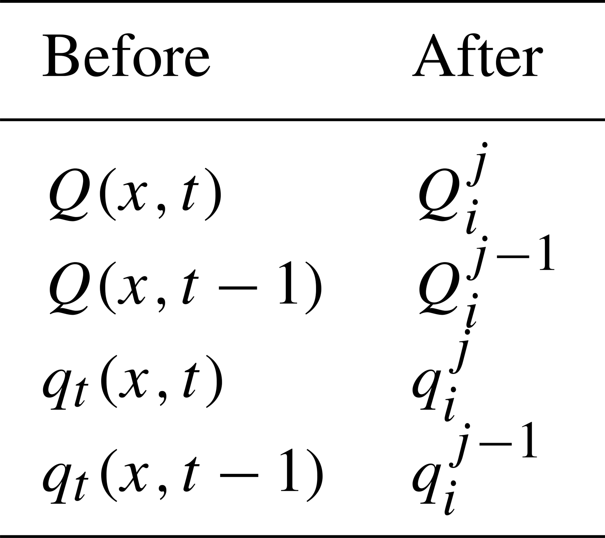
  • kw: kinematic wave module (a classical 1D conceptual kinematic wave model, applied over a D8 drainage plan 𝒟_Ω without channel and solved numerically using a linearized implicit scheme) (Chow et al., 1998).

The operator chaining principle is schematized in Fig. 1 with input data and internal states and fluxes. The operators available in smash are listed above and further detailed in Appendix D and in the online documentation (https://smash.recover.inrae.fr/math_num_documentation/forward_structure.html, last access: 25 July 2025).

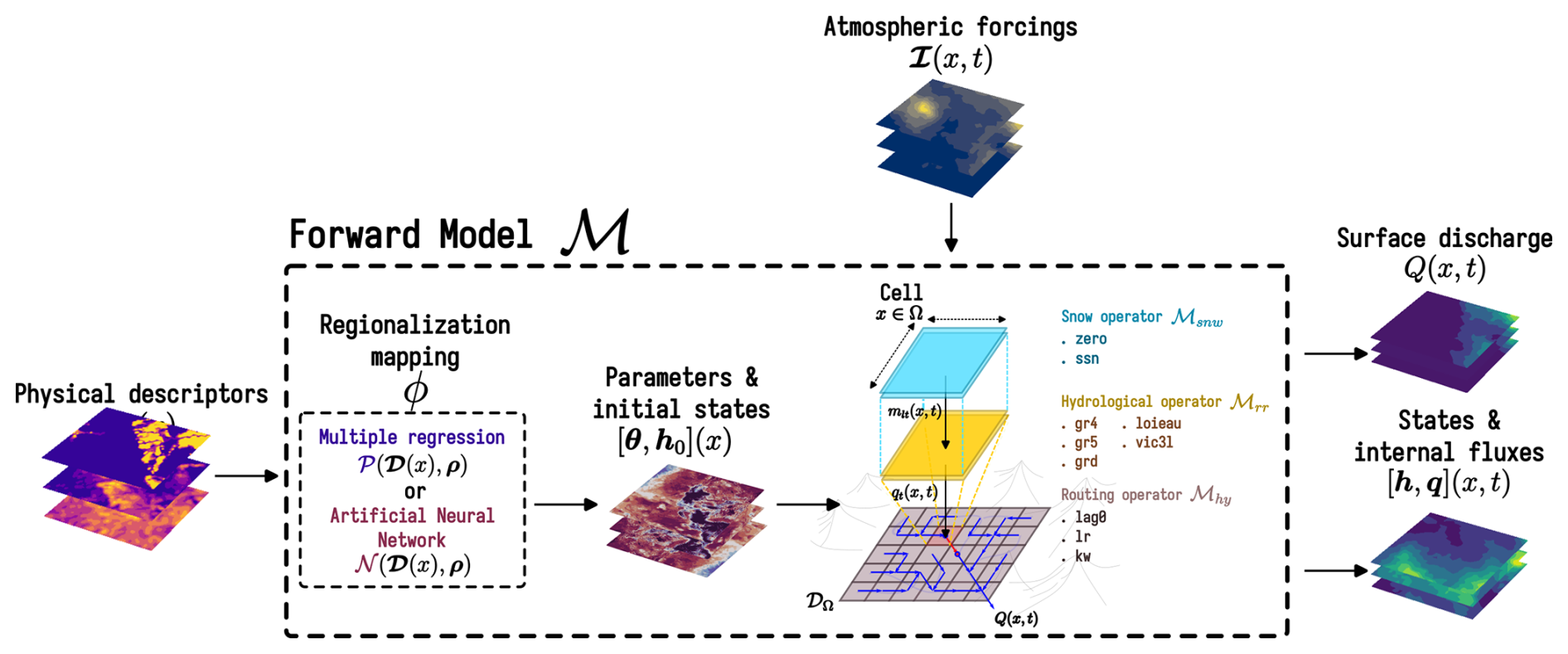
Figure 1 Flowchart of input data, operator chaining to obtain the forward differentiable model ℳ that includes a learnable regionalization mapping ϕ (Huynh et al., 2024b), and simulated states and fluxes. The forward model ℳ is obtained by partial composition (each operator taking various other input data and parameters) of the flow operators $\mathcal{M}={\mathcal{M}}_{\mathit{\text{hy}}}\left(.,{\mathcal{M}}_{\mathit{\text{rr}}}\left(.,{\mathcal{M}}_{\mathit{\text{snw}}}\right)\right)$.

Originally, a differentiable descriptor-to-parameter mapping ϕ can be used to constrain spatially distributed conceptual parameters θ(x) and initial states h₀(x) from physical descriptors D(x) for regionalization learning (Huynh et al., 2024b):

$$\begin{array}{}\text{(3)}& {\displaystyle }{\displaystyle }\left[\mathit{\theta },{\mathit{h}}_{\mathrm{0}}\right]\left(x\right)=\mathit{\varphi }(\mathit{D}\left(x\right),\mathit{\rho }),\forall x\in \mathrm{\Omega },\end{array}$$

with D being the N_D-dimensional vector of physical descriptor maps covering the spatial domain Ω and ρ being the vector of the tunable regionalization parameters of the available mappings (written for θ only for brevity).

1. The first component is a set 𝒫 of multiple regression operators for each parameter of the forward hydrological model ℳ:

   $$\begin{array}{ll}{\displaystyle }{\mathit{\theta }}_k(x,\mathit{D},{\mathit{\rho }}_k)=& {\displaystyle }{s}_k\left({\mathit{\alpha }}_{k,\mathrm{0}}+\sum _{d=\mathrm{1}}^{N_D}{\mathit{\alpha }}_{k,d}{D}_d^{{\mathit{\beta }}_{k,d}}\left(x\right)\right),\\ \text{(4)}& {\displaystyle }& {\displaystyle }\forall k\in \left[\mathrm{1}\mathrm{\dots }{N}_{\mathit{\theta }}\right]\end{array}$$

   where $s_k\left(z\right)=l_k+(u_k-l_k)/\left(\mathrm{1}+e^{-z}\right)$, and $\forall z\in \mathbb{R}$ is a transformation based on a sigmoid function with values in [l_k,u_k] imposing constraints onto the forward model such that $l_k<{\mathit{\theta }}_k\left(x\right)<u_k,\forall x\in \mathrm{\Omega }$. The bounds l_k and u_k associated with each conceptual parameter θ_k are spatially uniform. The regional parameter control vector used for estimation in this case is $\mathit{\rho }\equiv {\left[{\left({\mathit{\rho }}_k\right)}_{k=\mathrm{1}}^{N_{\mathit{\theta }}}\right]}^{\mathrm{T}}\equiv {\left[{\left({\mathit{\alpha }}_{k,\mathrm{0}},{\left({\mathit{\alpha }}_{k,d},{\mathit{\beta }}_{k,d}\right)}_{d=\mathrm{1}}^{N_D}\right)}_{k=\mathrm{1}}^{N_{\mathit{\theta }}}\right]}^{\mathrm{T}}$, and a multiple linear regression mapping is obtained by imposing ${\mathit{\beta }}_{k,d}=\mathrm{1}$.

2. The second component is an artificial neural network (ANN) denoted 𝒩, consisting of a multi-layer perceptron, aimed at learning the descriptor-to-parameter mapping such that

   $$\begin{array}{}\text{(5)}& {\displaystyle }{\displaystyle }\mathit{\theta }(x,\mathit{D},\mathit{\rho })=\mathcal{N}\left(\mathit{D}\left(x\right),\mathit{W},\mathit{b}\right),\forall x\in \mathrm{\Omega },\end{array}$$

   where W and b are the weights and biases of the neural network composed of N_L dense layers respectively. The architecture of the neural network and the forward propagation is detailed in Huynh et al. (2024b). Note that an output layer consisting of a scaling transformation is used to impose bound constraints as above. The regional control vector in this case is $\mathit{\rho }\equiv {\left[\mathit{W},\mathit{b}\right]}^{\mathrm{T}}\equiv {\left[{\left({\mathit{W}}_j,{\mathit{b}}_j\right)}_{j=\mathrm{1}}^{N_L}\right]}^{\mathrm{T}}$.

Note the following:

• The available mappings for ϕ are also implemented to predict the initial state vector h₀ using physical descriptor fields that can include previous states and can be used for short-range data assimilation (not studied here).

• By construction, the complete forward model ℳ is learnable in terms of parameter regionalization, through the regionalization mapping ϕ embedded into ℳ that is also differentiable, and its parameters ρ can be trained using a cost gradient as explained hereafter.

2.2 Inverse algorithm

Given observed and simulated discharge time series ${\mathit{Q}}^{*}=(Q_{g=\mathrm{1}\mathrm{\dots }{N}_G}^{*}{)}^{\mathrm{T}}$ and $\mathit{Q}=(Q_{g=\mathrm{1}\mathrm{\dots }{N}_G}{)}^{\mathrm{T}}$, with N_G being the number of gauges over the study domain Ω, the model misfit to multi-site observations is measured through a cost function J that can be written as

$$\begin{array}{}\text{(6)}& {\displaystyle }{\displaystyle }J({\mathit{Q}}^{*},\mathit{Q})=\sum _{g=\mathrm{1}}^{N_G}{w}_g{j}_g\left(Q_g^{*},Q_g\right)+j_{\text{reg}},\end{array}$$

with w_g being the weight associated with the cost function j_g at each gauge g, where ${\sum }_{g=\mathrm{1}}^{N_g}{w}_g=\mathrm{1}$. This multi-gauge observation cost function is also used for mono-gauge calibration with N_G=1. A regularization term j_reg can be considered for ill-posed inverse problems (Jay-Allemand et al., 2020, 2024). In this study, equal weights were assigned to each gauge (i.e., $w_g=\mathrm{1}/N_G$), which corresponds to minimizing the average of the individual cost functions. Additionally, no regularization term was applied.

The gauge cost function is defined as

$$\begin{array}{}\text{(7)}& {\displaystyle }{\displaystyle }{j}_g(Q_g^{*},Q_g)=\sum _{c=\mathrm{1}}^{N_C}{w}_c{j}_c\left(Q_g^{*},Q_g\right),\end{array}$$

with j_c being based on any efficiency metric (e.g., Nash–Sutcliffe efficiency, NSE; Kling–Gupta efficiency, KGE; Gupta et al., 2009) or a signature-based cost function including N_C continuous and event-based components (Huynh et al., 2023) and w_c being their relative weights. For the multi-score calibration strategy using continuous NSE and event-based flood signatures, see Huynh et al. (2023).

The global cost function J is defined as a convex and differentiable function, involving the response of the forward model ℳ through its output Q, and consequently depends on the model parameters θ and hence on the parameters ρ of the regional mapping ϕ when used (Eq. 3).

Therefore, the optimization problem is formulated as in Eq. (8):

$$\begin{array}{}\text{(8)}& {\displaystyle }{\displaystyle }\widehat{\mathit{\rho }}=\arg \underset{\mathit{\rho }}{min}J\left({\mathit{Q}}^{*},\mathcal{M}(.,\mathit{\varphi }(.,\mathit{\rho }\left)\right)\right).\end{array}$$

This high-dimensional inverse problem can be tackled with gradient-based optimization algorithms. A limited-memory quasi-Newton approach, such as L-BFGS-B (Zhu et al., 1997), is suitable for smooth objective functions, while an adaptive learning rate approach, exemplified by Adam (Kingma and Ba, 2014), is effective for non-smooth objective functions. These approaches necessitate obtaining the gradient ∇_ρJ of the cost function with respect to the tunable control parameter ρ obtained by solving the adjoint D_ρℳ of the forward model ℳ. The adjoint model is obtained by automatic differentiation using the Tapenade engine (Hascoet and Pascual, 2013) (https://team.inria.fr/ecuador/fr/tapenade/, last access: 25 July 2025). The complete forward model and VDA process are illustrated in Fig. 2.

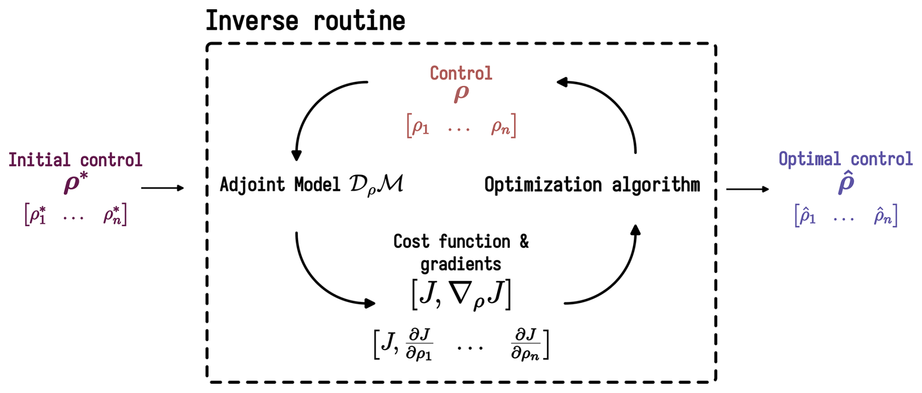
Figure 2 Flowchart of the inverse algorithm that uses the cost gradient ∇_ρJ with respect to the tunable control parameter ρ obtained by solving the adjoint model D_ρℳ of the forward model ℳ, which is obtained by automatic source code differentiation and enabling accurate gradient computation (adapted from VDA course Monnier, 2024).

3 Computational software and performance

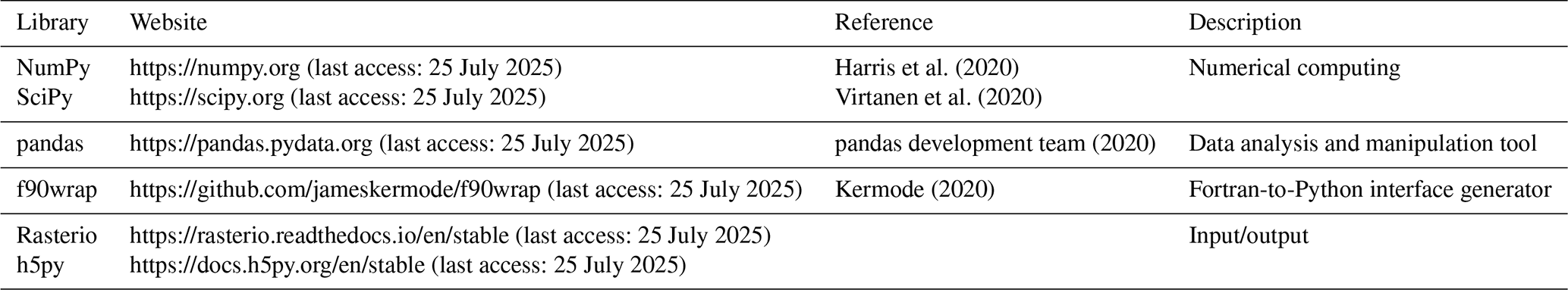
In this section, we focus on code architecture, documentation, and computational performance. smash is based on a computationally efficient Fortran core enabling parallel computations over large domains with OpenMP (Dagum and Menon, 1998) (https://www.openmp.org, last access: 25 July 2025) and is automatically differentiable with the Tapenade engine (Hascoet and Pascual, 2013) to generate the numerical adjoint model. It is interfaced in Python using f90wrap (Kermode, 2020) to provide a user-friendly and versatile interface for quick learning and efficient development and to make the wealth of Python modules and libraries (Table 1) developed by a large and active community directly accessible (data pre-/post-processing, geographic information system, deep learning, etc.).

Harris et al. (2020)Virtanen et al. (2020)pandas development team (2020)Kermode (2020)

Table 1 External Python libraries used by smash.

3.1 From sources to ready-to-use Python library

smash contains a Python core for all user interface functions, both pre- and post-processing, and a Fortran core (with a few C files) for high-performance numerical computations. In order to produce a Python library, including binary files, which can be installed directly from the package manager, PyPI (https://pypi.org, last access: 25 July 2025), several steps are necessary. The first step is to generate the Fortran adjoint file from the Fortran sources. This is done via the Tapenade automatic differentiation engine (Hascoet and Pascual, 2013), which requires the use of Java. Next, the Fortran code is wrapped for use in Python. f90wrap (Kermode, 2020) builds on the capabilities of the popular F2PY (https://numpy.org/doc/stable/f2py, last access: 25 July 2025) utility by generating a simpler Fortran interface to the original Fortran sources, which is then suitable for wrapping with F2PY, together with a higher-level Pythonic wrapper that makes the existence of an additional layer transparent to the final user. The entire build system (except for the generation of the adjoint file, which is external for debugging reasons) is handled by meson (https://mesonbuild.com, last access: 25 July 2025), a multi-platform, multi-language open-source build system that allows us to generate smash binaries on Linux, macOS, and Windows quite easily (Fig. 3).

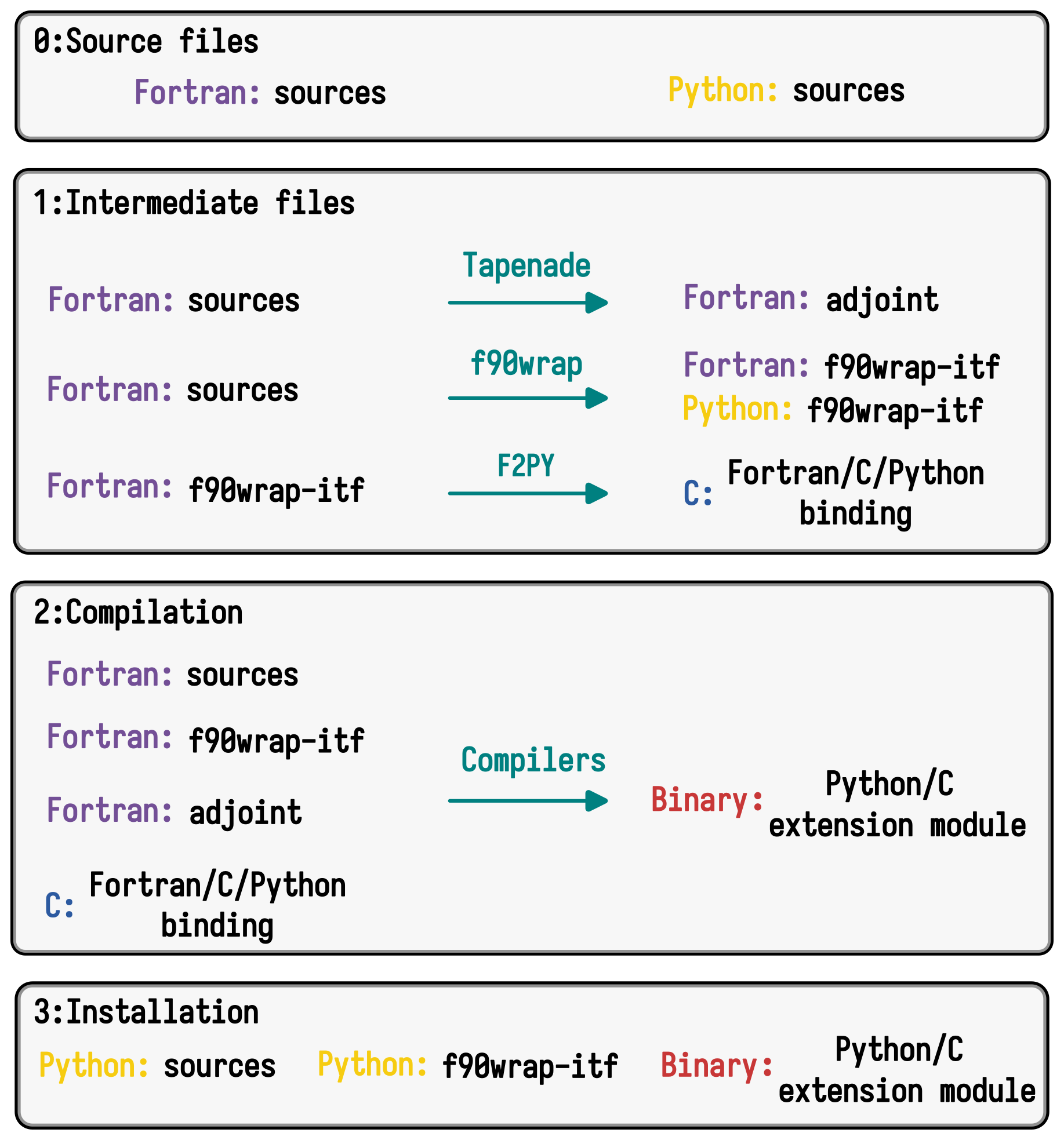
Figure 3 The smash build system framework. It starts with source files written in Fortran and Python (0). In intermediate step (1), Fortran sources are processed by Tapenade to generate the adjoint code and wrapped using f90wrap to create Python interfaces (f90wrap-itf). The F2PY tool is then used to generate a Fortran/C/Python binding from the wrapped interfaces. During compilation step (2), the original Fortran sources, adjoint code, and f90wrap-itf are compiled with appropriate compilers to produce a binary Python/C extension module. Finally, in installation step (3), the Python module is assembled, combining the original Python sources with f90wrap-itf and the compiled binary Python/C extension module, making the high-performance Fortran code accessible from Python.

3.2 Documentation

The smash online documentation (Fig. 4) is divided into four main sections:

• Getting started. This section describes how to install smash from the Python package index PyPI (https://smash.recover.inrae.fr/getting_started, last access: 25 July 2025).

• User guide. This section provides step-by-step examples (and scripts) from basic (simulation run) to complex (regionalization) applications of smash and input data conventions (https://smash.recover.inrae.fr/user_guide, last access: 25 July 2025).

• API reference. This section details the different modules and the application programming interface. Modules are documented using the NumPy-style Python docstring (https://smash.recover.inrae.fr/api_reference, last access: 25 July 2025) .

• Math/num documentation. This last section details the conceptual and mathematical basis of the forward and inverse modeling problems, their numerical resolution, and their optimization and estimation algorithms (https://smash.recover.inrae.fr/math_num_documentation, last access: 25 July 2025).

Figure 4 smash documentation home page accessible at https://smash.recover.inrae.fr (last access: 25 July 2025).

All documentation is implemented using Sphinx (https://www.sphinx-doc.org/en/master, last access: 25 July 2025) to automatically compile and update an online version.

3.3 Computational performance

In this section, we compare the performance of smash in terms of computation time and memory usage between direct and adjoint runs (an adjoint run is equivalent to a single call to the adjoint model D_ρℳ here). The aim is to highlight the resources required to run smash on configurations similar to real cases. We compare smash over three zones, Sardinia, Great Britain/Ireland, and North America, at a spatial resolution of ${\mathrm{1}}^{\prime }{\mathrm{30}}^{\prime \prime }$ ($\sim \mathrm{3}\mathrm{km}\times \mathrm{3}\mathrm{km}$) over a period of 1 year, from 31 July 2010–31 July 2011, randomly chosen at a daily time step. These three zones were chosen simply to provide three zones of variable surface area (Fig. 5). In addition to the three zones, with smash enabling different assemblies of operators, two structures are compared, s1 and s2, representing the simplest (ℳ_snw: zero, ℳ_rr: grd, and ℳ_hy: lag0) and the most complex (ℳ_snw: ssn, ℳ_rr: vic3l, and ℳ_hy: kw) structures in terms of the number of operations per cell respectively. All the simulations (1 year of simulation at a daily time step) were run on a server with AMD EPYC 7643 CPUs (Appendix E) and 255 GB of RAM.

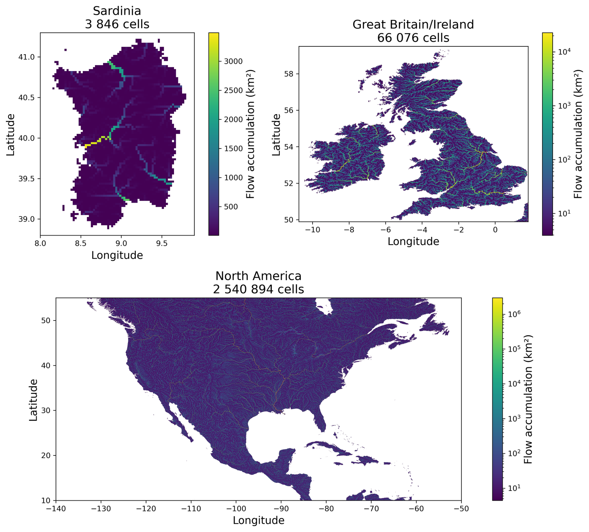
Figure 5 Spatial representations of the three different geographical regions used in the performance benchmarks.

The range of computation times across all simulations (Fig. 6) varies from approximately 0.1 s for a direct run with eight threads in the Sardinia region using the s1 structure to just over an hour for an adjoint run with one thread in the North America region using the s2 structure. Systematically, regardless of the region, number of threads, or type of run, the difference in computation time between the s1 and s2 structures is about a factor of 2. Regarding the differences between a direct run and an adjoint run, the computation time factor varies depending on the number of threads, ranging from a factor of 12 for 1 thread to a factor of 6 for 16 threads. This difference highlights better thread scaling for the adjoint run, with a speedup of around 4 for a direct run and 7 for an adjoint run with 16 threads, likely because the adjoint run is more computationally demanding than the forward run. It is worth noting that in the case of the Sardinia region, which has the fewest grid cells, thread scaling is poor compared to the other two regions, even reaching the limit where thread overhead increases the computation time. Although the time-stepping loop cannot be parallelized, and the routing scheme in smash must be solved sequentially from upstream to downstream, allowing only partial parallelization over the entire spatial domain, the approach still offers a substantial reduction in computation time.

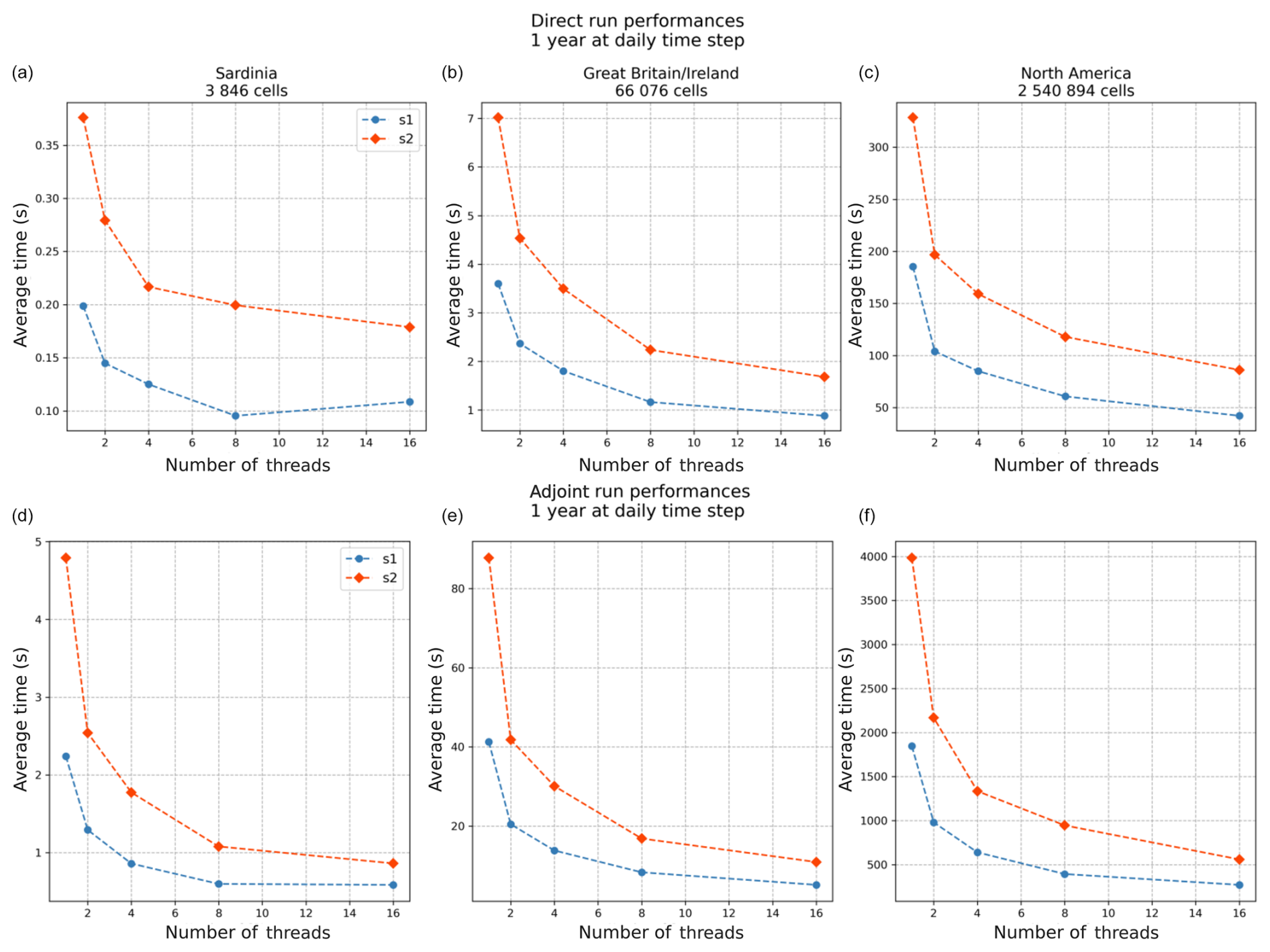
Figure 6 Benchmarking results for both direct (a–c) and adjoint (d–f) run simulations over a period of 1 year at a daily time step, using varying numbers of threads (from 1 to 16). Each plot corresponds to a different geographical region: Sardinia, Great Britain/Ireland, and North America from left to right.

Regarding memory usage (Table 2), values range from 0.17 GB for a direct run in the Sardinia region with the s1 structure to 27 GB for an adjoint run in the North America region with the s2 structure. Systematically, memory usage is higher in the adjoint run than in the direct run and scales with the size of the domain. The main contributor to memory usage in the adjoint run is the forward sweep, which includes a time-stepping loop where iteration n depends on the results of previous iterations. The memory allocation during the forward sweep is freed during the backward sweep, but it still results in a significant memory peak. This memory peak has been considerably reduced in the smash version presented here by including checkpoints within the time-stepping loop. These checkpoints allow us to alternate between forward and backward sweeps, leading to much smaller memory peaks compared to a single sweep. The downside of using checkpoints is the increase in computation time, but this was considered less significant compared to the memory saving (see Hascoet and Pascual, 2013, for further details about forward and backward sweeps and checkpointing).

Table 2 Memory usage in gigabyte (GB) for both direct and adjoint run simulations over a period of 1 year at a daily time step.

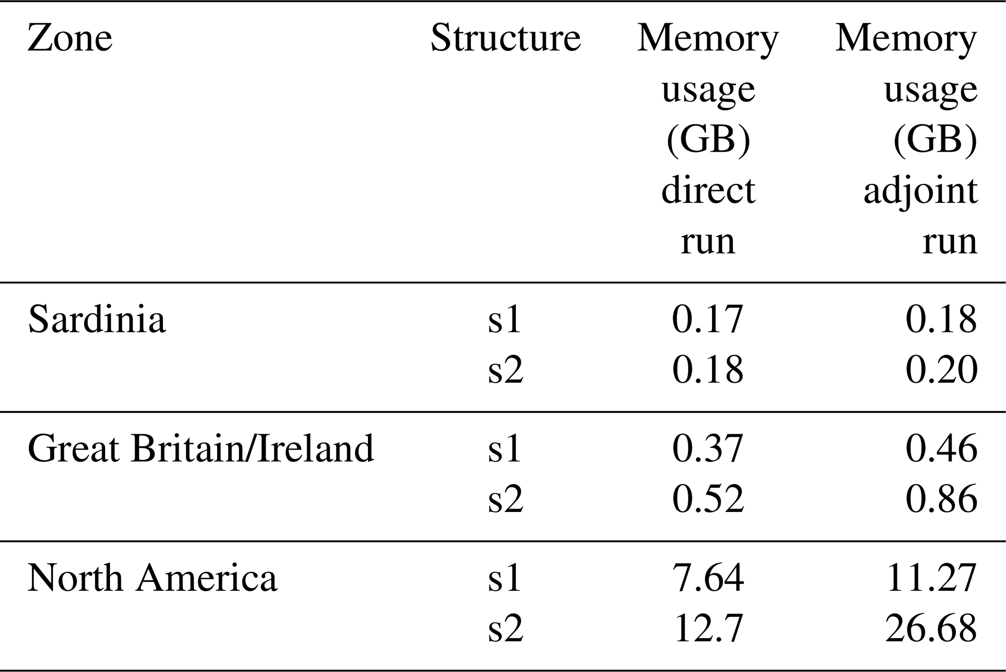
In conclusion, these computation times and memory usage demonstrate the feasibility of the model for large-scale applications. The critical point is parameter estimation. In the case of parameter estimation using a gradient-based optimizer, one or more adjoint runs are evaluated at each iteration, significantly multiplying the total computation time. As an example, Huynh et al. (2024b) performed a calibration at a spatial resolution of 1 km over a domain of more than 20 000 cells and at a temporal resolution of 1 h over a period of 4 years. The calibration required 350 calls to the adjoint model, resulting in a computation time of around 180 h. Currently, memory usage in the adjoint run is less of a limiting factor than computation time for large-domain applications. Thus, further improving computation time is a priority to expand the model's application to finer spatial and temporal scales.

4 Applications

4.1 Numerical experiments presented

The main functionalities and operators of smash are illustrated in open-source global datasets over the contiguous US (CONUS) (Table 3, Fig. 7) and in a higher-resolution open-source regional dataset in France (Table 4, Fig. 7). Models in CONUS will be at a spatial resolution of ${\mathrm{1}}^{\prime }{\mathrm{30}}^{\prime \prime }$ ($\sim \mathrm{3}\mathrm{km}\times \mathrm{3}\mathrm{km}$) and daily time step, while higher-resolution models will be set up in France at 500 m spatial resolution and an hourly time step. The numerical results presented are as follows:

• split-sample temporal cross-validation of different model structure combinations over CONUS (Sect. 4.2)

• regionalization over CONUS (Sect. 4.3)

• high-resolution regionalization over the Aude River in France (Sect. 4.4).

(Beck et al., 2019)(Beck et al., 2019)(Oudin et al., 2005)(Hersbach et al., 2020)(Hersbach et al., 2020)(Eilander et al., 2021)(Yamazaki et al., 2017)(Hengl et al., 2017)(Hengl et al., 2017)(Beck et al., 2019)(Oudin et al., 2005)(Hersbach et al., 2020)(Beck et al., 2019)(Hersbach et al., 2020)Kratzert et al., 2023Addor et al., 2017

Table 3 Model input data from open-source databases available worldwide used over CONUS: atmospheric forcings $\mathcal{I}=\mathit{\{}\mathit{P},\mathit{N},\mathit{E},\mathit{T}\mathit{\}}$, flow direction map 𝒟_Ω, physical descriptors $\mathit{D}=\mathit{\{}{d}_{\mathrm{1}},\mathrm{\dots },d_{\mathrm{6}}\mathit{\}}$ for regionalization based on the Beck et al. (2020) study, and discharge time series Q^*. The liquid and solid precipitation, P and N, derived from the Multi-Source Weighted-Ensemble Precipitation (MSWEP) (Beck et al., 2019), is divided into liquid and solid parts using a parametric S-shaped curve (Garavaglia et al., 2017) and is disaggregated from 0.1 to 0.025°. The temperature and potential evapotranspiration, T and E, derived from ERA5 (Hersbach et al., 2020), are disaggregated from 0.25 to 0.025°, using the Oudin formula (Oudin et al., 2005) to obtain the potential evapotranspiration. The flow direction, 𝒟_Ω, from MERIT Hydro IHU (Eilander et al., 2021), was upscaled from 0.008 to 0.025° using pyflwdir (https://github.com/Deltares/pyflwdir, last access: 25 July 2025) (Eilander, 2023). The topographic slope, d₁, is derived from MERIT DEM (Yamazaki et al., 2017), upscaled from 0.008 to 0.025° using the gdaldem slope (https://gdal.org/en/latest/programs/gdaldem.html, last access: 25 July 2025). The sand and clay content, d₂ and d₃, from SoilGrids (Hengl et al., 2017), was upscaled and reprojected from 250 m to 0.025°. The meteo-climatic data, d₄, d₅, and d₆, are derived from P and E. The discharge time series, Q^*, comes from Caravan-CAMELS (Kratzert et al., 2023; Addor et al., 2017).

(Champeaux et al., 2009)(Oudin et al., 2005)(Quintana-Seguí et al., 2008; Vidal et al., 2010)(Leblois and Sauquet, 1999)(Leblois and Sauquet, 1999)Organde et al. (2013)

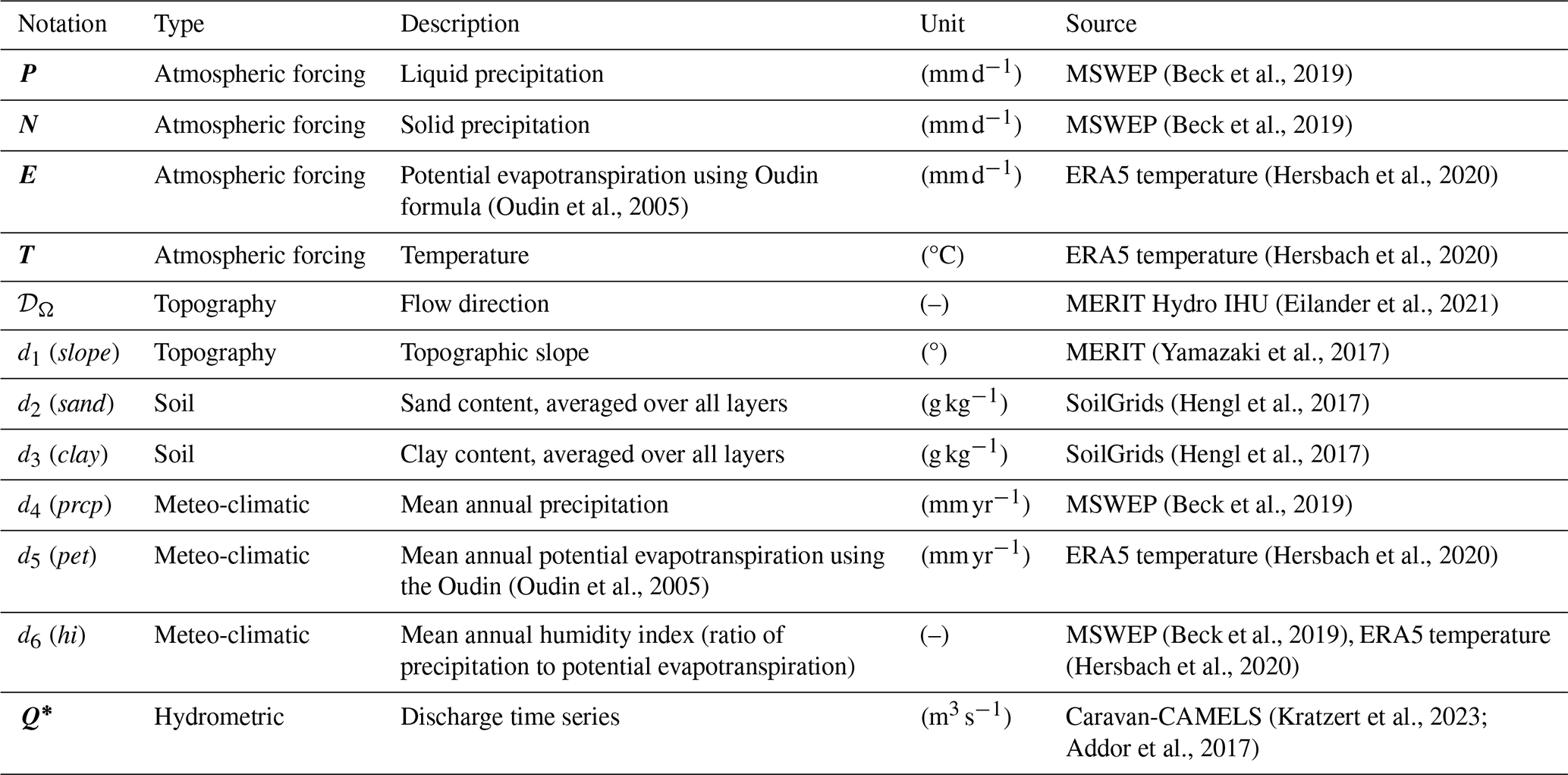
Table 4 Model input data from national open-source databases used over the Aude River in France: atmospheric forcings $\mathcal{I}=\mathit{\{}\mathit{P},\mathit{E}\mathit{\}}$, flow direction map 𝒟_Ω, physical descriptors $\mathit{D}=\mathit{\{}{d}_{\mathrm{1}},\mathrm{\dots },d_{\mathrm{7}}\mathit{\}}$ for regionalization, and discharge time series Q^*. The liquid precipitation, P, comes from the ANTILOPE J+1 Météo-France product (Champeaux et al., 2009), a radar–gauge reanalysis disaggregated from 1 km to 500 m. The potential evapotranspiration, E, is derived from the SAFRAN Météo-France temperature (Quintana-Seguí et al., 2008; Vidal et al., 2010) disaggregated from 8 km to 500 m, using the Oudin formula (Oudin et al., 2005) to obtain daily interannual potential evapotranspiration. The flow direction, 𝒟_Ω, comes from HydroDem (Leblois and Sauquet, 1999). The land cover data, d₁, d₂, d₃, and d₄, are derived from CORINE Land Cover 2018 (https://doi.org/10.2909/71c95a07-e296-44fc-b22b-415f42acfdf0, last access: 25 July 2025), rasterized at 50 m and upscaled to 500 m using the average resampling method. The topographic slope, d₅, is derived from the HydroDem DEM (Leblois and Sauquet, 1999) using the gdaldem slope. The drainage density, d₆, comes from Organde et al. (2013), representing the number of cells crossed by a river. The percentage of karst, d₇, comes from BDLISA (https://bdlisa.eaufrance.fr, last access: 25 July 2025), rasterized at 50 m and upscaled to 500 m using the average resampling method. The discharge time series, Q^*, comes from the HydroPortail Service Central Vigicrues (https://hydro.eaufrance.fr, last access: 25 July 2025).

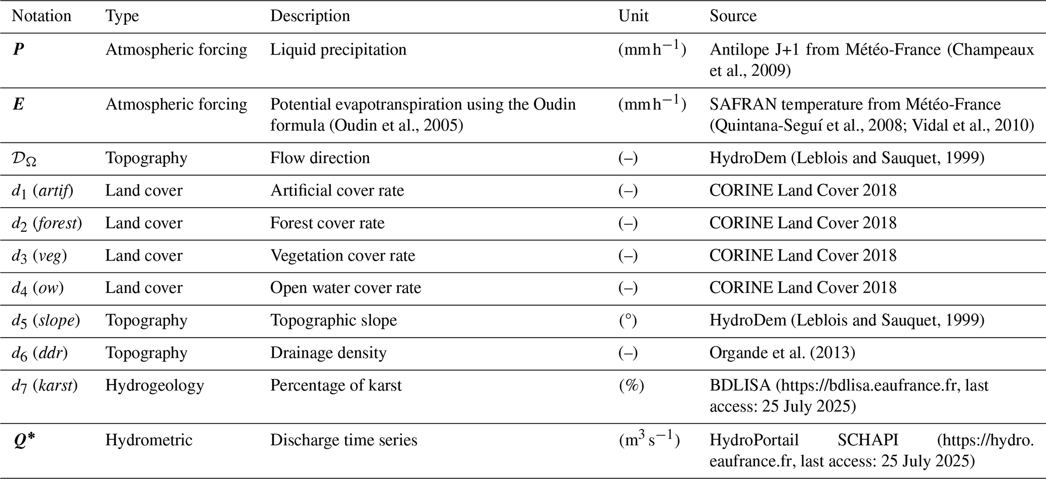
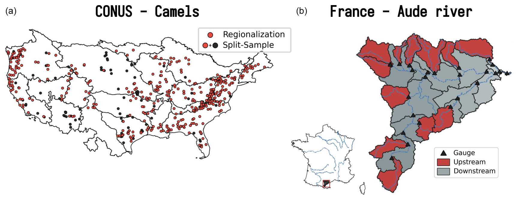
Figure 7 Location of the catchments for the CONUS (a) and France (b) applications. For the split-sample test over CONUS, all 482 catchments from the CAMELS dataset (Addor et al., 2017) are used (orange and black circles), whereas for the regionalization, a subset of 398 catchments is used (only orange circles), removing catchments whose performance is less than 0.75 KGE from local calibration. For the France application over the Aude River, a set of 25 sub-catchments is used for regionalization, with 12 upstream catchments (red-shaded regions) and 13 downstream catchments (gray-shaded regions).

4.2 CONUS – CAMELS: split-sample temporal cross-validation

4.2.1 Numerical experiment settings

A set of 482 catchments (Fig. 7) is modeled with the following experimental design:

• A set of hydrological models is considered, including four GR-like structures (Perrin et al., 2003) (ℳ_rr: gr4, gr5, grd, loieau) and one VIC-like structure (Liang et al., 1994) (ℳ_rr: vic3l). The way in which these models are integrated into smash, which differs from the original models, is described in the documentation (https://smash.recover.inrae.fr/math_num_documentation/forward_structure.html, last access: 25 July 2025) in the forward structure section. For each hydrological model, the same snow module (ℳ_snw: ssn) and routing module (ℳ_hy: kw) are used. A description of the calibrated parameters is provided in Appendix A.

• A split-sample temporal validation procedure (Klemeš, 1983) is set up, splitting the time window covered by hydrometric data into two complementary subsets over sub-periods of 7 years: p1 (from 1 August 2000 to 31 July 2007) and p2 (from 1 August 2007 to 31 July 2014) are both used for calibration and validation. For each period, the 10 preceding years are used as model “warm-up”.

• Two calibration mappings on each catchment are tested, including spatially uniform parameters (gradient-free optimization) and spatially distributed parameters (gradient-based optimization).

• A single-gauge cost function based on the KGE ($J=\mathrm{1}-\text{KGE}$) is used.

4.2.2 Results

The performance of the models resulting from the spatially uniform or distributed calibration is evaluated using the Kling–Gupta efficiency (KGE) for both the calibration and the validation in period p2 only for brevity in this software article (Fig. 8). Overall, performance is satisfactory, with a median between 0.8 and 0.87 for KGE over the calibration period and between 0.72 and 0.78 for KGE over the validation period. With regard to the calibration method, for any model, calibration and validation performances are better with a spatially distributed calibration. This is an expected result for the calibration period, given that spatially distributed calibration is over-parameterized and offers the maximum level of flexibility in the search for the optimal set of parameters, unlike spatially uniform calibration, which is under-parameterized, imposing a single parameter set for each catchment. However, despite this over-parameterization with calibration of spatially distributed parameters, which can lead to over-fitting over the calibration period, the models offer good performance in temporal validation. The differences between the structures are mainly explained by (i) the varying levels of model complexity, two parameters for the grd model and four for the gr5 model, and (ii) the expert knowledge of the different models, which influences, among other things, the choice of initial values, bounds, and parameters to be optimized. The smash historical development based on the GR-like models led to much more substantial expert knowledge than for the VIC-like model recently implemented. Summary statistics of the calibrated parameters are provided in Appendix A.

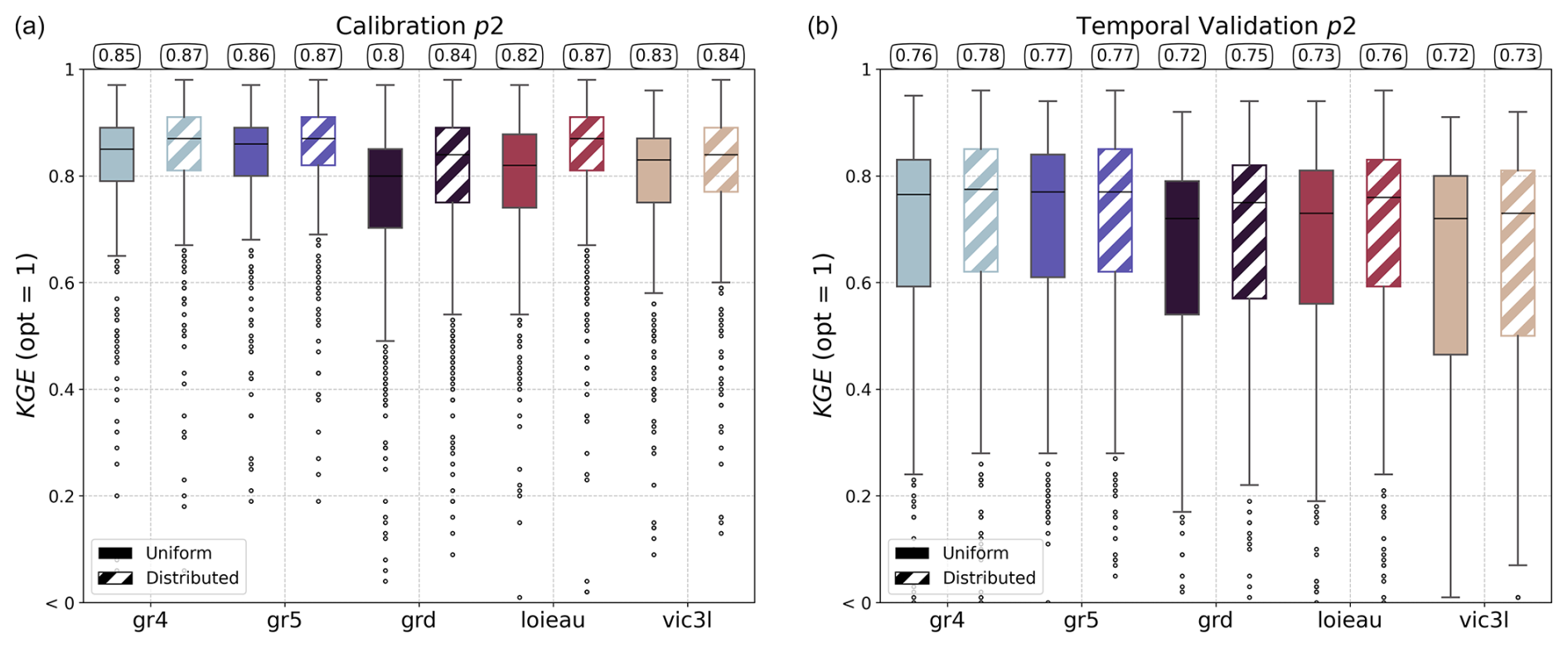
Figure 8 Comparison of the Kling–Gupta efficiency (KGE) performance of different smash hydrological models under spatially uniform and distributed calibration. The models evaluated include gr4, gr5, grd, loieau, and vic3l. Panel (a) shows results for the calibration, while panel (b) displays results for temporal validation in period p2. For each model, results are shown for spatially uniform (solid boxes) and spatially distributed (hatched boxes) calibrations, with the median value highlighted at the top of the boxplot.

Concerning the spatial distribution of KGE values (Fig. 9), the results for the gr4 hydrological model after a spatially distributed calibration show that the best performances are located over the east and west sides of CONUS, while the worst performances are located over the Great Plains area. This spatial pattern of hydrological model performance has also been obtained in other studies (Newman et al., 2015; Beck et al., 2016; Mizukami et al., 2017).

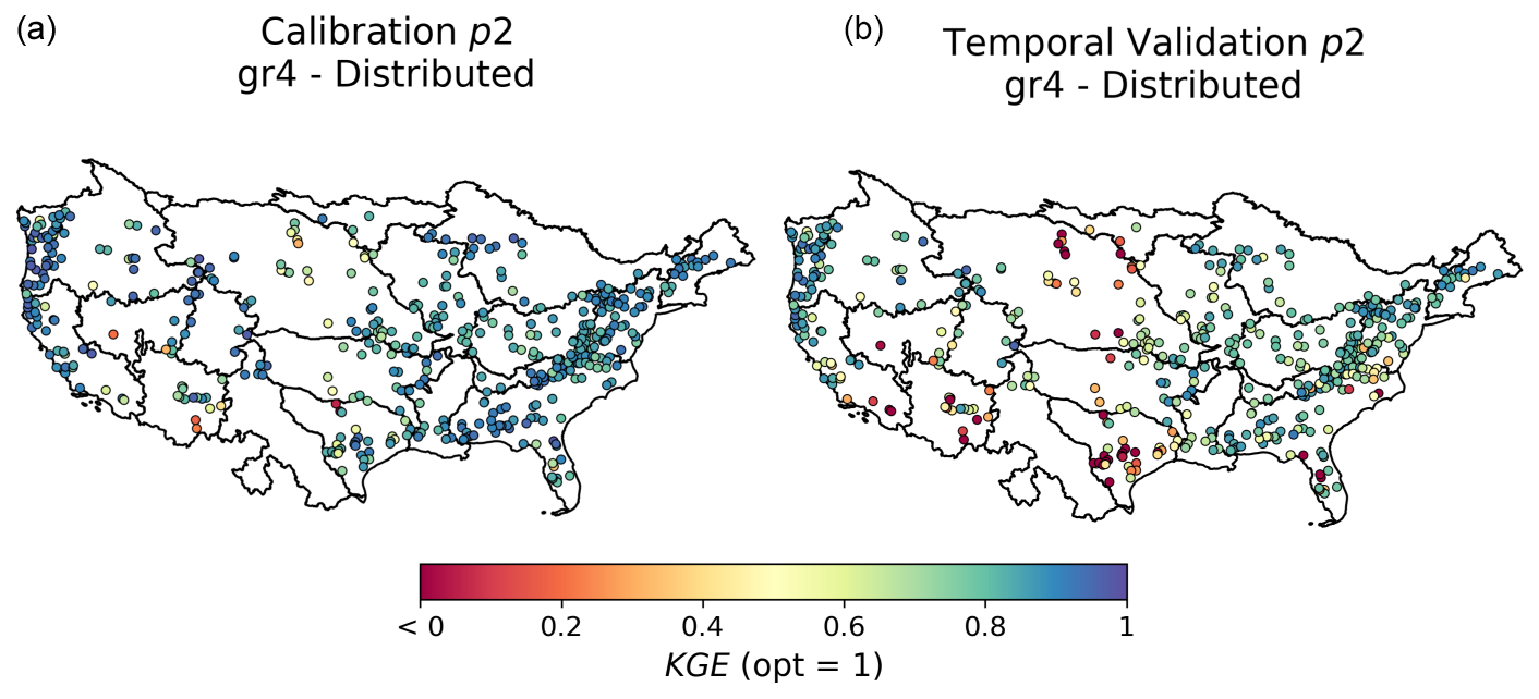
Figure 9 Spatial distribution of the Kling–Gupta efficiency (KGE) scores across different catchments for the gr4 model under local calibration with spatially distributed parameters. Panel (a) shows KGE scores during the calibration period, while panel (b) shows results for temporal validation, using the p2 period.

4.3 CONUS – CAMELS: regionalization

4.3.1 Numerical experiment settings

A set of 398 catchments (Fig. 7) from the CAMELS dataset (Addor et al., 2017) is evaluated in a regionalization context at a spatial resolution of ${\mathrm{1}}^{\prime }{\mathrm{30}}^{\prime \prime }$ and at a daily time step using worldwide databases (Table 3). The experimental design is as follows:

• A subset of catchments from Sect. 4.2 is selected, eliminating catchments where KGE<0.75 from local calibration. This selection is made in order to avoid introducing catchments whose performance could greatly degrade the calibration metric in a multi-gauge context.

• One hydrological model is considered, which is identical to the gr4 model in Sect. 4.2 with the same snow and routing module (ℳ_snw: ssn, ℳ_rr: gr4, and ℳ_hy: kw). A description of the calibrated parameters is provided in Appendix B.

• A spatiotemporal validation procedure is set up by the following:

  • splitting the time window covered by hydrometric data into two complementary subsets over sub-periods of 7 years: p1 (from 1 August 2000 to 31 July 2007) and p2 (from 1 August 2007 to 31 July 2014), with p1 used as the calibration period and p2 as the validation period (for each period, 10 years is used as model “warm-up”);

  • randomly splitting the catchment set into four groups, calibrating on three of the groups with the fourth group held out and used for validation, and then rotating them such that each group is used for validation once.

• Three calibration mappings across the whole CONUS are tested:

  • Uniform. Spatially uniform parameters (gradient-free optimization) are used.

  • Multi-linear. Multiple linear regression is used as a transfer function from descriptors to spatialized parameters (gradient-based optimization).

  • ANN. A multi-layer perceptron composed of three hidden layers is used as a transfer function from descriptors to spatialized parameters (gradient-based optimization).

• A multi-gauge cost function is used based on the average KGE of the calibrated catchments ($J=\frac{\mathrm{1}}{N_G}{\sum }^{N_G}\mathrm{1}-\text{KGE}$).

• A final calibration is performed over the total period p1+p2, including all gauges with the ANN mapping and the same multi-gauge cost function used to analyze the output model parameters and their correlations with input descriptors.

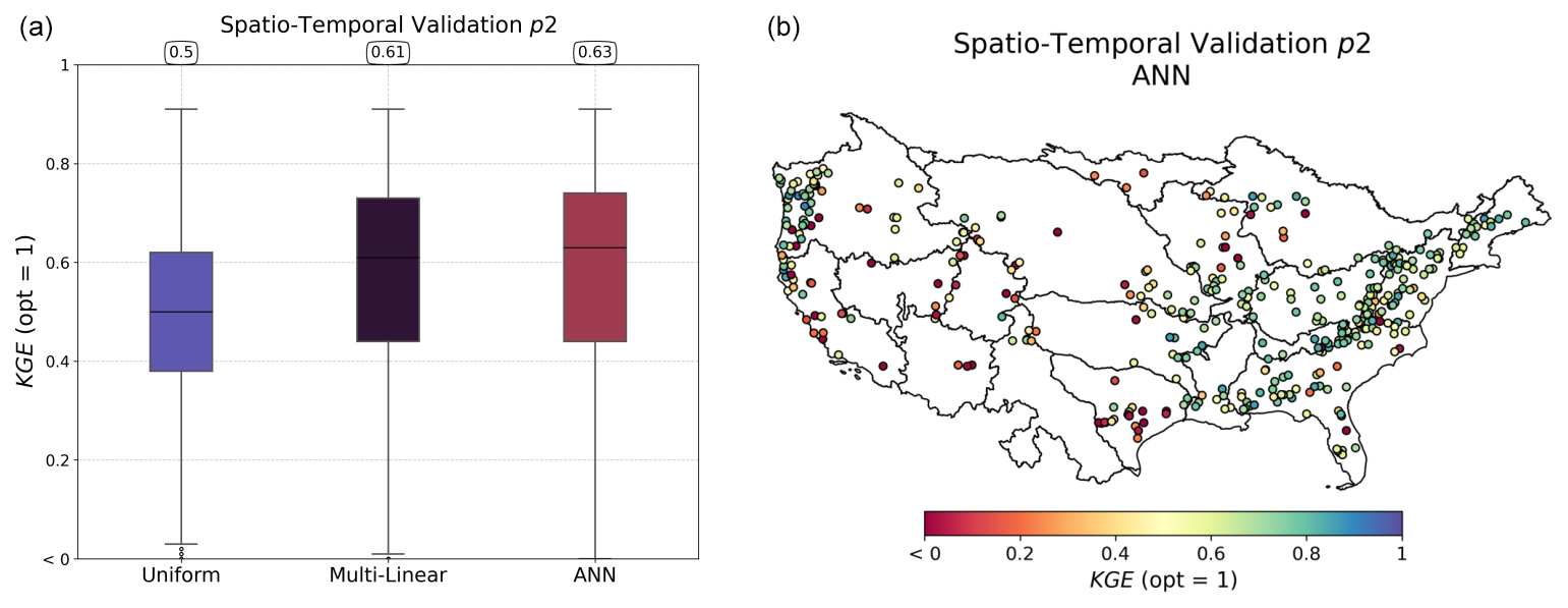
Figure 10 Spatiotemporal validation performance over period p2. The boxplots in panel (a) represent the distribution of Kling–Gupta efficiency (KGE) scores for three calibration methods: uniform, multi-linear, and artificial neural network (ANN). Median values are displayed at the top of each boxplot. The map in panel (b) illustrates the spatial distribution of the KGE values for the ANN mapping across different catchments.

4.3.2 Results

The regional calibration over the CAMELS dataset was performed on four groups of randomly selected catchments, as explained above. The performances in the spatial and/or temporal validation are shown in Fig. 10 and detailed by catchment group in Table B2 for the ANN mapping, which is the best performer. In the spatiotemporal validation, the most challenging extrapolation case, a uniform mapping leads to a median KGE of 0.5, while the two regionalization methods result in a KGE of 0.61 or 0.63 respectively for multi-linear and ANN mapping. These fairly good performances, obtained with a relatively simple setup in terms of descriptors and cost function in particular, are comparable with regionalization works in the literature (Mizukami et al., 2019; Beck et al., 2020; Feng et al., 2024). In a manner similar to the previous section (Sect. 4.2), the worst performances are found in the Great Plains and, more clearly than in the local calibrations, in the western part of the country.

Following the evaluation of performance in spatiotemporal validation, a regional calibration with the ANN mapping over the period including p1 and p2 and with all gauges is carried out. This calibration enables us to analyze the correlations between the physiographic descriptors and the parameters obtained (Fig. 11) in a more robust way than with the various spatiotemporal validation groups. The correlation matrix highlights significant linear correlations, notably between the melt coefficient (k_mlt) and the topographical slope (d₁), the size of the production reservoir (c_p) and the mean annual rainfall (d₄), and the moisture content (d₆) and the routing parameters (a_kw, b_kw) with the same moisture content (d₆). Conversely, the exchange parameter (k_exc), a parameter directly affecting the model's mass balance in a non-conservative way, shows almost no linear correlation with the descriptors and is almost spatially uniform over the whole domain around the value of 0. While a detailed regionalization study on CAMELS datasets using our original adjoint-based algorithms is beyond the scope of this software article, the achieved performance across this large sample already showcases the algorithm's potential for global applicability. It also demonstrates the algorithm's effectiveness in enforcing spatially distributed hydrologic model constraints at the pixel scale, leading to seamless parameter maps at a reasonable computational cost. Regarding computation times, the calibration with ANN mapping over periods p1 and p2 took 95 h. This calibration involved 350 iterations, corresponding to 350 calls to the adjoint model, and was performed using 16 threads. For comparison, a single adjoint model run takes approximately 16 min, whereas a direct model run takes around 5 min using the same number of threads.

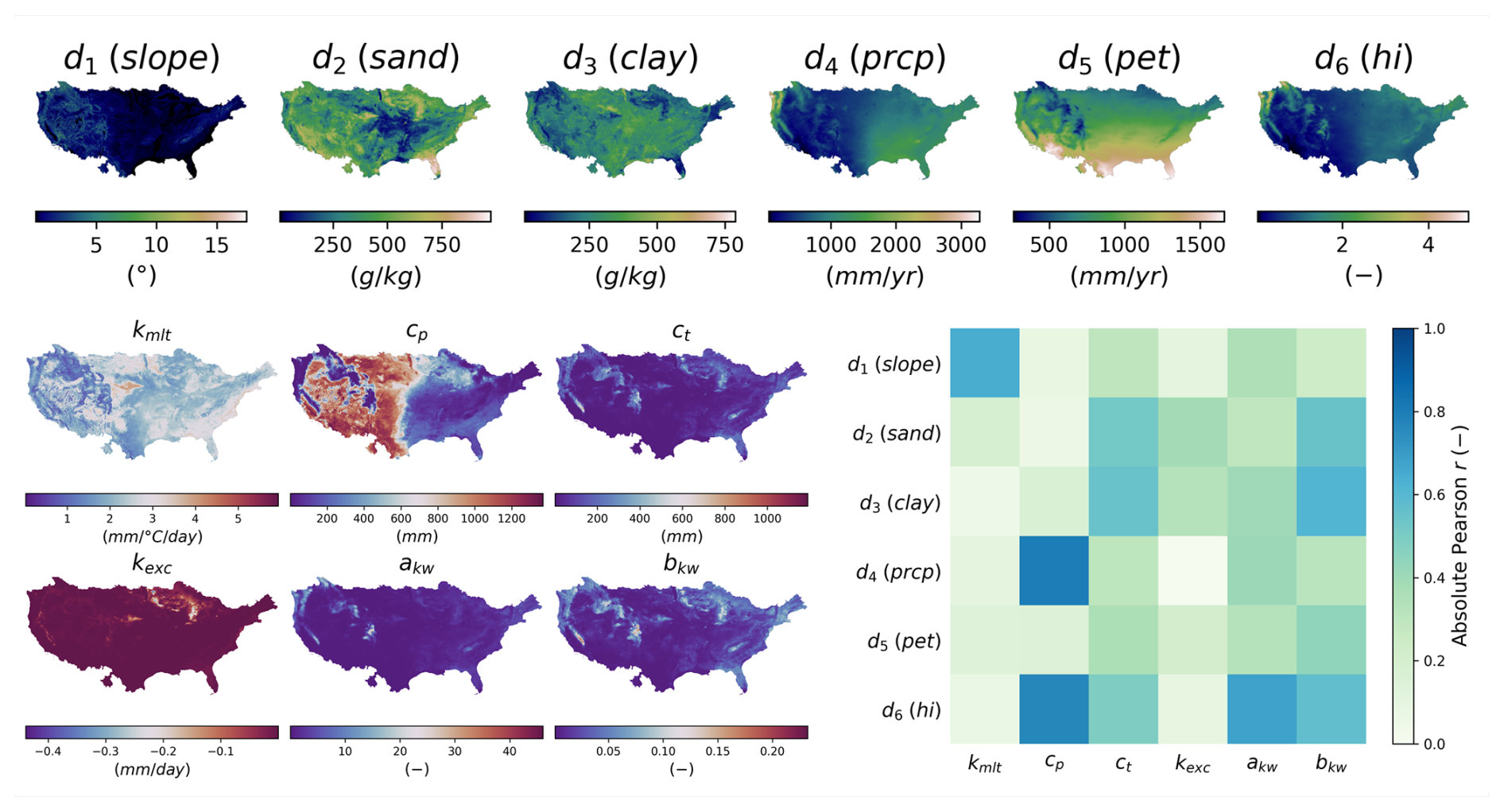
Figure 11 Analysis of input descriptors and output model parameters for the ANN mapping. Spatial distribution of physical descriptors (d₁–d₆) in the top panel, with details provided in Table 3. Spatial distribution of calibrated hydrological parameters (k_mlt, c_p, c_t, k_exc, a_kw, b_kw) in the lower-left panel and linear correlation between descriptors and parameters in the lower-right panel.

Finally, leveraging the fully distributed nature of smash, regional streamflow maps can be generated. An example is shown in Fig. 12, which illustrates the dynamics of Hurricane Katrina over a 6 d period from 27 August to 1 September 2005. Notably, the routing model used in this exercise, the kinematic wave, was applied uniformly across the entire domain, including areas outside its validity range, such as downstream of major rivers on flat topography. Further work focuses on enriching smash with hydraulic models, starting with a 1D and 2D dynamic wave model that neglects the convective acceleration term but retains local acceleration and pressure gradient terms (Bates et al., 2010) for numerical implementation simplicity. Additionally, physics-based differential equations for hydrologic water balance at the pixel scale will be incorporated. Hybrid physics–AI formulations, which embed neural networks capable of learning parameterization and potentially uncertain model operators from data, can be explored thanks to the differentiable nature of the models within smash.

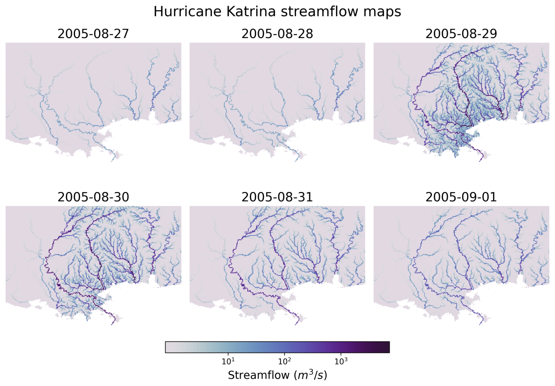
Figure 12 Streamflow dynamics during Hurricane Katrina from 27 August to 1 September 2005 for the ANN mapping. Each panel depicts the streamflow distribution across the affected region. To visualize the temporal evolution of the spatialized discharge pattern, note that the kinematic wave routing was applied on flat topography, i.e., out of its validity range.

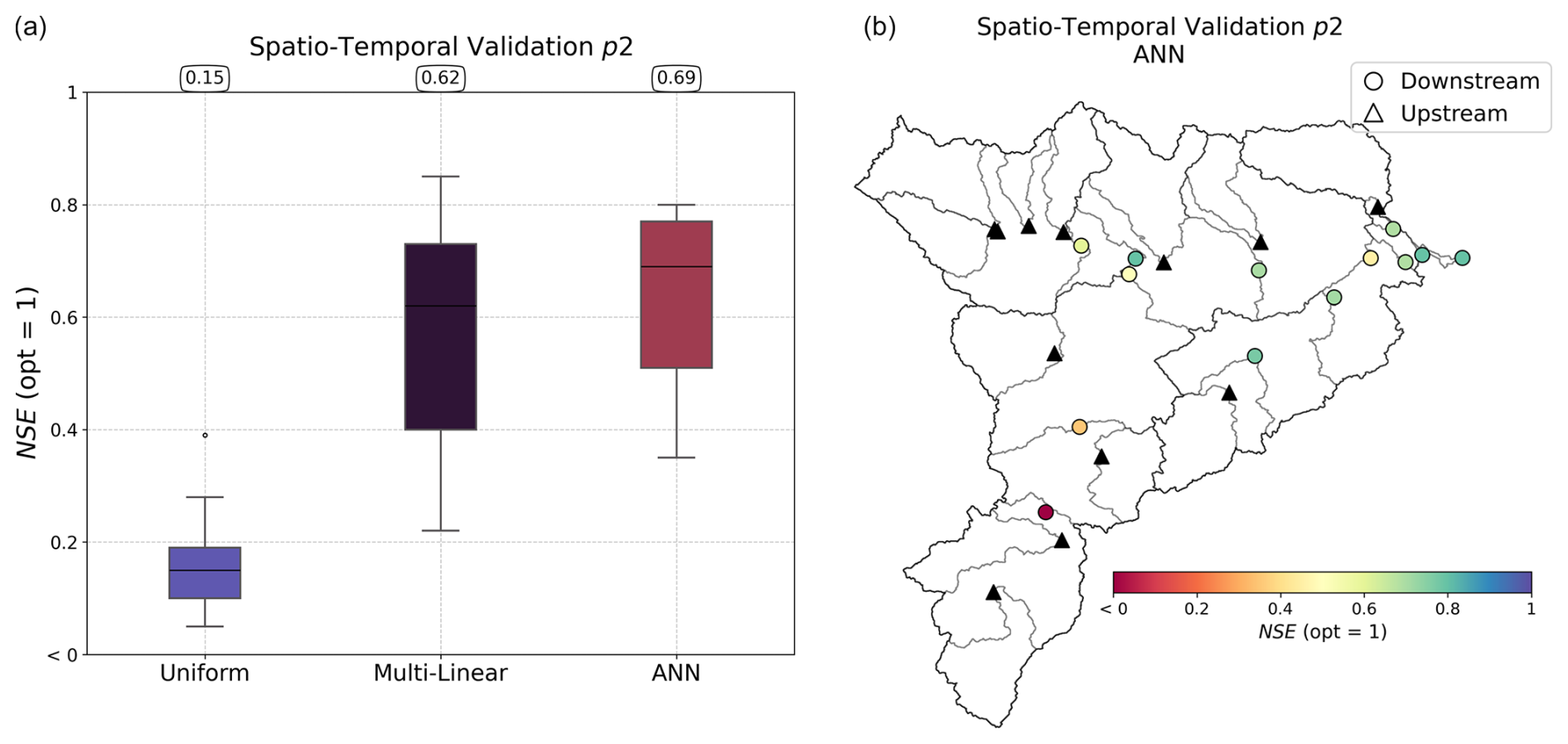
Figure 13 Performance in spatiotemporal validation over period p2 using calibration on upstream gauges (triangles). The boxplots in panel (a) represent the distribution of Nash–Sutcliffe efficiency (NSE) scores for the three calibration methods: uniform, multi-linear, and ANN. Median values are displayed at the top of each boxplot. The map in panel (b) illustrates the spatial distribution of the NSE values for the ANN mapping for the downstream validation catchments.

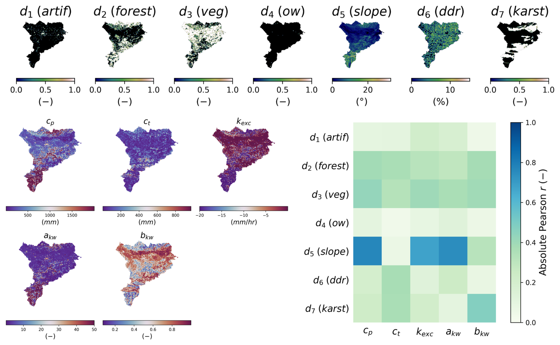
Figure 14 Analysis of input descriptors and output model parameters for the ANN descriptor-to-parameter mapping. Spatial distribution of physical descriptors (d₁–d₇) in the top panel, with details provided in Table 4. Spatial distribution of calibrated hydrological parameters (c_p, c_t, k_exc, a_kw, b_kw) in the lower-left panel and linear correlation between descriptors and parameters in the lower-right panel.

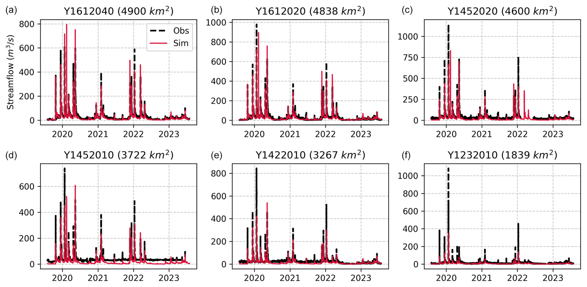
Figure 15 Observed and simulated streamflow of the six most downstream gauges of the Aude River for the ANN mapping. Each panel represents streamflow (m³ s⁻¹) for a specific gauge. The dashed black lines indicate observed values (Obs), while the solid red lines represent simulated values (Sim).

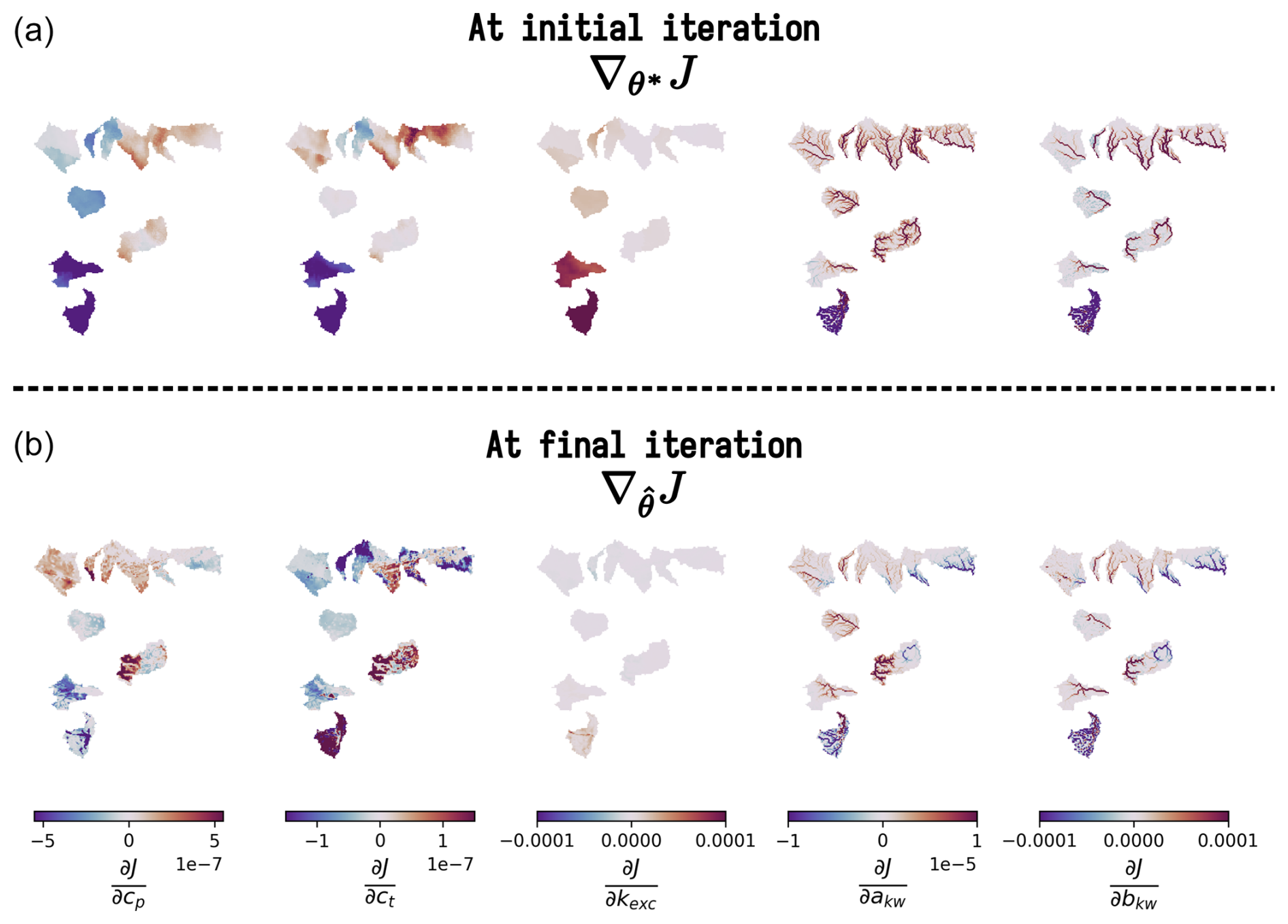
Figure 16 Spatially distributed gradients of the cost function J with respect to the model parameters at initial and final iterations for ANN mapping. The first row shows the gradients ${\mathrm{\nabla }}_{{\mathit{\theta }}^{\mathbf{*}}}J$ at the initial iteration, while the second row presents the gradients ${\mathrm{\nabla }}_{\widehat{\mathit{\theta }}}J$ at the final iteration after optimization. Each column corresponds to the partial derivative of J with respect to a specific parameter: c_p, c_t, k_exc, a_kw, and b_kw. These gradients are used in the optimization process of the control vector ρ using ${\mathrm{\nabla }}_{\mathit{\rho }}J={\mathrm{\nabla }}_{\mathit{\theta }}J.{\mathrm{\nabla }}_{\mathit{\rho }}\mathit{\theta }$ with $\mathit{\theta }=\mathcal{N}(.,\mathit{\rho })$, where 𝒩 is the multi-layer perceptron used.

4.4 France – Aude River: high-resolution regionalization

4.4.1 Numerical experiment settings

A set of 35 catchments (Fig. 7) over the Aude River in France (Addor et al., 2017) is evaluated in a regionalization context at a spatial resolution of 500 m and at an hourly time step using national databases (Table 4). This section is similar to the previous one, using the same regionalization method, but with differences in the gauges selected for calibration and validation and differences in the cost function. This section focuses on national data at a finer spatiotemporal scale, applying the method at the watershed level, which is more relevant for operational flood forecasting. The experimental design is as follows:

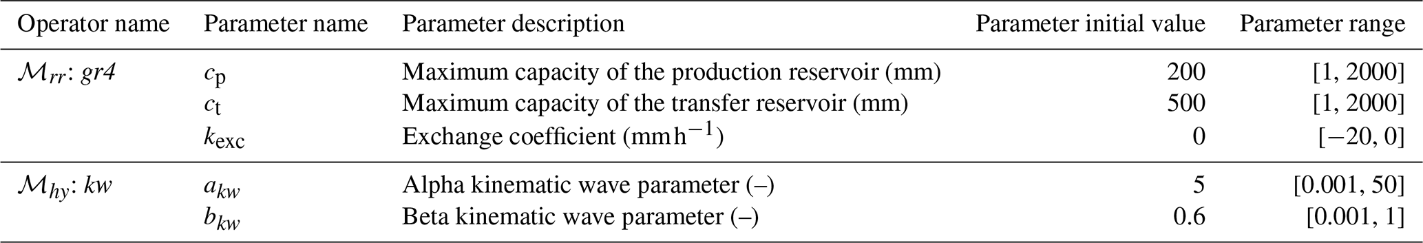
• One hydrological model is considered, identical to the gr4 model in Sect. 4.2 with the same routing module but without any snow modeling given the limited impact of snow in this Mediterranean basin (ℳ_snw: zero, ℳ_rr: gr4, ℳ_hy: kw). A description of the calibrated parameters is provided in Appendix C.

• A spatiotemporal validation procedure is set up by the following:

  • splitting the time window covered by hydrometric data into two complementary subsets over sub-periods of 4 years: p1 (from 1 August 2015 to 31 July 2019) and p2 (from 1 August 2019 to 31 July 2023), with p1 used as the calibration period and p2 as the validation period (for each period, 1 year is used as model “warm-up”)

  • splitting the catchment set into two groups, upstream and downstream, calibrating on the upstream group and validating on the downstream group.

• Three calibration mappings across the whole Aude River are tested:

  • Uniform. Spatially uniform parameters (gradient-free optimization) are used.

  • Multi-linear. Multiple linear regression is used as the transfer function from descriptors to spatialized parameters (gradient-based optimization).

  • ANN. A multi-layer perceptron composed of three hidden layers is used as the transfer function from descriptors to spatialized parameters (gradient-based optimization).

• A multi-gauge cost function is used based on the average NSE of the calibrated catchments ($J=\frac{\mathrm{1}}{N_G}{\sum }^{N_G}(\mathrm{1}-\text{NSE})$).

4.4.2 Results

The results of the regional mappings were validated on downstream gauges following Huynh et al. (2024b). The spatiotemporal validation performance, which assesses the model outside of the calibration gauges and period, is particularly challenging at such a high resolution and given the complex variabilities of physical factors and hydrological responses over this Mediterranean flash-flood-prone case. The results are shown in validation only, for brevity again, in Fig. 13. A uniform mapping yields a poor median NSE of 0.15, while descriptor-to-parameter mappings achieve 0.62 and 0.69 for multi-linear and ANN approaches respectively. Conceptual parameter maps obtained by learning from physical descriptors are shown in Fig. 14 for the ANN mapping only (with the best NSE result). The correlation matrix highlights significant correlations, especially between production capacity (c_p) and topographic slope (d₅) and between exchange parameter (k_exc) or routing parameter (a_kw) and topographic slope (d₅). For each parameter, a correlation is also found with vegetation cover rate (d₃) or forest cover rate (d₂). This illustrates the interpretability of our neural-network-based regionalization algorithm in the space of conceptual model parameters. Regarding computation times, the calibration with ANN mapping over period p1 took 31 h. This calibration involved 350 iterations, corresponding to 350 calls to the adjoint model, and was performed using 10 threads. For comparison, a single adjoint model run takes approximately 6 min, whereas a direct model run takes around 1 min and 30 s using the same number of threads. A key feature of smash is its ability to accurately and efficiently compute spatially distributed cost gradients, as shown in Fig. 16 in the conceptual parameter (θ) space for interpretability, in the case of a differentiable spatially distributed hydrological model that includes an NN-based regionalization mapping and a kinematic wave routing model (the partial differential equation numerical solver also being differentiated). Finally, simulated hydrographs are plotted for the six most downstream validation gauges in Fig. 15, with better reproduction for most downstream gauges in the present test configuration with the calibrated ANN regionalization (in agreements with results of Huynh et al., 2024b, over the whole French Mediterranean region).

These performances are very encouraging since they were obtained with a relatively simple regionalization setup in a complex flash-flood-prone area. Further research with smash will focus on improving the versatility of the hydrological model to better account for high rainfall intensities (e.g., Peredo et al., 2022) or groundwater/karstic effects, with classical or hybrid differential equations capable of learning from data at multiple scales, and to enrich regionalization algorithms with advanced cost functions and spatial relaxation/regularization strategies. These improvements are necessary to better extract information with the VDA algorithm from multiple discharge gauges and other data sources (descriptors, satellite moisture, temperature, etc.). Additionally, incorporating more realistic hydraulic routing embedded within the differentiable hydrologic model will also enable the integration of hydraulic information (water levels, flow videos, etc.), as introduced in Pujol et al. (2022).

5 Other smash features

In addition to the core differentiable spatialized hydrological solvers and regionalization learning algorithms illustrated above, smash enables performing the following:

• automatic hydrograph segmentation and flood detection over large samples (Huynh et al., 2023);

• parameter calibration using signature-based cost functions (Huynh et al., 2023) in addition to continuous metrics;

• parameter calibration using a spatial regularization term (Jay-Allemand et al., 2020);

• initial state estimation, including with regionalization mapping, even over short time windows, which is applicable to short-range VDA for operational forecasting;

• simulation of discharge ensembles from rainfall ensemble forecasting;

• Bayesian approach for parameter estimation and uncertainty quantification, with the consideration of structural model errors and observation errors.

6 Conclusions

The recently released smash framework represents an advancement in modular, regionalizable, and differentiable numerical modeling, as well as in hydrological data assimilation. This conclusion synthesizes the key principles, implementation features, performance indicators, and future prospects of smash, as presented in this article.

smash is built around three foundational principles: a modular operator chaining, enabling flexible representation of vertical and lateral hydrological processes; a regionalization mapping through hybrid approaches, combining conceptual models with descriptor-to-parameter neural networks; and a robust inverse algorithm that supports VDA.

The software leverages automatic differentiation to facilitate gradient-based calibration. Its seamless integration with Python via f90wrap ensures user-friendly access and flexibility, complemented by an automatic build system that simplifies deployment. Furthermore, smash supports parallel computing on CPUs, significantly accelerating computations for large-scale applications.

In terms of hydrological modeling, smash achieves interesting results. Using CAMELS datasets, a median KGE>0.8 is observed in local spatially distributed calibration for daily GR-like and VIC-like model structures at $\mathrm{d}x={\mathrm{1}}^{\prime }{\mathrm{30}}^{\prime \prime }$ (∼3 km). Additionally, regionalization learning across CONUS of conceptual parameters from physical descriptors yields KGE>0.6 in spatiotemporal validation. High-resolution hourly modeling at dx=500 m for Mediterranean flash-flood scenarios demonstrates NSE>0.6.

Planned enhancements to smash include the integration of additional differentiable hydrological, hydraulic, and land surface models; the expansion of hybrid physics–AI frameworks; and the refinement of data assimilation techniques. These advancements aim to further improve model accuracy, computational efficiency, and applicability in both research and operational settings.

Appendix A: CONUS – CAMELS: split-sample temporal cross-validation

Table A1 Summary of model operators and their associated parameters. For each operator, the parameter name, description, initial value, and allowable value range are provided.

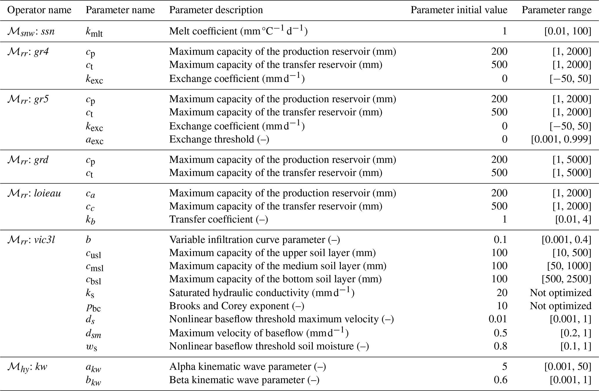
Table A2 Summary statistics of the calibrated parameters across the set of 482 catchments. For each parameter, the median, standard deviation, and coefficient of variation ($\mathit{\mu }/\mathit{\sigma }$) are reported for the two calibration configurations: spatially uniform (“Uniform”) and spatially distributed (“Distributed”). For the spatially distributed calibration, statistics were computed based on the spatial average of parameter values within each catchment.

Appendix B: CONUS – CAMELS: regionalization

Table B1 Summary of model operators and their associated parameters. For each operator, the parameter name, description, initial value, and allowable value range are provided.

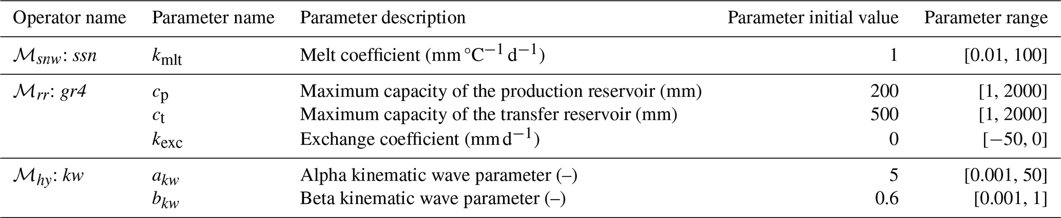
Table B2 Median KGE obtained in regionalization mapping calibration–validation over four groups of randomly selected basins.

Appendix C: France – Aude: high-resolution regionalization

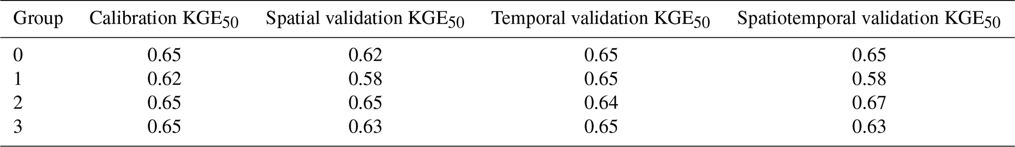
Table C1 Summary of model operators and their associated parameters. For each operator, the parameter name, description, initial value, and allowable value range are provided.

Appendix D: smash operators

This section describes the various operators available in smash with mathematical or numerical expressions, input data $\left[\mathit{I},\mathit{D}\right](x,t)$, tunable conceptual parameters θ(x,t), and simulated states and fluxes $\mathit{U}(x,t)=\left[Q,\mathit{h},\mathit{q}\right](x,t)$. These operators are written below for a given pixel x of the 2D spatial domain Ω and for a time t in the simulation window ]0,T].

D1 Snow operator ℳ_snw

• zero

  This snow operator simply means that there is no snow operator.

  $$m_{\mathit{\text{lt}}}(x,t)=\mathrm{0}$$

  Here m_lt is the melt flux.

• ssn

  This snow operator is a simple degree-day snow operator.

  Update the snow reservoir state h_s for $t^{*}\in \left]t-\mathrm{1},t\right[$:

  $$h_{\mathrm{s}}(x,t^{*})=h_{\mathrm{s}}(x,t-\mathrm{1})+S(x,t).$$

  Compute the melt flux m_lt:

  $$\begin{array}{ll}{\displaystyle }& {\displaystyle }{m}_{\mathit{\text{lt}}}(x,t)=\\ {\displaystyle }& {\displaystyle }\left\{\begin{array}{ll}\mathrm{0}& \text{if }{T}_e(x,t)\le \mathrm{0}\\ min\left(h_{\mathrm{s}}(x,t^{*}),k_{\text{mlt}}\left(x\right)\cdot T_e(x,t)\right)& \text{otherwise.}\end{array}\right.\end{array}$$

  Update the snow reservoir state h_s:

  $$h_{\mathrm{s}}(x,t)=h_{\mathrm{s}}(x,t^{*})-m_{\mathit{\text{lt}}}(x,t),$$

  with m_lt being the melt flux, S the snow, T_e the temperature, k_mlt the melt coefficient, and h_s the state of the snow reservoir.

D2 Hydrological operator ℳ_hy

• gr4

  This hydrological operator is derived from the GR4 model (Perrin et al., 2003).

  Interception

  Compute interception evapotranspiration e_i:

  $$\begin{array}{ll}{\displaystyle }& {\displaystyle }{e}_{\mathrm{i}}(x,t)=min\left(E\right(x,t),P(x,t)+m_{\mathit{\text{lt}}}(x,t)\\ {\displaystyle }& {\displaystyle }+\stackrel{\mathrm{̃}}{h_{\mathrm{i}}}(x,t-\mathrm{1})\cdot c_{\mathrm{i}}\left(x\right)).\end{array}$$

  Compute the neutralized precipitation p_n and evapotranspiration e_n:

  $$\begin{array}{ll}{\displaystyle }& {\displaystyle }{p}_{\mathrm{n}}(x,t)=max(\mathrm{0},P(x,t)+m_{\mathit{\text{lt}}}(x,t)\\ {\displaystyle }& {\displaystyle }-c_{\mathrm{i}}\left(x\right)(\mathrm{1}-\stackrel{\mathrm{̃}}{h_{\mathrm{i}}}(x,t-\mathrm{1}\left)\right)-e_{\mathrm{i}}(x,t))\\ {\displaystyle }& {\displaystyle }{e}_{\mathrm{n}}(x,t)=E(x,t)-e_{\mathrm{i}}(x,t).\end{array}$$

  Update the normalized interception reservoir state $\stackrel{\mathrm{̃}}{h_{\mathrm{i}}}$:

  $$\begin{array}{ll}{\displaystyle }\stackrel{\mathrm{̃}}{h_{\mathrm{i}}}(x,t)& {\displaystyle }=\stackrel{\mathrm{̃}}{h_{\mathrm{i}}}(x,t-\mathrm{1})\\ {\displaystyle }& {\displaystyle }+{\displaystyle \frac{P(x,t)+m_{\mathit{\text{lt}}}(x,t)+e_{\mathrm{i}}(x,t)-p_{\mathrm{n}}(x,t)}{c_{\mathrm{i}}\left(x\right)}}.\end{array}$$

  Production

  Compute the production infiltrating precipitation p_s and evapotranspiration e_s:

  $$\begin{array}{ll}{\displaystyle }{p}_{\mathrm{s}}(x,t)=& {\displaystyle }{c}_{\mathrm{p}}\left(x\right)\left(\mathrm{1}-\stackrel{\mathrm{̃}}{h_{\mathrm{p}}}(x,t-\mathrm{1}{)}^{\mathrm{2}}\right)\\ {\displaystyle }& {\displaystyle }\cdot {\displaystyle \frac{\tanh \left(\frac{p_{\mathrm{n}}(x,t)}{c_{\mathrm{p}}\left(x\right)}\right)}{\mathrm{1}+\stackrel{\mathrm{̃}}{h_{\mathrm{p}}}(x,t-\mathrm{1})\tanh \left(\frac{p_{\mathrm{n}}(x,t)}{c_{\mathrm{p}}\left(x\right)}\right)}}\\ {\displaystyle }{e}_{\mathrm{s}}(x,t)=& {\displaystyle }\stackrel{\mathrm{̃}}{h_{\mathrm{p}}}(x,t-\mathrm{1})\cdot c_{\mathrm{p}}\left(x\right)\cdot \left(\mathrm{2}-\stackrel{\mathrm{̃}}{h_{\mathrm{p}}}(x,t-\mathrm{1})\right)\\ {\displaystyle }& {\displaystyle }\cdot {\displaystyle \frac{\tanh \left(\frac{e_{\mathrm{n}}(x,t)}{c_{\mathrm{p}}\left(x\right)}\right)}{\mathrm{1}+\left(\mathrm{1}-\stackrel{\mathrm{̃}}{h_{\mathrm{p}}}(x,t-\mathrm{1})\right)\tanh \left(\frac{e_{\mathrm{n}}(x,t)}{c_{\mathrm{p}}\left(x\right)}\right)}}.\end{array}$$

  Update the normalized production reservoir state $\stackrel{\mathrm{̃}}{h_{\mathrm{p}}}$:

  $${\displaystyle }\stackrel{\mathrm{̃}}{h_{\mathrm{p}}}(x,t^{*})=\stackrel{\mathrm{̃}}{h_{\mathrm{p}}}(x,t-\mathrm{1})+{\displaystyle \frac{p_{\mathrm{s}}(x,t)-e_{\mathrm{s}}(x,t)}{c_{\mathrm{p}}\left(x\right)}}.$$

  Compute the production runoff p_r:

  $$\begin{array}{ll}{\displaystyle }& {\displaystyle }{p}_{\mathrm{r}}(x,t)=\\ {\displaystyle }& {\displaystyle }\left\{\begin{array}{l}\mathrm{0}\mathrm{\text{if }}{p}_{\mathrm{n}}(x,t)\le \mathrm{0}\\ p_{\mathrm{n}}(x,t)-\left(\stackrel{\mathrm{̃}}{h_{\mathrm{p}}}\right(x,t^{*})-\stackrel{\mathrm{̃}}{h_{\mathrm{p}}}(x,t-\mathrm{1}\left)\right)c_{\mathrm{p}}\left(x\right)\\ \mathrm{\text{otherwise}}.\end{array}\right.\end{array}$$

  Compute the production percolation p_erc:

  $$\begin{array}{ll}{\displaystyle }{p}_{\text{erc}}(x,t)=& {\displaystyle }\stackrel{\mathrm{̃}}{h_{\mathrm{p}}}(x,t^{*})\cdot c_{\mathrm{p}}\left(x\right)\\ {\displaystyle }& {\displaystyle }\cdot \left(\mathrm{1}-{\left(\mathrm{1}+{\left({\displaystyle \frac{\mathrm{4}}{\mathrm{9}}}\stackrel{\mathrm{̃}}{h_{\mathrm{p}}}(x,t^{*})\right)}^{\mathrm{4}}\right)}^{-\mathrm{1}/\mathrm{4}}\right).\end{array}$$

  Update the normalized production reservoir state $\stackrel{\mathrm{̃}}{h_{\mathrm{p}}}$:

  $${\displaystyle }\stackrel{\mathrm{̃}}{h_{\mathrm{p}}}(x,t)=\stackrel{\mathrm{̃}}{h_{\mathrm{p}}}(x,t^{*})-{\displaystyle \frac{p_{\text{erc}}(x,t)}{c_{\mathrm{p}}\left(x\right)}}.$$

  Exchange

  Compute the exchange flux l_exc:

  $${\displaystyle }{l}_{\text{exc}}(x,t)=k_{\text{exc}}\left(x\right)\cdot \stackrel{\mathrm{̃}}{h_{\mathrm{t}}}(x,t-\mathrm{1}{)}^{\mathrm{7}/\mathrm{2}}.$$

  Transfer

  Split the production runoff p_r into two branches (transfer and direct), p_rr and p_rd:

  $$\begin{array}{ll}{\displaystyle }& {\displaystyle }{p}_{\mathit{\text{rr}}}(x,t)=\mathrm{0.9}\left(p_{\mathrm{r}}(x,t)+p_{\text{erc}}(x,t)\right)+l_{\text{exc}}(x,t)\\ {\displaystyle }& {\displaystyle }{p}_{\mathit{\text{rd}}}(x,t)=\mathrm{0.1}\left(p_{\mathrm{r}}(x,t)+p_{\text{erc}}(x,t)\right).\end{array}$$

  Update the normalized transfer reservoir state $\stackrel{\mathrm{̃}}{h_{\mathrm{t}}}$:

  $${\displaystyle }\stackrel{\mathrm{̃}}{h_{\mathrm{t}}}(x,t^{*})=max\left(\mathrm{0},\stackrel{\mathrm{̃}}{h_{\mathrm{t}}}(x,t-\mathrm{1})+{\displaystyle \frac{p_{\mathit{\text{rr}}}(x,t)}{c_{\mathrm{t}}\left(x\right)}}\right).$$

  Compute the transfer branch elemental discharge q_r:

  $$\begin{array}{ll}{\displaystyle }{q}_r(x,t)=& {\displaystyle }\stackrel{\mathrm{̃}}{h_{\mathrm{t}}}(x,t^{*})\cdot c_{\mathrm{t}}\left(x\right)\\ {\displaystyle }& {\displaystyle }-{\left({\left(\stackrel{\mathrm{̃}}{h_{\mathrm{t}}}(x,t^{*})\cdot c_{\mathrm{t}}\left(x\right)\right)}^{-\mathrm{4}}+c_{\mathrm{t}}(x{)}^{-\mathrm{4}}\right)}^{-\mathrm{1}/\mathrm{4}}.\end{array}$$

  Update the normalized transfer reservoir state $\stackrel{\mathrm{̃}}{h_{\mathrm{t}}}$:

  $${\displaystyle }\stackrel{\mathrm{̃}}{h_{\mathrm{t}}}(x,t)=\stackrel{\mathrm{̃}}{h_{\mathrm{t}}}(x,t^{*})-{\displaystyle \frac{q_r(x,t)}{c_{\mathrm{t}}\left(x\right)}}.$$

  Compute the direct branch elemental discharge q_d:

  $${\displaystyle }{q}_d(x,t)=max\left(\mathrm{0},p_{\mathit{\text{rd}}}(x,t)+l_{\text{exc}}(x,t)\right).$$

  Compute the elemental discharge q_t:

  $${\displaystyle }{q}_t(x,t)=q_r(x,t)+q_d(x,t),$$

  with q_t being the elemental discharge, P the precipitation, E the potential evapotranspiration, m_lt the melt flux from the snow operator, c_i the maximum capacity of the interception reservoir, c_p the maximum capacity of the production reservoir, c_t the maximum capacity of the transfer reservoir, k_exc the exchange coefficient, $\stackrel{\mathrm{̃}}{h_{\mathrm{i}}}$ the state of the normalized interception reservoir, $\stackrel{\mathrm{̃}}{h_{\mathrm{p}}}$ the state of the normalized production reservoir, and $\stackrel{\mathrm{̃}}{h_{\mathrm{t}}}$ the state of the normalized transfer reservoir.

• gr5

  This hydrological operator is derived from the GR4 model (Le Moine, 2008). It consists of a GR4-like model structure (see above) with a modified exchange flux with two parameters to account for seasonal variations.

  Interception

  Same as gr4 Interception

  Production

  Same as gr4 Production

  Exchange

  Compute the exchange flux l_exc:

  $${\displaystyle }{l}_{\text{exc}}(x,t)=k_{\text{exc}}\left(x\right)\cdot \stackrel{\mathrm{̃}}{h_{\mathrm{t}}}(x,t-\mathrm{1}{)}^{\mathrm{7}/\mathrm{2}}.$$

  Transfer

  Same as gr4 Transfer, with q_t being the elemental discharge, P the precipitation, E the potential evapotranspiration, m_lt the melt flux from the snow operator, c_i the maximum capacity of the interception reservoir, c_p the maximum capacity of the production reservoir, c_t the maximum capacity of the transfer reservoir, k_exc the exchange coefficient, a_exc the exchange threshold, $\stackrel{\mathrm{̃}}{h_{\mathrm{i}}}$ the state of the normalized interception reservoir, $\stackrel{\mathrm{̃}}{h_{\mathrm{p}}}$ the state of the normalized production reservoir, and $\stackrel{\mathrm{̃}}{h_{\mathrm{t}}}$ the state of the normalized transfer reservoir.

• grd

  This hydrological operator is derived from the GR models and is a simplified structure used in Jay-Allemand et al. (2020).

  Interception

  Compute the interception evapotranspiration e_i:

  $${\displaystyle }{e}_{\mathrm{i}}(x,t)=min\left(E(x,t),P(x,t)+m_{\mathit{\text{lt}}}(x,t)\right).$$

  Compute the neutralized precipitation p_n and evapotranspiration e_n:

  $$\begin{array}{ll}{\displaystyle }& {\displaystyle }{p}_{\mathrm{n}}(x,t)=max\left(\mathrm{0},P(x,t)+m_{\mathit{\text{lt}}}(x,t)-e_{\mathrm{i}}(x,t)\right)\\ {\displaystyle }& {\displaystyle }{e}_{\mathrm{n}}(x,t)=E(x,t)-e_{\mathrm{i}}(x,t).\end{array}$$

  Production

  Same as gr4 Production

  Transfer

  Update the normalized transfer reservoir state $\stackrel{\mathrm{̃}}{h_{\mathrm{t}}}$:

  $${\displaystyle }\stackrel{\mathrm{̃}}{h_{\mathrm{t}}}(x,t^{*})=max\left(\mathrm{0},\stackrel{\mathrm{̃}}{h_{\mathrm{t}}}(x,t-\mathrm{1})+{\displaystyle \frac{p_{\mathrm{r}}(x,t)}{c_{\mathrm{t}}\left(x\right)}}\right).$$

  Compute the transfer branch elemental discharge q_r:

  $$\begin{array}{ll}{\displaystyle }{q}_r(x,t)& {\displaystyle }=\stackrel{\mathrm{̃}}{h_{\mathrm{t}}}(x,t^{*})\cdot c_{\mathrm{t}}\left(x\right)\\ {\displaystyle }& {\displaystyle }-{\left({\left(\stackrel{\mathrm{̃}}{h_{\mathrm{t}}}(x,t^{*})\cdot c_{\mathrm{t}}\left(x\right)\right)}^{-\mathrm{4}}+c_{\mathrm{t}}(x{)}^{-\mathrm{4}}\right)}^{-\mathrm{1}/\mathrm{4}}.\end{array}$$

  Update the normalized transfer reservoir state $\stackrel{\mathrm{̃}}{h_{\mathrm{t}}}$:

  $${\displaystyle }\stackrel{\mathrm{̃}}{h_{\mathrm{t}}}(x,t)=\stackrel{\mathrm{̃}}{h_{\mathrm{t}}}(x,t^{*})-{\displaystyle \frac{q_r(x,t)}{c_{\mathrm{t}}\left(x\right)}}.$$

  Compute the elemental discharge q_t:

  $${\displaystyle }{q}_t(x,t)=q_r(x,t),$$

  with q_t being the elemental discharge, P the precipitation, E the potential evapotranspiration, m_lt the melt flux from the snow operator, c_p the maximum capacity of the production reservoir, c_t the maximum capacity of the transfer reservoir, $\stackrel{\mathrm{̃}}{h_{\mathrm{p}}}$ the state of the normalized production reservoir, and $\stackrel{\mathrm{̃}}{h_{\mathrm{t}}}$ the state of the normalized transfer reservoir.

• loieau

  This hydrological operator is derived from the GR model (Folton and Arnaud, 2020).

  Interception

  Same as gr4 Interception

  Production

  Same as gr4 Production

  Transfer

  Split the production runoff p_r into two branches (transfer and direct), p_rr and p_rd:

  $$\begin{array}{ll}{\displaystyle }& {\displaystyle }{p}_{\mathit{\text{rr}}}(x,t)=\mathrm{0.9}\left(p_{\mathrm{r}}(x,t)+p_{\text{erc}}(x,t)\right)\\ {\displaystyle }& {\displaystyle }{p}_{\mathit{\text{rd}}}(x,t)=\mathrm{0.1}\left(p_{\mathrm{r}}(x,t)+p_{\text{erc}}(x,t)\right).\end{array}$$

  Update the normalized transfer reservoir state $\stackrel{\mathrm{̃}}{h_c}$:

  $${\displaystyle }\stackrel{\mathrm{̃}}{h_c}(x,t^{*})=max\left(\mathrm{0},\stackrel{\mathrm{̃}}{h_c}(x,t-\mathrm{1})+{\displaystyle \frac{p_{\mathit{\text{rr}}}(x,t)}{c_c\left(x\right)}}\right).$$

  Compute the transfer branch elemental discharge q_r:

  $$\begin{array}{ll}{\displaystyle }{q}_r(x,t)& {\displaystyle }=\stackrel{\mathrm{̃}}{h_c}(x,t^{*})\cdot c_c\left(x\right)\\ {\displaystyle }& {\displaystyle }-{\left({\left(\stackrel{\mathrm{̃}}{h_c}(x,t^{*})\cdot c_c\left(x\right)\right)}^{-\mathrm{3}}+c_c(x{)}^{-\mathrm{3}}\right)}^{-\mathrm{1}/\mathrm{3}}.\end{array}$$

  Update the normalized transfer reservoir state $\stackrel{\mathrm{̃}}{h_c}$:

  $${\displaystyle }\stackrel{\mathrm{̃}}{h_c}(x,t)=\stackrel{\mathrm{̃}}{h_c}(x,t^{*})-{\displaystyle \frac{q_r(x,t)}{c_c\left(x\right)}}.$$

  Compute the direct branch elemental discharge q_d:

  $${\displaystyle }{q}_d(x,t)=max\left(\mathrm{0},p_{\mathit{\text{rd}}}(x,t)\right).$$

  Compute the elemental discharge q_t:

  $${\displaystyle }{q}_t(x,t)=k_b\left(x\right)\cdot \left(q_r(x,t)+q_d(x,t)\right),$$

  with q_t being the elemental discharge, P the precipitation, E the potential evapotranspiration, m_lt the melt flux from the snow operator, c_a the maximum capacity of the production reservoir, c_c the maximum capacity of the transfer reservoir, k_b the transfer coefficient, $\stackrel{\mathrm{̃}}{h_a}$ the state of the normalized production reservoir, and $\stackrel{\mathrm{̃}}{h_c}$ the state of the normalized transfer reservoir.

• vic3l

  This hydrological operator is derived from the VIC model (Liang et al., 1994).

  Canopy layer interception

  Compute the canopy layer interception evapotranspiration e_c:

  $$\begin{array}{ll}{\displaystyle }{e}_c(x,t)=& {\displaystyle }min\left(E\right(x,t\left)\stackrel{\mathrm{̃}}{h_{\text{cl}}}\right(x,t-\mathrm{1}{)}^{\mathrm{2}/\mathrm{3}},\\ {\displaystyle }& {\displaystyle }P(x,t)+m_{\mathit{\text{lt}}}(x,t)+\stackrel{\mathrm{̃}}{h_{\text{cl}}}(x,t-\mathrm{1})).\end{array}$$

  Compute the neutralized precipitation p_n and evapotranspiration e_n:

  $$\begin{array}{ll}{\displaystyle }& {\displaystyle }{p}_{\mathrm{n}}(x,t)=max(\mathrm{0},P(x,t)+m_{\mathit{\text{lt}}}(x,t)\\ {\displaystyle }& {\displaystyle }-(\mathrm{1}-\stackrel{\mathrm{̃}}{h_{\text{cl}}}(x,t-\mathrm{1}\left)\right)-e_c(x,t))\\ {\displaystyle }& {\displaystyle }{e}_{\mathrm{n}}(x,t)=E(x,t)-e_c(x,t).\end{array}$$

  Update the normalized canopy layer interception state $\stackrel{\mathrm{̃}}{h_{\text{cl}}}$:

  $$\begin{array}{ll}{\displaystyle }\stackrel{\mathrm{̃}}{h_{\text{cl}}}(x,t)=& {\displaystyle }\stackrel{\mathrm{̃}}{h_{\text{cl}}}(x,t-\mathrm{1})+P(x,t)\\ {\displaystyle }& {\displaystyle }-e_c(x,t)-p_{\mathrm{n}}(x,t).\end{array}$$

  Upper soil layer evapotranspiration

  Compute the maximum infiltration i_m and the corresponding soil saturation infiltration i₀:

  $$\begin{array}{ll}{\displaystyle }& {\displaystyle }{i}_{\mathrm{m}}(x,t)=(\mathrm{1}+b(x\left)\right)c_{\text{usl}}\left(x\right)\\ {\displaystyle }& {\displaystyle }{i}_{\mathrm{0}}(x,t)=i_{\mathrm{m}}(x,t)\\ {\displaystyle }& {\displaystyle }\cdot (\mathrm{1}-(\mathrm{1}-\stackrel{\mathrm{̃}}{h_{\text{usl}}}(x,t-\mathrm{1}){)}^{\mathrm{1}/(\mathrm{1}-b(x\left)\right)}).\end{array}$$

  Compute the upper soil layer evapotranspiration e_s:

  $${\displaystyle }{e}_{\mathrm{s}}(x,t)=\left\{\begin{array}{ll}{e}_{\mathrm{n}}(x,t)& \text{if }{i}_{\mathrm{0}}(x,t)\ge i_m(x,t)\\ \mathit{\beta }(x,t)e_{\mathrm{n}}(x,t)& \text{otherwise},\end{array}\right.$$

  with β being the ARNO evapotranspiration beta function (Todini, 1996).

  Update the normalized upper soil layer reservoir state $\stackrel{\mathrm{̃}}{h_{\text{usl}}}$:

  $${\displaystyle }\stackrel{\mathrm{̃}}{h_{\text{usl}}}(x,t)=\stackrel{\mathrm{̃}}{h_{\text{usl}}}(x,t-\mathrm{1})-{\displaystyle \frac{e_{\mathrm{s}}(x,t)}{c_{\text{usl}}\left(x\right)}}.$$

  Infiltration

  Compute the maximum capacity c_umsl, soil moisture w_umsl, and relative state h_umsl of the first two layers:

  $$\begin{array}{ll}{\displaystyle }& {\displaystyle }{c}_{\text{umsl}}\left(x\right)=c_{\text{usl}}\left(x\right)+c_{\text{msl}}\left(x\right)\\ {\displaystyle }& {\displaystyle }{w}_{\text{umsl}}(x,t-\mathrm{1})=\stackrel{\mathrm{̃}}{h_{\text{usl}}}(x,t-\mathrm{1})c_{\text{usl}}\left(x\right)\\ {\displaystyle }& {\displaystyle }+\stackrel{\mathrm{̃}}{h_{\text{msl}}}(x,t-\mathrm{1})c_{\text{msl}}\left(x\right)\\ {\displaystyle }& {\displaystyle }{h}_{\text{umsl}}(x,t-\mathrm{1})={\displaystyle \frac{w_{\text{umsl}}(x,t-\mathrm{1})}{c_{\text{umsl}}\left(x\right)}}.\end{array}$$

  Compute maximum i_m and infiltration i₀:

  $$\begin{array}{ll}{\displaystyle }{i}_{\mathrm{m}}(x,t)=& {\displaystyle }(\mathrm{1}+b(x\left)\right)c_{\text{umsl}}\left(x\right)\\ {\displaystyle }{i}_{\mathrm{0}}(x,t)=& {\displaystyle }{i}_{\mathrm{m}}(x,t)\\ {\displaystyle }& {\displaystyle }\cdot (\mathrm{1}-(\mathrm{1}-h_{\text{umsl}}(x,t-\mathrm{1}){)}^{\mathrm{1}/(\mathrm{1}-b(x\left)\right)}).\end{array}$$

  Compute infiltration i:

  $${\displaystyle }i(x,t)=\left\{\begin{array}{l}{c}_{\text{umsl}}\left(x\right)-w_{\text{umsl}}(x,t-\mathrm{1})\\ \mathrm{\text{if }}{i}_{\mathrm{0}}(x,t)+p_{\mathrm{n}}(x,t)>i_m(x,t)\\ \begin{array}{l}{c}_{\text{umsl}}\left(x\right)-w_{\text{umsl}}(x,t-\mathrm{1})\\ -c_{\text{umsl}}\left(x\right){\left(\mathrm{1}-\frac{i_{\mathrm{0}}(x,t)+p_{\mathrm{n}}(x,t)}{i_m(x,t)}\right)}^{b\left(x\right)+\mathrm{1}}\end{array}\\ \mathrm{\text{otherwise}}.\end{array}\right.$$

  Distribute infiltration between the upper two layers:

  $$\begin{array}{ll}{\displaystyle }{i}_{\text{usl}}(x,t)=min(& {\displaystyle }(\mathrm{1}-\stackrel{\mathrm{̃}}{h_{\text{usl}}}(x,t-\mathrm{1}\left)\right)c_{\text{usl}}\left(x\right),\\ {\displaystyle }& {\displaystyle }i(x,t))\\ {\displaystyle }{i}_{\text{msl}}(x,t)=min(& {\displaystyle }(\mathrm{1}-\stackrel{\mathrm{̃}}{h_{\text{msl}}}(x,t-\mathrm{1}\left)\right)c_{\text{msl}}\left(x\right),\\ {\displaystyle }& {\displaystyle }i(x,t)-i_{\text{usl}}(x,t)).\end{array}$$

  Update the reservoir states:

  $$\begin{array}{ll}{\displaystyle }\stackrel{\mathrm{̃}}{h_{\text{usl}}}(x,t)& {\displaystyle }=\stackrel{\mathrm{̃}}{h_{\text{usl}}}(x,t-\mathrm{1})+i_{\text{usl}}(x,t)\\ {\displaystyle }\stackrel{\mathrm{̃}}{h_{\text{msl}}}(x,t)& {\displaystyle }=\stackrel{\mathrm{̃}}{h_{\text{msl}}}(x,t-\mathrm{1})+i_{\text{msl}}(x,t).\end{array}$$

  Compute runoff:

  $${\displaystyle }{q}_r(x,t)=p_{\mathrm{n}}(x,t)-\left(i_{\text{usl}}\right(x,t)+i_{\text{msl}}(x,t\left)\right).$$

  Drainage

  Compute the soil moisture in the first two layers:

  $$\begin{array}{ll}{\displaystyle }{w}_{\text{usl}}(x,t-\mathrm{1})& {\displaystyle }=\stackrel{\mathrm{̃}}{h_{\text{usl}}}(x,t-\mathrm{1})c_{\text{usl}}\left(x\right)\\ {\displaystyle }{w}_{\text{msl}}(x,t-\mathrm{1})& {\displaystyle }=\stackrel{\mathrm{̃}}{h_{\text{msl}}}(x,t-\mathrm{1})c_{\text{msl}}\left(x\right).\end{array}$$

  Compute the initial drainage flux:

  $${\displaystyle }{d}_{\text{umsl}}(x,t^{*})=k_s\left(x\right)\cdot \stackrel{\mathrm{̃}}{h_{\text{usl}}}(x,t-\mathrm{1}{)}^{p_{\text{bc}}}.$$

  Update the drainage flux:

  $$\begin{array}{ll}{\displaystyle }& {\displaystyle }{d}_{\text{umsl}}(x,t)=min\left(d_{\text{umsl}}\right(x,t^{*}),\\ {\displaystyle }& {\displaystyle }min\left(w_{\text{usl}}\right(x,t-\mathrm{1}),c_{\text{msl}}(x)-w_{\text{msl}}(x,t-\mathrm{1}\left)\right)).\end{array}$$

  Update normalized reservoir states:

  $$\begin{array}{ll}{\displaystyle }\stackrel{\mathrm{̃}}{h_{\text{usl}}}(x,t)& {\displaystyle }=\stackrel{\mathrm{̃}}{h_{\text{usl}}}(x,t-\mathrm{1})-{\displaystyle \frac{d_{\text{umsl}}(x,t)}{c_{\text{usl}}\left(x\right)}}\\ {\displaystyle }\stackrel{\mathrm{̃}}{h_{\text{msl}}}(x,t)& {\displaystyle }=\stackrel{\mathrm{̃}}{h_{\text{msl}}}(x,t-\mathrm{1})+{\displaystyle \frac{d_{\text{umsl}}(x,t)}{c_{\text{msl}}\left(x\right)}}.\end{array}$$

  The same approach is performed for drainage between medium and bottom soil layers. For brevity, we skip the first steps and directly give the update equations.

  Update the normalized medium and bottom reservoir states:

  $$\begin{array}{ll}{\displaystyle }\stackrel{\mathrm{̃}}{h_{\text{msl}}}(x,t)& {\displaystyle }=\stackrel{\mathrm{̃}}{h_{\text{msl}}}(x,t-\mathrm{1})-{\displaystyle \frac{d_{\mathit{\text{mbsl}}}(x,t)}{c_{\text{msl}}\left(x\right)}}\\ {\displaystyle }\stackrel{\mathrm{̃}}{h_{\text{bsl}}}(x,t)& {\displaystyle }=\stackrel{\mathrm{̃}}{h_{\text{bsl}}}(x,t-\mathrm{1})+{\displaystyle \frac{d_{\mathit{\text{mbsl}}}(x,t)}{c_{\text{bsl}}\left(x\right)}}.\end{array}$$

  Baseflow

  Compute baseflow q_b:

  $$\begin{array}{ll}{\displaystyle }& {\displaystyle }{q}_b(x,t)=\\ {\displaystyle }& {\displaystyle }\left\{\begin{array}{ll}\frac{d_{\mathit{\text{sm}}}\left(x\right)d_s\left(x\right)}{w_{\mathrm{s}}\left(x\right)}\stackrel{\mathrm{̃}}{h_{\text{bsl}}}(x,t-\mathrm{1})& \\ \mathrm{\text{if }}\stackrel{\mathrm{̃}}{h_{\text{bsl}}}(x,t-\mathrm{1})\le w_{\mathrm{s}}\left(x\right)& \\ \begin{array}{l}\frac{d_{\mathit{\text{sm}}}\left(x\right)d_s\left(x\right)}{w_{\mathrm{s}}\left(x\right)}\stackrel{\mathrm{̃}}{h_{\text{bsl}}}(x,t-\mathrm{1})\\ +d_{\mathit{\text{sm}}}\left(x\right)\left(\mathrm{1}-\frac{d_s\left(x\right)}{w_{\mathrm{s}}\left(x\right)}\right){\left(\frac{\stackrel{\mathrm{̃}}{h_{\text{bsl}}}(x,t-\mathrm{1})-w_{\mathrm{s}}\left(x\right)}{\mathrm{1}-w_{\mathrm{s}}\left(x\right)}\right)}^{\mathrm{2}}\end{array}& \\ \mathrm{\text{otherwise}}.\end{array}\right.\end{array}$$

  Update the normalized bottom soil layer reservoir:

  $${\displaystyle }\stackrel{\mathrm{̃}}{h_{\text{bsl}}}(x,t)=\stackrel{\mathrm{̃}}{h_{\text{bsl}}}(x,t-\mathrm{1})-{\displaystyle \frac{q_b(x,t)}{c_{\text{bsl}}\left(x\right)}},$$

  with q_t being the elemental discharge, P the precipitation, E the potential evapotranspiration, m_lt the melt flux from the snow operator, b the variable infiltration curve parameter, c_usl the maximum capacity of the upper soil layer, c_msl the maximum capacity of the medium soil layer, c_bsl the maximum capacity of the bottom soil layer, k_s the saturated hydraulic conductivity, p_bc the Brooks and Corey exponent, d_sm the maximum velocity of baseflow, d_s the nonlinear baseflow threshold maximum velocity, w_s the nonlinear baseflow threshold soil moisture, $\stackrel{\mathrm{̃}}{h_{\text{cl}}}$ the state of the normalized canopy layer, $\stackrel{\mathrm{̃}}{h_{\text{usl}}}$ the state of the normalized upper soil layer, $\stackrel{\mathrm{̃}}{h_{\text{msl}}}$ the state of the normalized medium soil layer, and $\stackrel{\mathrm{̃}}{h_{\text{bsl}}}$ the state of the normalized bottom soil layer.

D3 Routing operator ℳ_rr

• lag0

  This routing operator is a simple aggregation of upstream discharge to downstream discharge following the drainage plan.

  Upstream discharge

  Compute the upstream discharge q_up:

  $${\displaystyle }{q}_{\text{up}}(x,t)=\left\{\begin{array}{ll}\mathrm{0}& \text{if }{\mathrm{\Omega }}_x=\mathrm{\varnothing }\\ \sum _{k\in {\mathrm{\Omega }}_x}Q(k,t)& \text{otherwise},\end{array}\right.$$

  where Ω_x is the set of upstream cells flowing into cell x.

  Surface discharge

  Compute the surface discharge Q:

  $${\displaystyle }Q(x,t)=q_{\text{up}}(x,t)+\mathit{\alpha }\left(x\right)q_t(x,t),$$

  where α(x) is a unit conversion factor from $\text{mm}\cdot \mathrm{\Delta }{t}^{-\mathrm{1}}$ to ${\mathrm{m}}^{\mathrm{3}}\cdot {\mathrm{s}}^{-\mathrm{1}}$ for a single cell.

  Q is the surface discharge, q_t is the elemental discharge, and Ω_x is a 2D spatial domain that corresponds to all upstream cells flowing into cell x, i.e., the whole upstream catchment. Note that Ω_x is a subset of Ω, Ω_x⊂Ω, and for the most upstream cells Ω_x=∅.

• lr

  This routing operator uses a linear reservoir to route upstream discharge to downstream discharge following the drainage plan.

  Upstream discharge

  Same as lag0 Upstream discharge

  Surface discharge

  Update the routing reservoir state h_lr:

  $${\displaystyle }{h}_{\mathit{\text{lr}}}(x,t^{*})=h_{\mathit{\text{lr}}}(x,t)+{\displaystyle \frac{\mathrm{1}}{\mathit{\beta }\left(x\right)}}{q}_{\text{up}}(x,t),$$

  where β(x) is a conversion factor from $\text{mm}\cdot \mathrm{\Delta }{t}^{-\mathrm{1}}$ to ${\mathrm{m}}^{\mathrm{3}}\cdot {\mathrm{s}}^{-\mathrm{1}}$ for the entire upstream domain Ω_x.

  Compute the routed discharge q_rt:

  $${\displaystyle }{q}_{\mathit{\text{rt}}}(x,t)=h_{\mathit{\text{lr}}}(x,t^{*})\left(\mathrm{1}-\exp \left({\displaystyle \frac{-\mathrm{\Delta }t}{\mathrm{60}\times l_{\mathit{\text{lr}}}}}\right)\right).$$

  Update the routing reservoir state h_lr:

  $${\displaystyle }{h}_{\mathit{\text{lr}}}(x,t)=h_{\mathit{\text{lr}}}(x,t^{*})-q_{\mathit{\text{rt}}}(x,t).$$

  Compute the surface discharge Q:

  $${\displaystyle }Q(x,t)=\mathit{\beta }\left(x\right)q_{\mathit{\text{rt}}}(x,t)+\mathit{\alpha }\left(x\right)q_t(x,t),$$

  where α(x) is a conversion factor from $\text{mm}\cdot \mathrm{\Delta }{t}^{-\mathrm{1}}$ to ${\mathrm{m}}^{\mathrm{3}}\cdot {\mathrm{s}}^{-\mathrm{1}}$ for a single cell.

• kw

  This routing operator is based on a conceptual 1D kinematic wave model that is numerically solved with a linearized implicit numerical scheme (Chow et al., 1998). This is applicable given the drainage plan 𝒟_Ω(x) that enables the routing problem to be reduced to 1D.

  The kinematic wave model is a simplification of the 1D Saint-Venant hydraulic equations.

  First, the mass conservation equation is written as

  $$\begin{array}{}\text{(D1)}& {\displaystyle }{\displaystyle \frac{\partial A}{\partial t}}+{\displaystyle \frac{\partial Q}{\partial x}}=q,\end{array}$$

  where ${\partial }_{\square }$ denotes partial differentiation with respect to time or space, A is the cross-sectional flow area, Q is the discharge, and q represents lateral inflows.

  The momentum equation is simplified by assuming that the water surface slope equals the bed slope; i.e., the flow is locally uniform and gradually varied:

  $$\begin{array}{}\text{(D2)}& {\displaystyle }{\displaystyle }{S}_{\mathrm{0}}=S_f,\end{array}$$

  where S₀ is the bed slope, and S_f is the friction slope. This implies that the energy grade line is parallel to the channel bottom.

  This simplification leads to an empirical relation between discharge and flow area or depth, as described by Chow et al. (1998):

  $$\begin{array}{}\text{(D3)}& {\displaystyle }{\displaystyle }A=a_{\mathit{\text{kw}}}{Q}^{b_{\mathit{\text{kw}}}},\end{array}$$

  where a_kw and b_kw are two empirical constants that can also be related to the Manning friction law.

  Injecting the parameterization from Eq. (D3) into the mass conservation equation (Eq. D1) yields the following one-equation form of the kinematic wave model (Chow et al., 1998):

  $$\begin{array}{}\text{(D4)}& {\displaystyle }{\displaystyle \frac{\partial Q}{\partial x}}+a_{\mathit{\text{kw}}}{b}_{\mathit{\text{kw}}}{Q}^{b_{\mathit{\text{kw}}}-\mathrm{1}}{\displaystyle \frac{\partial Q}{\partial t}}=q.\end{array}$$

  For the sake of clarity, the following variables are renamed for this section and the finite-difference numerical scheme.

Table D1 Renamed variables.

Upstream discharge

Same as lag0 Upstream discharge with q_up denoted $Q_{i-\mathrm{1}}^j$.

Surface discharge

Compute the intermediate variables d₁ and d₂:

$$\begin{array}{ll}{\displaystyle }{d}_{\mathrm{1}}& {\displaystyle }={\displaystyle \frac{\mathrm{\Delta }t}{\mathrm{\Delta }x}},\\ {\displaystyle }{d}_{\mathrm{2}}& {\displaystyle }=a_{\mathit{\text{kw}}}{b}_{\mathit{\text{kw}}}{\left({\displaystyle \frac{Q_i^{j-\mathrm{1}}+Q_{i-\mathrm{1}}^j}{\mathrm{2}}}\right)}^{b_{\mathit{\text{kw}}}-\mathrm{1}}.\end{array}$$

Compute the intermediate variables n₁, n₂, and n₃:

$$\begin{array}{ll}{\displaystyle }{n}_{\mathrm{1}}& {\displaystyle }=d_{\mathrm{1}}{Q}_{i-\mathrm{1}}^j,\\ {\displaystyle }{n}_{\mathrm{2}}& {\displaystyle }=d_{\mathrm{2}}{Q}_i^{j-\mathrm{1}},\\ {\displaystyle }{n}_{\mathrm{3}}& {\displaystyle }=d_{\mathrm{1}}{\displaystyle \frac{q_i^{j-\mathrm{1}}+q_i^j}{\mathrm{2}}}.\end{array}$$

Compute the surface discharge $Q_i^j$:

$$Q_i^j=Q(x,t)={\displaystyle \frac{n_{\mathrm{1}}+n_{\mathrm{2}}+n_{\mathrm{3}}}{d_{\mathrm{1}}+d_{\mathrm{2}}}},$$

with Q being the surface discharge, q_t the elemental discharge, a_kw the alpha kinematic wave parameter, b_kw the beta kinematic wave parameter, and Ω_x a 2D spatial domain that corresponds to all upstream cells flowing into cell x. Note that Ω_x is a subset of Ω, Ω_x⊂Ω, and for the most upstream cells Ω_x=∅.

Appendix E: CPU information

Architecture:             x86_64
  CPU op-mode(s):         32 bit, 64 bit
  Address sizes:          48 bits physical, 48 bits virtual
  Byte order:             Little Endian
CPU(s):                   192
  On-line CPU(s) list:    0-191
Vendor ID:                AuthenticAMD
  Model name:             AMD EPYC 7643 48-Core Processor
    CPU family:           25
    Model:                1
    Thread(s) per core:   2
    Core(s) per socket:   48
    Socket(s):            2
    Stepping:             1
    Frequency boost:      enabled
    CPU max MHz:          2300.0000
    CPU min MHz:          1500.0000
    BogoMIPS:             4591.48
Virtualization features:
  Virtualization:         AMD-V
Caches (sum of all):
  L1d:                    3 MiB (96 instances)
  L1i:                    3 MiB (96 instances)
  L2:                     48 MiB (96 instances)
  L3:                     512 MiB (16 instances)
NUMA:
  NUMA node(s):           2
  NUMA node0 CPU(s):      0-47,96-143
  NUMA node1 CPU(s):      48-95,144-191