FastCTM (v1.0): Atmospheric chemical transport modelling with a principle-informed neural network for air quality simulations

Chemical-transport models (CTMs) are indispensable for air-quality assessment and policy development, yet their operational use is hampered by high computational cost. We present FastCTM, a physics-informed neural-network emulator that rapidly predicts hourly concentrations of ten key pollutant variables: major PM_2.5 species (SO${}_{\mathrm{4}}^{\mathrm{2}-}$, NO${}_{\mathrm{3}}^{-}$, NH${}_{\mathrm{4}}^{-}$, organic matter, elemental carbon, crustal material), coarse PM₁₀, SO₂, NO₂, CO, and O₃. FastCTM embeds five process-specific neural modules – primary emissions, horizontal transport, turbulent diffusion, chemical reactions and deposition within a unified framework. Given 1 h initial condition data, FastCTM can simulate future 24 h concentrations for ten air pollutants using corresponding meteorological fields and emissions as input. Trained on 2018–2022 WRF-CMAQ forecasts over China and evaluated on 2023 data, FastCTM reproduces CMAQ with mean RMSE (µg m⁻³) of 9.1, 11.9, 4.4, 4.0, 48.9, 10.9 and R² of 0.80, 0.81, 0.80, 0.83, 0.90, 0.70 for PM_2.5, PM₁₀, SO₂, NO₂, CO and O₃, respectively. Sensitivity tests confirm physically plausible responses to temperature, wind speed, boundary-layer height and precursor emissions. The modular architecture enables quantitative process analysis, offering CTM-like insight at GPU-accelerated speeds. In a nutshell, FastCTM provides a computationally efficient solution for air-quality simulations, sensitivity analysis, and process attribution with high accuracy and physical consistency.

1 Introduction

Effective air quality management requires accurate characterization of current and future pollution conditions to implement targeted emission control measures (Wang et al., 2010; Council, 2004). Driven by this demand, deterministic air quality numerical models have been developed to simulate the spatiotemporal variability and evolution of ambient air pollutants in the atmosphere (Hakami et al., 2003; Eder et al., 2006). In these models, such as the Community Multiscale Air Quality (CMAQ) model, atmospheric physical and chemical processes (e.g., emissions, chemical reactions, horizontal advection, and diffusion) are mathematically represented by partial differential equations. The air pollutant and species concentrations can then be calculated by solving these complex equations using numerical methods (Byun and Schere, 2006), which is often time-consuming (Leal et al., 2017) and requires substantial computational resources such as high-performance computing (Efstathiou et al., 2024).

Deep learning offers promising alternatives for developing rapid, data-driven CTMs by leveraging the capacity of neural networks to encode complex spatiotemporal patterns from large datasets (LeCun et al., 2015; He et al., 2016; Liao et al., 2020). These deep learning-based CTM models are expected to provide accurate simulations that are comparable to the current deterministic numerical CTMs while offering much higher computational efficiency and enhanced learning capabilities. However, progress has been hindered by challenges in designing neural architectures that simultaneously achieve high accuracy, interpretability, and long-term simulation stability and fidelity (Reichstein et al., 2019; Irrgang et al., 2021). In constructing deep learning-based CTM models, air quality modeling is often formulated as a sequence-to-sequence prediction problem (Shi et al., 2015; Zhang et al., 2024) to capture the spatiotemporal correlations among multiple variables. Consequently, previous studies have mainly focused on refining neural network's representation capabilities by proposing new neural-network structures to improve error back-propagation efficiencies and model encoding capabilities (Wang et al., 2018; Huang et al., 2021; Mao et al., 2021). For example, Xing et al. (2022) developed a deep learning-based module named deepCTM that mimics atmospheric photochemical modeling to simulate ozone concentrations. However, these deep learning-based CTMs are often structured as uninterpretable black-box models that generate simulations reflecting the cumulative effect of all physical and chemical processes. Such black-box models hinder error attribution, inspection of internal processes, and knowledge discovery (Reichstein et al., 2019).

Quantifying individual atmospheric processes enables a mechanistic interpretation of model predictions and identification of error sources (Liu et al., 2010). Motivated by this need, recent studies have developed models that learn specific atmospheric processes, such as chemical reactions and deposition, within CTM frameworks. Kelp et al. (2022) developed a neural network chemical solver for stable long-term global simulations of atmospheric chemistry, trained from the GEOS-Chem model. Xia et al. (2025) simulated 74 chemical species and 229 reactions following the SAPRC-99 mechanism using an artificial intelligence photochemistry (AIPC) scheme, achieving approximately 8-fold speed-up. Sturm and Wexler (2020) developed a mass- and energy-conserving framework for using machine learning to accelerate computations, demonstrating successful application in a photochemistry example. For the deposition process, Silva et al. (2019) proposed a deep learning parameterization for ozone dry deposition velocities that provided accurate predictions on independent new datasets, revealing the potential of neural networks to capture complex spatio-temporal latent processes. Liu et al. (2025) proposed a Neural Network Emulator, named ChemNNE, for rapid chemical concentration modelling, which achieved strong performance in both accuracy and efficiency. Although these successes, a gap remains in coupling these NN operators into a complete deep-learning CTM.

The main objective of our study is to develop and validate a principles-guided, neural network-based FastCTM, capable of simulating spatial-temporal fields of hourly concentrations of 10 criteria pollutants, including major species of PM_2.5 (SO${}_{\mathrm{4}}^{\mathrm{2}-}$, NO${}_{\mathrm{3}}^{-}$, NH${}_{\mathrm{4}}^{+}$, organic matters and other inorganic components, coarse part in PM₁₀, CO, NO₂, SO_2, and O₃. FastCTM models individual atmospheric process: transport, diffusion, deposition, chemical reactions, and emissions. FastCTM is capable of performing analysis of internal chemical and physical processes, offering benefits like high computational speed, efficient data assimilation, and rapid model updates.

2 Data and Methods

2.1 Parent Model Simulations and Datasets

In this study, the FastCTM model was designed to replicate the parent model CMAQ, trained by learning CMAQ's underlying physical and chemical processes among multiple air pollutants, including the complicated chemical reaction, transport, diffusion, and deposition. CMAQ has a process analysis (PA) tool to separate out and quantify the contributions of individual physical and chemical processes to the changes in the predicted concentrations of a pollutant, which provides the opportunity to conduct a sensitivity analysis by comparing process contributions between CMAQ and FastCTM.

Weather and air quality simulations from 2018 to 2023 were conducted using a WRF-CMAQ modeling system consisting of three major components: (1) the meteorology component, the Weather Research and Forecasting model, WRF v3.4.1 (Michalakes et al., 2005; Skamarock et al., 2008), which provides meteorological fields; provides meteorological fields, (2) the emission component, which supplies gridded estimates of hourly emission rates for primary pollutants matched to model species, and (3) the CTM component, CMAQ v5.0.2 (Byun and Schere, 2006), which solves the governing physical and chemical equations to obtain 3-D pollutant concentration fields. WRF-CMAQ simulations are not two-way coupled, so weather and chemistry do not influence each other. We used hourly average concentrations of dominant PM_2.5 components of sulfate (SO₄), nitrate (NO₃), ammonium (NH₄), organic carbon (OC), and other components (EC and soil, etc.), and CO, SO₂, NO_2, and O₃ in the surface layer. The 10 species were selected based on their direct relevance to regulatory standards (e.g., PM_2.5, PM₁₀, O₃, NO₂, SO₂, and CO) and their dominance in driving health and environmental impacts in urban and industrial regions.

Meteorological variables used in this study include relative humidity (RH), air temperature (T), wind components (U, V) at surface 10 m height, precipitation (RN), cloud fraction (CFRAC), and planetary boundary layer height (PBLH). Wind speed (WS) was calculated from U and V. The data covered the whole of China at a horizontal resolution of 12 km with 372 × 426 grid cells. The simulation data from 2018–2022 are used as the training dataset, while the remaining simulation data in 2023 is used for independent evaluation. The surface topographic data (HGT, Fig. S1 in the Supplement, obtained from https://lta.cr.usgs.gov/GTOPO30, last access: 28 July 2023) and land cover data (Zhang et al., 2021) of urban and tree fraction (LULC) are also used to reflect the effects of land surface conditions in this study.

The original primary emissions used in the aforementioned WRF-CMAQ modelling system are used as input to the FastCTM. The large amount of emission data is grouped according to the simulated 10 pollutant variables. Specifically, the primary PM_2.5 emissions of SO₄, NO₃, NH₄, OC, and other components, and gaseous emissions including sulfur oxide (SO₂), nitrogen oxides (NO_x, including HONO, NO, and NO₂), ammonia (NH₃), volatile organic species (VOCs, including isoprene (ISOP), terpene (TERP), and other species of VOC) are used in the FastCTM. Annual average emissions of NO_x, SO₂, and VOC are respectively depicted in Figs. S2–S4 in the Supplement.

2.2 FastCTM Model Formulations

2.2.1 FastCTM Model Framework

The deterministic CTM models simulate emissions, transport, deposition, diffusion, and chemical transformations of gases and particles in the troposphere through numerically solving the governing equations as follows,

$$\begin{array}{}\text{(1)}& {\displaystyle \frac{\partial C_i}{\partial t}}=-\mathrm{\nabla }\cdot \left(\mathit{u}{C}_i\right)+\mathrm{\nabla }\left(K\mathrm{\nabla }{C}_i\right)+R_i+E_i+D_i\end{array}$$

where C_i is the concentration of species i, u is the air fluid velocity, K is the eddy diffusivity tensor, R_i is the net rate of chemical generation of species i, E_i is the rate of direct addition of the species from primary emissions, and D_i is the deposition rate caused by both dry and wet depositions. A detailed description of CMAQ principles is available elsewhere (Byun and Schere, 2006; Appel et al., 2017). Inspired by numerical CTMs principles and equations, the guiding framework of FastCTM was also structured in a similar formulation to represent the dominant processes in order to simulate air pollutant spatiotemporal variations.

In the context of deep learning, hourly air quality simulation is a spatiotemporal sequence-to-sequence learning problem aimed at predicting the most probable future sequence of length K, given a previous sequence of length J, as shown in Eq. (2),

$$\begin{array}{}\text{(2)}& \begin{array}{rl}{\widehat{Y}}_{t+\mathrm{1}}{\widehat{Y}}_{t+K}& =\arg maxp(\left[Y_{t-J+\mathrm{1}},\mathrm{\dots },Y_t\right],\\ & \left[X_{t-J+\mathrm{1}},\mathrm{\dots },X_t,X_{t+\mathrm{1}},\mathrm{\dots },X_{t+K}\right])\end{array}\end{array}$$

Where the arg max (short for “argument of the maximum”) function is used to find the p class with the highest predicted probability. The $X_t\in {\mathbf{R}}^{M\times N\times V_X}$ is the data of V_X input variables at the spatial grid of M×N at time t. The $Y_t\in {\mathbf{R}}^{M\times N\times V_Y}$ is the data of V_Y predictive variables at time t. Specifically, the FastCTM simulates future K-hour air pollutant concentrations, given J-hour air pollutant concentrations $\left[Y_{t-J+\mathrm{1}},\mathrm{\dots },Y_t\right]$ as initial fields and (K+J)-hour meteorological and emission conditions $\left[X_{t-J+\mathrm{1}},\mathrm{\dots },X_t,X_{t+\mathrm{1}},\mathrm{\dots },X_{t+K}\right]$. Previous studies generally used multiple-step input data with J>1 to ensure sufficient spatial-temporal correlations contained in the training data (Sun et al., 2022; Xing et al., 2022). Instead, we use a 1 h initial pollutant concentration (J=1) to simulate 24 h air quality pollutants (K=24), to ensure FastCTM is dedicated to learning air quality changes between two neighboring hours as shown in Fig. 1a. In other words, at time t=0, FastCTM predicted K-hour air pollutant concentrations of $C_{t=\mathrm{0}}{C}_{t=\mathrm{1}},\mathrm{\dots },C_{t=K-\mathrm{1}}$, given the input air pollutant concentration in the previous hour $C_{t=-\mathrm{1}}$ and corresponding meteorological data and emissions at time $t=\mathrm{0},\mathrm{1},\mathrm{\dots },K-\mathrm{1}$. The unit of concentrations is µg m⁻³ for all pollutants.

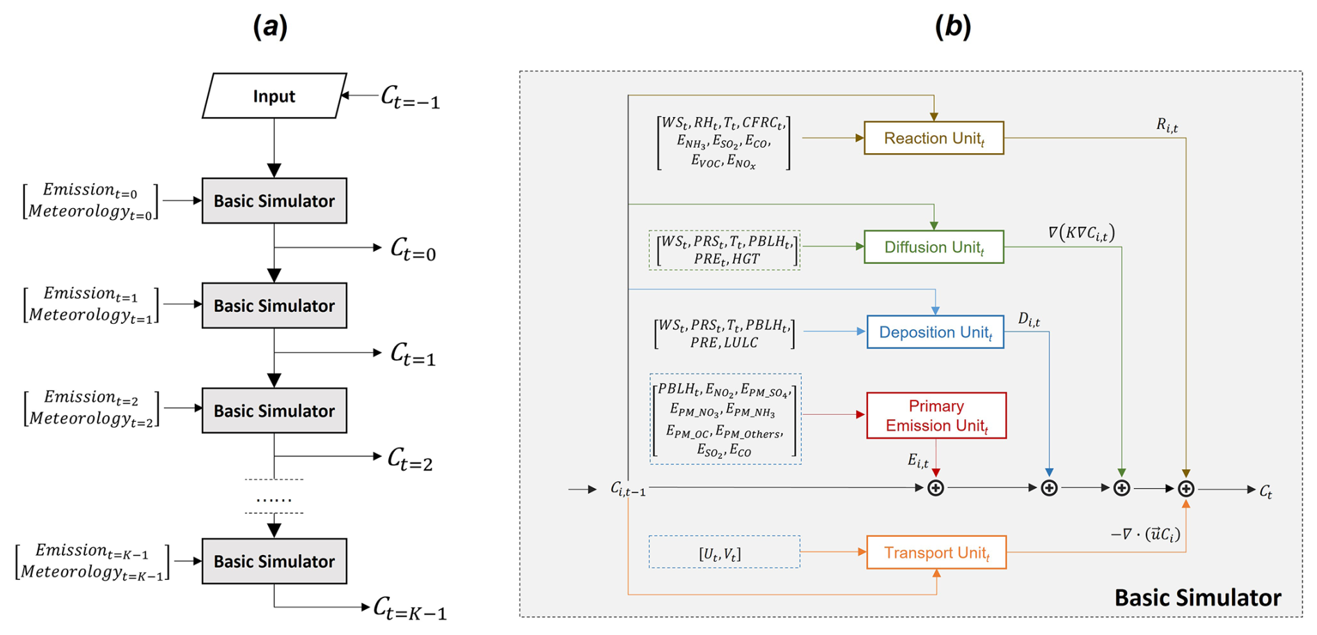
Figure 1 (a) General model workflow, and (b) the basic simulator module structure at the time step t of the deep learning simulation model FastCTM, designed according to Eq. (1). Arrows and boxes with different colours represent calculation modules of different atmospheric physical and chemical processes.

The FastCTM model uses the basic simulator module (Fig. 1a) recursively for hourly simulations, using output air pollutant concentrations from one step as input to the next step basic simulator. In contrast to directly learning spatiotemporal correlations of predictand itself as in most previous studies (Wang et al., 2018; Shi et al., 2017), the basic simulator (Fig. 1b) is formulated following the atmospheric physical and chemical equations and constraints shown in Eq. (1), and is composed of five modules to respectively represent the physics-chemical processes to improve the model performance. The modules for each of the five processes in the basic simulator are described in the following section. The time step used in FastCTM was 60 s.

2.2.2 Primary Emissions Module

Primary pollutants are assumed to be directly emitted into the atmosphere and instantly well-mixed within the PBL. Therefore, hourly enhancement of air-pollutant concentrations caused by primary emissions could be described in the following Eq. (3).

$$\begin{array}{}\text{(3)}& E_{m,n,i,t}={\displaystyle \frac{\mathrm{1000}\times {\mathrm{PE}}_{m,n,i,t}}{\mathrm{PBLH}\times \mathrm{d}x\times \mathrm{d}y}}\end{array}$$

Where $E_{m,n,k,t}$ refers to the concentration changes contributed by primary emissions at spatial coordinate (m,n) for species i at time t. The ${\mathrm{PE}}_{m,n,i,t}$ is the corresponding total primary emissions within the grid cell per second, which has a unit of g s⁻¹. Considering that the cell size in the FastCTM is 12 km by 12 km, we have dx = 12 000 and dy = 12 000 in this study. The boundary layer height PBLH, is also in the unit of meters (m). Therefore, the resulting air pollutant concentration increases by primary emission $E_{m,n,i,t}$ has a unit of µg m⁻³.

2.2.3 Horizontal Transport Module

In the FastCTM, horizontal transport usually has a significant influence on air quality variations (Lang, 2013). In CMAQ, the regional transport is generally represented by the divergence of the product of wind field and air pollutant species as in Eq. (1), inferred from continuity equations and convection equations (Michalakes et al., 2001; Byun and Schere, 2006). By decomposing the air mass movement into two orthogonal directions of east–west (x) and north–south (y), they could be rewritten in the form shown in Eq. (4),

$$\begin{array}{}\text{(4)}& \mathrm{\nabla }\cdot \left(\mathit{u}{C}_i\right)={\displaystyle \frac{\partial \left(C_{i}U\right)}{\partial x}}+{\displaystyle \frac{\partial \left(C_{i}V\right)}{\partial y}}\end{array}$$

Where the wind field is represented as u, which is then decomposed into U and V, respectively, in the x and y directions.

In the deep learning framework, the partial equation in Eq. (4) could be rewritten in a discrete form as convolution operations and inner product calculations as shown in Eq. (5) with a finite difference method. The convolutional kernels of W_x and W_y were defined in an upwind scheme as shown in Eqs. (6) and (7). With the scheme, this transport module itself is mass-conserved, even though FastCTM is not mass-conserved as a whole.

$$\begin{array}{}\text{(5)}& {\displaystyle }\mathrm{\nabla }\cdot \left(\mathit{u}{C}_i\right)={\displaystyle \frac{W_x\cdot \left(C_i\times U\right)}{\mathrm{d}x}}+{\displaystyle \frac{W_y\cdot \left(C_i\times V\right)}{\mathrm{d}y}}\text{(6)}& {\displaystyle }{W}_x=\left\{\begin{array}{ll}\left[\begin{array}{ccc}-\mathrm{1}& \mathrm{1}& \mathrm{0}\end{array}\right]& \text{if}U<\mathrm{0}\\ \left[\begin{array}{ccc}\mathrm{0}& -\mathrm{1}& \mathrm{1}\end{array}\right]& \text{if}U\ge \mathrm{0}\end{array}\right.\text{(7)}& {\displaystyle }{W}_y=\left\{\begin{array}{ll}\left[\begin{array}{c}\mathrm{0}\\ \mathrm{1}\\ -\mathrm{1}\end{array}\right]& \text{if}V<\mathrm{0}\\ \left[\begin{array}{c}\mathrm{1}\\ -\mathrm{1}\\ \mathrm{0}\end{array}\right]& \text{if}V\ge \mathrm{0}\end{array}\right.\end{array}$$

2.2.4 Diffusion Module

Diffusion involves the physical and chemical processes that disperse pollutants in the atmosphere. It is influenced by meteorological conditions, i.e. atmospheric stability and humidity, and surface features, i.e., land terrains and vegetation (Jiang et al., 2021). The turbulence diffusion process ∇(K∇C_i) in Eq. (1) helps the spread of pollutants in the atmosphere. It is expressed as the second-order deviation of species concentrations as shown in Eq. (8). They could also be discretized to convolutional operations with the finite difference method as shown in Eq. (9), just like that in the horizontal transport process module.

$$\begin{array}{}\text{(8)}& {\displaystyle }\mathrm{\nabla }\left(K\mathrm{\nabla }{C}_i\right)={\displaystyle \frac{\partial }{\partial x}}\left(K{\displaystyle \frac{\partial C_i}{\partial x}}\right)+{\displaystyle \frac{\partial }{\partial y}}\left(K{\displaystyle \frac{\partial C_i}{\partial y}}\right)\text{(9)}& {\displaystyle }\mathrm{\nabla }\left(K\mathrm{\nabla }{C}_i\right)={\displaystyle \frac{W_x\cdot \left(K\times W_x\cdot C_i\right)}{\mathrm{d}x\times \mathrm{d}x}}+{\displaystyle \frac{W_y\cdot (K\times W_y\cdot C_i)}{\mathrm{d}y\times \mathrm{d}y}}\text{(10)}& {\displaystyle }K={\mathrm{Encoder}}_K\left(\left[T,\mathrm{RH},\mathrm{PRS},\mathrm{PBLH}\right]\right)\end{array}$$

The turbulent diffusivity K is closely related to the meteorological conditions of the atmosphere and is simulated with an encoder module Encoder_K (Eq. 10). The input variables of the Encoder_K include temperature T, humidity RH, surface pressure PRS, and boundary layer height PBLH. The Encoder_K is determined to be a grid-to-grid regression model based on the Unet$++$ model with a nested structure (Zhou et al., 2018; Ronneberger et al., 2015). The Encoder_K model consists of 5 layers with each layer respectively composed of 16, 32, 64, 128 and 256 filters.

2.2.5 Chemical Reaction Module

Reduced-form models like InMAP (Tessum et al., 2017) and EASIUR (Gentry et al., 2023) focus on annual-average exposure, while FastCTM provides hourly-resolved simulations critical for real-time management. FastCTM quantifies hourly contributions from individual processes (transport, chemistry, emissions) via its modular design, rather than aggregating source impacts in reduced-form models (e.g., EASIUR's source-receptor matrices). Furthermore, FastCTM explicitly couples meteorology (PBLH, T, RH) with chemistry, whereas InMAP/APEEP (Muller and Mendelsohn, 2007) assume static meteorology, which limits their utility in capturing diurnal or synoptic-scale variations. Specifically, the air pollutant concentration changes caused by chemical reactions are represented in the following Eq. (11). In the equation, the rate of chemical reaction of species i is expressed as the product of a rate constant k and a term that is dependent on the concentrations of its reactants j (Carter, 1990; Carter and Atkinson, 1996).

$$\begin{array}{}\text{(11)}& {\displaystyle }{R}_{m,n,i,t}=k_{m,n,i,t}\times f\left(C_{m,n,j,t}\right)\text{(12)}& {\displaystyle }{k}_i={\mathrm{Encoder}}_k\left(\left[T,\mathrm{RH},\mathrm{PRS},\mathrm{WS},\mathrm{PRE},\mathrm{CFRAC}\right]\right)\end{array}$$

The reaction kinetics constant k is generally temperature-dependent. They could also be related to atmospheric pressures and moisture humidity in some reaction processes. Therefore, the reaction rate constant k is simulated using a spatial encoder function Encoder as shown in Eq. (12), which has the same structure as that of diffusion encoder modules (Eq. 10). There are 6 input variables of the Encoder_k including T, RH, PRS, WS, RN and CFRAC. The concentration processor f is designed as a simple multi-layer convolutional network with a kernel size of 1 to represent high-order and complex relations among different reactants.

2.2.6 Deposition Module

Air pollutant deposition refers to the process by which atmospheric pollutants are transferred to Earth's surfaces (land, water, vegetation) or removed from the air. This phenomenon plays a critical role in environmental pollution dynamics and ecosystem impacts. The deposition was closely influenced by meteorological conditions and surface characteristics (Janhäll, 2015). For example, high wind disperses pollutants, while turbulence enhances dry deposition. Forests and crops act as sinks due to large surface areas for adsorption. Air quality changes due to the deposition process are expressed linearly as the product of the deposition rate d and the corresponding air pollutants concentrations C, as shown in Eq. (13). The constant d is closely related to the current and previous meteorological conditions, terrains, and underlying land cover types. Therefore, they are all simulated with an Encoder module as shown in Eq. (14).

$$\begin{array}{}\text{(13)}& {\displaystyle }{D}_{m,n,i,t}=d_{m,n,i,t}\times C_{m,n,i,t}\text{(14)}& {\displaystyle }d={\mathrm{Encoder}}_d\left(\left[\mathrm{WS},\mathrm{RH},\mathrm{RN},\mathrm{HGT},\mathrm{LULC}\right]\right)\end{array}$$

The model structure and parameter configurations are also the same as that of Encoder_K and Encoder_k. The input data variables of Encoder_d include WS, RH, RN, HGT and LULC.

2.3 Model Training

The FastCTM was programmed with Python 3 on the deep learning framework TensorFlow (Abadi et al., 2016). The model was trained with the WRF-CMAQ operational forecast data in China for 2018–2022. Considering that on each day we had 120 h forecasts with a spatial coverage of 426 × 372 grid cells (each with a size of 12 × 12 km²) for 9 meteorological variables and I=10 air pollutant variables, the total training dataset has a size of $\mathbf{TD}={\mathbf{R}}^{\mathrm{1826},\mathrm{120},\mathrm{426},\mathrm{372},\mathrm{19}}$, where 1826 represents the total counting days from 2018 to 2022. Since the model was set to predict 24 h PM_2.5 concentrations from 1 h input data, the total input sequence length was 25 h in each training step. Besides, the size M×N of the input data X_t to FastCTM was decided to be 150 × 150, equal to an area of 1800 × 1800 km² in 12 km resolution. Therefore, the input batch data for FastCTM in each step should be the size of $\mathbf{BD}={\mathbf{R}}^{b,\mathrm{25},\mathrm{150},\mathrm{150},\mathrm{19}}$, where b is the batch size (determined as 1 in this study). The input data BD are randomly sliced from the whole training dataset TD in each training iteration, indicating each BD represents different spatial and temporal coverages. The random sampling tactics help the model learn inherent physical and chemical principles rather than just statistical spatiotemporal autocorrelations using data in a constant spatial area (Xing et al., 2022). Besides, the spatio-temporal random samples contain varied emissions, which would improve FastCTM adaptation to changing emission levels.

Even though five modules are defined in FastCTM, individual processes are not trained separately. The model was trained as a whole with hour-to-hour air pollutant concentrations, while each process could learn its parameters under the constraints of its dedicated formulation. Specifically, FastCTM was tuned to minimize the loss function L, which was determined to be L2 loss (Bühlmann and Yu, 2003) of the regularized mean squared error (MSE) as shown in Eq. (15). The model was optimized using the Adam optimizer (Kingma and Ba, 2014).

$$\begin{array}{}\text{(15)}& L={\displaystyle \frac{\mathrm{1}}{J\times N\times M\times I}}\sum _{t=\mathrm{1}}^J\sum _{m=\mathrm{1}}^M\sum _{n=\mathrm{1}}^N\sum _{i=\mathrm{1}}^I{\left(C_{m,n,i,t}-{\stackrel{\mathrm{̃}}{C}}_{m,n,i,t}\right)}^{\mathrm{2}}\end{array}$$

The learning rate was set to be 0.001, and the batch size to be 1. The FastCTM model was trained on one entry-level professional acceleration card of NVIDIA A40 with a running time of 10 h for every 10 000 iterations. A total of 300 000 iterations were performed until the remaining model loss stabilized.

2.4 Model Evaluation

FastCTM was assessed against CMAQ simulations using the same input emission data and meteorological fields. Starting from 00:00 local time on each day, the CMAQ model simulated 120 h forecasts in one cycle. There are 139 cycles in the evaluation year of 2023 due to data unavailability in the remaining days. The FastCTM model generated 119 h forecasts using a 1 h initial input condition. The 119 h forecasts in the leading hours from 2 to 120 by the two models were compared regarding to the corresponding leading time. For example, when we had a 120 h forecast starting at 00:00 on 1 January 2023 at Beijing Local Time (BLT), the data of 00:00 on 1 January 2023 were fed into FastCTM to get the 119 h forecasts until 23:00 on 5 January. The 10 species forecasts by FastCTM were compared against the CMAQ forecasts at each corresponding hour. The metrics of root mean square error (RMSE) and coefficient of determination (R²) were calculated daily in each of 119 leading hours on the difference in each of the 158 742 grid cells between CMAQ and FastCTM. Therefore, metrics of R² and RMSE were obtained on each lead hour on each day of the independent test year of 2023. The statistical values on each day are then averaged for the same leading hour for comparison.

The FastCTM was also assessed in terms of sensitivity analysis to emission inputs and meteorological fields. For meteorological variables, responses of six criteria pollutant concentrations to T, WS, and PBLH were calculated. For emissions, responses to paired variables of SO₂/NH₄ and NO_x/VOC were calculated. Besides, FastCTM's capability to simulate responses to emission changes was also evaluated by comparing with CMAQ simulations in 11 emission-intervention scenarios. Finally, the contributions of five internal processes of transport, diffusion, emission, reaction, and deposition were also analyzed and discussed for an example pollution episode.

3 Results

3.1 Forecast Performance by FastCTM

FastCTM has exhibited strong, stable performance in reproducing CMAQ forecasts over the 119 h forecast period evaluated for 2023 (Fig. 2). The average RMSE values for six criteria pollutants of PM_2.5, PM₁₀, SO₂, NO₂, CO, and O₃ are, respectively 9.1, 11.9, 4.4, 4.0, 48.9 and 10.9 µg m⁻³. For R² values, they are 0.8, 0.81, 0.8, 0.83, 0.9 and 0.7. As for PM_2.5 components, RMSE values are 1.68, 2.68, 1.52, 1.98 and 4.25 µg m⁻³, respectively for SO${}_{\mathrm{4}}^{\mathrm{2}-}$, NO${}_{\mathrm{3}}^{-}$, NH${}_{\mathrm{4}}^{+}$, organic matters and other inorganic components, while the R² values are 0.72, 0.6, 0.3, 0.83 and 0.68. Compared to the ∼ 5 ppb (∼ 10.5 µg m⁻³) in the previous study by Xing et al. (2022), the FastCTM model has similar RMSE values in forecasting O₃. To test the influences of initial conditions on FastCTM long-term simulations, FastCTM forecasts using zero values as input air quality data were almost the same as those using ordinary input in the long leading hours. Results indicating that FastCTM simulations in long leading hours are not affected by initial conditions (Fig. S5 in the Supplement), just like deterministic CTMs (such as CMAQ). In other words, the insensitivities of FastCTM to initial conditions indicate that it has well learned and encoded the most physical and chemical principles in CMAQ CTM, rather than just spatio-temporal correlations among air quality sequences.

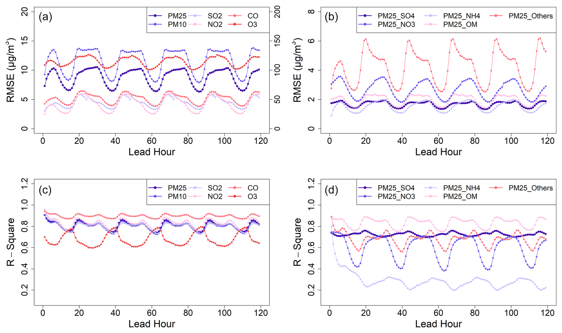
Figure 2 The evaluation performances of FastCTM forecasts against CMAQ forecasts in 2023. Panels (a) and (b) respectively show RMSE values of criteria pollutants and the PM_2.5 components. Panels (c) and (d) show R² values. It should be noted that the RMSE value of CO corresponds to the right axis in (a).

Hourly RMSE values show clear diurnal variation with higher RMSE values in the nighttime than that in the daytime, which could be due to higher hourly concentrations of air pollutants in the nighttime, except for O₃ (Fig. S6 of the Supplement). Consistency between CMAQ and FastCTM, as characterized by R², is lower in the daytime. Since the FastCTM is a 2-D model only considering atmospheric processes within the boundary layer, lower consistency with the CMAQ model during daytime, possibly due to more vigorous vertical mixing. Strong vertical mixing of air pollutants to the height above PBLH has been found (Li et al., 2017; Tang et al., 2016), which may not be fully represented in FastCTM. It is important to note that the relatively low R² values observed for NH${}_{\mathrm{4}}^{+}$. While CMAQ explicitly resolves NH${}_{\mathrm{4}}^{+}$ formation reactions, FastCTM does not explicitly encode these pathways. Instead, the neural network implicitly learns relationships between NH${}_{\mathrm{4}}^{+}$ and precursor emissions (NH₃, NO_x, SO₂) and meteorological variables (e.g., temperature, humidity). This simplification omits acid-base equilibria and aerosol thermodynamics, which are critical for partitioning NH${}_{\mathrm{4}}^{+}$ between gas and particle phases. The low R² for NH${}_{\mathrm{4}}^{+}$ primarily reflects FastCTM's simplified chemical mechanism in this part, which could be improved by adding related species in the simulation.

The spatial distributions of the mean absolute error (MAE) and the normalized mean absolute error (NMAE) are presented in Fig. 3. For all six pollutants under consideration, MAE values tend to be higher in polluted areas. In polluted environments, there are often multiple sources of emissions, complex chemical reactions, and variable meteorological conditions that can lead to greater discrepancies between the predicted concentrations of the two models. Conversely, the NMAE values exhibit an opposite trend, being lower in polluted areas. In these regions, the NMAE values typically hover around 0.2, in contrast to the relatively higher values of approximately 1 in cleaner areas. The NMAE is a normalized metric that takes into account the magnitude of the actual pollutant concentrations. A lower NMAE in areas with high pollution levels suggests that the FastCTM model is effectively capturing the overall magnitude and trends relative to the reference CMAQ simulation. The Air quality forecasts starting from 00:00 a.m. on 4 March 2023 (Fig. S7 in the Supplement) demonstrate FastCTM's strong capability in modelling the complex spatio-temporal changes in a large spatial domain and over a relatively long period and a large area.

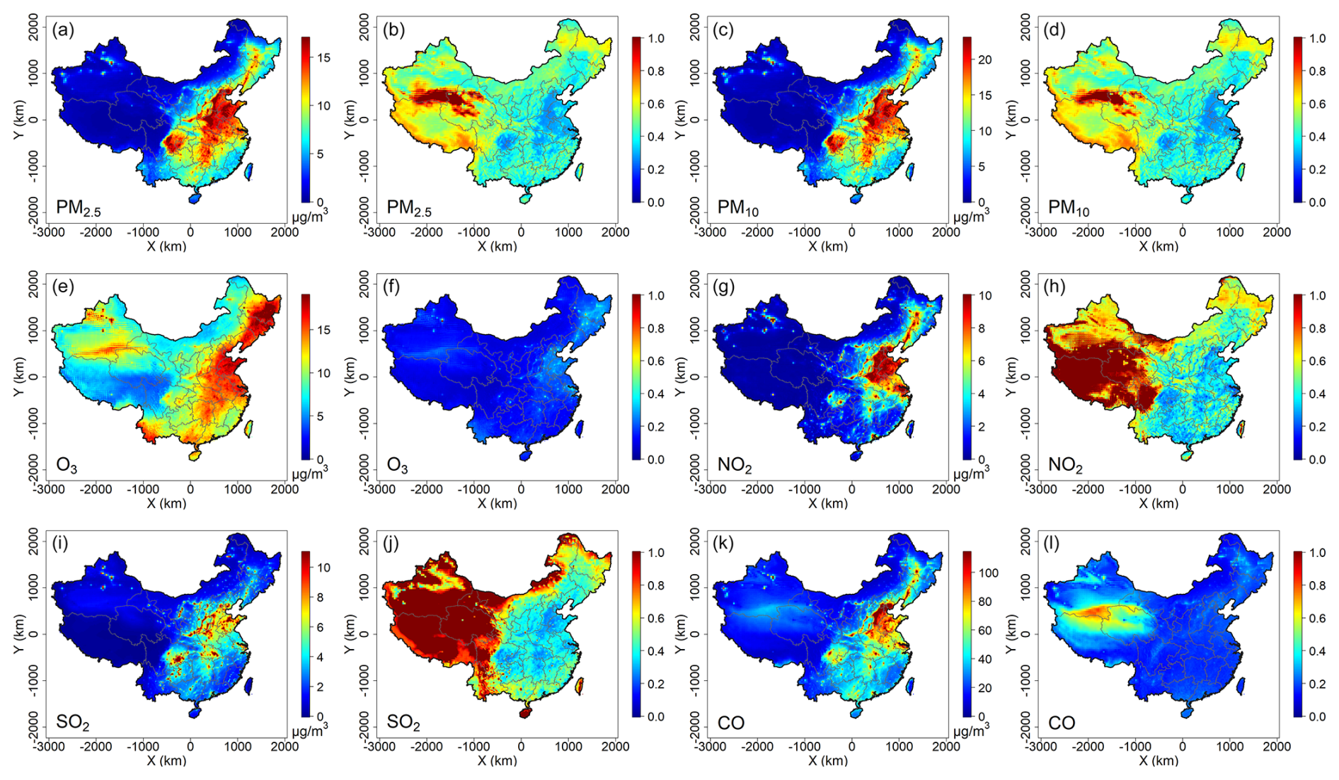
Figure 3 Spatial distribution of mean absolute error (a, c, e, g, i, k) and normalized mean absolute error for the six criteria pollutants (b, d, f, h, j, l) of FastCTM compared with CMAQ in 2023.

Defining the warm season as the months from April to September and the winter and cold season as the remaining months, the FastCTM model exhibited comparable performances. As shown in Fig. 4 (with detailed information in Fig. S8 in the Supplement), the coefficient of determination R² values for the six criteria pollutants were 0.82, 0.8, 0.8, 0.82, 0.91, and 0.7 in the warm season, and 0.8, 0.79, 0.78, 0.83, 0.88, and 0.68 in the cold season, respectively. To assess the performance variations of FastCTM across different spatial locations, comparative evaluations were carried out in urban and rural areas as well as in inland and coastal regions. Generally, FastCTM demonstrated slightly higher accuracies in rural areas compared to urban areas (as presented in Fig. S9 in the Supplement). This outcome is reasonable given the more intricate emission and chemical processes prevalent in urban settings (Guo et al., 2014). Similarly, FastCTM exhibited comparable performances in inland areas to those in coastal areas, except for PM_2.5 and PM₁₀ (Fig. S10 in the Supplement).

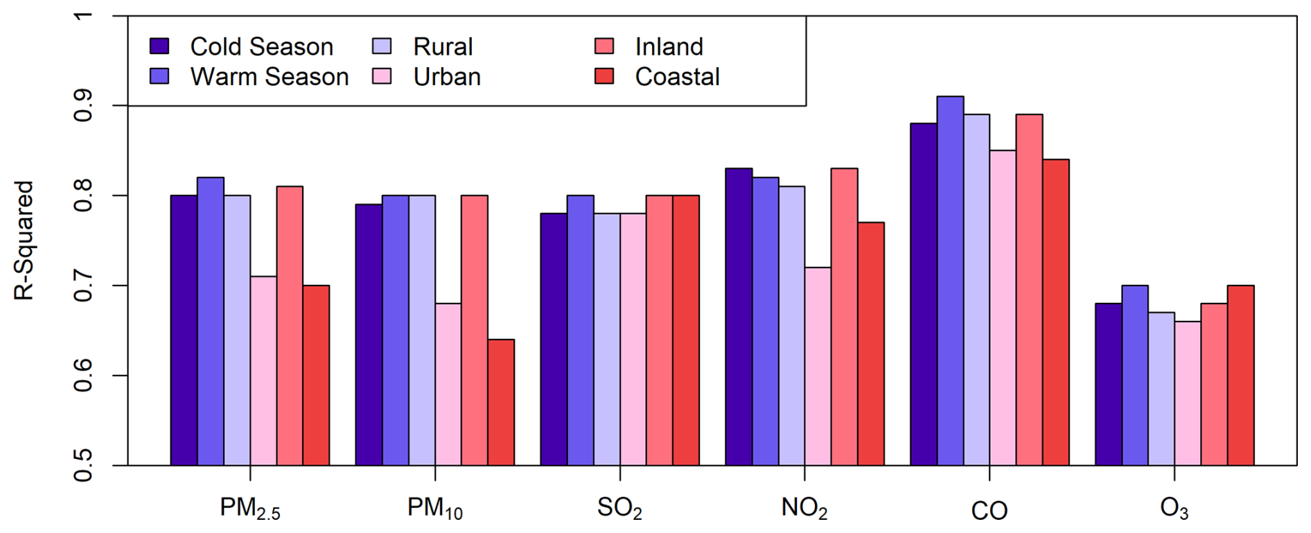
Figure 4 The mean evaluation R² values for all 119 leading hours of FastCTM forecasts in warm/cold seasons, rural/urban areas, and coastal/inland areas.

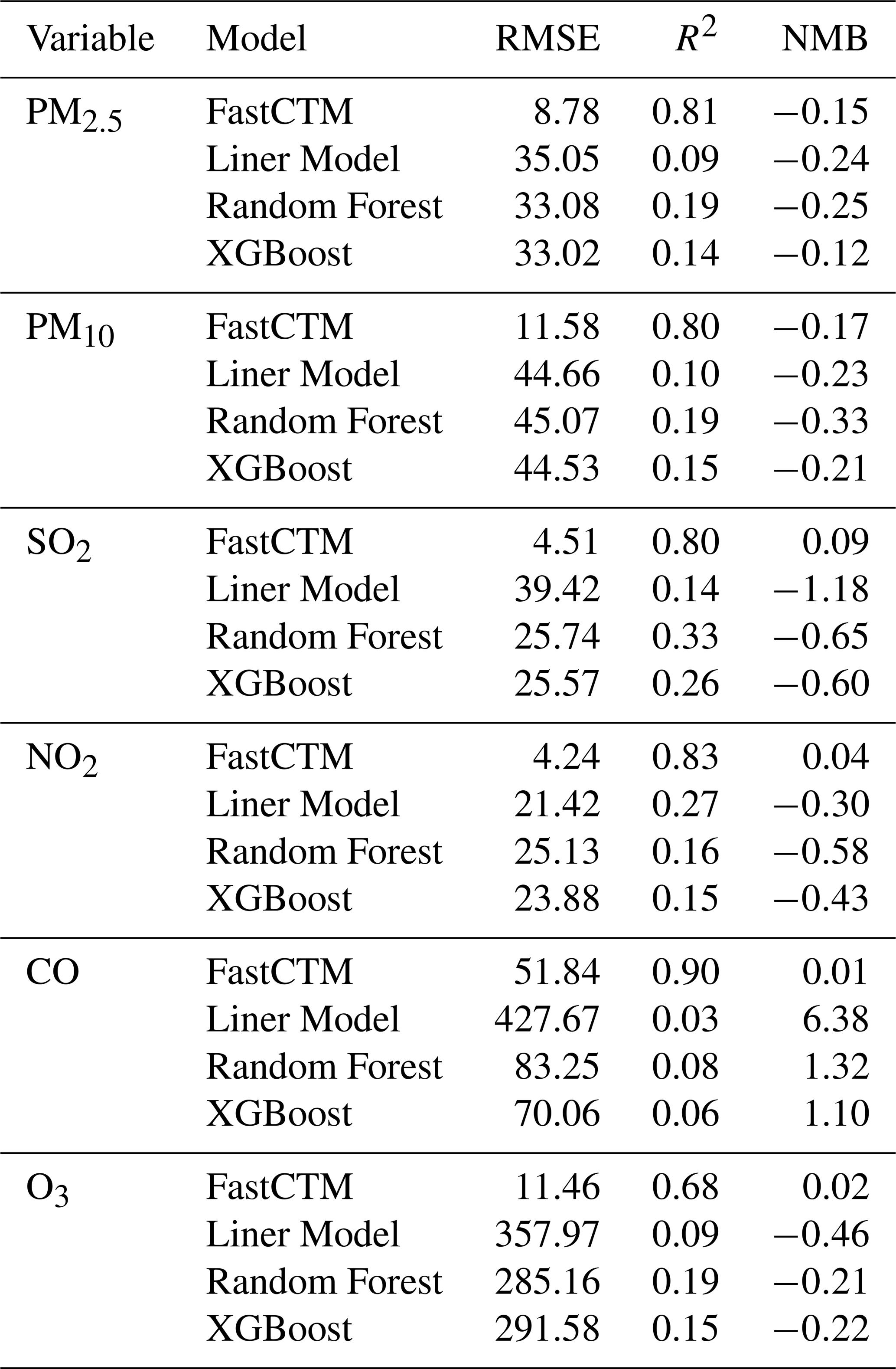
To validate the FastCTM model, three land use regression (LUR) models were constructed, namely the linear regression model, the random forest model (with the number of trees set at 500), and the XGBoost model (with the booster specified as gbtree). These LUR models were developed using the same input meteorological data, emissions, and geophysical variables as FastCTM to ensure fair comparison. When compared with the FastCTM model, the performance of the LUR models was found to be significantly inferior, as demonstrated in the Table 1 and Figs. S10–S12 in the Supplement. For example, R² values for FastCTM range from 0.68–0.90, whereas the LUR models only achieve 0.06–0.33. This outcome is anticipated when we consider the complex nature of air quality dynamics in predicting future air quality. Air quality is not a static entity, but it varies both spatially and temporally, determined by the joint effects of local emissions, meteorological conditions, and surface features, etc. For instance, the transport of air pollution is a highly dynamic process that hinges on wind fields and air pollution concentrations in a reciprocal manner. The wind direction and speed dictate the trajectory along which pollutants travel, while the existing pollutant concentrations in different regions influence the overall dispersion and mixing patterns. LUR models, which on the other hand predominantly rely on local input data (Wong et al., 2021; Cheng et al., 2021), struggle to capture these intricate, non-local interactions. They cannot account for the far-reaching effects, such as wind-driven pollutant transport and the temporally accumulated changes in air quality over larger geographical areas. As far as we know, LUR models have been mostly applied in predicting air pollution fields in retrieval given corresponding air quality observations as training and constrained input data. They have been seldom used in air quality forecasts and simulations, as we have demonstrated with the FastCTM model.

Table 1 Performance metrics of LUR models and FastCTM compared against CMAQ.

Annually, the daily air quality typically exhibits similar fluctuations to those in other years, which can be primarily attributed to the cyclical nature of meteorological conditions and pollutant emission patterns. The FastCTM model was trained using a comprehensive dataset spanning five years, from 2018 to 2022. In light of this, it was crucial to rule out the possibility that the model was merely reproducing historical averages during the test year of 2023. To this end, the daily national average concentrations of PM_2.5 and O₃ in 2023, as predicted by FastCTM, were meticulously compared with those simulated by CMAQ in the same test year, as well as with the CMAQ forecasts from the training years of 2018–2022. As illustrated in Fig. 5, the predictions made by FastCTM in 2023 align more closely with the actual CMAQ forecasts for that year, with R²=0.94 and 0.72, respectively, for PM_2.5 and O₃, rather than with the forecasts generated from the training data of 2018–2022, with R²=0.54 and 0.59. The NMB was also lower between FastCTM and CMAQ for the same year, 2023. These results not only validate the adaptive learning capabilities of the FastCTM model but also indicate that the model is not using a simplistic approach of averaging concentrations from the previous five years based on time of day. Hourly time series plots of air pollutant concentrations (Fig. S6 in the Supplement) further demonstrate that FastCTM appears to incorporate real-time meteorological feedback, adjust for shifts in emission patterns, and leverage its learned relationships to provide more accurate and contemporaneous predictions.

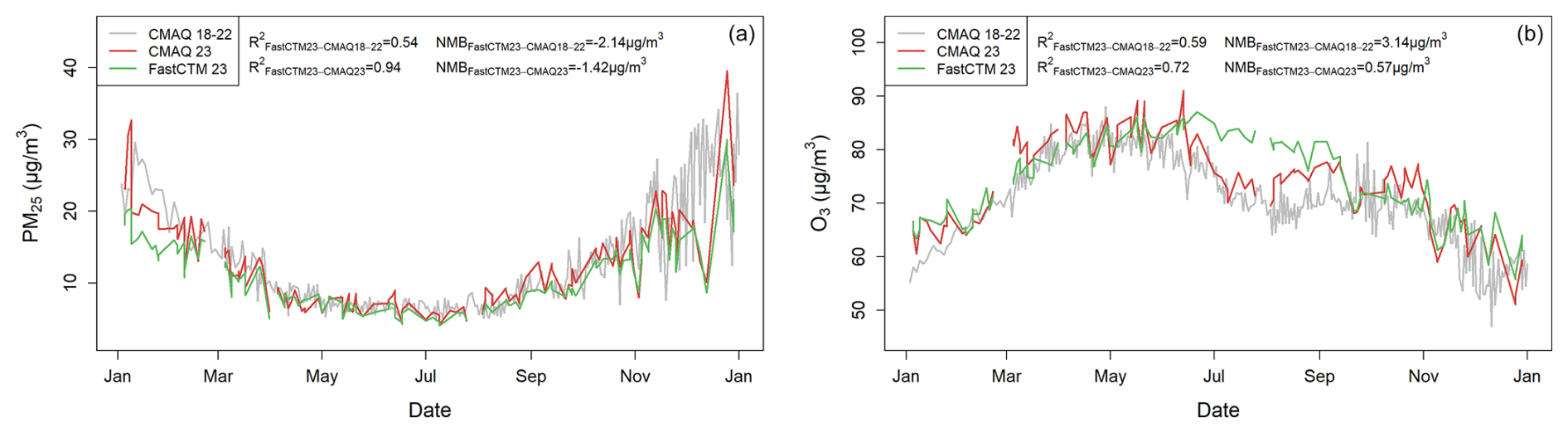
Figure 5 The daily FastCTM forecasts compared with CMAQ forecasts, respectively, in the training period of 2018–2022 and the evaluation period of 2023 for (a) PM_2.5 and (b) O₃. The gaps for FastCTM and CMAQ in 2023 are due to data unavailability these days.

3.2 Sensitivity Analysis with FastCTM

The FastCTM model was trained with 5-year meteorological and air quality simulations by WRF-CMAQ. These simulations used an emission inventory that was identical for every year. In this condition, the FastCTM model has learned the relationships between the air quality and varied meteorology with fixed emissions input. Considering that the FastCTM model has exhibited high accuracy in an independent evaluation year 2023, when new meteorological fields are fed into FastCTM, the deep learning model should be able to simulate responses of air pollutant concentrations to meteorological variables. However, for the response of air pollutant concentrations to emissions, the training data do not contain relationships between inter-annual varied emissions and air quality under the condition of the same annual meteorological fields. Therefore, it is less expected for FastCTM to simulate reliable and correct response relationships between emissions and air quality. To validate these analyses, we calculated the sensitivities of simulated air pollutant concentrations to changes in meteorological variables and emissions.

3.2.1 Response of Air Pollutant Concentration to Meteorology

The responses of six criteria pollutants to meteorological changes simulated by FastCTM are evaluated as exhibited in Fig. 6. For ground-level temperature (T) elicited a distinct response in O₃ concentrations compared to the other five criteria pollutants. O₃ concentrations have slight negative responses to T in January, as shown in Fig. 6a, which is probably because higher temperatures increase NO? emissions, enhancing dilution. O₃ concentrations had the strongest positive responses in August among six pollutants, which is consistent with previous observation-based studies (Flaum et al., 1996). The O₃ had larger sensitivities when the air temperature was higher. The gaseous pollutants of CO, NO₂, and SO₂ show the strongest positive response to temperature, which could be caused by the shift of chemical equilibrium towards the higher release of these gaseous pollutants (Bassett and Seinfeld, 1983; Cox, 1982). The particulate matter pollutants, especially PM₁₀, have the weakest responses among six pollutants. Considering that there are dominating proportions of chemically inert species in particulates, the weak responses of PM_2.5 and PM₁₀ are expected.

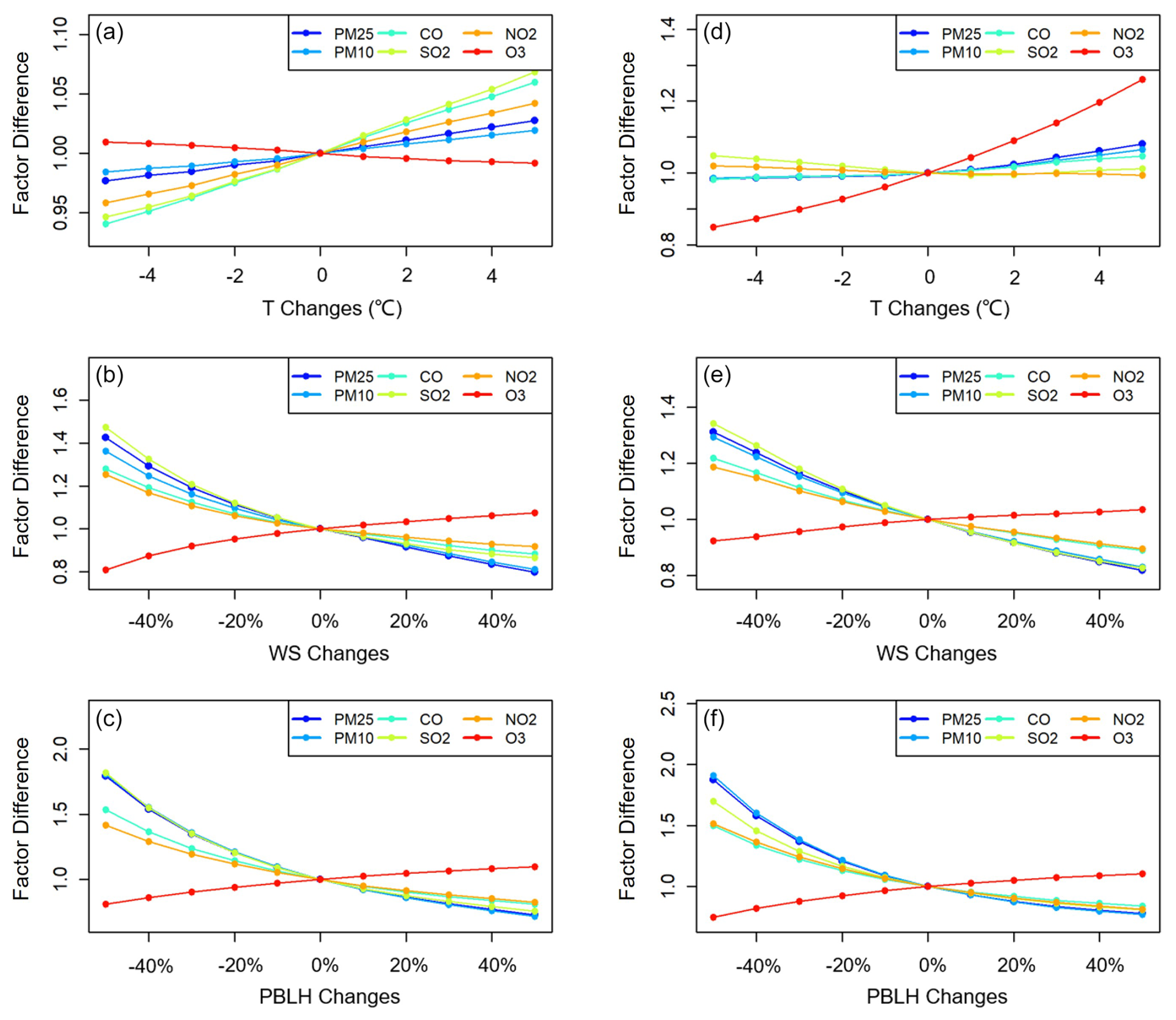
Figure 6 The FastCTM predicted air pollutant percentage changes in response to changes of T, WS, and PBLH in Beijing on 2 January (a–c, respectively in the left column) and 1 August (d–f, respectively in the right column), 2023. The air pollutant concentrations are relative to those at the baseline meteorological conditions.

For the wind speed and PBLH, the responses of pollutants have similar patterns for the same pollutant. First, O₃ concentrations exhibited patterns opposite to other pollutants both in January and August. Higher wind speed would increase the dispersion and transport of air pollutants (Feng et al., 2015; Lv et al., 2017), resulting in lower pollution levels, so concentrations decrease as wind speed increases, except for O₃. The contradictory response of ozone and particulate matter concentrations to PBLH is consistent with the analysis results of multiple-year observations (Liu and Tang, 2024). Theoretically, the air pollutant concentrations should exhibit an inverse relationship between air pollution concentrations and PBLH. The actual air pollutant concentration changes simulated by FastCTM generally fit the theory that there are negative nonlinear effects with increasing PBLH. Meanwhile, the sensitivity is stronger when the PBLH is lower (Fig. 6e and f), which is consistent with previous observation-based analysis (Wang et al., 2019; Su et al., 2020). The totally different relationship of O₃ to wind speed and PBLH compared to other pollutants could be due to its high dependence on chemical precursors, such as NO_x and VOC. Concentrations of these precursors could have an inverse relationship with O₃ at specific locations. The FastCTM model itself is trained with multi-year CMAQ simulations, indicating that it is preconditioned on varied meteorological fields with the same atmospheric physical and chemical rules. Therefore, the sensitivity of air quality simulations to meteorological variations could be well learned, especially with the discipline-based model FastCTM.

3.2.2 Response of Air Pollutant Concentration to Emission

The sensitivity analysis with a “brute force” method can be carried out with the FastCTM model quickly due to its high computational efficiency on GPU. The responses of PM_2.5 concentrations to doubled emissions of SO₂, NO_x were explored in the winter month of January 2023 (Fig. 7). For doubled NO_x, the PM_2.5 concentrations exhibited positive responses in most areas of China as shown in Fig. 7a. The largest increases occurred in North China, Heilongjiang province in Northeast China, the Yangtze River Delta, and Sichuan province. In these places, the NO_x emissions are relatively large. For doubled SO₂, PM_2.5 concentrations increased in almost all of China as shown in Fig. 7b. The response was larger in North China, Northeast China and the Sichuan basin. The PM_2.5 responses simulated by FastCTM were generally consistent with previous studies (Li et al., 2022).

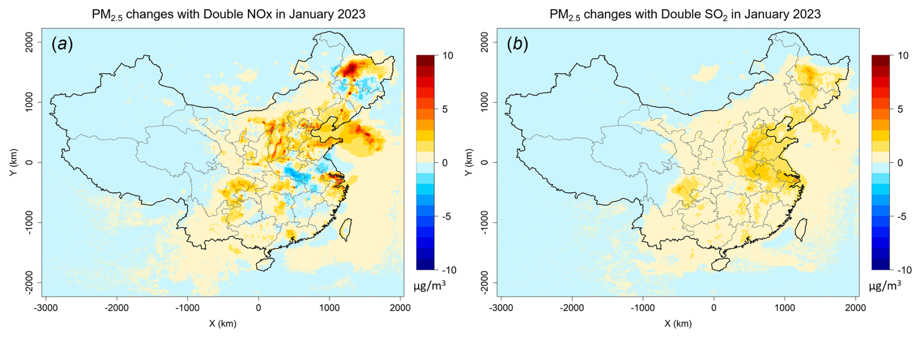
Figure 7 Average predictions of PM_2.5 concentrations in 5 lead-days with doubled emissions in January 2023. Panel (a) refers to predictions with doubled NO_x, and (b) refers to double SO₂.

As for ozone, its responses to doubled NO_x and VOC are explored as shown in Fig. 8. For NO_x emission, decreases in O₃ concentrations in polluted regions like North China, the Yangtze River Delta, and other highly industrial regions are well captured by FastCTM. The response is reasonable considering that these regions are generally abundant with NO_x emissions and at VOC-limited conditions. Doubling VOC emissions leads to a significant decrease in O₃ (Fig. S14 in the Supplement), since increased VOC would consume more O₃ in these regions. The spatial patterns of O₃ responses to NO_x and VOC are similar to a previous deep learning study trained by emission-controlled simulation data (Xing et al., 2022). However, due to the complex speciation of VOC emissions that is simplified in the FastCTM, uncertainties for responses of O₃ to VOC should be noted.

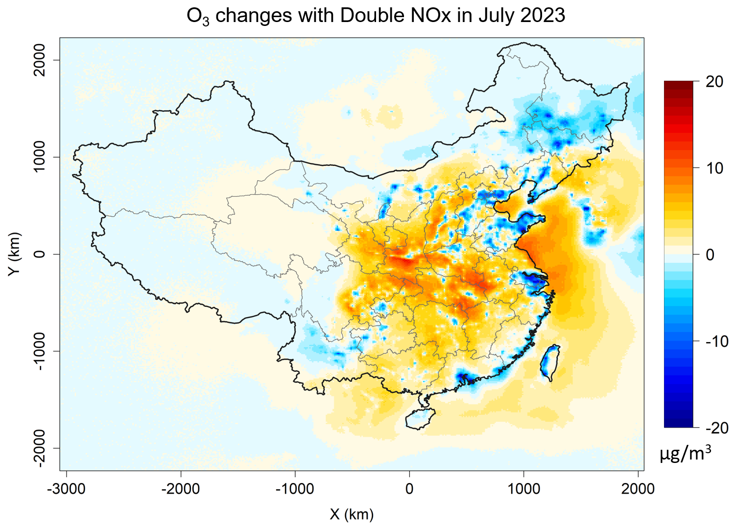
Figure 8 Average predictions of hourly O₃ concentrations in 5 lead-days with doubled NO_x emissions in July 2023.

The sensitivities of FastCTM simulations to emission interventions were contrasted with those of CMAQ. Specifically, CMAQ was employed to simulate 11 emission scenarios over the two-month periods of January and July 2019 in Southwest China (Huang et al., 2022). The alterations in emissions relative to the base case are presented in Table 1. Among these scenarios, 10 involved reduced emissions of major species, with only the no-control scenario exhibiting increased emissions. Utilizing the identical emissions and meteorological data, FastCTM also conducted simulations, which were then compared to those of CMAQ. For the 11 scenarios in question, the changes in air pollutant concentrations relative to the base case at the locations of 139 national air quality monitoring stations (Fig. S15 in the Supplement) were extracted and compared in the winter month of January 2019 (Fig. 9a) and in the summer month of July 2019 (Fig. 9b). The results indicated that, overall, the FastCTM simulations due to emissions changes were in good agreement with those of CMAQ, as reflected in two aspects. The correlation coefficient R values are around 0.9 for SO₂, NO_2, and O₃ in both summer and winter months. For PM_2.5 and PM₁₀, FastCTM exhibited higher consistency with CMAQ in July than in January, with R values around 0.6 for most cases. For CO, FastCTM has much better performance in January than in July, with R values of approximately 0.8 and 0.2. Considering that CO concentration changes are mostly due to physical dispersion and transport, the decreased performance is probably due to increased vertical mixing in summer, which is not fully represented in the 2D scheme of FastCTM. Specifically, in January 2019, except for NO₂, FastCTM responded to emission changes with an interquartile range (IQR, 25 %–75 % percentile) similar to that of CMAQ (Fig. S16). In July 2019, as depicted in Fig. S17, all the criteria pollutants except CO demonstrated a comparable degree of response to emission reductions.

Table 2 The emission change details of the emission scenarios.

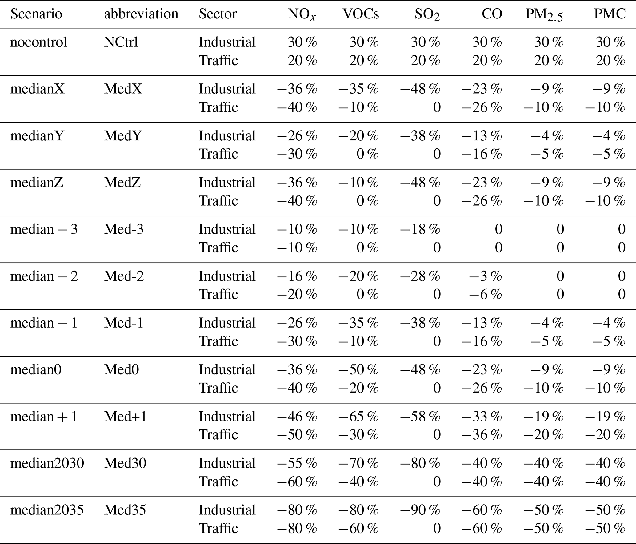
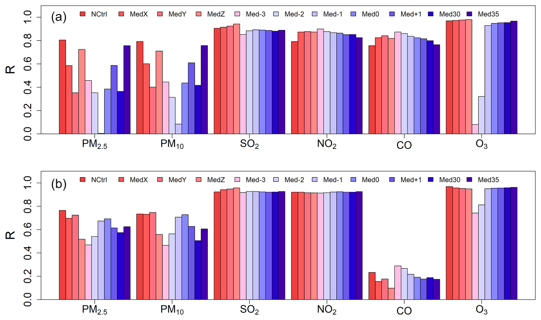
Figure 9 Correlation coefficient R for responses of FastCTM and CMAQ to different emission scenarios and different air pollutants in January 2023 (a) and July 2023 (b).

FastCTM model used a principles-constrained formulation framework. As shown in Eq. (4), atmospheric chemical reactions are in the Atkinson form, which independently estimates the reaction rate from meteorological conditions and polynomials of reactant concentrations in multiple powers. The principle-based formulation should be the reason for the relatively significant and reasonable response simulations of PM_2.5 and O₃ to precursor emissions, even though the FastCTM itself is not trained by emission-controlled CMAQ scenario simulations. The remaining uncertainties should be attributed to the reason that FastCTM only considered environmental chemical reactants in part, compared to that of the CMAQ model (Binkowski and Roselle, 2003).

3.3 Internal Processes Analysis with FastCTM

The FastCTM is a principles-guided deep neural network to individually simulate the dominant atmospheric physical and chemical processes as defined in Eq. (1). The processes are calculated numerically with critical parameters describing the processes being estimated by deep learning encoders. The hourly concentration changes equal the sum of the changes produced by each process. Figure 11 depicts an example during the nighttime of 13 January 2023, when hourly PM_2.5 concentration changes significantly. Between the two hours of 18:00 and 19:00, hourly PM_2.5 concentrations change markedly in neighbouring areas of Shandong, Hebei, and Henan provinces as shown in the red rectangle (denoted as Area A hereafter) in Fig. 11c. In this example, strong northern wind prevails, leading pollutants to move southward. For PM_2.5 concentration changes caused by primary emissions (Fig. 8d), it is determined by the primary emission and the mixing volumes determined by PBLH. PM_2.5 changes are mostly determined by the transport process (Fig. 11e) as its spatial pattern most closely resembles total PM_2.5 concentration changes. In the transport process, air pollutants move from one area to another, determined by the wind fields as shown in Eq. (4). When the northern clean air prevails as in Area A, changes should be negative in the upstream direction and positive in the downstream direction. The transport process simulated by FastCTM sticks to this pattern. As known to us, the diffusion process will bring pollutants from a region of high concentration to one of low concentration. Its contribution is low as shown in Fig. 11f, which is reasonable considering the relatively large grid cell size of 12 km and short simulation period of 1 h. PM_2.5 concentration changes caused by the diffusion process constituted a small proportion compared to other processes. The activities of chemical reactions are determined by both meteorological conditions and related precursor concentrations. PM_2.5 contribution changes between T1 and T2 caused by chemical reactions are lower in the areas to the north of Area A because the cold and clean air in this area is not favourable for chemical reactions. The deposition is the dominant process that led to PM_2.5 concentration reductions where regional transport was not significant. In general, deposition rates were proportional to PM_2.5 concentrations as shown in Fig. 8h (Davis and Swall, 2006). It should be noted that FastCTM simulated air quality in a 2-D domain rather than in 3-D. The deposition may also include the vertical transport of air pollutants to the upper air above PBL (Zhao et al., 2020).

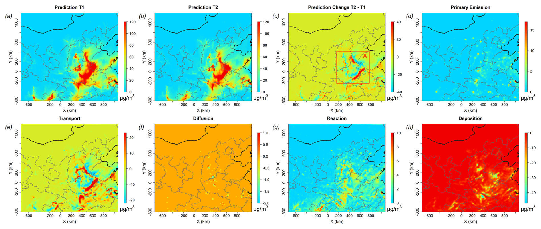
Figure 10 An example of the PM_2.5 concentration at T1 (18:00, a) and T2 (19:00, b) on 13 January 2023 (with the forecast leading time of 42 h) and hourly changes (c). Changes caused by each of the five dominant processes are depicted in (d)–(h).

Simulated contributions of five major processes to hourly PM_2.5 concentration changes are compared between FastCTM and CMAQ at 139 stations (Fig. S15) in the Sichuan-Chongqing region from 12 to 16 October 2024, as shown in boxplots of Fig. 11. Overall, the simulation results of the process contributions by FastCTM and its parent model CMAQ were relatively consistent. Higher degrees of consistency were found in simulations of emissions, advection processes, and diffusion processes between the two models. Contributions from chemical reactions of FastCTM exhibited overestimation compared to CMAQ, while contributions from deposition were underestimated. The differences in the simulated deposition and reaction contributions between the two models could be due to incomplete representation of influencing factors, given the complexity of the two processes. In general, the consistency between the two models provides confidence in the reliability of FastCTM for simulating and understanding the complex interplay of atmospheric processes that govern PM_2.5 levels.

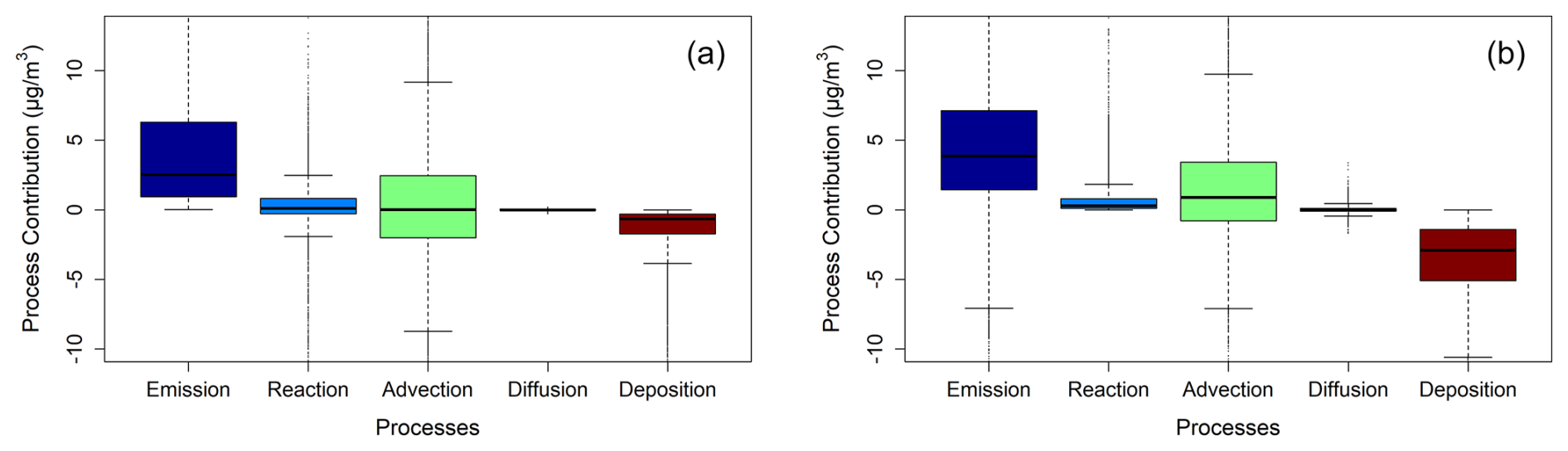
Figure 11 Boxplots of hourly PM_2.5 contribution changes from five major atmospheric processes at 139 evaluation stations from 13 to 16 October 2024, simulated by (a) CMAQ and (b) FastCTM.

4 Discussions

4.1 Model Accuracy and Uncertainty

One debatable concern is the accuracy of neural network (NN)-based components in integrated chemical transport models (CTMs) and the potential for amplified uncertainty when coupling multiple NN modules. Literature precedent suggests that individual NN emulators may exhibit lower accuracy compared to traditional physical parameterizations, but their integration could introduce unexplained uncertainties. This is a valid consideration that aligns with broader discussions in Earth system modeling about the trade-offs between computational efficiency and physical fidelity (Irrgang et al., 2021).

In FastCTM, we address this by adopting a principle-informed modular design where each module (transport, chemistry, deposition, etc.) is constrained by governing physical/chemical equations (e.g., Eqs. 3–14). This distinguishes it from unconstrained “black-box” NN models, as each process is guided by known atmospheric dynamics. For example, the transport module explicitly enforces mass conservation via upwind schemes (Eqs. 5–7), and the chemical reaction module links reaction rates to meteorological conditions (Eq. 12) based on kinetic theory. Our evaluation shows that FastCTM maintains high consistency with CMAQ across 119 h forecasts (Sect. 3.1), with R² values exceeding 0.8 for most pollutants, indicating that physical constraints effectively mitigate accuracy losses.

However, we acknowledge that uncertainty can accumulate when coupling modules, particularly for species involved in complex multi-process interactions due to limited chemical constraints in our current training datasets(e.g., NH${}_{\mathrm{4}}^{+}$, Sect. 3.1). This is partly due to simplifications in FastCTM's chemical mechanism, which omits some aerosol thermodynamics included in CMAQ. Future work will reduce such uncertainties by incorporating additional species (e.g., VOCs) and refining process formulations by adding CMAQ's integrated process rate (IPR) data for supervised training of individual modules.

4.2 Choosing Neural Network Components over Traditional Parameterizations

One question might arise about the utility of replacing non-bottleneck CTM components (e.g., deposition) with NN solvers, given the argument that traditional parameterizations may already be accurate and fast. This highlights a critical design choice in FastCTM: balancing computational efficiency with fidelity to the parent model (CMAQ).

It is important to note that even non-bottleneck components in traditional CTMs can benefit from NN acceleration in integrated simulations. For example, CMAQ's deposition module, while not a primary computational burden, relies on parameterizations based on similarity theory and limited flux measurements (Janhäll, 2015), which may oversimplify complex surface-atmosphere interactions (e.g., vegetation-specific uptake). NN-based parameterizations have shown promise in improving such processes. Silva et al. (2019), for instance, developed a deep learning model for ozone dry deposition that outperformed traditional schemes in independent validation. In FastCTM, the deposition module (Eq. 14) leverages NN to capture nonlinear relationships between meteorology (e.g., wind speed, land cover) and deposition rates, while retaining compatibility with CMAQ's output.

Moreover, FastCTM's modular architecture allows flexible integration of traditional parameterizations as an option. For example, users could replace the NN-based deposition module with CMAQ's original parameterization if higher fidelity to that specific process is prioritized. This hybrid approach addresses concerns about unnecessary replacement of robust components while retaining the overall speed advantage of NN for bottleneck processes (e.g., chemical reactions, which dominate CTM runtime; Xia et al., 2025).

4.3 Beyond “Black Boxes”: Interpretability and Error Identification

A central goal of FastCTM is to advance beyond opaque deep learning models by enabling process-level interpretability, addressing concerns about error attribution. Traditional “black-box” NN models obscure how individual processes contribute to predictions, hindering error analysis. In contrast, FastCTM's modular design quantifies hourly contributions from transport, diffusion, emissions, chemistry, and deposition separately (Sect. 3.3), allowing targeted identification of error sources. For example, in the January 2023 pollution episode (Fig. 10), transport was found to dominate PM_2.5 concentration changes, while deposition acted as a secondary sink This process-level attribution aligns well with CMAQ's process analysis (Fig. 11), ensuring that uncertainties are traced to specific physical processes rather than being attributed to arbitrary model behavior.

We anticipate that incorporating abundant CMAQ's integrated process rate (IPR) data for supervised training of individual modules will further refine the FastCTM's process level predictions. However, a comprehensive process-oriented error analysis that would further enhancing interpretability, for instance isolating and quantifying whether transport or chemistry drives urban-rural accuracy discrepancies, requires long-term process simulations and systematic perturbations plus observational datasets (e.g., tracer experiments) to validate specific processes predictions from both CMAQ and FastCTM.

4.4 Limitations and Future Directions

FastCTM's current limitations include simplified vertical dynamics (2D boundary layer representation) and incomplete chemical mechanisms, which affect performance during vigorous daytime mixing (Sect. 3.1). A future extension to a 3D framework will improve representation of vertical transport and in-cloud chemistry. Additionally, while FastCTM efficiently reproduces CMAQ simulations, it does not claim superiority over traditional CTMs across all scenarios; rather, it serves as a complementary tool for applications requiring rapid simulations (e.g., ensemble forecasting, emission scenario screening).

By addressing these limitations and engaging with ongoing debates about NN integration in atmospheric modeling, FastCTM aims to bridge the gap between computational efficiency and physical rigor, providing a flexible framework for air quality research and management.