FACA v1 – Fully Automated Co-Alignment of UAV point clouds

We introduce FACA – Fully Automated Co-Alignment, an open-source software program designed to fully automate the workflow for co-aligning point clouds derived from unoccupied aerial vehicle (UAV) images using photogrammetry. We developed FACA to efficiently evaluate fieldwork with UAVs on landslides and coastal dynamics. The software applies to any research requiring comparative, precise, and rapid multi-temporal point cloud generation from UAV imagery. Unoccupied aerial vehicles are an essential element in most contemporary applied geosciences research toolkits. Typical products of UAV flights are point clouds created with photogrammetry, which are used to measure objects and their change if multi-temporal data exists. Ground control points (GCPs) are considered the best method to increase the precision and accuracy of point clouds, but placing and measuring them is not always feasible during fieldwork. Co-alignment leads to the local precise alignment of multiple point clouds without GCPs. Fully Automated Co-Alignment uses Agisoft Metashape Pro and the Python standard library. The GPLv3 licensed FACA source code focuses on extendability, modifiability, and readability. Our software works interchangeably from the command line or a custom graphical user interface. We distribute the software with both usage and installation instructions. Three multi-temporal test datasets are available. We demonstrate the utility and versatility of FACA v1 with a multi-year and -region dataset acquired along Germany's Baltic Sea coast. FACA is in continuous open development.

1 Introduction

Local topographical data acquisition has been rapidly simplified by the mainstreaming of unoccupied aerial vehicles (UAVs), the cheapening of high-quality camera equipment, and the ongoing development of photogrammetry software (Anderson et al., 2019). These developments have established UAVs as tools for change detection in the applied geosciences (Cook, 2017; Sun et al., 2024) and beyond (e.g., Bendig et al., 2013; Kerle et al., 2019).

UAVs can be equipped with a wide range of cameras and sensors, e.g., synthetic aperture radar (SAR), lidar, thermal imaging cameras (TIC), multispectral (MS) cameras, and hyperspectral (HS) cameras (Sun et al., 2024). The least cost prohibitive fitment on an UAV that is commonly mounted across multiple fields (Guimarães et al., 2020; Sun et al., 2024) is the RGB camera. Structure from motion (SfM) is then used to derive 3D information from these images (Ullmann, 1979). Structure from motion uses bundle adjustment based on common features detected in overlapping images (Westoby et al., 2012).

With multi-temporal overlapping datasets it is possible to quantify change through time, e.g., to measure sinkhole diameters or landslide volumes. One can quantify surface changes based on raster data using the digital surface model (DSM) of difference (DoD) method. Raster-based DoD is performed by subtracting the values of overlaying cells (Williams, 2012). It is commonly used when working with raster data, e.g., satellite derived data, which lack a point cloud equivalent (Brosens et al., 2022). Raster data generated from UAV flights are a further abstraction of the original imagery and, due to their 2.5D nature, lack information in certain areas, e.g., overhangs, compared to point clouds (PCs) (Lague et al., 2013). There are multiple approaches to calculate the distance between two PCs (Diaz et al., 2024). Global nearest neighbor defines the distance for each point as the one to the nearest point in the other PC. This simple approach has the drawback that its results vary dependent on PC density. Local modeling, such as the advanced Multiscale Model to Model Cloud Comparison (M3C2) (Lague et al., 2013), necessitate parameter selection tailored to each specific application but offers greater robustness.

To get meaningful measurements it is important to align PCs. There are multiple contemporary methods to align PCs from UAV field campaigns. Direct and indirect georeferencing create products for individual surveys. Indirect georeferencing requires ground control points (GCPs). These need to be well distributed throughout the study area and their location measured (James et al., 2017). Direct georeferencing requires precise location and ideally orientation information for each image (Turner et al., 2014) often only possible with correction technologies not available to consumer-grade UAVs, e.g., real-time kinematic (RTK) or post-processing kinematic (PPK), which thus do not reach the same level of precision (Carbonneau and Dietrich, 2016). For multi-temporal usage the RTK base station location needs to be accurately known as the images taken during flight are only accurate relative to the location of the base station. This raises the same practical problems as with indirect georeferencing and its GCPs. Pargieła (2023) lists advantages and disadvantages of direct and indirect georeferencing: indirect georeferencing is most suitable when the spatial extent remains fixed over long time periods and high global accuracy is desired. It also offers a way to assess the accuracy through check points (GCPs not included in the indirect georeferencing workflow); such parameters are common when monitoring big engineering projects, such as dams (Zhao et al., 2021). Direct georeferencing allows for work in inaccessible areas, e.g., steep slopes (Nesbit et al., 2022), reduces fieldwork time, and is particularly suited for generating point clouds from a single aerial survey.

Cook and Dietze (2019) introduced co-alignment to address shortcomings of direct georeferencing by finding common features between multi-temporal images. Doing so, co-alignment sacrifices global accuracy to improve local precision. Co-alignment can be combined with GCP and or RTK to further increase the precision (Nota et al., 2022). Time-SIFT (scale invariant feature transform), developed by Feurer and Vinatier (2018), led to co-alignment but relied on GCPs. Li et al. (2017) established united bundle adjustment (UBA) based on the same idea as co-alignment, but considered GCPs necessary for further work with the results in a geographic information system. Multiple studies showed that co-alignment outperforms direct georeferencing when comparing relative precision in a multi-temporal data set (Cook and Dietze, 2019; Blanch et al., 2021; Parente et al., 2021; Nota et al., 2022). Nota et al. (2022) conducted an extensive comparison of co-alignment, direct georeferencing, and indirect georeferencing; we summarized their finding in Table 1.

Table 1 Comparison of mean absolute and relative errors (in meters) in the horizontal (xy) and vertical (z) directions for indirect georeferencing, direct georeferencing, co-alignment, and co-alignment with GCPs, with and without RTK correction (Nota et al., 2022).

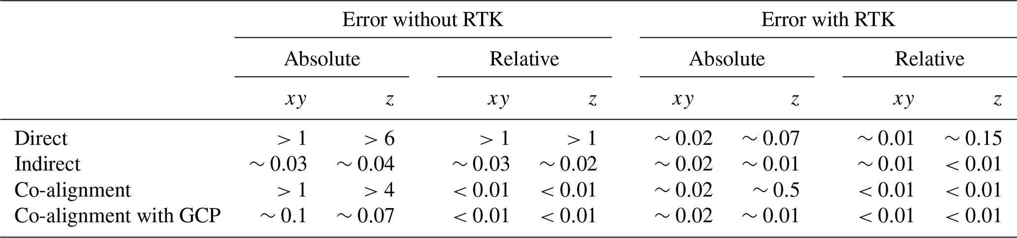
The consistently low mean relative errors (Table 1) of co-alignment underscore its usefulness for multi-temporal studies.

Automation, parameterization, and optimization of photogrammetry workflows were addressed by previous works: Śedź and Ewertowski (2022) investigated the fine-tuning of Agisoft Metashape parameters under the aspect of a singular flight with GCPs as a validation method. Tinkham and Swayze (2021) analyzed the influence of parameters, especially depth map filtering and alignment accuracy, on the ability to detect trees. They found that the highest quality increases the overall point count and no or mild filtering reproduces trees closest to reality. Blanch et al. (2021) have enhanced and automated co-alignment for fixed cameras in combination with GCPs. They state that their approach is not suitable for UAVs as it requires simultaneous photographs from the same locations. Hendrickx et al. (2018) examined the variation inherent in the proprietary algorithms of Agisoft Photoscan Professional, the predecessor of Metashape Professional. They concluded that the software can generate reproducible outputs with few variations, influenced by the quality settings. Variations are most pronounced in areas with low image overlap and complex terrain.

Agisoft Metashape Professional (Agisoft LLC, 2023b) alone is neither sufficiently convenient nor highly automatable for the co-alignment workflow, as it is designed as general-purpose photogrammetry software. Other software has been developed to streamline photogrammetry and alignment of PCs. The “Alignment Helper” by Jenkins and Johnson (2024) leverages Agisoft Metashape Professional, but it is designed primarily to enable rough manual alignment prior to automated co-registration. One such co-registration method is the widely used iterative closest point (ICP) algorithm (Besl and McKay, 1992). ICP is commonly used to align PCs (e.g., Jiang et al., 2021; Sevil et al., 2021) and is implemented in many open-source software solutions, such as CloudCompare (2024), but it requires a reasonable initial alignment estimate (Besl and McKay, 1992). Over et al. (2021) also automate Metashape workflows, but their scripts (Logan et al., 2022) do not implement the co-alignment workflow.

With the publication of Fully Automated Co-Alignment (FACA) we introduce a user-friendly, but powerful tool to apply co-alignment fast and reproducibly in a convenient framework. FACA represents the first dedicated software solution for the co-alignment workflow. Its applications can range from fine-tuning settings to a specific area of study, to applying co-alignment to multiple large areas with robust parameterization.

2 FACA

FACA is an open-source (GNU General Public License v3) application to automate the co-alignment workflow on a multi-temporal dataset as introduced by Cook and Dietze (2019).

2.1 Development motivation

We developed FACA to accelerate the application of the well-established co-alignment method, enabling streamlined deployment at any location with evolving temporal data, minimal preparation, and high adaptability and scalability. The software enhances both the efficiency and extendability of the co-alignment approach. Our initial goal for FACA was to support our research on the Baltic Sea coast, where we investigate mass movement potentials along cliffs in pilot regions, and aim to transfer this knowledge to other areas (Torizin et al., 2024; Schüßler et al., 2023). Data collected during the multiple field campaigns required rapid analysis, interpretation, and dissemination to partners and decision-makers. Additionally, we sought a workflow that could easily be adapted to other coastal sections that was effectively applicable by non-photogrammetry experts. As a result, FACA emerged as a user-friendly software solution capable of producing reliable results quickly. Although initially developed for UAV imagery, FACA is suitable for aligning large datasets of images, regardless of scale or capture method, provided that adequate computing resources are available. The FACA code was written, commented, and licensed to allow for easy modification by other practitioners.

2.2 Co-alignment with FACA

FACA, like all variations of co-alignment, leverages computer vision algorithms that underlie photogrammetry software. These techniques (e.g., Lowe, 2004; Bay et al., 2006; Rublee et al., 2011) detect key points – distinctive, invariant locations in an image – and match them across all images. Szeliski (2022) outlines four stages in this mode of operation: detecting, describing, and matching or tracking key points. Tracking is an alternative to matching limited to likely key points, such as those in similar areas across images. In the case of Agisoft Metashape, a proprietary variant (Semyonov, 2011) of the broadly used SIFT algorithm (Lowe, 2004) is employed. Its default matching settings use a priori knowledge about image locations to preselect images for matching, along with other metadata information, e.g., camera parameters and light conditions. This differentiates the photogrammetry workflow from the core computer vision algorithms while enhancing performance and precision (Agisoft LLC, 2023a). Images from individual UAV surveys, or general field campaigns or sessions, are stored in camera groups; these are all stored in one unit, or “chunk” in Metashape. Camera groups allow for survey-specific camera parameter optimizations. Tie points are key points that the algorithm matches across two or more images, establishing spatial relationships when aligned. When tie points span images from different surveys they align these surveys together, the eponymous co-alignment. From this point, SfM algorithms then use these tie points to optimize camera position and orientation through bundle adjustment. Finally, tie points are employed in the 3D reconstruction process, generating a sparse point cloud which can be filtered and refined within the original chunk. Afterwards, the surveys are separated, creating individual chunks and discarding key points not matched with its images while preserving location information and camera group specific calibrations. These new sparse point clouds are then processed separately to generate final products such as point clouds in FACA’s case.

FACA introduces flexibility compared to the original co-alignment workflow described by Cook and Dietze (2019), offering several optional steps that users can choose while maintaining the same foundational process. For instance, prior to key point matching and alignment, FACA allows users to adjust the accuracy of image location data, which can enhance co-alignment performance in cases where camera location information is uncertain across different surveys. This and other differences stem from the configuration possibilities FACA offers, see Table 2. FACA also differentiates itself from previous co-alignment works by not requiring human intervention, a path forward that Cook and Dietze (2019) already discussed.

Table 2 FACA parameters and their possible values.

2.3 Requirements and usage

FACA uses the Python API (Agisoft LLC, 2023a) of Agisoft Metashape Professional version 2.1.0 (Agisoft LLC, 2023b) to automate the co-alignment workflow and is compatible with versions 2.0.0 and later. FACA only requires a Python 3 installation with the standard library, an installed Metashape Python 3 Module, and a licensed copy of Agisoft Metashape Professional.

Every co-alignment relevant parameter that can be modified in the Metashape interface can also be altered via the Python API (Agisoft LLC, 2023a). Metashape also provides the ability to process batches, created using its main interface. This batch process is not a fully-fledged replacement for the Python API. In comparison it lacks many features, e.g., modifying existing chunks and labeling objects, in addition to losing the flexibility provided by Python, e.g., a custom interface and to dynamically name outputs. With the Metashape Java API (Agisoft LLC, 2024), there exists a third option on par with the Python API. We use Python because of our familiarity with the language and its popularity for Metashape scripting.

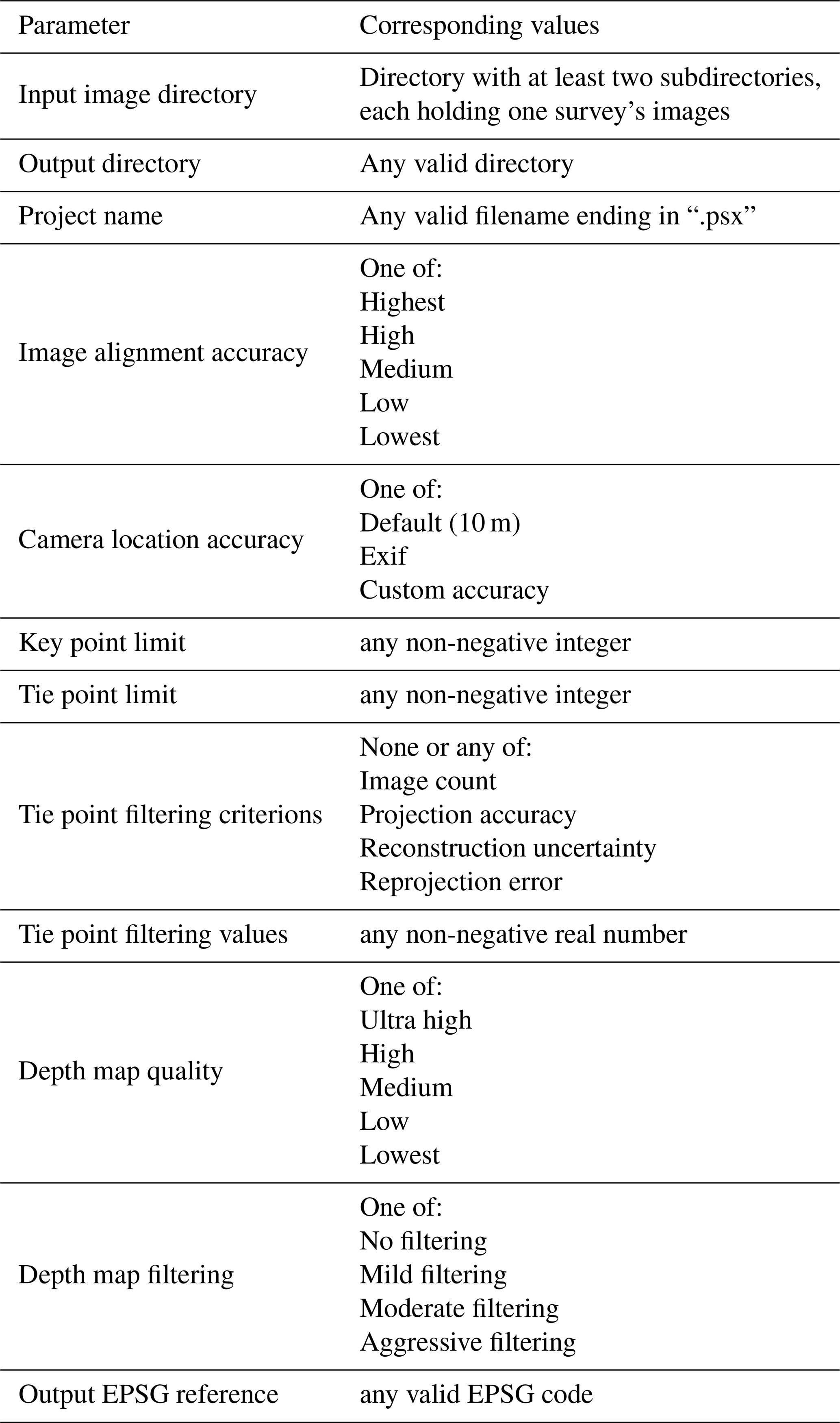
FACA imposes minimal rules on the input data and its structure, ensuring a smooth, automated workflow while maintaining adaptability for various use cases. The input directory must contain at least two subdirectories, each with one surveys images as .jpg files, allowing for any number of subdirectories as required by the user, without limiting the complexity or organization of the data hierarchy. All images must contain location information in their metadata. The name of the first level subdirectories will be used to reference the images they contain, as well as the outputs generated from those images. We found it convenient to name them based on their survey date.

FACA allows the use of predefined parameters, which are stored as sections within a configuration file. The default configuration file included with FACA contains a section that defines overarching parameters, such as the image input directory, output directory, and EPSG code for the output point clouds. These default values can be overridden by redefining them in other sections.

There are three ways to interact with FACA. The graphical user interface (GUI) (Fig. 1) uses the tkinter package and is the most accessible, but not as automatable as the alternatives. The interactive mode, where the software asks for each parameter, while providing the defaults as a suggestion and fallback. And, the script mode, where the user defines a configuration file and a section therein that FACA uses for the calculation. The user can optionally define parameters that differ from those specified in the configuration file section, for example, to apply established settings to an area with a different EPSG code or to modify input or output directories. If neither a configuration file nor a section is provided, but at least one calculation parameter is specified, the interactive mode will start, omitting prompts for the provided parameters. If all calculation parameters are provided as arguments, the calculation will start exactly as in script mode. Script mode allows FACA to be part of a larger automated workflow, e.g., applying filtering or color correction on the input images or removing vegetation and calculating statistics on the output PC. The modifiable configuration allows users to easily apply proven co-alignment workflows on their data, as well as find ideal workflows for their study areas with a sensitivity analysis. Configuration files can be created and modified manually or with the help of the GUI. For any other available setting, FACA uses the Agisoft default values, as specified in Agisoft LLC (2023a).

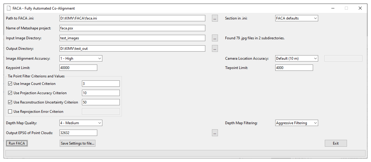
Figure 1 The FACA GUI allows the user to load, edit, and save parameters and apply co-alignment.

FACA records its steps and interim results, e.g., the number of detected surveys, corresponding images and tie point counts, the Metashape version used, and calculation parameters, in a time-stamped log file within the output directory. These small text files can be easily shared with peers to facilitate reproducibility, enhance workflow transparency, monitor performance, and assist in identifying and troubleshooting errors or issues. Additionally, the logs can be automatically parsed to generate figures for publications or to facilitate the automatic comparison of different parameterizations (Schüßler, 2024).

2.4 Parameterization

Parameters and possible values supported by FACA are listed in Table 2. Our streamlined approach allows us to quickly apply multiple co-alignment workflows discussed by other authors and examine their general transferability to other areas. FACA ships with multiple co-alignment parameters used previously in addition to its own defaults ready for use as part of its initial configuration file (Cook and Dietze, 2019; Nota et al., 2022; Saponaro et al., 2021; de Haas et al., 2021; Harkema et al., 2023; Omidiji et al., 2023; Moran et al., 2023). FACA emulates the parameters of these co-alignment approaches as far as they do not require additional manual inputs from the user and do not use depreciated features of Agisoft Metashape.

FACA users can choose any settings they want, either from a modifiable list based on previous works or by selecting their own. FACA default parameters emphasize practical automated applications of co-alignment. Because of this, they are conservative, especially the tie point filtering, as manual fine-tuning is not expected. We see these parameters as reasonable suggestions and invite practitioners to expand upon them for their needs.

The Image Alignment Accuracy setting controls the level of image scaling applied during camera position estimation (Agisoft LLC, 2023b). Undersampling (Medium, Low, and Lowest Image Alignment Accuracy) the images normally offers faster processing at the cost of detail and accuracy. Oversampling uses more detailed images to provide precise results, but does so at the cost of roughly twice the computing time compared the unmodified images. Using the original image resolution (High Image Alignment Accuracy) is a reasonable compromise.

Camera accuracy defines the expected positional accuracy of each camera's coordinates (Agisoft LLC, 2023b). The default of 10 m maintains some flexibility when using tie point matching with posterior knowledge from image metadata. This is crucial, as the accuracy of image location data can vary between UAV flights, often exhibiting different systematic offsets across sessions.

Key points are significant features detected in an image and tie points are key points matched across images; their limits define the maximal amount of each to consider during processing (Agisoft LLC, 2023b). High or no key- and tie point limits can introduce noise into the sparse point cloud and increase processing time, while low values can lead to missing features. We use the default values of 40 000 key points and 4000 tie points per image (Agisoft LLC, 2023a), because we found larger values take more time to process with no noticeable quality differences.

Rule-based tie point filtering can automatically identify and remove inaccurate or erroneous points, thereby reducing noise, optimizing following bundle adjustments, and improving processing efficiency while enhancing the overall precision in the final product (Agisoft LLC, 2023b). Agisoft Metashape Professional offers four built-in tie point filtering criteria: “Image count” filters tie points based on the amount of image in which they are visible and “Reprojection error” uses the maximum difference between measured and parameter adjusted coordinates of a tie point, normalized by the scale used. “Reconstruction uncertainty” uses the ratio of the largest to the smallest semi-axis of the error ellipse of tie points. “Projection accuracy” uses the average image scale used when getting the tie point projection coordinates divided by the number of images containing the tie point. We filter tie points that are not visible in at least three images, have a reconstruction uncertainty over 50, and projection accuracy over 10.

A depth map is generated for each image, representing the relative distances of objects from the camera's viewpoint (Agisoft LLC, 2023b). The depth map quality settings defines its resolution, and thus the detail and accuracy of the output geometry. “Ultra high” quality uses the images original resolution and each quality step quartering its pixel count, all the way to 1/256 at lowest depth map quality. We found the medium quality (1/16 resolution) to be suitable for use with UAV imagery.

Filtering the depth map removes tie point outliers, and can reduce noise in the output, but smaller details can be lost. In their documentation, Agisoft suggests “Aggressive” for drone images (Agisoft LLC, 2023b), which is why we employ this setting.

2.5 Technical workflow

Figure 2 shows the processing steps applied when running FACA with n different sessions. Every calculation expects all images taken during a flight session inside a directory, which, in turn, reside in a common main directory. The lower part of Fig. 2, below 'Copy Chunk n times', is simplified to show only one individual session i, but is applicable for all i from 1 to n.

Figure 2 FACA workflow. Dashed nodes indicate optional steps.

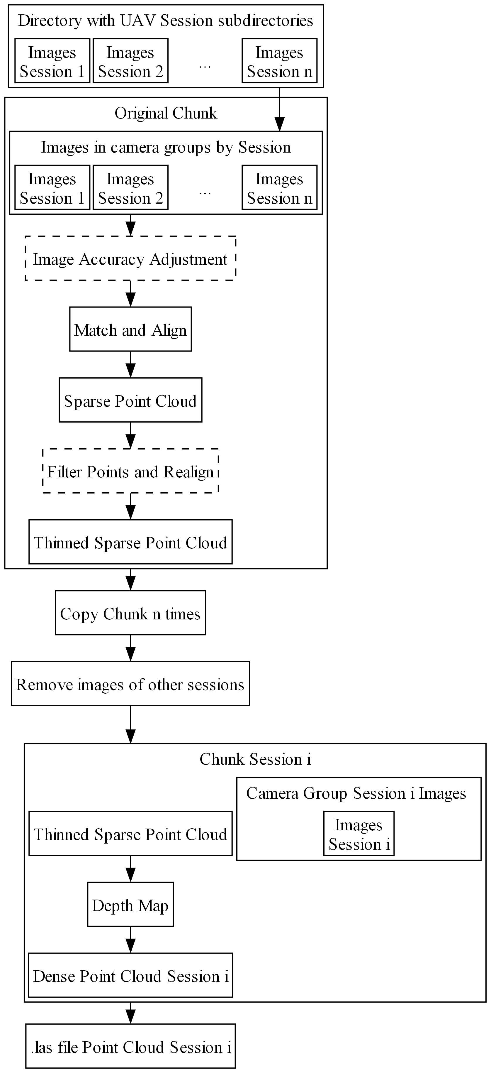
All images are loaded into the original chunk, where each session is organized within its own camera group, to facilitate individual camera parameter optimization. Each camera group is named according to its survey's subdirectory. Subsequently the image location accuracy can be optionally adjusted. Options include using the default value of 10 m in each direction (longitude, latitude, height), setting individual values for each direction, or utilizing precise measurements, e.g., from RTK equipment, if available. Following this, all images get matched based on the specified alignment accuracy, key point limit, and tie point limit. This step aligns all pictures to generate an initial sparse point cloud. The sparse point cloud can then be optionally thinned using any combination of tie point filtering criteria available in Metashape, while optimizing the alignment. FACA creates a separate copy of the original chunk for each flight survey, removing other session images. Thus, each chunk contains only the images from the respective session, organized within a single camera group, and a thinned sparse point cloud that only contains tie points visible in that survey. FACA then generates a depth map from these tie points with the specified quality and filtering mode. This depth map is used to construct a dense point cloud. The dense point cloud is subsequently exported as a .las file in the coordinate system defined by an EPSG code. The name of the final PC output is derived from the original subdirectory name of the session images.

3 Example application

To evaluate its real-world applicability, we use FACA to implement multiple co-alignment workflows in two coastal cliff erosion scenarios along Germany's Baltic Sea coast.

3.1 Study areas

We applied co-alignment with FACA in two study areas along Germany's Baltic Sea coast, see Fig. 3 and Table 3. The Sellin study area is located northeast of the town, along the western coastline of Rügen island. Its cliff consists of thick glacial–fluvial to glacial–limnic sands covering small amounts of till at the foot (Schulz, 1986). The bare, sandy plateau at the cliff top in the northern quarter contrasts with dense trees in the south. The study area spans approximately 600 meters of coastline, from coastal kilometer R089.030 to R089.630 (Staatliches Amt für Landwirtschaft und Umwelt Mittleres Mecklenburg, 2010).

Figure 3 Study areas overview. (a) Location of Mecklenburg-Western Pomerania in Germany; (b) location of the study areas in Mecklenburg-Western Pomerania; (c) northern part of the Sellin study area (29 February 2024); (d) southern part of the Sellin study area (29 February 2024); (e) central part of the Wustrow study area (18 October 2023); (f) bunker in the Wustrow study area pre-failure (16 March 2022); (g) the bunker post-failure (28 February 2024).

Table 3 Field campaign overview. Empty cells indicate the study area was not surveyed in this field campaign.

^* Four separate flight missions: 10 526, 12 662, 21 815, 18 117 m².

The Wustrow study area lies west of Niehagen and Althagen on Fischland, along the western coastline. It is a cliff consisting predominantly of till, partly overlain by eolian sand and cliff-edge dunes (Schulz, 1985). Landwards there is sparse forest in the southern quarter and agriculture in the north. The coastal retreat is progressing very quickly here due to wind exposure, wave erosion, weak silt material, and its shoreline parallel joint direction (Jacke and Lampe, 2010; Katzung, 2004; Schulz, 1985). North and south of the study area exist coastal protection structures, e.g., groins and breakwaters (Weiss et al., 1983; Bencard, 1998). Attempts to stabilize the coast line in the study area failed in the past (Bencard, 1998). The study area extends over about 1750 m of coastline, from coastal kilometer F177.350 to F179.100. (Staatliches Amt für Landwirtschaft und Umwelt Mittleres Mecklenburg, 2010).

Both study areas experience natural coastal erosion and are affected by landslides, leading to rapid changes in the cliff faces with minimal changes inland.

3.2 Data acquisition

We used a DJI Phantom 4 RTK in Terrain Awareness Mode (TAM). The drone is equipped with a 1^′′ CMOS 20 MP image sensor. RTK was enabled for all surveys. We took Nadir and oblique (45°) images along the same flight route. We combined the official German digital terrain model with 5 m resolution (DGM5) with the German Combined QuasiGeoid 2011 (GCG2011) to program the missions. TAM allows consistent ground sampling distance (1.1 cm per pixel at 40 m above ground for Nadir images) and image overlap. The automated flight plans were created using the DJI GS RTK App that came with the UAV remote controller. We planned for 70 % vertical and 80 % horizontal overlap of these images. Table 3 shows information concerning the eight field campaigns. Throughout most sessions, we supplemented the automatic pictures with ones taken manually. The were not primarily taken for Co-alignment, but for documentation purposes and to support other research areas in an overarching project (Schüßler et al., 2024b). Decisions to capture additional images were based on identifying significant changes in the cliff that warranted further documentation, as well as the availability of time in our project schedule and suitable weather conditions for UAV operation. The flight time is taken from the metadata of the first and last image taken in the area during that field campaign. In the first field campaign we only flew the southernmost automatic flight mission in Wustrow (10 526 m²). Before Field Campaign 6, in October 2023, we received a second Phantom 4 RTK – allowing us to fly parallel sessions. This speeds up the survey time and can reduce lighting differences between photos of the same survey. Starting with Field Campaign 7 in November 2023, we supplemented our automated flights with manual RGB flights conducted using a DJI Mavic 3M. However, we utilized images from these manual flights exclusively for generating point clouds in the Wustrow bunker area, due to the complex structure following the bunker's topple. Images of Field Campaign 7 present an additional challenge for our workflow as the ground is covered by snow. Because of this we did not examine Sellin but chose to survey Wustrow, as its steeper cliffs remained exposed.

After each field campaign, we reviewed the images and compiled a list of unsatisfactory photos, e.g., poor focus, drone parts or only sea visible. We excluded these from further processing.

3.3 Analysis

Our analysis focuses on the multi-temporal local precision and not the model's global accuracy. We analyzed the local precision of our results in two ways: firstly in an area without noticeable changes and secondly in areas with significant changes. For our stable area we used a 60.5 m² section of a rooftop unaffected by coastal erosion in the Sellin study area (54.3794° N, 13.7023° E). While the roof is in the border area (Fig. 4) it is the only sufficiently sized stable and flat area in the study area. In the stable area, we measured the cloud-to-cloud (C2C) distance of the PCs in the z (height) dimension compared to the first survey. C2C was selected for its parameter-free nature. Its use was further justified by the high and uniform point density of the relatively flat roof, despite its location near the edge, and the focus on vertical differences. The roof's location at the edge of the study area could lead to slightly exaggerated C2C distances, as the image coverage is not ideal compared to the center. We estimated the model's uncertainty with the range of distances in stable areas across surveys. Those with the lowest differences are considered best. There are no suitable anthropogenic structures in the Wustrow study area, thus we did not measure unaffected areas there. Table 4 contains the area with noticeable changes. The best models would accurately represent the changes we saw in the field in high detail. The coastal retreat should be recognizable over several flights, without outliers that reverse the trend.

Table 4 Areas with noticeable changes.

Besides these quality factors, we also measured the processing time, taken from the FACA log-file. We performed every calculation on the same workstation (CPU: Intel Xeon E-2286G; RAM: 128 GB DDR4 (2667 MHz); GPU: 16 GB Nvidia RTX 5000; HDD: HGST HUS726T4TALE6L4; OS: Microsoft Windows 10 Enterprise 22H2). The computation times should be regarded as relative references, not absolutes, as they can vary significantly depending on the available computing resources.

Figure 4 shows the location of the stable area (pink filled polygon in Fig. 4a), the area used to analyze changes in Sellin (green polygon in Fig. 4a), and the minimum bounding box of the images used to analyze the changes around the bunker (blue polygon in Fig. 4b) as well as the one used to quantify the coastal retreat (red polygon in Fig. 4b). The yellow polygons indicate the minimum bounding box of the automatic images taken during this field campaign. The stable area in Sellin lies just outside the minimum bounding box of images taken during automatic flight. The unstable areas in Wustrow (bunker in the south, coastal erosion in the north) are well covered by automatic flight images.

Figure 4 Orthophotos based on images from Field Campaign 6 with stable feature (pink filled polygon), sand cliff (green polygon), bunker area (blue polygon), coastal erosion area (red polygon), and the minimum bounding box (yellow polygons) of all images taken automatically on that day. (a) Sellin; (b) Wustrow.

The bunker serves us to visually identify and describe coastal erosion processes, especially after its collapse on 18 February 2024 (between Field Campaigns 7 and 8).

We used subsets of the Wustrow pictures to analyze the bunker and coastal erosion areas, see Table 5. Both datasets are freely available under the CC-BY-SA 4.0 license (Schüßler et al., 2024a, 2025a). They are the images that were taken within the defined bounding boxes (blue and red polygon in Fig. 4b) of the unstable areas.

Table 5 Number of usable images for the detail calculations of unstable areas in the Wustrow study area.

We quantified the coastal erosion in Wustrow by tracing the cliff top in the area of interest (see red polygon in Fig. 4b) with CloudCompare (2024) using the generated dense point clouds to create polylines. Then we exported them as Shapefiles and proceeded in QGIS (QGIS Development Team, 2024). In the geographic information system, we generated a line grid with the extent set to be slightly larger than the traced cliff tops, 1 m horizontal and 200 m vertical spacing. We discarded all vertical lines and rotated the horizontal ones 20° clockwise, so they are perpendicular to the coastline. Finally, we split the rotated features with two cliff tops and removed the parts outside of this region. Doing this resulted in roughly 380 measurements of coastal erosion per parameterization. Knowing the days between the UAV surveys, we interpolated the yearly coastal erosion. We used the same rotated line grid for all measurements.

We analyzed the changes in the Sellin cliff by clipping the area of interest (green polygon in Fig. 4a) out of the remaining dense point cloud. The underlying Sellin image dataset (CC-BY-SA 4.0 license) is available (Schüßler et al., 2025b). In this area, we calculated the M3C2 distance (Lague et al., 2013) for each pair of sequential surveys. We used M3C2 here because it is robust and allows us to measure the direction of changes. C2C was deemed unsuitable here, because it does not account for surface orientation and provides only unsigned distance measures. We always used the older of the two compared PCs as the basis for sub-sampling to generate core points with 0.25 m spacing. We configured M3C2 to use multi-scale normals between 0.5 and 4.5 m with 1 m step size and a projection diameter of 0.5 m. The clipping and M3C2 calculation were done with CloudCompare (2024).

FACA automatically logs the timestamps when generating a model. We used these logs to calculate time expenditures and compared them. The best model would both generate quickly and offer good local precision.

For an overview of parameters used in this example application of FACA see Table 6. We chose the parameters discussed in these works because of their range of values and good documentation in their respective articles. This work does not aim to evaluate the results of these previous studies but wants to show the capabilities of FACA across a wide range of parameters.

de Haas et al. (2021)Cook and Dietze (2019)

Table 6 Co-alignment parameters used, with their respective publication.

^* Adjusting the elevation by matching it with the known values from the launch points was not replicated here.

3.4 Results

3.4.1 Point cloud generation and filtering

Tables 7 and 8 show the tie point counts for the initial and tie point and dense point counts of individual survey chunks. The difference between “Original” and “Original – filtered” are tie points removed with filtering methods. There are 153 to 979 remaining tie points per image for a survey. The progression of tie point counts is shown in Figs. 5 and 6. These figures illustrate the number of tie points removed by each filtering method. For example, the “Image Count” criterion, represented by blue bars in both figures, indicates the number of tie points excluded for failing to meet the requirement of appearing in at least three images.

Figure 5 Sellin – distribution of total tie points for (a) de Haas et al. (2021) parameters, (b) Cook and Dietze (2019) parameters, and (c) FACA default parameters. Tie points filtered by different criterions are indicated by color: image count (blue), reconstruction uncertainty (orange), projection accuracy (red), and reprojection error (pink). Green bars indicate the number of tie points retained after filtering.

Figure 6 Wustrow – distribution of total tie points for (a) de Haas et al. (2021) parameters; (b) Cook and Dietze (2019) parameters; (c) FACA default parameters. Tie points filtered by different criterions are indicated by color: image count (blue), reconstruction uncertainty (orange), projection accuracy (red), and reprojection error (pink). Green bars indicate the number of tie points retained after filtering.

de Haas et al. (2021)Cook and Dietze (2019)

Table 7 Sellin – tie point (TP) and dense point (DP) counts. Tie points rounded to the nearest thousand and dense points to the nearest million.

de Haas et al. (2021)Cook and Dietze (2019)

Table 8 Wustrow – tie point (TP) and dense point (DP) counts. Tie points rounded to the nearest thousand and dense points to the nearest million.

de Haas et al. (2021)Cook and Dietze (2019)

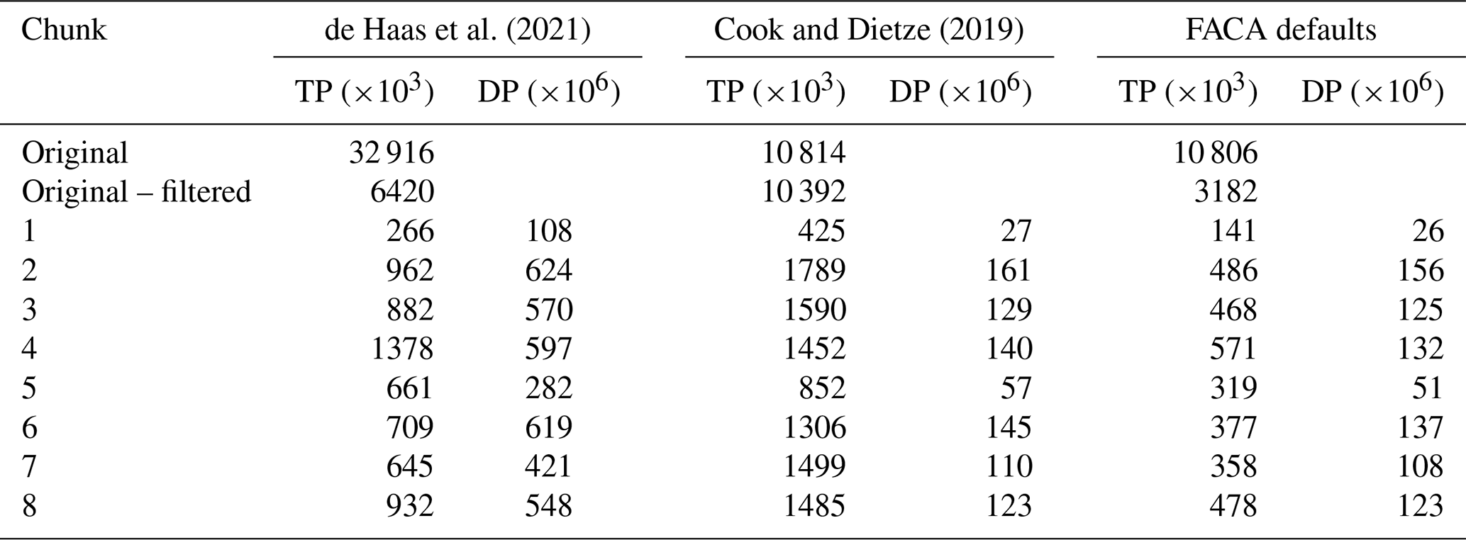
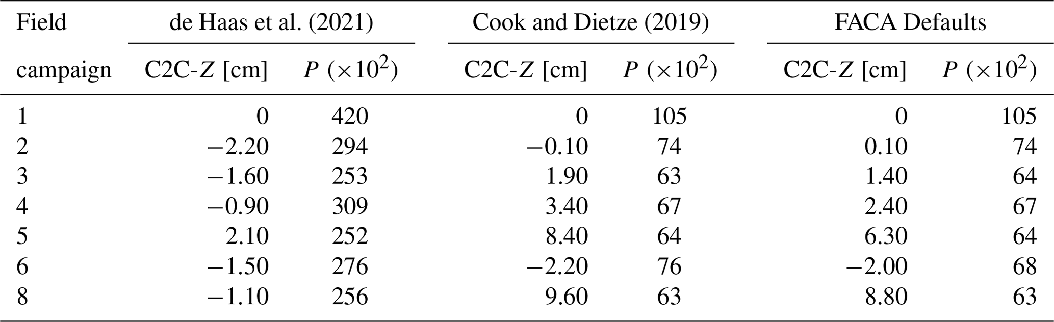
Table 9 Sellin stable area median cloud-to-cloud distances in the z dimension (C2C-Z), compared to Field Campaign 1, and dense point count (P). P rounded to the nearest hundred.

3.4.2 Stable area

Table 9 lists the median cloud-to-cloud distance in the Z dimension (C2C-Z) between each survey and the initial automatic Field Campaign 1 measured inside the stable area (pink polygon in Fig. 4a) and the corresponding dense point count. The arithmetic mean of the values in Table 9, excluding Field Campaign 1, is −0.87 cm for de Haas et al. (2021), 3.5 cm for Cook and Dietze (2019), and 2.8 cm for FACA defaults. Figure 7 displays violin plots of the C2C-Z between Field Campaign 1 and each subsequent campaign. The lines at the end show extrema, while the one in the middle signifies the median value, as listed in Table 9. The range of median distances are 4.3 cm for de Haas et al. (2021), 11.8 cm for Cook and Dietze (2019), and 10.8 cm for FACA default parameters.

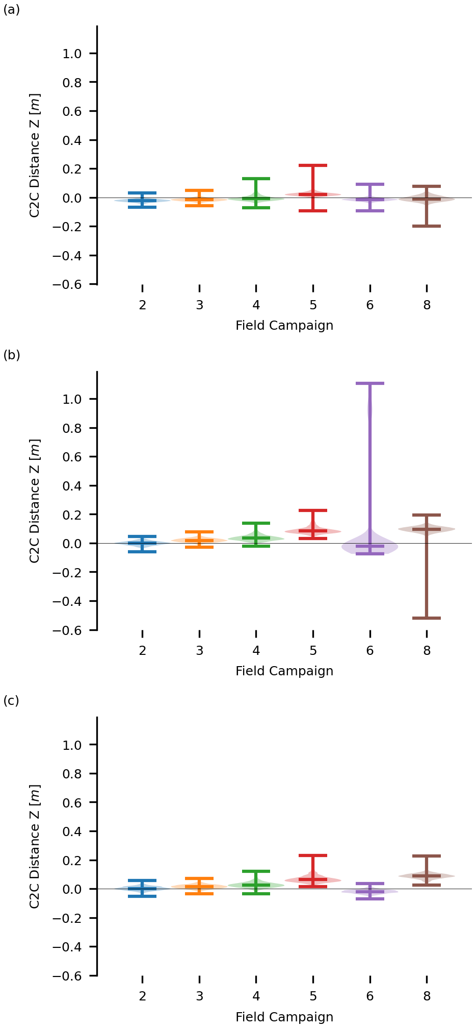
Figure 7 Sellin stable area violin plots of the cloud-to-cloud distances (Z dimension) with Field Campaign 1 as reference. (a) de Haas et al. (2021) parameters; (b) Cook and Dietze (2019) parameters; (c) FACA default parameters.

3.4.3 Unstable areas

Figure 8 contains point clouds of the sand cliff for each of the surveys flown in Sellin generated with FACA default parameters, clipped to the green polygon in Fig. 4a. Figure 9 displays the changes between subsequent field campaigns in the Sellin sand cliff as M3C2 distance point clouds. Figure 10 shows traced cliff tops in Wustrow for Field Campaigns 2 to 8. Statistics quantifying the interpolated yearly coastal erosion between Field Campaign 2 (16 May 2022) and both Field Campaign 7 (29 November 2023) as well as Field Campaign 2 and Field Campaign 8 (28 February 2024) are listed in Table 10. Figure 11 contains point clouds of the bunker area (blue polygon in Fig. 4b) in the Wustrow study area for each survey generated with FACA default parameters.

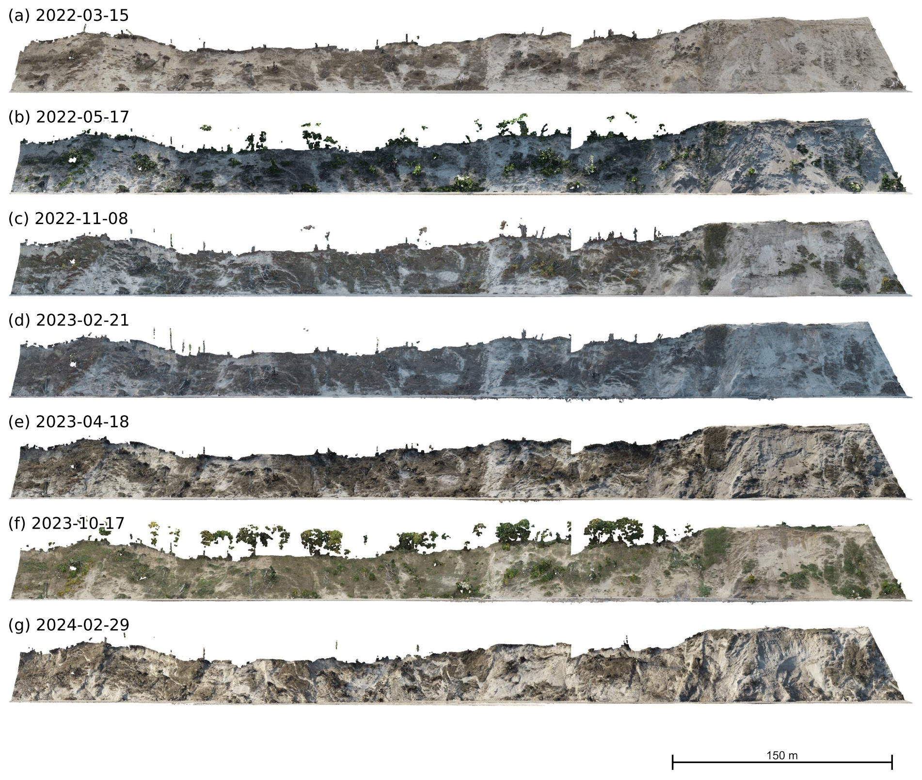
Figure 8 Dense point clouds showing the cliff in the Sellin study area of Field Campaigns 1 to 6 and 8 from the northeast based on FACA default parameters.

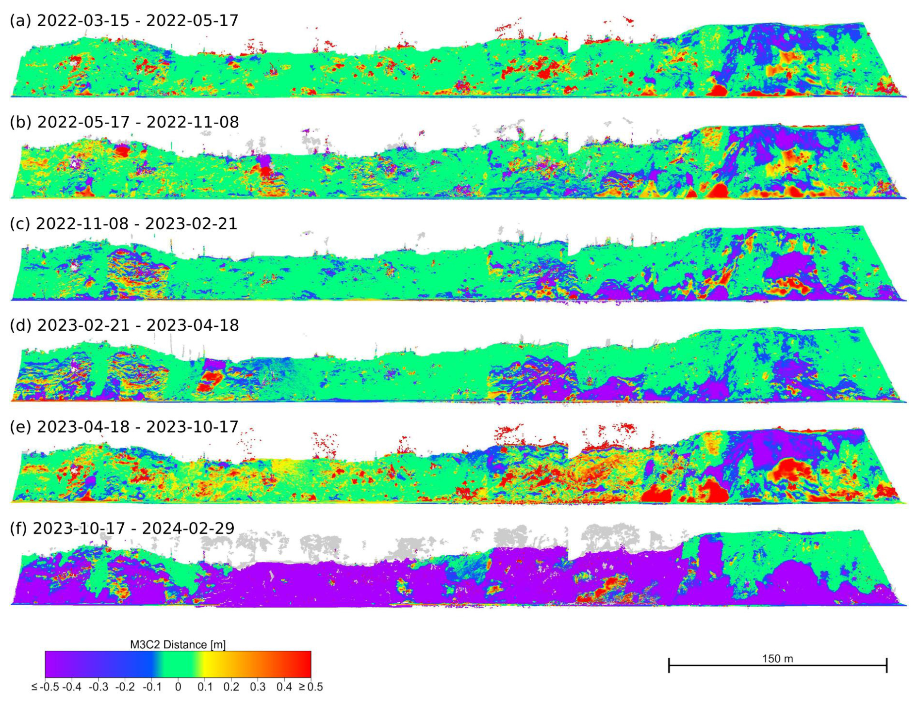
Figure 9 Dense point clouds showing the M3C2 distance calculated based on FACA default parameters of the cliff in the Sellin study area of Field Campaigns 1 to 6 and 8 from the northeast.

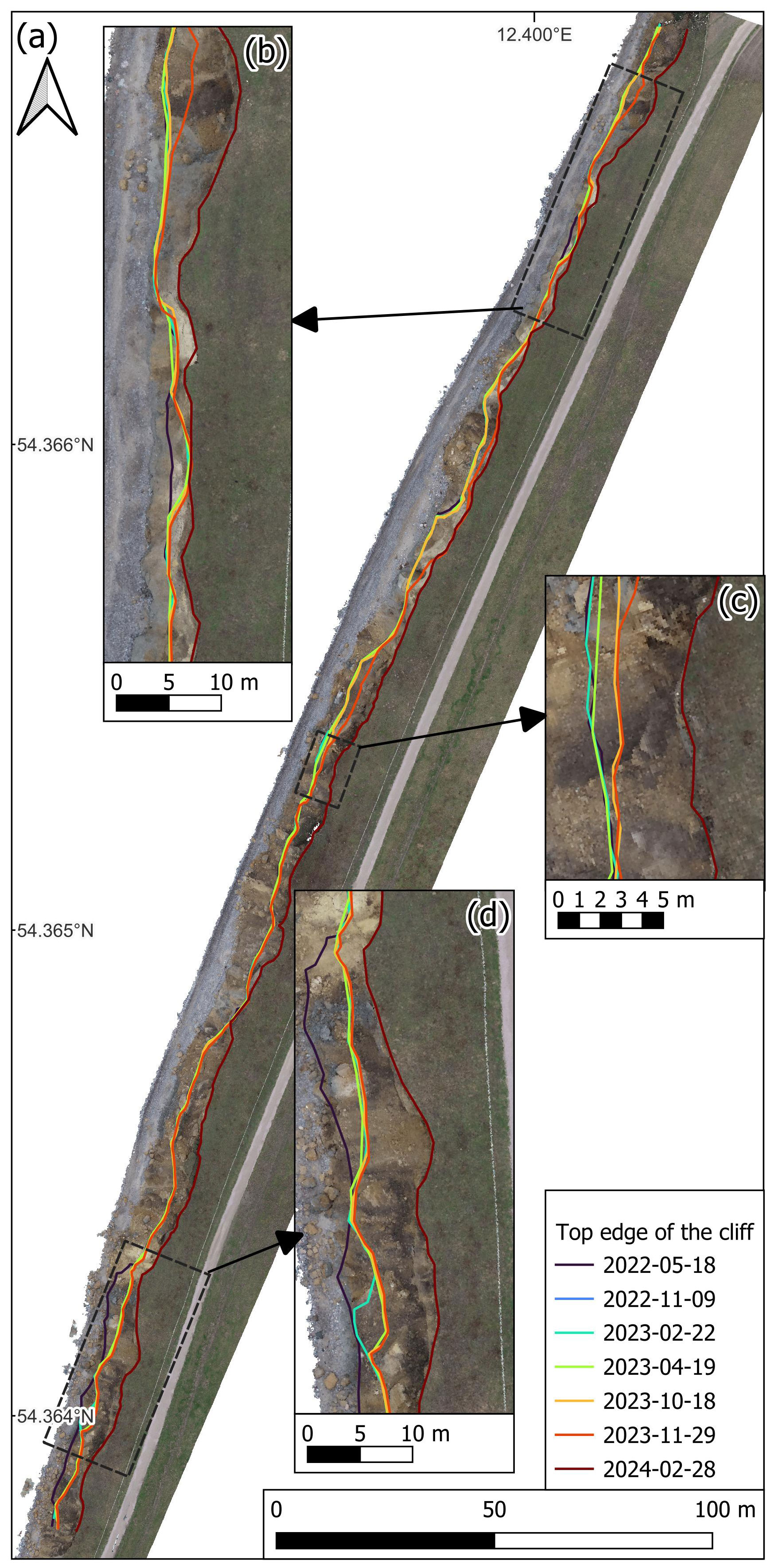
Figure 10 Cliff top development in Wustrow. (a) Top edge of the cliff from point clouds of Field Campaigns 2 to 8 with an orthophoto generated from the 28 February 2024 Flight with FACA default parameters; (b) northern detail; (c) center detail; and (d) southern detail.

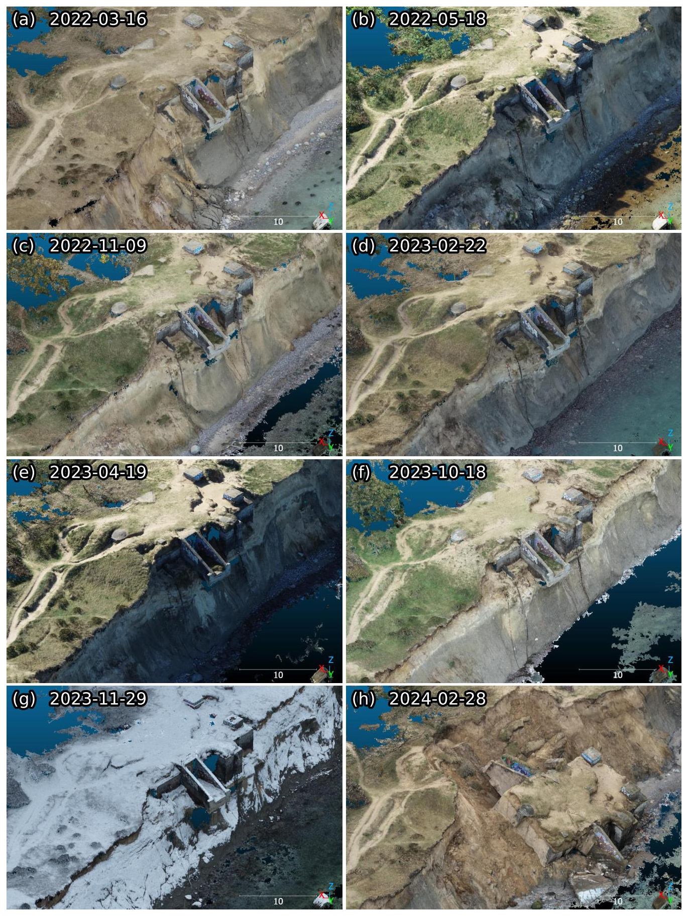
Figure 11 Point clouds of the bunker in the Wustrow study area from the northwest, generated with FACA default parameters for Field Campaigns 1 to 8.

de Haas et al. (2021)Cook and Dietze (2019)

Table 10 Wustrow – coastal erosion. Mean, median and standard deviation (σ) of interpolated yearly coastal retreat.

3.4.4 Computational resource efficiency

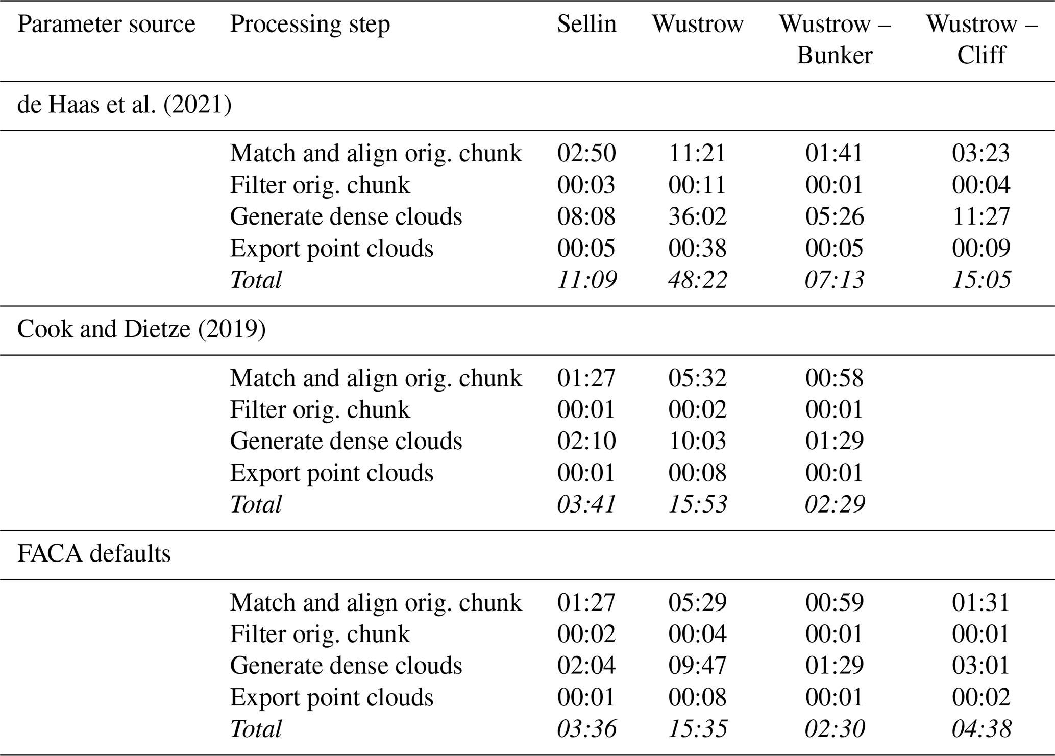
Table 11 lists the calculation time for each study area and co-alignment parameterization.

de Haas et al. (2021)Cook and Dietze (2019)

Table 11 Total and Selected Sub-step Time Expenditure in Hours:Minutes.

3.5 Discussion

3.5.1 Point cloud generation and filtering

The filtering methods were applied sequentially in the order listed in Table 2. This results in the first applied filter removing obvious points that most likely would have also been filtered by other methods, e.g., a tie point based on just two images is also likely to have a low projection accuracy. The reprojection error filter used with de Haas et al. (2021) parameters removes no points in both study areas because it is the last applied criterion and the tie points have been thoroughly thinned beforehand. Despite this, we consider the application of multiple filters useful, because they apply different quality criteria to the tie points and are not time-intensive. The threshold of each filter should ideally be based on the individual survey flown, but the differing surveys examined in this work show that generalizations are feasible. Given that the method of co-alignment is fundamentally based on finding tie points between multiple surveys, we consider the image count filter with a threshold ≥3 the most important one, especially given its easy-to-interpret nature.

The higher key point and tie point limits of the de Haas et al. (2021) parameters result in over three times the original tie points compared to the other two parameter combinations. The FACA default parameters generate the lowest tie point count after filtering. The Cook and Dietze (2019) parameterization starts with a comparable number of tie points, but they retain multiple times the de Haas et al. (2021) and FACA default ones after filtering.

The default conservative filters in FACA are designed to minimize noise, accepting the trade-off of a sparser point distribution, with the goal of enabling fully automated processing without human validation of each point cloud.

In addition to different filtering methods and changes in the landscape between field campaigns and or study areas, we interpret part of the fluctuation of tie points as a result of inefficient manual image capturing. This highlights the efficiency of well-planned automatic surveys to at least generate a general baseline to optionally expand upon.

3.5.2 Stable area

Stable areas between surveys are a prerequisite for the co-alignment workflow (Cook and Dietze, 2019).

The comparatively low global accuracy results in very slight shifts in the position of the polygon selected for comparison of the stable area between different co-alignment parameterizations, but it never shifts to unstable areas, i.e., off the roof.

Ideally, the median cloud-to-cloud height distance between survey 1 and subsequent surveys in stable areas is close to zero because there were no observable changes in the stable area during our field campaigns. We explain the differences with uncertainties in the creation of tie points, inaccurate camera location information, and the location of the stable area outside the main area covered by automatic flight routes among others.

The de Haas et al. (2021) parameters yielded the lowest overall median C2C distances in the height dimension. This outcome is influenced by the distance calculation method, nearest neighbor distance, which, when combined with the high point density of the de Haas et al. (2021) point clouds (approximately three to four times denser than those from the other two parameterizations, see Table 9), increases the likelihood of close correspondences in the global C2C analysis.

We did not use a local C2C model or the more advanced Multiscale Model to Model Cloud Comparison (M3C2) approach (Lague et al., 2013) here because they would ideally require specific settings for each output cloud, making comparisons more complex.

Choosing the point cloud of Field Campaign 1 as a reference is ideal because it is the densest one, thus minimizing the overall nearest neighbor distance, and it facilitates the interpretation of changes relative to initial values.

We interpret the range of values in the Sellin study area as a result of the flight height and location of the rooftop. The violin plots of Fig. 7 show that the C2C distance (Z dimension) distribution is similar for different parameterizations. We interpret outliers, e.g., Field Campaign 6 in Fig. 7b, as errors in the calculation of Agisoft Metashape.

Overall we show that there are suitable stable areas for co-alignment in the Sellin study area. Calculating the range of the median C2C distance (Z dimension) allows us to better interpret the uncertainties when examining the unstable cliff area in Sellin. While they are too small for a meaningful comparison between parameters, due to the aforementioned low global accuracy, there still exist stable objects in the Wustrow study area (e.g., benches, bins, and other smaller anthropogenic objects), underpinning our results.

3.5.3 Unstable areas – Sellin sand cliff

We decided to limit the difference calculation to the actual sand cliff, but decided against filtering out the thin vegetation therein as it is part of the moving landslide mass. Overall we observed more pronounced erosion in the northern quarter of the cliff because of the sparser vegetation in the cliff and at its top. Despite the far southern side being outside the bounding box of automated flights, see Fig. 4, there are no visible anomalies in the resulting point clouds (Fig. 8) and the M3C2 calculation (Fig. 9).

The first and second field campaigns (Fig. 8a and b) show little change (Fig. 9a), due to the small time delta (63 d), but the mutually reinforcing movements typical for the cliff are already visible: flows in the sand cliff face and slides at the foot of the cliff.

The slides occur as Baltic Sea abrasion removes material from the slope foot, steepening the slope, and triggering sand movement until it reaches its angle of repose (or steeper if stabilized by vegetation) and can be intensified by precipitation. Alternatively, once dried, the sand loses cohesion and becomes unstable, initiating flow.

Topples of vegetation bound material are visible in Fig. 9b, the difference between Fig. 8b and c. Figure 8c and d, and their difference Fig. 9c, shows a continuation of the general trends. The difference of Fig. 8d and e (Fig. 9d) shows flows continuing and new slides and flows in the southernmost area. When directly comparing Fig. 8e and f, they confirm that the flows persist, although it is not discernible in Fig. 9e due to vegetation growth, which impedes interpretation. Figure 8f and g show pronounced differences (Fig. 9f) in the cliff: two large (>10 m width) slides in the northern part, multiple toppled trees from the crown, and deeper seated slides in areas that previously exhibited flows.

These final changes reveal glacial till beneath the sand, which leads to the cliff steepening beyond the sand's angle of repose. Once the coastal erosion weakens the glacial till it could lead to larger single event landslides in that area.

3.5.4 Unstable areas – Wustrow coastal retreat

The Wustrow study area comprises multiple flight missions (Table 3) to maintain visual line of sight to the UAV. To cover the entire area, we operated from two different starting points and relocated the RTK base station between missions. As all images use the RTK base station as a reference, moving the base can introduce variations in the recorded image positions across flights conducted within the same field campaign. These inconsistencies can, in turn, challenge the proprietary and non-deterministic algorithms within Metashape, potentially leading to alignment errors currently not handled by FACA. To mitigate these issues, we did not use the PCs generated for the whole Wustrow study area using de Haas et al. (2021) and FACA Default parameters. Instead, we generated new, smaller PCs covering only single flight missions to analyze coastal erosion while employing the same parameters.

The values in Table 10 were interpolated based on the cliff top's position in the second, seventh, and eighth field campaigns, as the first survey did not cover this area. The inherent uncertainties when tracing the cliff top by hand are the likely explanation for the variation between yearly coastal retreat values for different co-alignment parameterizations. All generated PCs were sufficiently dense and detailed to allow accurate tracing of the cliff crown, with insignificant uncertainty regarding its location.

The difference in cliff top measurements in the seventh and eighth field campaigns in Fig. 10a indicate that the erosion process is highly inconsistent, likely driven by the significant impact of storm surges and severe weather events. Figure 10b–d further demonstrates that the retreat is not uniform along the coastal cliff, with retreat occurring more rapidly in zones of weakness, eventually isolating and eroding more stable areas.

Overall, the measured coastal retreat between surveys two and seven is consistent with previous estimates for this area, which range from 0.8 to 1.4 m a⁻¹ as collected by Schulz (1985) and from 0.38 to 1.09 m a⁻¹ by Ullrich (1983). The calculations by Hoffmann and Foy (2023) of 0.65 m a⁻¹ (1835–2021) and 0.74 m a⁻¹ (2005–2021) are both close to, but slightly lower than, our results. We attribute the over 2.3 m a⁻¹ coastal decline we measured between surveys two and eight to the impact of a recent storm surge and the relatively short time span of just under two years.

Additional drone surveys could provide more data and reveal a clearer trend. This would be particularly valuable as older documents and maps, such as those from the 19th century which are currently used for long time difference calculations (Hoffmann and Foy, 2023; Schulz, 1985), are often hard to georeference, leading to significant uncertainties. New data would also be valuable for investigating and monitoring the assumed impacts of climate change (Meier et al., 2022).

3.5.5 Unstable areas – Wustrow bunker

The progress of coastal erosion in the southern part of the Wustrow study area is visualized in Fig. 11. The pictured bunker is located approximately 350 m beyond the southern end of the traced cliff top (Fig. 10), see Fig. 4b.

The partially intact vegetation on loose material at the bottom of Fig. 11a indicates that there has been a recent landslide. North of it another slide occurred between Fig. 11a and b. We interpret it as the result of abrasion at the toe of the slope and of loose landslide debris by the Baltic Sea and thus its steepening in combination with a loss of cohesion inside the material and change of geometry due to the older landslide at its edge. Figure 11c and d shows the removal of further landslide debris, revealing a boulder that is heavy enough to defy tidal forces. Figure 11d first shows the coastline retreating far enough along the borders of the bunker to reveal its northern wall. With the removal of loose material from the landslide, underlying gray glacial till is revealed and a wave-cut notch begins to form (Fig. 11d). This wave-cut notch widens in Fig. 11e, while the aftermath of an earth fall or topple south of the bunker is visible. Over the summer of 2023, the erosion along the edge of the bunker moves further inland (Fig. 11e and f). Figure 11f shows the collapse of the slope above the wave-cut notch, the further movement of the cliff top at the sides of the bunker, and over-steepening of the cliff face. Between Fig. 11e, f, and g a steepening of the lower parts of the cliff is visible. These direct abrasion results appear most pronounced underneath the front of the bunker between Fig. 11f and g. The erosion below and at the sides of the bunker in combination with its high specific weight and inflexibility resulted in its topple, see Fig. 11h.

Throughout the time series in Fig. 11, the effects of precipitation-induced erosion are visible at the bunker walls facing the Baltic Sea, also highlighting the local luv–lee effect, where forces are diverted from the robust bunker into the susceptible material surrounding it. Given the high rates of coastal erosion in the area and the lack of coastal protection, it was only a question of time before the bunker toppled into the Baltic Sea. We perceive that there were signs of a potentially imminent bunker topple as early as November 2023. The erosion has progressed far enough underneath the bunker that the dense point cloud contains holes (Fig. 11g) pointing to very steep slope angles only possible due to the robust bunker. These circumstances, combined with a storm surge (Perlet-Markus, 2023), resulted in the final toppling of the bunker (Fig. 11h). This event highlights the potential dangers posed by dynamic coastal processes and underscores the importance of using such occurrences to raise public awareness of natural hazards.

3.5.6 Computational resource efficiency

The values in Table 11 align with our expectations. Because Cook and Dietze (2019) and the FACA defaults use the same parameters for matching and aligning of the original chunk they take nearly the same time in each area for this step.

Compared to the total time taken to apply the workflow, the time expenditure to filter the tie points is negligible, yet we still see differences based on the tie point count and the number of filtering methods applied. Time taken to filter out tie points might even accelerate the latter steps in the workflow because there are fewer points to consider when generating dense point clouds.

Dense cloud generation required similar processing times for both Cook and Dietze (2019) and the FACA default parameters, whereas de Haas et al. (2021) was approximately four times slower due to its higher key point limit and use of high-quality depth maps.

We noticed no significant quality differences in the final dense clouds. This is evident by the similar results across parameterizations in Table 10. Other researchers might benefit from the slightly lower uncertainties in stable areas, as shown in Fig. 7 and Table 9, and may consider the longer computation time an acceptable trade-off. The amount of unfiltered tie points scales nearly linearly with the matching alignment time.

It takes roughly the same time to apply the whole workflow on every study area with both Cook and Dietze (2019) and FACA defaults as it takes to just apply the workflow in Wustrow with de Haas et al. (2021) parameters. This shows the substantial impact of parameter choice on computational and time requirements.

4 Conclusions and outlook

Co-alignment is a good technique to prepare point clouds for change detection and time series analysis. We showed that it provides good results even if the terrain has undergone extensive, study area-wide change, e.g., after snowfall, given enough alternative surveys to generate common tie points. Our comparative study of different co-alignment parameters shows that FACA is an excellent tool to easily generate reproducible research. We hope that the streamlined approach to co-alignment offered by FACA allows researchers to work around some of the method's drawbacks, i.e., the impact of time-consuming recalculations after new surveys can be lessened by the automation. The easy configuration allows practitioners to find suitable parameters for their study area. Detailed logging can grant insights into the workflow.

Moving the workflow beyond Metashape either as a stand-alone solution or to free software, e.g., OpenDroneMap Authors (2020), could be a next step. Doing so would significantly lower the financial barrier to entry, just as FACA lowers it for configuring and using co-alignment. The more open approach would also allow for co-alignment specific optimizations, that are usually not viable in default photogrammetry workflows, such as defining different quality criteria for tie points based on whether the images were taken during the same survey or not.

Modifying FACA to allow the usage of GCPs would further improve the software. By using computer vision, this task could potentially also be automated. Another interesting step forward would be to use a priori knowledge to designate or automatically detect (Peppa et al., 2018) stable areas to establish ground control areas, to minimize the noise in that area, and, thus, better align every part of the study area. This could be done on the stable subset with the iterative closest point algorithm and the other parts of the point cloud are then transformed to fit the registered stable areas. The custom software approach would also benefit this idea, as tie points in these areas could be treated differently from the ones in dynamic areas.

We hope that the methods introduced in this article help widen the adoption of UAVs for multi-temporal dataset generation, not only in the field of natural hazards but also in other parts of the applied geosciences, e.g., geotechnics, geomorphology, and opencast mining.

We publish our code as open-source software not only to encourage its use but also to allow others to examine its underlying mechanisms, contribute their ideas, and foster discussion among users.