the Creative Commons Attribution 4.0 License.
the Creative Commons Attribution 4.0 License.
 | 09 Sep 2025
ROCKE-3D 2.0: an updated general circulation model for simulating the climates of rocky planets
Kostas Tsigaridis
Andrew S. Ackerman
Igor Aleinov
Mark A. Chandler
Thomas L. Clune
Christopher M. Colose
Anthony D. Del Genio
Maxwell Kelley
Nancy Y. Kiang
Anthony Leboissetier
Jan P. Perlwitz
Reto A. Ruedy
Gary L. Russell
Linda E. Sohl
Michael J. Way
Eric T. Wolf
We present the second generation of ROCKE-3D (Resolving Orbital and Climate Keys of Earth and Extraterrestrial Environments with Dynamics), a generalized three-dimensional general circulation model (GCM) for use in Solar System and exoplanetary simulations of rocky planet climates. ROCKE-3D version 2.0 is a descendant of ModelE2.1, the flagship Earth system model of the NASA Goddard Institute for Space Studies (GISS) used in the most recent Intergovernmental Panel on Climate Change (IPCC) assessments. ROCKE-3D is a continuous effort to expand the capabilities of GISS ModelE to handle a broader range of planetary conditions, including different atmospheric planet sizes, gravities, pressures, and rotation rates; more diverse chemistry schemes and atmospheric compositions; diverse ocean and land distributions and topographies; and potential basic biosphere functions. In this release we present updated physics and many more supported configurations which can serve as starting points to simulate the atmospheres of rocky terrestrial planets of interest. Two different radiation schemes are supported, the GISS radiation, valid only for atmospheres similar to that of modern Earth, and SOCRATES, which is more generalized but more computationally expensive. While ROCKE-3D can simulate a very wide range of planetary and atmospheric configurations, we describe here a small subset of them, with the goal of demonstrating the structural capabilities, rather than the scientific breadth, of the model. Three different atmospheric composition options (preindustrial Earth, the aerosol-free and ozone-free atmosphere used in ROCKE-3D 1.0, and an anoxic atmosphere with no aerosols), three ocean configurations (prescribed, Q-flux, and dynamic), and two resolutions are described: the medium resolution (4×5° in latitude and longitude, previously used in ROCKE-3D 1.0) and the fine resolution, which has double the resolution in the atmosphere and 4 times the horizontal and 3 times the vertical resolution in the ocean. Finally, for the land surface hydrology, we have introduced generalized physics for arbitrary topography in the pooling and evaporation of water and river transport of water between grid cells, as well as for the vertical stratification of temperature in dynamic lakes. We quantify how the different component choices affect model results and discuss the strengths and limitations of using each component, together with how one can select which component to use. ROCKE-3D is publicly available, and tutorial sessions are available for the community, greatly facilitating its use by any interested group.
- Article
(11752 KB) - Full-text XML
- BibTeX
- EndNote


Three-dimensional general circulation models (GCMs) have been in existence for several decades, dating as far back as the 1950s (Phillips, 1956). Their use has mostly been in the climate modeling of modern Earth, as well as in more generic studies of atmospheric (e.g., Showman et al., 2013) and oceanic circulation (e.g., Bryan, 1969). Initially these models were focused on the atmospheric component and have been called atmospheric GCMs, or AGCMs (Manabe and Wetherald, 1967). The next major component to be added was the oceans, which provided a source of water to the atmosphere, and a variety of computationally efficient ocean models were coupled to the AGCMs and became known as AOGCMs (Manabe and Stouffer, 1993). These computationally efficient oceans included those with fixed sea surface temperatures (sst) and later what were termed Q-flux oceans where the heat (Q) fluxes (flux) between oceanic grid cells were fixed at model start (e.g., Russell et al., 1985; Slingo, 1982). Initially the fluxes used came from satellite observations or from numerical ocean models (e.g., Bryan, 1982; Miller et al., 1983). The depths of these oceans had no standard fixed values, but researchers have typically used depths up to ∼100 m. These computationally efficient types of oceans have a variety of names such as thermodynamic and slab, among others (see Way et al., 2017, for more details). In the past couple of decades the Earth GCM community has moved to fully dynamic oceans that explicitly calculate horizontal and vertical ocean heat transports at resolved spatial scales while also including a range of parameterized processes that operate on smaller unresolved scales, but they are more computationally expensive than the simpler sst or Q-flux oceans. In modern times the exoplanet community has started to use a parameterized ocean, but they typically use Q-flux type oceans where the fluxes are set to zero (highlighted as Q-flux = 0 here when relevant). This is because they have no way to set the ocean heat fluxes due to the lack of any observations and have typically been unwilling to use fully dynamic oceanic models (AOGCMs) to estimate the fluxes, due to the increased computational cost and additional free parameters, given the lack of information about oceans in exoplanets. This approach obviously has limitations in accurately modeling the climate, with perhaps the most “notorious” being the “eyeball” world of tidally locked planets around M-dwarf type stars (e.g., Pierrehumbert, 2010). For example, using the ROCKE-3D model Del Genio et al. (2019a) showed in simulations of Proxima Centauri b that large-scale circulation patterns (see their Figs. 1a, b and 2a, b) and mean surface temperatures (Q-flux=0 had a mean surface °C, while the dynamical ocean had °C) can differ drastically between a model using a Q-flux = 0 and a fully dynamic ocean model. Yet in other scenarios the differences can be minor as seen in the work of Way et al. (2018) in a parameter study of slowly rotating worlds with increasing insolation. They showed that Earth-like planets around solar-type stars showed large mean surface temperature differences when the length of day was similar to that of modern Earth, but at longer length of days and higher insolations the differences were marginal (<2 °C; see their Fig. 2). ROCKE-3D is capable of modeling the atmosphere coupled to any of the ocean models described above. ROCKE-3D also has fully coupled cryosphere and land surface models, interactive ocean biogeochemistry, and interactive atmospheric chemistry. Not only are these processes vital for a model Earth GCM, they are also important for studying the climates of exoplanets found at the inner and outer edges of the habitable zone (e.g., Kopparapu et al., 2013). Herein we discuss the second release of the ROCKE-3D GCM. Section 2 provides a detailed model description; Sect. 3 describes how ROCKE-3D evolved from its parent Earth GCM, ModelE; Sect. 4 presents model configurations than can be utilized by the end user; and Sect. 5 is the discussion.
ROCKE-3D version 1.0 (Way et al., 2017) was a descendant of GISS ModelE2, described and thoroughly evaluated by Schmidt et al. (2014). Since then, several bug fixes, updates, and upgrades to both ROCKE-3D and ModelE have happened in parallel and are brought together in ROCKE-3D version 2.0, which is described in this work. There are two development pathways that contributed to ROCKE-3D 2.0: the Earth-centric development in ModelE2.1 is summarized in Sect. 2.1, while the planetary-centric development in ROCKE-3D 2.0 is described in Sect. 2.2. More specifically, several physics changes were introduced in GISS ModelE2.1, which is the version of ModelE used in the Coupled Model Intercomparison Project phase 6 (CMIP6; Eyring et al., 2016), and are thoroughly described elsewhere (Kelley et al., 2020). Additional changes present in ModelE2.1 that are either bug fixes or structural enhancements since the CMIP6 version of the model were also ported to ROCKE-3D 2.0 and are briefly described in Sect. 2.1. These latter enhancements include major changes in the prognostic tracer code present in ROCKE-3D 2.0, which will be described elsewhere, since they are not used here. The planetary-related changes, which include both physics enhancements and diagnostics enrichment relevant to the generalized ROCKE-3D 2.0 model, are described in Sect. 2.2. Here we study the climatology simulated by the model using a fixed atmospheric composition per configuration, in the exact same way that was the case for ROCKE-3D 1.0 (Way et al., 2017).
The hydrostatic ModelE2.1 dynamical core employed in ROCKE-3D utilizes the Arakawa B grid staggering, whose benefits at coarse resolution over the conventional C grid were argued by Hansen et al. (1983); this reference provides other introductory details as well. Momentum and air mass transport continues to employ the Arakawa centered-differencing approach, with dissipation at small scales applied via a Shapiro filter. A prominent update from the Hansen et al. (1983) version is that potential temperature, humidity, and other scalars are transported using the conservative quadratic upstream scheme (QUS; Prather, 1986), whose implicit numerical diffusion is inherently very scale-selective. The benefits of the QUS for tracers were described in Rind and Lerner (1996). Air mass and momentum fields are advanced using a leapfrog scheme with a time step respecting the Courant–Friedrichs–Lewy (CFL) condition for the barotropic mode (Lamb wave), whose horizontal velocity is on the order of the speed of sound. Potential temperature advection is performed on the even leapfrog time steps, with temporal interpolation as needed for hydrostatic integrations. Since humidity and tracer fields do not directly affect the dynamics in this version, they are advected on a longer, but locally adaptive, time step, respecting local CFL conditions for wind speeds, which are typically much less than the speed of sound.
The ROCKE-3D atmosphere includes hydrostatic resolved dynamics and parameterized sub-grid vertical transport via turbulent eddies and vertically extensive cumulus-cloud convection; stratiform cloud fraction is diagnosed from relative humidity and convective cloud fraction from vertical mass exchange rates; condensation of water vapor is explicitly calculated in clouds as a source of precipitation and the liquid and ice hydrometeors seen by radiative transfer; optional chemical and aerosol tracer constituents propagate through all these phenomena as they undergo their own processes. The evolutions of these processes are outlined in a series of papers (Bauer et al., 2020; Kelley et al., 2020; Schmidt et al., 2006, 2014) which themselves may refer back to component-specific original version descriptions, e.g., Del Genio et al. (1996) for stratiform clouds or Lacis and Oinas (1991) for longwave radiative transfer.
Sea ice in ROCKE-3D 2.0 is treated as two mass layers, each containing two thermal layers: (1) the top mass layer has a fixed thickness of 0.1 m and contains both ice and snow (snow thickness evolves with precipitation) and (2) the bottom mass layer is ice only and can grow infinitely in thickness (with a minimum of 0.1 m). Sea ice thermodynamics are based on the brine pocket or “BP” formulation, with both mass and energy budget (Schmidt et al., 2004), and include brine rejection through gravity drainage and flushing of meltwater. Ice sheets are bottomless, but only the upper 3 m is used for thermodynamics computations. Those are represented by two layers of ice: 0.1 m at the top and 2.9 m at the bottom. The ice can accumulate a layer of snow on top of it. The snow in excess of 0.1 m of dense ice equivalent is converted to the ice and pushed down the ice layers. If iceberg calving is enabled (optional) the accumulated ice is distributed as icebergs to the ocean cells according to a prescribed mask (specified in an input file). The albedo of the ice sheet snow either is fixed at 0.8 (default for modern Earth) or is updated according to a snow aging algorithm as described in Hansen et al. (1983).
The vegetation model coupled to ROCKE-3D is the Ent Terrestrial Biosphere Model (Ent TBM). This dynamic global vegetation model (DGVM) provides simulation of biophysics (albedo, photosynthesis, transpiration, plant, and soil respiration) given prescribed vegetation boundary conditions of sub-grid cover fractions of up to 13 plant functional types (PFTs), canopy heights, plant densities, and monthly leaf area index (LAI). PFTs are distinguished by growth form (grass, shrub, tree), photosynthetic pathway (C3, C4), phenology (evergreen/deciduous, perennial/annual), and some climatological distinctions (cold vs. arid shrubs, cold vs. warm grasses). The PFTs are based on Earth's vegetation and can be used to simulate paleovegetation at time periods that had similar PFTs, but these are not generalized in behavior to be suitable for arbitrary exoplanets that have very different climatology, seasonality, orbital period, and atmospheric composition. The model's physics are described in Kim et al. (2015), and global-scale performance in coupled carbon cycle simulations is described in Ito et al. (2020).
The public release of the ROCKE-3D 2.0 code comes with multiple possible configurations of radiative transfer calculations, atmospheric composition, ocean parameterizations, and model resolution that cross the parameter space with all possible combinations of them. Their physics, outlined in Sect. 2.3 to 2.6, existed as options in ROCKE-3D 1.0 (Way et al., 2017) but were not provided as standard configurations and were not examined in parallel as done here. In addition to those template configurations detailed in Sect. 4, we also describe here new and improved physics options that are available in ROCKE-3D 2.0 in Sect. 2.2. These include new land/river/lake development, the option of including geothermal heat flux, the updates that support thin atmospheres, and calendar and equation of time updates. Finally, more technical changes that are of interest to model users are discussed in Appendix A. The model code, all output, and the model configurations used here are available on a Zenodo archive (Tsigaridis et al., 2025).
2.1 GISS ModelE2.1 development since ModelE2
As mentioned above, ROCKE-3D version 1.0 is based upon GISS ModelE2. The parent Earth GCM upon which ROCKE-3D is based on is continuously being developed and serves as the basis for GISS participation in CMIP (e.g., Bauer et al., 2020; Kelley et al., 2020; Miller et al., 2021; Nazarenko et al., 2022). Successive generations of CMIP GCMs in turn form the basis for assessments of past and future terrestrial climate change as well as current climate variability. The model changes going from the previous GISS ModelE2 to the current ModelE2.1 are described in detail in Kelley et al. (2020). Here we present a summary of the most important ModelE improvements in the E2.1 version and expand on them as needed throughout the paper.
Other than trivial structural changes, the GISS radiation scheme has not been updated since ROCKE-3D 1.0 in any significant way. Moist convection was improved by increasing entrainment of environmental air into convective updrafts and by increasing the evaporation of falling precipitation into the environment, both of which have the effect of making humidity more sensitive to convection and vice versa. In ModelE2, glaciation of a supercooled liquid water cloud was determined probabilistically as a function of temperature since the model does allow liquid and ice to co-exist in a grid box, and once glaciated it remains ice for the lifetime of the cloud. In ModelE2.1, this is replaced by a temperature-dependent autoconversion rate of supercooled water to precipitating ice that increases with decreasing temperature, the effect of which is to increase supercooled liquid cloud occurrence at high latitudes. Another change makes the threshold relative humidity for subgrid cloud formation aware of the planetary boundary layer height as simulated by the model, rather than assuming a fixed pressure altitude that was the case in older model versions. Several changes were also made to the model turbulence scheme to increase vertical turbulent transport of water vapor and improve spatial variations in boundary layer depth.
The dynamic ocean that is coupled to the atmosphere for many ROCKE-3D applications was improved via enhancements to the parameterization of mesoscale horizontal diffusivity due to subgrid-scale ocean eddies and small-scale vertical diffusivity. The mesoscale diffusivity is now stronger at the ocean surface and decreases exponentially with depth. The baroclinicity scaling of the diffusivity now utilizes a fixed length scale rather than the Rossby radius but retains the Rossby latitudinal dependence, an option that should only be used for Earth simulations. The vertical diffusivity now includes a contribution from tidal dissipation. The physics of interactive sea ice were updated to allow low lead fractions and closures of leads, independent horizontal advection of snow mass, and thermodynamics based on an energy-conserving brine pocket parameterization that allows salt to directly affect specific heat and ice melt rates.
The model has the capability to include irrigation, in which water is withdrawn from lakes and then from an unlimited groundwater pool if lakes are insufficient. This groundwater pool is not dynamic with the full hydrological cycle and does not get recharged from runoff or infiltration (Sect. 2.4.1 in Kelley et al., 2020), so there are small increases or decreases in total planet water mass and sea level depending on whether a particular climate simulation draws from or adds to the groundwater supply. For simulations without humans (i.e., modern Earth), irrigation is not included.
2.2 Updates to ROCKE-3D 2.0 since version 1.0
This section describes model development that was done specifically for ROCKE-3D 2.0 and that is not necessarily in ModelE2.1. This includes improvements to land surface hydrology, introduction of a geothermal heat flux, capabilities for thin atmospheres, and improved calendaring options.
2.2.1 Land
In ROCKE-3D 1.0, surface hydrology on land was as described for soils in Rosenzweig and Abramopoulos (1997) and for lakes and rivers in Russell et al. (1995) and Schmidt et al. (2014). Surface soil hydrology physics remain the same in ROCKE-3D 2.0, but that for lakes and rivers has been considerably updated to be generalized for arbitrary topography. The original physics and the new physics will be described in detail elsewhere in the future. Briefly, as before, each grid cell can have a single dynamic lake of conical shape that can shrink and swell in area and depth, and rivers transport excess lake water between grid cells. The new physics allow lake size and initial lake water to be initialized separately; introduce lake bathymetry that scales with grid size; allow variable river speed based on lake surface relative altitudes (previously the speed was fixed by topography); allow rivers to transport water in any of eight gridded directions (sides and corners) from a grid cell based on relative lake surface altitudes (previously only one direction was allowed and was prescribed based on topography only); allow very small, shallow lakes to dry out; and improve prediction of the mixed layer depth and therefore lake temperature. These new physics have been evaluated for modern Earth and result in improved continental recycling of moisture and precipitation in the tropics, improved seasonality of river flow, and improved surface temperature and seasonality of ice cover for large lakes; in addition, they have been evaluated for sensitivities of idealized flat land planets. A publication about these evaluations is forthcoming. The option to prescribe river directions as in ROCKE-3D 1.0 is retained for cases of known or historical river directions. The ROCKE-3D 2.0 dynamic lakes and rivers make the land surface hydrology suitable for modern Earth, Earth paleo-topography, and other planets, from idealized flat land planets to those with known topographies like Venus or Mars, as well as for climate changes on any planet that would affect the spatial patterns of precipitation. However, the new prognostic river routing can result in very large lakes where there would otherwise be wetlands, effectively removing vegetation because currently wetlands and flooding physics are not represented, so the prognostic rivers should not be used for carbon cycle simulations.
The processes that accumulate water in lakes, combined with the horizontal transport of water across the land surface via runoff and river flow, are important for capturing the mass water balance on land. The geographic distribution of lakes determines the evaporative surface area, the surface cover of liquid water (which can produce glint as a sign of liquid water), the regional formation of clouds, the surface energy balance, and temperature. Previous ROCKE-3D 1.0 experiments could have lakes either without river transport, leading to potential excess buildup of water in some grid cells, or with prescribed river directions in a single direction, which could still result in excess buildup and generally lacked realism in the spread of water across the land surface. Fully prognostic, multi-directional river transport reproduced the retention of water in areas that are in fact wetlands, promoted continental recycling of precipitation, and significantly rectified the warm bias. The generalized lake/river dynamics also enable the simulation of surface hydrology of idealized planets for which only a flat topography is specified, in which case river directions cannot be estimated from topography but must arise from the relative balance of surface water between grid cells.
The new lake and river physics, which were not used in this work but are available in the public release of ROCKE-3D 2.0, can be turned on with these different options: (1) use a new function to scale conical lake shape (cone slope) with grid size, or alternatively an input file that explicitly prescribes every grid cell with its lake cover fraction and sill height; (2) use a new variable speed river flow; (3) defining river directions can either be assigned from an input file or use the new prognostic multi-directional river directions; (4) decide whether to allow small lakes to evaporate or not; (5) use the new more variable mixed layer depth. Alternative river direction files may be constructed for a variety of topographies and climates.
2.2.2 Geothermal heat flux
Coupled atmosphere–ocean GCM simulations of modern Earth have seldom included geothermal heat flux (GHF) as a background energy source, since the energy it contributes to Earth's climate system is low (∼0.1 W m−2 on global average; Davies, 2013) compared to anthropogenic greenhouse gases (see, e.g., Fig. 7.6 in IPCC, 2023). However, the influence of GHF through the ocean floor in particular has long been recognized as a source of warming that disrupts deep ocean stratification and the rate of ocean circulation at depth, whether the GHF is applied uniformly across the ocean floor or in a more realistic spatially variant pattern (Adcroft et al., 2001; Emile-Geay and Madec, 2009; Hofmann and Maqueda, 2009; Scott et al., 2001). We expect that interior heat flow from any rocky planet interior, whether from primordial radiogenic heat or contemporary tidal heating, would be at least as important for a variety of other rocky worlds. These include Earth-like planets with extensive snow and ice cover, in highly elliptical orbits or otherwise on the outer margins of habitability, as well as icy moons with deep interior oceans (e.g., Bìhounková et al., 2010; Butcher et al., 2017; Colose et al., 2021; Hendrix et al., 2019; Henning and Hurford, 2014).
In ROCKE-3D, GHF is available as an optional boundary condition that can be added in any configuration. Heat fluxes may be prescribed as either a uniform heat flow or a spatially variant field, and they may be prescribed for land only, for ocean only, or for both. If applied to land, fluxes will be added to the lowest soil level and to lakes. If a Q-flux ocean is used, heat will be applied to the mixed layer and sea ice. If a dynamic ocean is used, fluxes will be added to the lowest ocean layer, whether that ocean is open or ice-covered. Heat fluxes are not applied to prescribed sea surface temperature fields, nor will they have an impact on the bases of prescribed land ice sheets.
NetCDF input files for spatially variant heat fluxes should be prepared at the appropriate model resolution used for a given simulation. We provide sample modern Earth heat flow files at 4×5° resolution for both the atmosphere and the ocean, typical for exoplanet runs, and at 2×2.5 and 1×1.25° for when a higher atmosphere/ocean resolution is needed (Fig. 1).
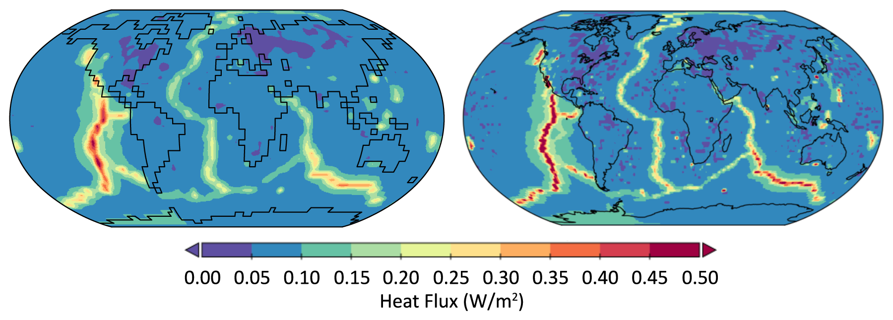
Figure 1Modern Earth geothermal heat fluxes at 4×5° (left panel) and 1×1.125° (right panel) resolutions from a digital 2×2° equal-area map developed by Davies (2013) from a collection of more than 38 000 heat flow measurements from around the world.
2.2.3 Thin atmospheres
If atmospheric pressure at the surface of the planet is significantly lower than the one on modern Earth, then special care should be taken to represent certain processes and to ensure the stability of the model in general. Typically, we consider the atmosphere “thin” if the surface pressure falls below the triple point of water (∼6 mbar). Examples of such planets are modern Mars and planets with transient atmospheres induced by impactors or periods of high volcanic activity (Aleinov et al., 2019). Atmospheres below the triple point of water cannot support liquid water, and while most model algorithms (clouds, precipitation) handle this automatically, a special option is provided to exclude any movement of liquid water in the ground. This option has to be enabled (Appendix B) for proper simulation of the hydrological cycle on such planets.
For thin atmospheres, the ground temperature is mainly determined by the competition of absorbed stellar and outgoing longwave radiation fluxes. As a result, a high-temperature gradient is present between the insolated and shaded parts of the surface. This causes the lower atmospheric temperature to decouple from the ground temperature over the shaded regions due to the very stable stratification near the surface, especially for a radiatively neutral atmosphere. In such cases, the conditions in the lower atmosphere are mainly determined by the sensible heat flux over the insolated regions, which is much lower than other surface fluxes, and special care should be taken to avoid its distortion by numerical artifacts. The algorithms for surface fluxes in ROCKE-3D 2.0 were updated to properly handle such conditions. We also disable the horizontal heat transport in the planetary boundary layer; these fluxes are negligible under thin atmospheric conditions, but they can cause numerical instabilities. At the top of the atmosphere, the atmospheric layers are very thin and may require a very short time step to maintain their stability with respect to radiative heating/cooling. To avoid this problem, we provide an option to treat the upper three layers as isothermal layers by the radiation model (Appendix B). In the current release, the model can handle surface atmospheric pressures down to 10 µbar. This configuration has already been used to simulate a thin CO atmosphere as a likely candidate for a transient volcanically induced paleo-lunar atmosphere (Aleinov et al., 2019; Needham and Kring, 2017).
Depending on atmospheric composition, extremely thin atmospheres may require non-local thermal equilibrium (non-LTE) corrections in the radiation algorithm. These have not been implemented yet and may become available in future releases. For exceedingly thin atmospheres (<10 µbar) non-LTE radiative effects may become important; however, non-LTE physics are not implemented in SOCRATES. For Early Moon simulations we assume CO-dominated atmospheres in which, fortuitously, non-LTE effects are negligible and can be ignored (Forget et al., 2017). However, caution should be exercised that for different atmospheric compositions (e.g., CO2-dominated) non-LTE effects can be important and can have non-negligible impacts on results.
2.2.4 Calendar and equation of time
The calendar facility in ModelE is designed to generate a custom calendar that is tailored to the various exoplanet orbital parameters. With some important caveats that are elaborated on below, the generated calendar maintains a familiar correspondence to conventional Earth-based calendars – e.g., each orbital year is divided into 12 months of varying duration – but integer numbers of days. An attempt is made to align seasons by forcing the vernal equinox to be at the same fraction of the calendar as is the case for the Earth. Each day is divided evenly into 24 h, which is generally different than the expected 3600 s in duration.
To avoid complexities analogous to leap days/years, the rotational period is, by default, quantized to ensure an integer number of days per orbit. More specifically, the rotational period is adjusted in a minimal manner such that the number of rotational periods evenly divides the orbital period. We adjust the rotational period rather than the orbital period, because we generally have superior information about orbital periods of actual observed exoplanets. This quantization can be deactivated, in which case the orbital year and the calendar year are of different durations, which then requires some caution in interpreting some diagnostics, i.e., an “annual mean” quantity might require more than one orbit to properly average out.
The duration of each of the 12 months is determined by a heuristic based upon a reference orbit and calendar for the Earth. More precisely, we determine the longitude relative to the vernal equinox of the start time of each month in the reference 365 d pseudo-Julian calendar used by ModelE for modern Earth simulations. The exoplanet calendar attempts to preserve the same angles for the start times of its months but makes small adjustments to ensure an integer number of days in each month. In this manner, all other things being equal the exoplanet “February” will generally be a shorter month, simply because it is a short month in a conventional calendar. This aspect is easily dominated by other factors for planets with large eccentricities and/or different longitude of the periapsis as compared to that of the Earth.
For exoplanets with a large separation between rotational and orbital periods, the above calendaring system works quite well, but the implementation requires and allows further adjustments to better support slow rotators. By default, the minimum number of calendar days in a year is 120 (roughly 10 per month). For a slow rotator, this means that calendar days will lose direct correspondence with the solar days. This default can be overridden, which can result in months that have 0 d. Further, for extremely slow rotators such as Venus, the quantization of the rotational period mentioned above is too severe, and the implementation therefore provides an option to deactivate the default quantization. In such cases, the calendar is of relatively little use, and useful diagnostics generally require averages over many orbits to avoid day–night biases within any given orbit.
The implementation of the calendar in ROCKE-3D 1.0, or more precisely the calculation of the actual hour angle, did not include the effects due to the equation of time (EOT) which arises due to the difference in the length of a solar day at apoapsis versus periapsis and also the obliquity-induced effect between solstices and equinoxes. For the Earth this effect is minor and not usually included when studying modern climate, but for highly elliptical orbits this effect can be significant (Colose et al., 2021). ROCKE-3D 2.0 corrects this oversight and introduces three options for EOT that can be chosen by the user upon model configuration: “off”, “naïve”, and “default”. The “naïve” option implementation neglects the contributions due to obliquity. This option and “off” are provided for backward compatibility, and we recommend that the correct formula provided by “default” is always used.
2.3 Radiation schemes
Two fundamentally different radiation schemes are available in ROCKE-3D: the first is the GISS radiation (denoted as “G” in our naming convention; Sect. 4), which is strongly optimized for present-day and near-term paleoclimate Earth applications (Kelley et al., 2020, and references therein), and the other is the SOCRATES radiation (denoted as “S”; Amundsen et al., 2016, 2017; Edwards, 1996; Edwards and Slingo, 1996), whose implementation in ROCKE-3D has been presented in Way et al. (2017). The GISS radiation is much faster but has limited applicability and suffers accuracy losses when the atmosphere and incident stellar energy distribution (SED) under study deviates appreciably from that of preindustrial Earth and present-day Sun combination. This is especially important when it comes to making large changes to the amount of atmospheric absorbers (e.g., H2O, CO2, CH4), when it comes to making large changes in the temperature profile, and when using SEDs from cool stars where the peak in radiation is shifted into the near-infrared. SOCRATES, on the other hand, is much more flexible and can simulate different atmosphere and SED combinations very easily, albeit with preprocessing requirements to create the so-called “spectral file”. A spectral file is a construct native to SOCRATES which contains all aspects of the radiation problem, including the spectral interval and Gauss point grids, gas absorption coefficients for major and minor species, Rayleigh scattering coefficients, cloud optical properties, and aerosol optical properties. Different spectral files can be fed in to SOCRATES at runtime, meaning that the radiative transfer problem can be defined for numerous diverse atmospheres without needing to modify the code and recompile SOCRATES. Generally, better accuracy for more exotic star–atmosphere combinations requires increasing the density of spectral intervals and Gauss points, which results in a slower runtime performance (also see Sect. 4.5). However, the speed reduction is necessary to obtain highly accurate radiative transfer results for the variety of atmospheres that can be studied with ROCKE-3D. All simulations presented here use the ga7_dsa spectral file (Appendix C).
The motivated user can create their own unique spectral files using a set of shell and Python scripts provided publicly on GitHub (see “Code availability”), which wrap native SOCRATES routines for creating and manipulating all components of the spectral file. However, as part of ROCKE-3D, we provide numerous pre-computed spectral files, which should satisfy the requirements of most use cases (see “Data availability”). These are divided into several general classes based on the atmospheric composition which they serve, referencing Earth and Mars time periods. Each class has numerous spectral files optimized for specific subsets of the atmospheric composition. As the name implies, “Modern Earth” spectral files are only appropriate for modern Earth atmospheric compositions and temperature ranges, while allowing for increases and decreases by several doublings of CO2 or CH4. “Archean” spectral files have been constructed to incorporate high amounts of CO2 and CH4 in an N2-dominated anoxic atmosphere while allowing total pressures up to 10 bar. The “Paleoproterozoic” spectral file includes a combination of low O2 and moderately elevated CO2 and CH4 in an otherwise N2-dominated atmosphere. We use “Mars through time” to describe spectral files which feature CO2-dominated anoxic atmospheres, valid for modern Mars but also any generic dense CO2 atmosphere (Del Genio et al., 2019b; Guzewich et al., 2021; Schmidt et al., 2022). We have also constructed additional spectral files for other worlds, including Titan and a putative early lunar atmosphere (Aleinov et al., 2019). Stellar spectra have been constructed for numerous stars ranging from ultracool M-dwarf stars to late F-dwarf stars. An at-length description of the technical details of the currently available spectral files and stellar spectra is included with our publicly available materials (ROCKE-3D spectral files). Refer to Appendix C for additional information.
2.4 Atmospheres
In ROCKE-3D 1.0 we only provided template configurations for one type of atmosphere – that of preindustrial Earth but without atmospheric aerosols, O3, and stratospheric formation of H2O from CH4 oxidation. In ROCKE-3D 2.0, in addition to the ROCKE-3D 1.0 atmospheric configuration (denoted as “x” in our naming convention; Sect. 4), we added two additional template configurations: one (denoted as “A”) is the exact atmosphere of preindustrial Earth for the year 1850 and the other (denoted as “N”) is the same atmosphere but without aerosols, O3, and stratospheric formation of H2O from CH4 oxidation and with the O2 and Ar of the atmosphere replaced by N2. This makes the N configuration essentially a pure N2 atmosphere, except for trace components present like CO2 and N2O, both of which are at their preindustrial Earth levels. ROCKE-3D can run using a wide range of additional compositions, e.g., pure CO2 (Mars), pure CO or N2 (Aleinov et al., 2019), and mixtures of non-condensable gases.
2.5 Oceans
The ocean parameterization chosen is very important in the simulated climate of any planet with a substantial ocean present. In Earth's modern climate, most of the poleward heat transport occurs in the atmosphere except in the deep tropics (Held, 2001; Klinger and Marotzke, 2000; Trenberth and Caron, 2001). Nonetheless, numerous studies have demonstrated a very strong coupling between the sea ice margin and convergence of ocean heat transport at higher latitudes (e.g., Aylmer et al., 2020; Bitz et al., 2005; Ferreira et al., 2011; Rose et al., 2013; Winton, 2003). For exoplanets, the effect of ocean dynamics can produce results that are qualitatively far different than that assuming Q-flux = 0 (Del Genio et al., 2019b; Hu and Yang, 2014). Most notably, on synchronously rotating worlds, the presence of a dynamic ocean can expand the area of deglaciated ocean on planets near temperatures where sea ice is expected to form. Generally, a dynamic ocean forms what is termed a “lobster pattern” in temperature, while a Q-flux = 0 ocean forms an “eyeball” world (e.g., Pierrehumbert, 2010; see also Fig. 2a and b in Del Genio et al., 2019b).
As in ROCKE-3D 1.0, three ocean configurations are available. The first configuration (prescribed sea surface temperature (sst); denoted as “p” in our naming convention; Sect. 4) has no interactive ocean but rather a prescribed sea ice extent and sst. Although no ocean calculations happen in this configuration, the ocean heat transport is implied and is equal to that of preindustrial Earth. The second (Q-flux; denoted as “q”) is a Q-flux ocean (Miller et al., 1983; Russell et al., 1985), in which (contrary to ROCKE-3D 1.0 where we used Earth-like heat fluxes) the heat fluxes throughout the ocean are set to zero. This is a common assumption in exoplanet studies with important consequences to the simulated climate, as shown here. In this model setup the atmosphere and sea ice are coupled to a mixed-layer ocean of a specified depth, which allows for time-varying storage and release of heat, as well as a source of evaporation to the atmosphere. The depth of the Q-flux = 0 ocean in ROCKE-3D 2.0 is 100 m (the default value was 65 m in ROCKE-3D 1.0), and it is trivial to change to any desired depth. The last configuration (dynamic ocean; denoted as “o”) is a fully dynamic ocean, similar to what was used in ROCKE-3D 1.0, with present-day Earth's bathymetry, but any configuration can be used, e.g., a bathtub ocean with flat bathymetry used in aquaplanet (water world) simulations (Sect. 4.4.4). The initial conditions used are based on present-day Earth's modern ocean configuration (Levitus et al., 1994; Levitus and Boyer, 1994).
2.6 Grid resolutions
The Earth version of ROCKE-3D, ModelE2.1, is routinely run in the fine horizontal atmospheric resolution of 2×2.5° in latitude and longitude, denoted as “F” in our naming convention (Sect. 4), with 40 horizontal layers to 0.1 hPa. This model version is coupled to a dynamic ocean with a 1×1.25° resolution in latitude and longitude and 40 layers to the ocean floor. Virtually all studies done thus far with ROCKE-3D have been performed at medium resolution (denoted as “M”), using either 40 or 20 atmospheric vertical layers and a 4×5 ocean with 13 layers. In ROCKE-3D 2.0 we only kept the 20-layer atmospheric model version as a legacy (working but unsupported) option and opted to use for all simulations the 40-layer atmospheric version. We also decided to include the M and F resolutions in order to be able to resolve with greater accuracy larger-than-Earth planets and fast rotators.
2.7 Template model configurations
In ROCKE-3D 1.0 (Way et al., 2017), we provided template configurations for an Earth-like atmosphere with conditions similar to preindustrial Earth (year 1850), but with zero aerosols, ozone (O3), and stratospheric water vapor formation from methane (CH4) oxidation. In ROCKE-3D 2.0 we expanded the available options offered, which now include combinations of two radiation schemes, three different atmospheres, three ocean configurations, and two horizontal resolutions, resulting in a total of 36 supported configurations. Here we will describe the reasons that led us to the choice of such configurations, the decisions made to balance them, their differences, and their limitations. Their naming convention is presented in Fig. 2, which is the one used in the code repository and here, and a detailed discussion of their resulted climates will follow in the next sections.

Figure 2Template configuration naming convention. For the meaning of the letters, see Table 1. As an example, a fine-resolution configuration of preindustrial Earth atmosphere with a dynamic ocean and GISS radiation is named P2GApF40.
Table 1ROCKE-3D version 2.0 template configuration naming convention explanation.
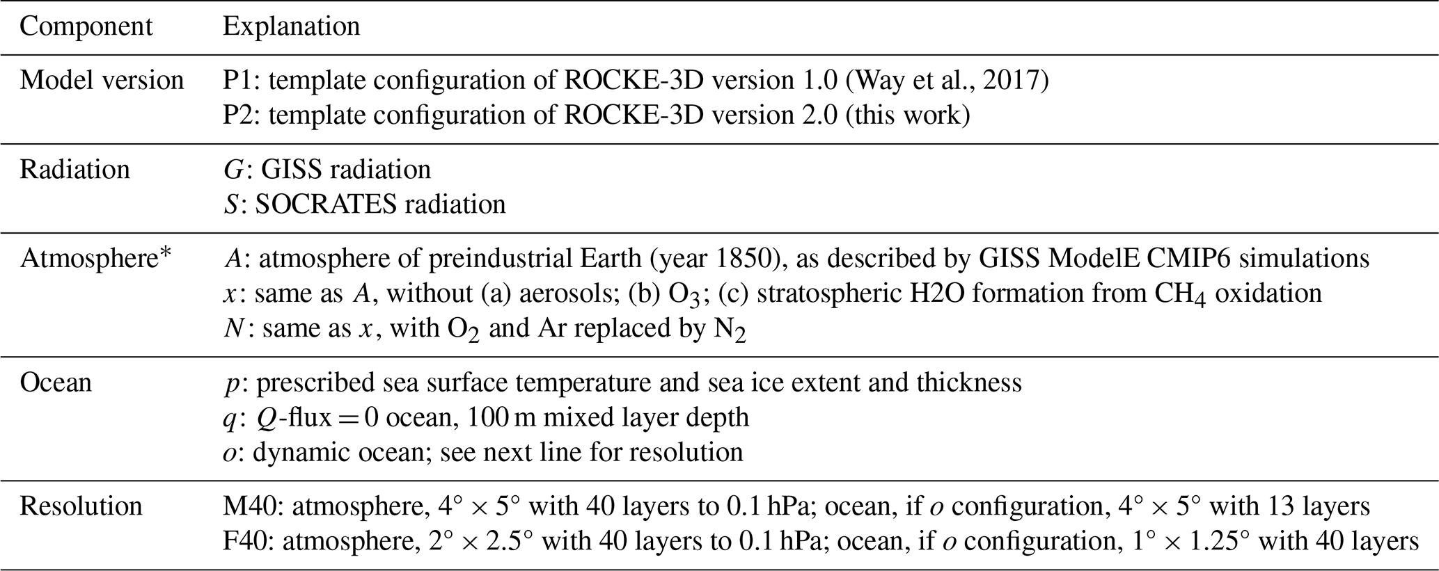
* In the text these configurations are frequently named Earth (A), ROCKE-3D 1.0 (x), and anoxic (N) atmospheres.
In this work, the GCM variable names of the model output are abbreviated for many quantities, rather than a more verbose explanation. This helps the model user to exactly understand which model output we have used in our analysis but also to detail which variables are important to analyze when creating a new world. These variables are explained in Appendix D.
3.1 Radiative balance
Bringing the model into radiative balance is a necessary step to create a control simulation in which temperature, as well as shortwave and longwave fluxes, is acceptably close to target values. There are multiple ways one can calibrate the model to achieve this. Our method is to bring the model into radiative balance under preindustrial conditions (described in Sect. 4.1), for which we use a prescribed ocean configuration and make changes to cloud parameters so that the absolute value of the net incoming stellar and outgoing thermal radiation of the whole planet (net_rad_planet) is small (within ±0.2 W m−2). For Earth-centric science questions, a secondary goal is that the present-day net radiative balance of the planet is on the order of +1 W m−2, but this is not relevant to this work, which focuses on a generalized planetary configuration rather than the current state of the planet and the impact humans have on it. It is important to note that not all configurations can easily (if at all) stay within those limits, mostly because when deviating from the actual preindustrial Earth there is no “real” ocean field to be used, so the atmosphere might take much longer, or even fail, to fully adjust. This will be discussed later, on a case-by-case basis, when it occurs.
There are other, secondary criteria that also need to be loosely met which are known for the present-day atmosphere but can only be estimated for the preindustrial one. These include global mean surface air temperature (tsurf; 14–15 °C at present day, roughly 1 °C cooler at preindustrial), planetary albedo (plan_alb; about 29.6 % at present day, unknown at preindustrial), stellar (shortwave) radiation net flux at the top of the atmosphere (srnf_toa; 239±2 W m−2 at present day, probably the same at preindustrial), and ocean sea ice fraction (oicefr; 4 % at present day, slightly greater at preindustrial). When balancing the model, we always try to have |net_rad_planet W m−2 while trying to also maintain srnf_toa as close as possible to 239±2 W m−2 by modifying the radiative balancing factors of clouds (see Sect. 4.1).
We only balanced the model for configurations of interest for the public release of the model. Intermediate configurations use balancing values which might or might not bring the model to radiative balance, depending on how much different model physics affect the modeled climatologies. In Sect. 3.3 below, some model runs will clearly be out of radiative balance by design.
3.2 Effects of new physics on mean climatology
We checked whether the code merges across the Earth (Sect. 2.1) and planetary (ROCKE-3D 2.0; Sect. 2.2) model versions affected the mean climatology of the model in any significant way. For this, we simulated both the year 2000 and year 1850 climatologies by performing 30-year simulations with the prescribed ocean (p) model: the first 10 years were used as a spinup, and the latter 20 were used for the analysis. This is twice as many years as we typically use for balancing the Earth model (both spinup and analysis); we decided to use more years than usual as an additional layer of safety, and as expected it was proven to be unnecessary. The set of simulations performed for the year 2000 showed that all key diagnostics mentioned in Sect. 3.1 are both within bounds and extremely close to each other across model versions, ensuring that the merging process was successful. The same applies for the 1850 climatology across model versions, where all simulations showed that they are in radiative balance. From now on, all simulations discussed are done with the merged product, ROCKE-3D 2.0, and with 1850 base climatological conditions.
There are two major changes that as expected introduced major changes in the model physics and require rebalancing: the change from GISS radiation to SOCRATES (using the ga7_dsa spectral file; Appendix C) and the coarsening of the default Earth resolution from F40 to M40. Note that the M20 resolution used in ROCKE-3D 1.0 is not supported anymore. When SOCRATES is used, net_rad_planet decreases by 1.3 W m−2 and srnf_toa decreases by 6 W m−2. When changing resolution from F40 to M40 net_rad_planet increases by 0.8 W m−2 for GISS and by 0.2 W m−2 for SOCRATES radiation, while srnf_toa decreases by 2.0 and 2.6 W m−2, respectively.
The change in resolution includes not only the physical change of grid box sizes, but also the replacement of the gravity wave drag parameterization from that used on the Earth version of the model (Kelley et al., 2020), with the simpler “Rayleigh friction” version used in ROCKE-3D 1.0 (Way et al., 2017). Structurally, the M simulations employ a simplified version of Rayleigh friction, which exponentially decays wind components over a user-specified range of layers near the model top. The simplification is to apply a user-specified exponential time constant per layer. This replaces the parameters traditionally associated with momentum loss to a solid surface (e.g., drag coefficient, air density, and quadratic dependence upon wind speed). Furthermore, the Earth-oriented version has a special tuning of its Rayleigh friction near the poles; this was especially important for getting the correct stratospheric wind structure in M configurations, because they completely lack the parameterized gravity wave momentum transports that shape stratospheric winds in later model generations (F resolution). This geographic adjustment is dropped in non-Earth-oriented simulations. An even further improved version of the gravity wave drag that is present in the high model top version of the Earth model (Rind et al., 2020) will become available in the next release of ROCKE-3D, but again only for the F model resolution, not M, and with many more than 40 layers (102 in Rind et al., 2020). When using the F40 resolution with the simplified gravity wave drag, the net_rad_planet change for GISS (SOCRATES) radiation is −0.46 (−0.50) W m−2, and the corresponding change for srnf_toa is −0.24 (−0.29) W m−2.
Another necessary change between resolutions is the time step used in the Shapiro filter, which is a hyperdiffusion operator that is applied to remove numerically induced high-frequency noise from the velocity and tracer fields (Shapiro, 1970, 1975): in the fine (F40) resolution this is 225 s, while in the medium resolution (M40) it is 450 s. This change has only a marginal impact in the key diagnostics net_rad_planet and srnf_toa.
3.3 Creation of a generalized Earth configuration
ModelE2.1 contains a control configuration which is meant to simulate preindustrial Earth (year 1850; E2.1GApF40_1850). This contains some Earth-centric parameterizations, each for a different reason, that are not valid for use in other planetary configurations. In ROCKE-3D 1.0 such configurations also existed, but the changes from the tight Earth configuration to the more general one were not studied systematically. Here we present in detail which options we have either eliminated or generalized, as well as their individual impact on model results, towards the creation of the several supported template configurations in ROCKE-3D 2.0, described in Sect. 4. We focus on the net planetary radiation (net_rad_planet) and the stellar (shortwave) radiation net flux at the top of the atmosphere (srnf_toa). Box-and-whisker plots of those diagnostics for the 20 years of the simulation (following 10 years of spinup) are presented in Fig. 3. It is important to mention that many of the differences discussed here would have been reduced by rebalancing the model, but since these are interim simulations that are not meant to be used for production, the absolute values of such differences do not matter much.
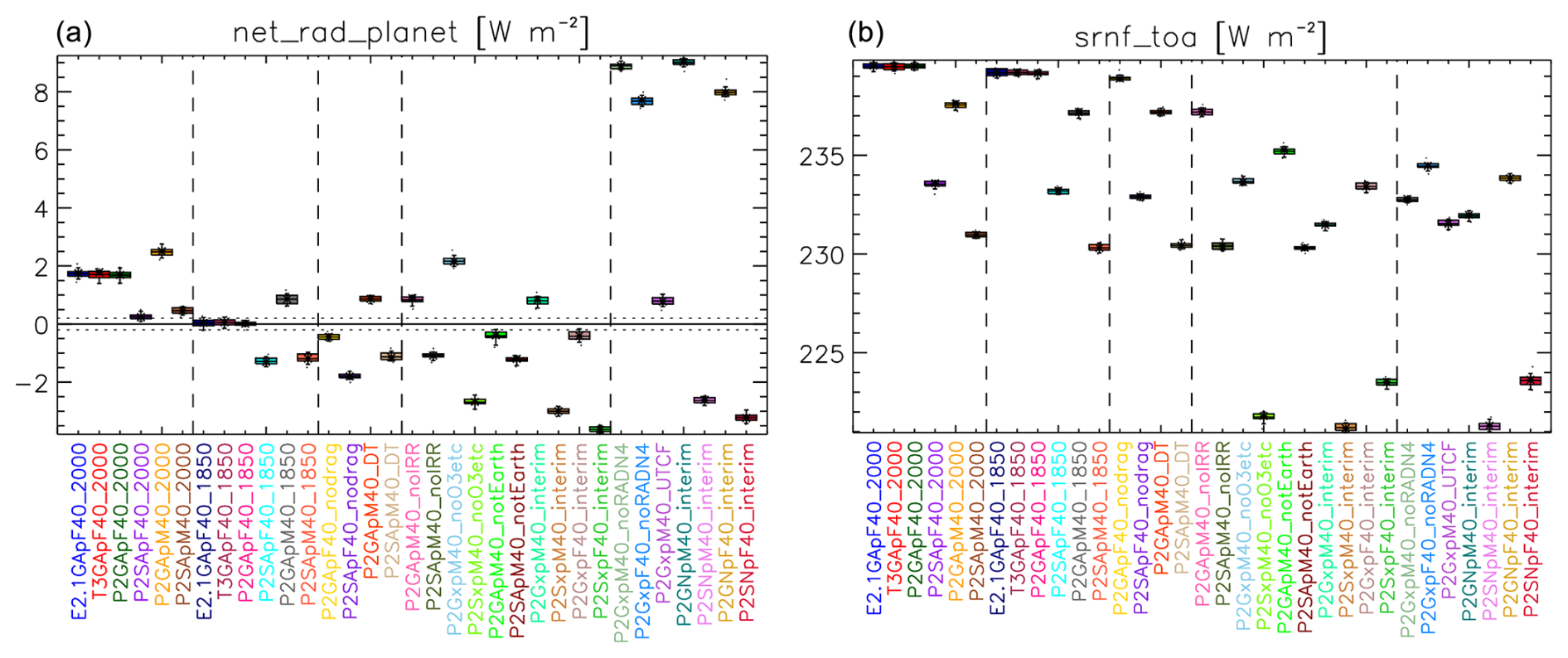
Figure 3Box-and-whisker plots of net planetary radiation (net_rad_planet; a) and stellar (shortwave) radiation net flux at the top of the atmosphere (srnf_toa; b) for the intermediate simulations described in Sect. 3.3. The part of the simulation names before the underscore is explained in Sect. 3, with the addition that E2.1 and T3 mean the default and the updated ModelE2.1 version of GISS ModelE, respectively. For the part after the underscore, see Table 2.
After having constructed preindustrial Earth model configurations for all combinations between fine and medium resolutions, as well as GISS and SOCRATES radiations, the next goal was to set up configurations for uninhabited planet simulations. These primarily included configurations that do not include irrigation, aerosols, and O3, but also other changes related to clouds (P2GApM40_notEarth in Table 2). We quantified the difference they introduce to srnf_toa, and by assuming linearity in responses (in the absence of a better assumption), we modified our target srnf_toa value from 239±2 W m−2 (Sect. 3.1) for the radiative balancing to a new value, as described below. All simulations have been performed with the M40 resolution, which is anticipated to become the most used one.
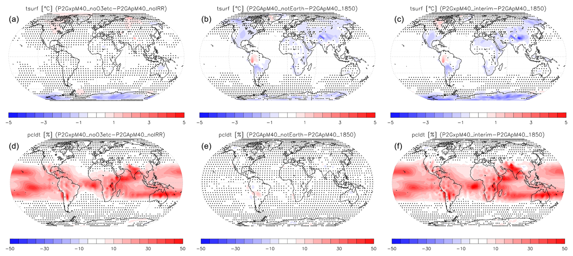
Figure 4Surface temperature (a–c) and total cloud fraction (d–f) change due to the removal of aerosols, O3, and stratospheric water vapor from CH4 oxidation (a, d), some Earth-centric corrections (including the cloud top limit; see text and Table 2; b, e), and the combination of the two (c, f). Note that panels (c) and (f) also includes the effect of irrigation removal, which is statistically insignificant in the preindustrial atmosphere used here. Dots show grid boxes where the calculated differences are not statistically significant (p>0.05).
Table 2Description of intermediate simulations described in Sect. 3.3 with the GISS radiation. All configurations that start with P2G in the table were also performed using the SOCRATES radiation instead of GISS, in which case we replace G with S in the name, e.g., P2GApM40_1850 becomes P2SApM40_1850, but are omitted below for brevity.
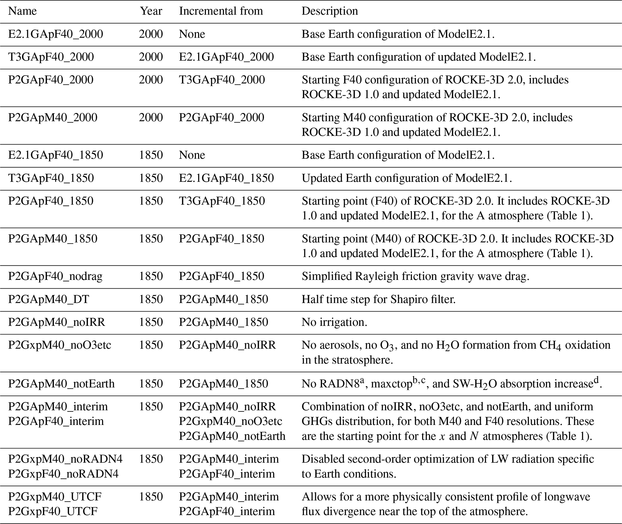
a Earth-centric cloud inhomogeneity correction, but instead using a constant value of 0.12. b CPU-saving setting which skips cloud calculations above a fixed pressure level (50 hPa for Earth). c This is the only change that is relevant for SOCRATES in P2SApM40_notEarth. d Shortwave long-path H2O absorption increase.
The removal of irrigation does not produce any noticeable change in net_rad_planet and srnf_toa. The same applies to key diagnostics like surface temperature and total cloud fraction, where any regional changes calculated are not statistically significant. On the other hand, and as expected, removing aerosols, O3, and the formation of H2O in the stratosphere by CH4 oxidation produces a large change in net_rad_planet for GISS (SOCRATES) radiation of +1.33 (−1.60) and a change of −3.5 (−8.7) W m−2 for srnf_toa. The large difference of srnf_toa between the two radiation schemes leads to a very different response in clouds, which results in a net_rad_planet change of a different sign between the two model configurations. Regionally, the removal of aerosols, O3, and stratospheric H2O from CH4 oxidation completely dominates the change in total cloud cover. Cloud cover increases throughout the tropics by as much as 60 % locally but changes less than 5 % anywhere else (Fig. 4). It also has some statistically significant impact on tsurf at polar latitudes and in particular in Antarctica, but the effect is overall smaller than the removal of Earth-centric adjustments (P2GApM40_notEarth in Table 2) that cause a cooling of surface temperatures over land almost everywhere, which largely dominates the net effect of both changes (Fig. 4). Over the ocean the changes in tsurf are negligible, primarily because we use the prescribed ocean configuration (p) which does not allow changes to sst, a major driver to tsurf. It has to be noted that the choice of atmospheric composition described here (no ozone, aerosols, and stratospheric water vapor from methane oxidation; x configuration in Table 1) was made for consistency with the ROCKE-3D 1.0 non-Earth configurations. We decided to keep that legacy configuration in ROCKE-3D 2.0 for continuity, although it contains inconsistencies, in that the atmosphere contains O2 but not O3. We also created a set of configurations in ROCKE-3D 2.0 (anoxic Earth) that eliminate that inconsistency, which we recommend to be the default one for future studies. More on this in Sect. 4.
In another simulation generalized for non-Earth simulations, we removed a clouds heterogeneity parameterization whose spatial distribution is relevant for Earth only (first introduced in ModelE by Schmidt et al., 2006) and used a constant factor instead. This factor scales the cloud optical depth down to account for the fact that variable optical depth within a partially cloudy grid box causes shortwave extinction to be less than what one would get from a homogeneous cloud. ModelE uses a map of the inhomogeneity correction appropriate to Earth from the International Satellite Cloud Climatology Project (ISCCP) D1 cloud climatology (Rossow et al., 2002). In order to not impose an Earth-like pattern of inhomogeneity, we used instead a global mean value of 0.12 (see Appendix B for technical instructions). In addition, we removed a shortwave long-path H2O absorption increase, which was found to be necessary for Earth simulations to correct an underestimate of the direct and diffuse shortwave H2O band absorption analytical fit used in the GISS radiation when compared against measurements, particularly for high-humidity cases. All of those changes are only relevant when using GISS radiation, not SOCRATES. We also allowed the cloud code to run up to the model top (0.1 hPa) instead of up to 50 hPa, a limit inspired by present-day Earth and set for computational efficiency. Other atmospheres, especially those without a stratospheric temperature inversion, might have clouds much higher than where they exist on Earth, so removing this Earth-centric limit is important. This change is relevant for both GISS and SOCRATES simulations. The GISS radiation simulation with those adjustments removed resulted in a change in net_rad_planet of −1.27 W m−2 and a change in srnf_toa of −1.9 W m−2. As expected, these changes require the model to be rebalanced. The cloud change (allow them to reach the model top) in the SOCRATES simulation did not change either of the diagnostics beyond noise, since no clouds are expected to exist above 50 hPa. Although no incremental simulation with the clouds allowed to reach the model top was performed using the GISS radiation, it is expected that it will not affect the climatology, as was the case for SOCRATES.
After having tested all changes from the standard preindustrial Earth configuration, we combined all pieces together and generated a candidate configuration for radiative balancing, for both radiation schemes and for both resolutions. These are the interim simulations in Table 2. For the GISS radiation, the total srnf_toa change for both resolutions is −5.7 W m−2, while for SOCRATES it is a bit over −9 W m−2 (−9.1 for M40 and −9.7 for F40). For the GISS radiation this net change adds up pretty linearly to the individual changes caused by the elimination of O3 and aerosols (−3.5 W m−2) and adjustments in radiation (−1.9 W m−2). For SOCRATES, the change from O3 and aerosols is −8.7 W m−2 (no Earth-specific adjustments exist to be eliminated), which is also very close to the net effect of M40 (−9.1 W m−2). The net_rad_planet for the GISS radiation ends up pretty well balanced for M40 (−0.06 W m−2), probably by chance, while it is 0.4 W m−2 for F40. SOCRATES is further away from radiative balance, with −1.8 and −2.3 W m−2 net_rad_planet for M40 and F40, respectively.
As a last configuration test for the GISS radiation only, we removed a longwave correction (noRADN4 in Table 2), which we will only keep enabled in the atmospheres that exactly resemble modern Earth, and also enabled a more physically consistent profile of longwave flux divergence near the top of the atmosphere (Appendix B). The longwave correction introduces a major radiative imbalance of +8.1 W m−2 for both resolutions and a +1.0 W m−2 (M40) and +1.3 W m−2 (F40) change in srnf_toa, while the longwave flux divergence, probably the least impactful modification, only marginally changed results.
3.4 Analysis of additional diagnostics
Although net_rad_planet and srnf_toa are key diagnostics that affect the simulated climate of any atmosphere, there are many more diagnostics one can examine and understand differences between simulations. A key set of those, but by no means an exhaustive one, is compared against the default preindustrial configuration of ModelE2.1 in Fig. 5. A key conclusion is the confirmation that virtually all Earth configurations across model versions (ModelE2.1 (E2.1GApF40_1850), ModelE2.1 with updates (T3GApF40_1850), ROCKE-3D 2.0 starting point (P2GApF40_1850), and final ROCKE-3D 2.0 generalized configuration (P2GApF40); also see Table 2) produce the same climatology. These are marked with a blue arrow in Fig. 5, where there are practically no differences between the simulations.
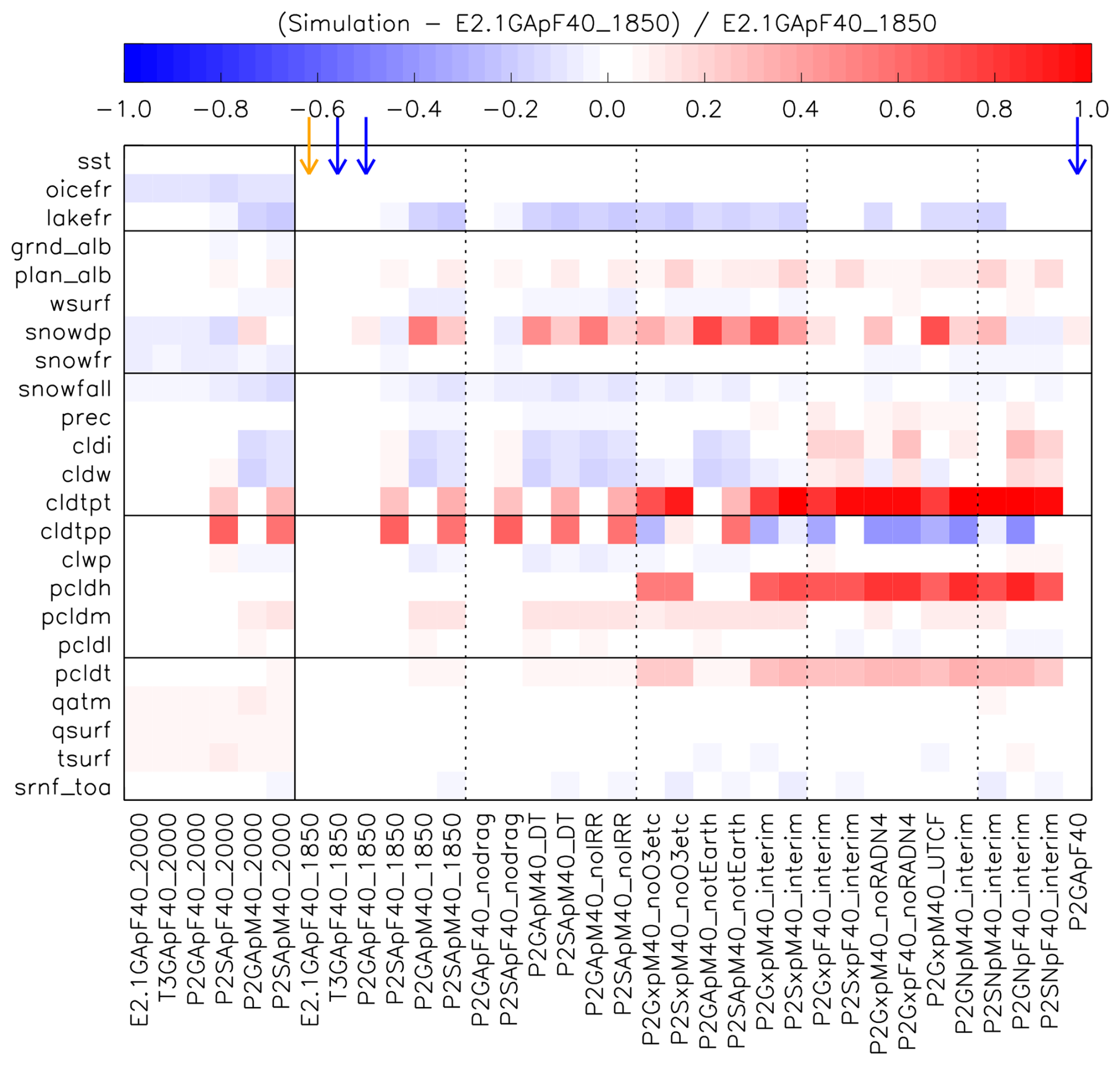
Figure 5Relative differences of key diagnostics of the intermediate simulations listed in Table 2 compared to the original preindustrial Earth simulation in ModelE2.1, marked with an orange arrow. Exactly equivalent simulations with different model versions (see text for details) are marked with blue arrows. Remember that most of the simulations presented here are not in radiative balance. Diagnostics are the following: sst – sea surface temperature; oicefr – ocean ice fraction; lakefr – lake fraction; grnd_alb – ground albedo; plan_alb; planetary albedo; wsurf – wind speed at surface; snowdp – snow depth; snowfr – snow fraction; snowfall – snowfall; prec – precipitation; cldi – cloud condensed ice column; cldw – cloud condensed water column; cldtpt – cloud top temperature; cldtpp – cloud top pressure; clwp – cloud liquid water path; pcldh/pcldm/pcldl/pcldt – high/middle/low/total cloud cover; qatm – atmospheric water vapor column; qsurf – surface air specific humidity; tsurf – surface air temperature; srnf_toa – net stellar radiation at the top of the atmosphere. See Appendix D for more details.
A number of interesting patterns emerge when looking at the other simulations, which will be only briefly discussed here. Those simulations are not in radiative balance (Fig. 3), due to their intermediate nature, as mentioned earlier. First of all, the year 2000 simulations are slightly warmer as expected, which results in less ocean ice (oicefr) and reduced snowfall rate and snow amount (both depth and fraction). The warmer temperature also allows the atmosphere to hold more moisture at surface and in the column. Another persistent pattern is for the year 1850 simulations with SOCRATES, which calculate warmer cloud top temperatures and higher pressures, implying that clouds reach higher altitudes when using the GISS radiation. Further, the simulations without O3 are cloudier, in particular in the higher-altitude cloud region. This is mostly due to the increased presence of ice clouds, a result of colder temperatures from the middle troposphere and upwards. Also note that these simulations do not have a stratospheric temperature inversion, due to the absence of O3, as further discussed in Sect. 5. The cloudier atmosphere also results in an increase in the planetary albedo.
4.1 Radiative balancing per configuration
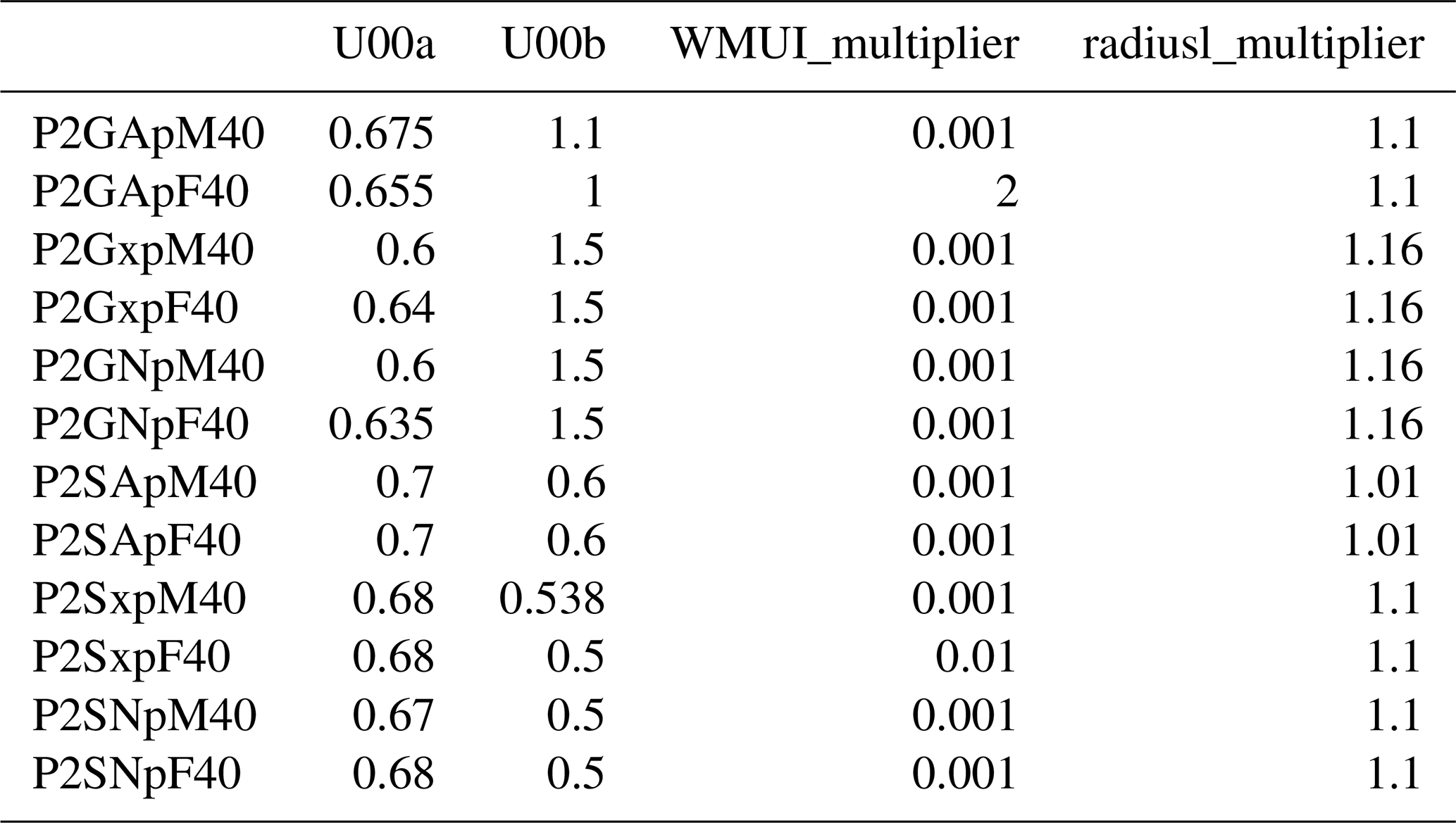
For preindustrial conditions, Earth is assumed to be very close to radiative balance, meaning that the absorbed shortwave stellar radiation is approximately equal to the outgoing longwave radiation at the top of the atmosphere, to within a few tenths of a W m−2, in the range 240±5 W m−2. For the various configurations of ModelE2.1, small variations of a single parameter (U00a) have sufficient differential impacts on SW and LW to serve as the final rebalancing mechanism, after previous tuning steps set U00b, WMUI_multiplier, and radiusl_multiplier. In the search for radiative balance across the multiple configurations of ROCKE-3D 2.0, the four parameters were not required to remain close to one another across configurations or to ModelE2.1 values. This freedom was taken to be justified due to the differences in resolution, radiation scheme, etc. being considered major rather than minor perturbations to the system. Table 3 lists the results. A short explanation of these variables is presented in Appendix D, while more detailed explanations of some of them have been presented elsewhere (Kelley et al., 2020; Schmidt et al., 2006). Note that the appropriate name for U00a and U00b is Ua and Ub, respectively, and this name has been used in past publications, but we opted to use the variable name found in the model code here, similar to what we do with other quantities discussed throughout the paper.
Table 3Radiative balancing parameters of clouds for all p ocean configurations that bring the model to radiative balance. Two additional balancing knobs exist, WMU_multiplier and radiusi_multiplier, but both equal to 1 in all configurations, so they are omitted from the table for clarity.
For every model configuration, a new radiative balancing is likely to be required. We call this “balancing”, because we modify some key cloud-related properties in order to achieve radiative balance in the model, based on our best known configuration of a radiatively balanced case – that of preindustrial Earth (year 1850; Sect. 3.1). These are not unique choices, as there is more than one way to achieve radiative balance in the model, all of which are more or less equivalent. For this we use the p ocean (Table 1) in order to let the atmosphere adjust to the best known state of the ocean at preindustrial times. After allowing the model to radiatively equilibrate for about 10 simulation years, we continue the simulation for 20 more years, which we average for evaluation. When changes were needed, we performed them (not shown; only the final chosen values are presented in Table 3) and repeated the 30-year simulation. When the configuration is in radiative equilibrium (the planet neither gains nor loses energy, averaged over 20 years), we perform a 500-year simulation (a complete overkill, but for consistency with the other simulations) and average the last 100 years for the analysis presented here. This was done for all 12 simulations with the p ocean: (2 radiation schemes) × (3 atmospheres) × (2 resolutions). The balancing factors for each of the p oceans were then used for the similar configurations where the ocean was either q or o (Table 1), without any further adjustments. The final values per configuration are listed in Table 3, and their explanation can be found in Appendix D.
The use of a prescribed ocean in the balancing is necessary, because otherwise the ocean will try to absorb (or give back) the excess heat (or deficit) when net_rad_planet is positive (negative). This means that for a different configuration, one should either use a proper sst data set for the balancing or, in the absence of one, use a Q-flux or dynamic ocean and select the balancing parameters from the atmosphere that is closer to the one under study.
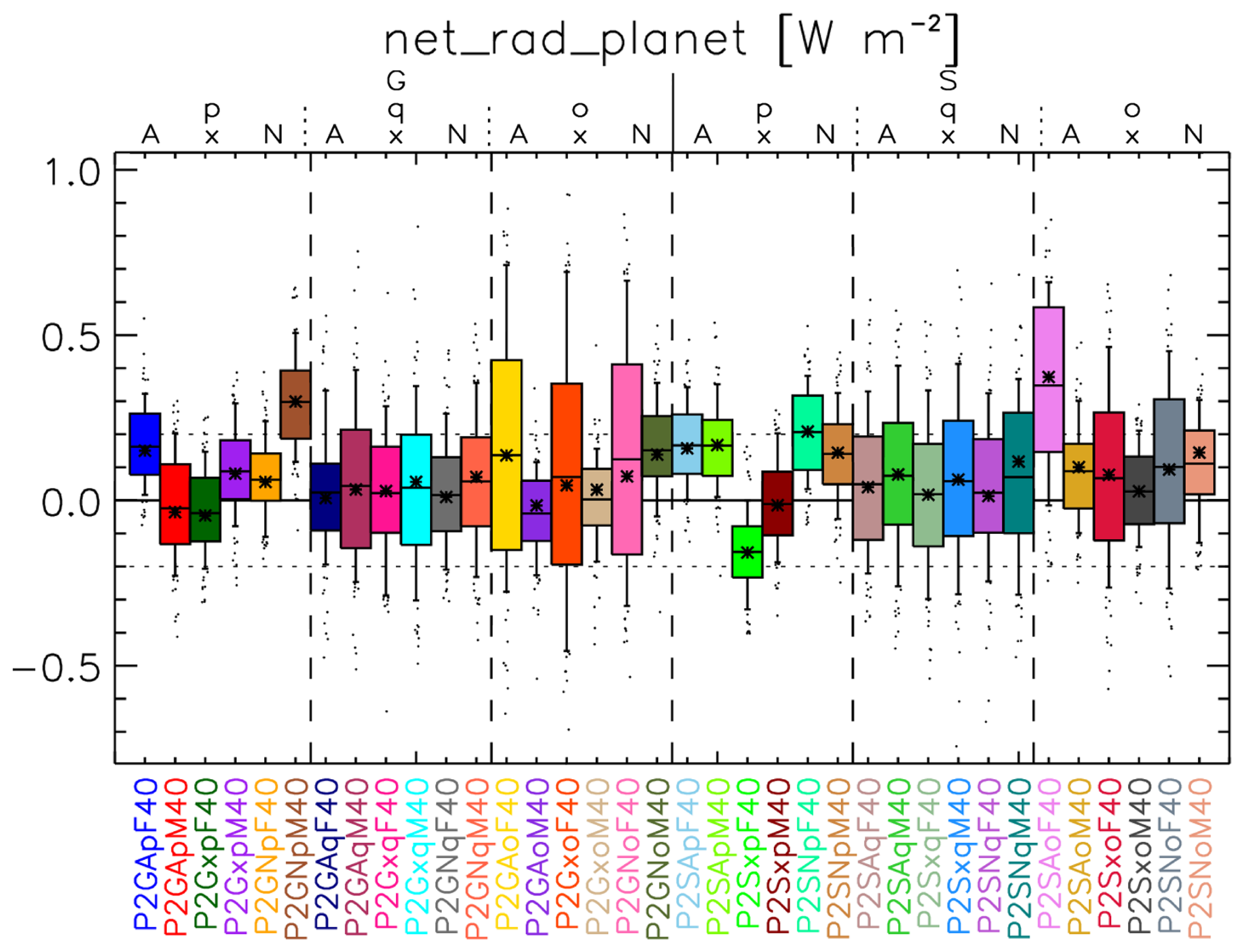
Figure 6Box-and-whisker plot of net planetary radiation (net_rad_planet) in W m−2 for all ocean configurations following balancing. The last 100 years of 200- to 500-year-long simulations were used for the p and q ocean configurations, which were longer (1000 to 2000 years) for the o ocean. The bars show the 25th–75th percentiles, the whiskers show the 9th–91st percentiles, the bar is the median, the star is the mean, and outlier years are presented with dots. Also shown are the ±0.2 W m−2 values, described in the text.
It has to be stressed that we do not have any such information to perform a proper balancing on any non-modern-Earth planet; one has to rely on the values for Earth and pick the closest set to the new planet configuration. If that planet has an ocean, we will not know its sst in the foreseeable future to balance radiation in the same way, so using a dynamic ocean is strongly recommended. Picking a set of values that structurally make sense from Table 3 (i.e., based on which radiation scheme, atmosphere, and resolution would be used) and then allowing the dynamic ocean to adjust as needed is the only feasible approach.
Following balancing, all model configurations have absolute net_rad_planet values either nearer zero or very close to the ±0.2 W m−2 range (Fig. 6). It is interesting to note that all simulated atmospheres using the GISS radiation, dynamic ocean, and fine resolution (P2G[AxN]oF40) have a much larger variability than any other combination of physics, while their corresponding simulations using the medium resolution (P2G[AxN]M40) have among the least.
The balanced P2GApF40 simulation is in all climate-relevant respects the same as ModelE2.1 E2.1GApF40_1850, which is the most heavily tested configuration of GISS ModelE when a prescribed ocean is used (Sect. 3.4). Some regional differences across the model simulations are very minor, which confirms that the model skill and mean climatology do not change with the updated code in ROCKE-3D 2.0 when compared with ModelE2.1.
4.2 Bringing the model to equilibrium
When simulating an atmosphere of any configuration on any given planet, ROCKE-3D needs some time to produce a stable climate for a climatological analysis. The time needed to arrive to equilibrium varies based on the atmosphere, ocean, and land to be simulated; the resolution; and the deviation of initial conditions from the final equilibrium. There are different metrics that define when the model is in equilibrium, which in general might depend on the needs of each individual experiment, since different components of the model equilibrate at different timescales. These timescales can vary from very few years for an atmosphere similar to present-day Earth and a prescribed ocean to centuries for biogeochemical carbon cycling involving land and ocean biology (Jones et al., 2016; Séférian et al., 2020) to several millennia for surface hydrology and a dynamic ocean (van den Hurk et al., 2016; Johns et al., 1997; Sitch et al., 2015; Wood, 1998). For a planet with an abundance of water, even in the absence of an ocean, surface hydrology equilibration times can also be at the several millennia timescales, to allow deep soils to come into full equilibrium. The same applies for dynamic ocean configurations which are several kilometers deep. The simulations listed in Table 2 are with a prescribed ocean, and the water cycle does not need to be in complete equilibrium for the radiative equilibration of the atmosphere, so a few years are enough. The metrics used as criteria of an equilibrated climate also vary depending on the research question. Here, we want the net radiation of the planet to be near zero (within ±0.2 W m−2) in a long climatological mean over several years (orbits, for non-Earth planets) and also to have surface air temperature stabilized.
All simulations presented in Table 3 start with a correct set of balancing parameters for the underlying ocean (Sect. 4.1), so they are in near-instant equilibrium (just a few years). For the Q-flux and dynamic oceans, although using the correct balancing parameters, they are not in equilibrium at the beginning of the simulation because of imperfect parameterizations and forcings that cannot exactly reproduce the prescribed ocean conditions. The Q-flux ocean takes much longer than the prescribed ocean to reach equilibrium, about a century in ROCKE-3D 2.0 or 20 years in ROCKE-3D 1.0, while for the dynamic ocean it takes a millennium or more: about 1500 using the medium resolution and 1000 for the fine resolution (Fig. 7). Note that even after 2000 years, not everything is in perfect equilibrium, but having some very-slow-equilibrating variables still drifting does not affect the other climatological parameters that have already been equilibrated. For a deep dynamic ocean the time for full oceanic equilibrium (e.g., a stable global potential temperature) can take many thousands of years (Fig. 8). Another example is the total amount of liquid freshwater (mwl), which may need over 3000 years to equilibrate but will likely require much more for the less Earth-centric simulations in ROCKE-3D (Fig. 7). For that reason, a smart experimental configuration can save several days or months of simulation time when restart files are used properly. As an example, if a simulation one wants to do resembles one of the model runs presented here, they can start from the end of our simulations using the restart files we distribute (see “Data availability” section), greatly reducing the spinup time required. The same applies for all previously published ROCKE-3D simulations – if the desired simulation is very similar to a previously published one, it is best to use a restart file from that simulation.
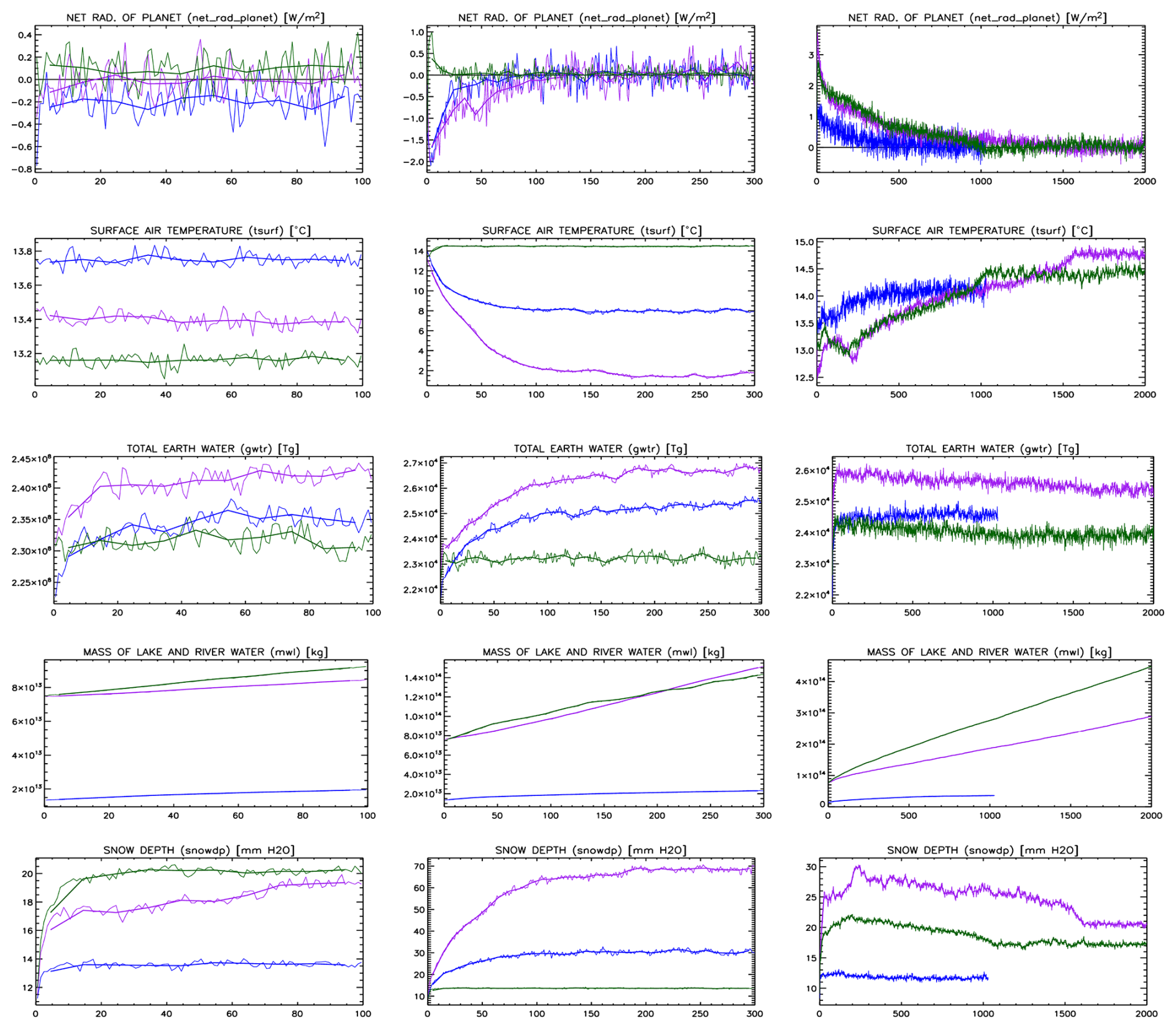
Figure 7Annual mean time series of net_rad_planet (first row), tsurf (second row), gwtr (third row), mwl (fourth row), and snowdp (last row) for the prescribed ocean simulations (left), the Q-flux = 0 ocean (middle), and the dynamic ocean (right) with SOCRATES and the x atmosphere. The ROCKE-3D 2.0 fine-resolution model is shown in blue, the ROCKE-3D 2.0 medium resolution is shown in purple, and the ROCKE-3D 1.0 medium resolution is shown in green. Note that the dynamic ocean simulation shown with a blue line in the last column equilibrated much faster than the other two, so only 1000 years are presented.
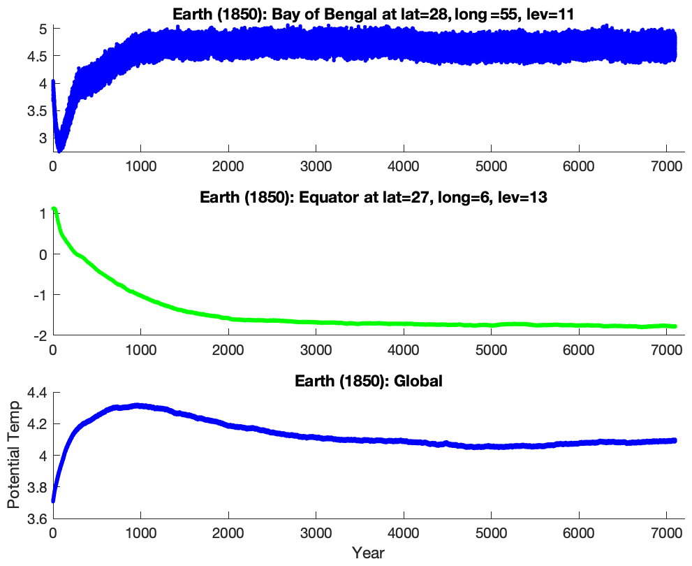
Figure 8Time series of ocean potential temperature (pot_temp) for a ROCKE-3D 1.0 simulation for modern Earth. The mean depth at level 11 is 1129 m and that at level 13 is 3868 m. Even after 1500 years it is obvious that neither the global mean nor the specific grid cells/levels appear to have leveled off. It was not until nearly 6000 years that the global ocean potential temperature began to level off. It is important to note that deeper oceans take longer to come into equilibrium.
The differences between ROCKE-3D 1.0 and ROCKE-3D 2.0 in the Q-flux ocean are due to the fact that the heat transfer used in ROCKE-3D 1.0 resembles that of Earth, so the initial conditions are much closer to equilibrium compared to Q-flux = 0 in ROCKE-3D 2.0. The dynamic ocean in ROCKE-3D 1.0 also equilibrates much faster, in about 1000 years, while the equivalent simulation in ROCKE-3D 2.0 needs over 1500 years. The fine-resolution model equilibrates much faster, in about 500 years. It is worth reiterating that here we are only referring to atmospheric radiative balance. If one has a deep dynamic ocean like that of modern Earth and one is interested in science questions related to such oceans, then it is vital to consider whether the ocean itself is in equilibrium. One way in which this can be explored is by looking at the mean global ocean potential temperature, but it is often useful to look at specific areas in the ocean as well as globally (Fig. 8).
4.3 Selecting the best template to start building a new world
Selecting the most appropriate model configuration for a simulation requires a careful balance of factors that affect both performance and results within the target science questions but also the appropriateness of the configuration for the planet of interest. A number of criteria need to be considered for making the best choice. The planet size can dictate the choice of resolution; for small planets like Mars the medium resolution is adequate, while for super-Earths the fine resolution might be more appropriate. Another factor to consider is whether the chosen resolution properly samples the Rossby radius of deformation, which depends on both the model resolution and the planet spin rate. The generally assumed notion that a higher resolution should always be preferred might not always be true (depending on the science question), because the computational cost of going from medium to fine is very significant (Sect. 4.5). In the case of exoplanets, for which we may have very few, if any, constraints on their atmosphere, there is often little point in performing fine-resolution simulations when the computational time might be better spent sampling over a larger parameter space with the medium resolution instead of gaining little additional scientific insight with a few high-resolution simulations.
For atmospheres that closely resemble that of present-day Earth the GISS radiation would suffice, so the simulation can take advantage of faster simulation times, while for very different atmospheres the SOCRATES radiation must be selected. If the planet has an ocean, the choice of a dynamic ocean configuration is always the best, while for a planet that closely resembles modern Earth the use of a prescribed ocean can be justified. For completely unknown planetary configurations the Q-flux ocean is a compromise between performance and oceanic response to climate, but the unknown factor of oceanic heat transport, presented later, can vastly affect (or bias) results. Lastly, the choice of atmospheric composition, both in terms of major and trace gases composition, is the parameter space that most ROCKE-3D users are expected to be routinely modifying. We do provide radiation tables for a wide range of compositions and stellar types (see “Data availability” section and Appendix C), but for cases outside the presently available tables the users would need to calculate their own. Any choice of planetary parameters (eccentricity, obliquity, etc.) should follow, since they do not affect the choice of the template used to initialize the model.
Another thing to consider when starting a new simulation is the spinup time required to bring the model to equilibrium. We provide equilibrated model conditions (restart files) for all simulations presented here (see “Data availability” section) or restart files that have been created previously can be used to spin off new simulations. The key thing to keep in mind is that the configuration changes between a restart file and a new simulation that the model code allows are limited. It is also important to note that restart files from ROCKE-3D 1.0 are not consistent with those of ROCKE-3D 2.0.
4.4 Creating a new planet
Although an infinite number of new planet configurations are in theory possible, in practice certain changes cannot easily be accommodated. Difficult changes include altering the horizontal resolution or vertical layering, incorporating a dynamic ocean when one was not used in prior simulations (although the reverse, starting a p or q ocean simulation from an o restart file, is possible), changing the land–ocean mask, topographic relief or ocean bathymetry while a simulation is ongoing, or altering atmospheric composition substantially. Altering the location of even a single land grid cell may require a series of cascading adjustments to many other boundary and initial condition data sets, which makes the task very tedious. It is not uncommon when whole-scale changes are made to continent and ocean configurations that fine adjustments must be made to deal with sub-grid-scale issues related to ocean gateways, vegetation distributions, or continental drainage basins (river flow and lakes). In this section we discuss some of the issues related to generating a new planet through the creation of self-consistent boundary and initial condition data sets. We also discuss a variety of pre-existing planetary and ancient Earth model configurations that are available for use with ROCKE-3D. A set of key parameters related to the definition of a new planet are presented in Table 4.
Table 4Description of parameters that are used to define a planet. Unless explicitly stated (footnote e) these parameters are modified via the model configuration “rundeck” file. NA: not applicable.
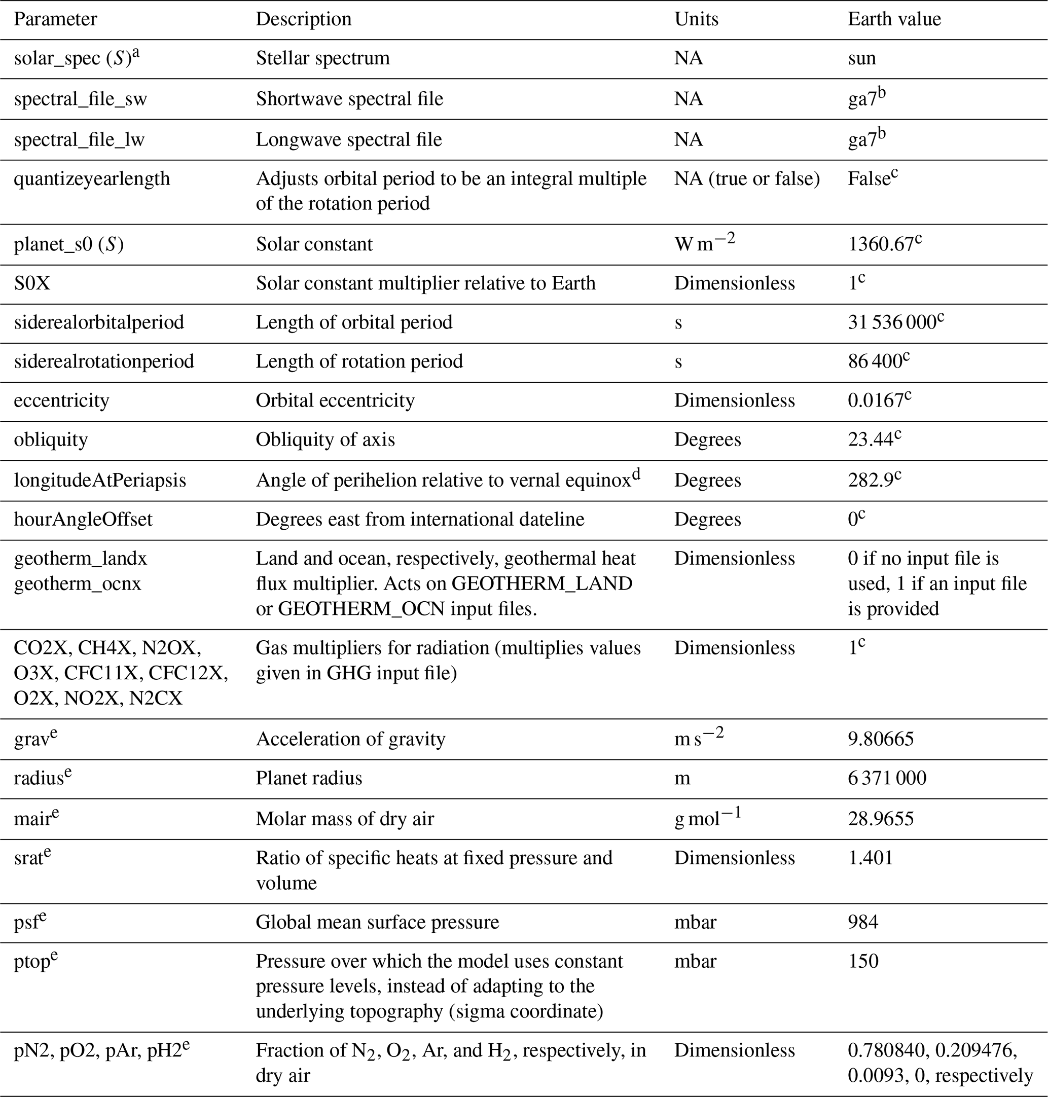
a Applicable only to the SOCRATES (S) or GISS (G) radiation scheme. b Multiple spectral files are permissible for Earth. sp_sw_ga7/sp_sw_ga7_dsa and sp_lw_ga7/sp_lw_ga7_dsa are used for the Earth runs presented in this paper, but these may be changed to allow for greater flexibility. c These default values do not need to be set explicitly for Earth runs. d This is sometimes called the “longitude of perigee” (see, e.g., Appendix B, Berger et al., 1993), which is 180° different from what they call the “longitude of perihelion”. In the GISS model, modern Earth's value is 282.9°. e Defined in the source code file shared/PlanetParams_mod.F90 rather than in the rundeck file.
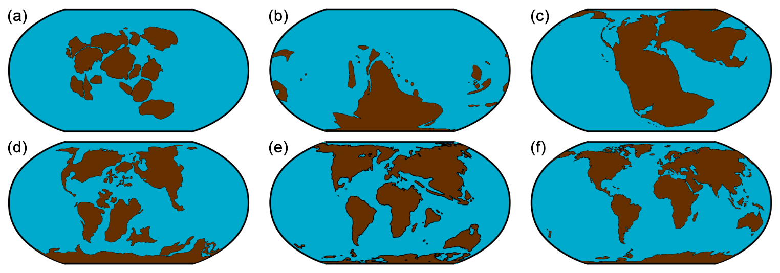
Figure 9Ancient Earth boundary conditions currently available. (a–c, left to right) Sturtian (Neoproterozoic Snowball Earth (720 Ma) and general Precambrian equatorial supercontinent configuration); Late Ordovician, 450 Ma; and Early Jurassic, 180 Ma (Pangaea supercontinent). (d–f, left to right) Mid-Cretaceous, 100 Ma; Cretaceous–Paleogene boundary, 66 Ma; and mid-Pliocene, 3 Ma.
4.4.1 Ancient Earths
A variety of boundary condition data sets (Fig. 9) that are based on paleogeographic reconstructions are available for use with ROCKE-3D. These ancient Earth boundary conditions represent various time periods throughout Earth's history. The specific configurations are not uniformly distributed in geologic time but were chosen to supply testable scenarios either for significant climatic events or because they represent noteworthy continent–ocean distributions that have potentially compelling impacts on the global or regional climate characteristics of a planet. The available boundary conditions (Fig. 9) include (1) the Sturtian (720 Ma), an equatorial supercontinent that is representative of the Neoproterozoic Earth and has primarily been used with Snowball Earth studies and examination of Earth's Cryogenian interval; (2) the Late Ordovician (450 Ma), with continents primarily located in the Southern Hemisphere, including a significant-sized land mass covering the South Pole, in contrast to the Northern Hemisphere, which is dominated by open ocean; (3) the Early Jurassic (180 Ma), a time period where the Pangaea supercontinent, the single supercontinent (and, consequently, a single large ocean as well), was roughly symmetrical about the Equator and nearly extended from pole to pole; (4) the Mid-Cretaceous (100 Ma), a period of long-lived extreme warmth, among the warmest intervals of the past billion years, and perhaps the closest Earth has gotten to a super-greenhouse climate since multi-cellular life forms evolved, during which the Pangaea supercontinent had broken up, with an early Atlantic Ocean allowing a flow of water across the Equator; (5) the Cretaceous–Paleogene boundary (66 Ma), which was the time corresponding to the Chicxulub asteroid impact event, thought to have contributed to the extinction of dinosaurs; and (6) the mid-Pliocene (3.2 Ma), during which continents were already approximately in their modern geographic locations but ice sheets were greatly reduced and consequently sea level was higher, altering global coastlines. The mid-Pliocene is thought to be the most recent period in Earth's history with global temperatures as warm as models predict for Earth's future, as a result of greenhouse gas increases. For much older time periods, where the preserved geologic record is too limited to reconstruct paleogeographic records that could be used to generate realistic boundary condition data sets, we generally use either the Sturtian supercontinent boundary conditions (described above) or an idealized continental configuration (see next section), or we simply run the model as a water world (aquaplanet) or land-only world.
With the exception of the mid-Pliocene reconstruction, which includes reconstructed bathymetry as outlined by Haywood et al. (2016), other maps of ancient Earth have a uniform ocean depth. This uniform depth is a simplification given that the details of ocean bathymetry are poorly known, if at all, further back in Earth's history. A reasonable depth for ancient Earth simulations is 3800 m; for Earth-like exoplanet simulations using these land distributions and a dynamic ocean, in the absence of any better constraint, we frequently use a depth of 1000 m.
4.4.2 Venus
All current versions of ROCKE-3D are unable to model modern-day Venus because of its extreme surface temperatures (∼750 K) and pressures (∼92 bar), but a number of studies of a hypothetically ancient habitable Venus have been published (Way et al., 2016; Way and Del Genio, 2020). In these studies five different sets of boundary conditions were utilized. Three of them involved the use of modern-day Venusian topography (can be found in Fig. 5 of Way and Del Genio, 2020): a land planet with only 20 cm of water incorporated within the soil (termed arid Venus), a planet with 10 m water global equivalent layer (GEL) called 10 m Venus with the water dispersed into the lowest topographic regions as dynamically active lakes (their existence/size determined by a competition between evaporation and precipitation during the model simulation), and a 310 m Venus with 310 m GEL again dispersed into the lowest topographic regions as oceans and lakes where the oceans are permanent features and the lakes again are dynamic. Two other cases were chosen as they are commonly used in the exoplanet literature: an aquaplanet scenario (with the only land being at the South Pole point and set to zero topographic height) and a modern Earth land–sea mask, but only using a 310 m deep ocean to make it comparable to the 310 m Venus scenario mentioned above. The reader would be right to ask why one uses modern Venusian topography when any ancient topography was likely completely different? First, it is an interesting contrast to modern Earth, which has a plethora of land at high latitudes, whereas the 310 m Venus has a lot of land also at low latitudes, in contrast to the aquaplanet scenario. Finally, with presently available data there is no way to reconstruct what ancient Venus' topography was like as ∼80 % of the planet has been resurfaced in the past ∼300–750 million years (Bougher et al., 1997; Strom et al., 1994). All boundary condition files for the cases described above are located in our online repository (see “Data availability”). In an attempt to compare some of the previously published ROCKE-3D 1.0 ancient Venus work with ROCKE-3D 2.0, we ran a number of ROCKE-3D 2.0 simulations with the exact same setup. Generally for the dryer simulations (arid Venus and 10 m Venus) the results were very similar (see Sect. 4.4.4 for Proxima Centauri b). For the simulations with oceans this was not always the case. For example, for the 310 m Venus case at 2.9 Ga ROCKE-3D 2.0 had a mean temperature of 3.4 °C, while the published ROCKE-3D 1.0 result (Way and Del Genio, 2020) was 9.6 °C. This difference of 6 °C is likely due to the very different cloud scheme differences between ModelE2.1 (ROCKE-3D 1.0) and ModelE2.2 (ROCKE-3D 2.0) as demonstrated in Fig. 10, where the planetary albedo and net cloud radiative effect are quite distinct.
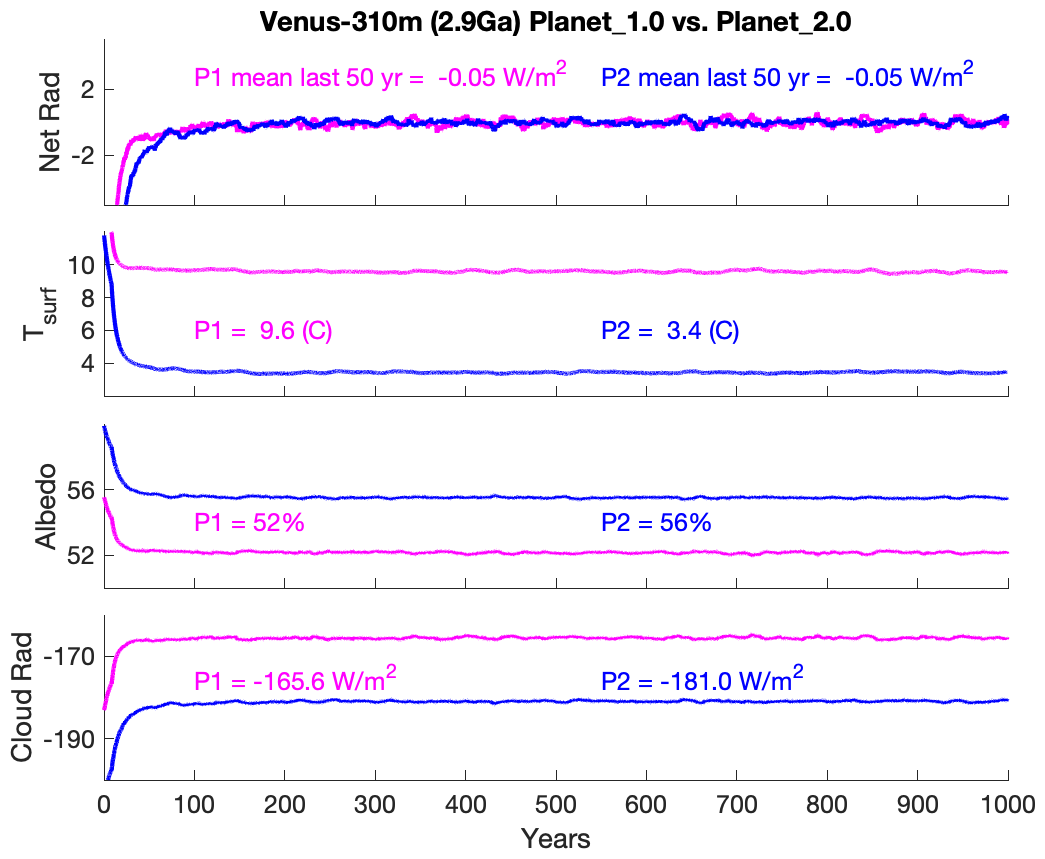
Figure 10Comparison of ROCKE-3D 1.0 and ROCKE-3D 2.0 simulations of an ancient Venus climate from simulation no. 25 in Way and Del Genio (2020). The simulation is of a 310 m deep global equivalent layer ocean that includes a number of low-latitude continents (Fig. 5 in Way and Del Genio, 2020). X axis: number of Venus orbits completed. Y axis: Net Rad – net radiative balance at the top of the atmosphere (net_rad_planet); Tsurf – global mean surface temperature (tsurf); Albedo – global mean planetary albedo (plan_alb); Cloud Rad – net cloud radiative effect (shortwave + longwave).
4.4.3 Mars and Moon
Mars has been modeled with ROCKE-3D for several epochs in its history, but thus far only ancient Mars simulations have been published. The simulations were aimed at the Noachian (Guzewich et al., 2021) and the Hesperian (Schmidt et al., 2022). In the Noachian case modern Mars topography was used (Guzewich et al., 2021), but a subset of simulations used a topography with an inferred map before the Tharsis region was formed, as well as its associated true polar wander (Bouley et al., 2016). In Schmidt et al. (2022) only modern Mars topography was considered. Guzewich et al. (2021) utilized varying amounts of GEL water, whereas Schmidt et al. (2022) only considered a northern polar ocean (∼10 % of the surface area of the planet) and the Hellas Basin to have water.
As part of its thin-atmosphere capability (see Sect. 2.2.3), ROCKE-3D is currently capable of simulating modern Mars with a pure CO2 atmosphere (∼6 mbar at surface) and fully coupled CO2, H2O, and dust cycles. For the water cycle it uses a three-layer snow model developed for the parent Earth model, while the CO2 condensation is currently handled by a bucket model which keeps track of the condensate amount and its areal cover fraction. The cover fractions of the H2O and the CO2 snow are combined together (the greater fraction absorbs the smaller fraction) for the computation of ground albedo. No distinction is currently made between CO2 and H2O snow in the albedo algorithm.
Soil dust aerosols have been incorporated into the Mars version of ROCKE-3D as radiatively active tracers by successfully utilizing the soil dust module that was developed for NASA GISS ModelE for Earth's atmospheric conditions, with only minor modifications. It is a sectional scheme with five size bins that simulates the emission, atmospheric transport, and deposition of dust. Different to the original scheme in ModelE, dust emission is explicitly dependent on atmospheric surface density (as a function both of pressure and temperature at the surface) to account for the large density variations at the surface of Mars, affecting the buoyancy of dust particles.
Following a hypothesis of Needham and Kring (2017) that in the past the Moon could have had a thin transient atmosphere due to volcanic outgassing, we used ROCKE-3D to study such an atmosphere (Aleinov et al., 2019). In our experiments, we used modern lunar topography and albedo, as well as conditions at ∼3.5 Ga (peak of lunar volcanic activity) for orbital parameters and insolation. A special algorithm was added to treat Permanently Shadowed Regions (PSRs) as patches of land which receive no shortwave radiation. We investigated a parameter space of surface pressures 1–10 mbar and compositions which included pure CO and pure CO2 atmospheres, either completely dry or with kg kg−1 water. The results have been presented in the past (Aleinov et al., 2019), and the configuration we provide can be used for similar model setups.
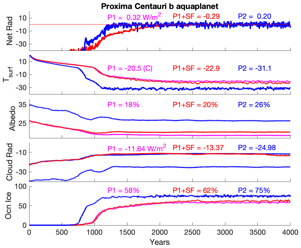
Figure 11Same as Fig. 10 but where P1 = ROCKE-3D 1.0 and P2 = ROCKE-3D 2.0. P1 + SF is the ROCKE-3D 1.0 version with the sea ice fix mentioned in Sect. 2.1. The bottom row is the fraction of the ocean covered in ice. Since this is an aquaplanet setup, that is equal to the planet surface covered in ice.
4.4.4 Known extrasolar terrestrial planets
The ROCKE-3D model has been used in a number of studies involving extrasolar planets and their theoretical atmospheres. For comparison purposes we examined results from Proxima Centauri b as an aquaplanet with a fully coupled ocean with ROCKE-3D 1.0 and ROCKE-3D 2.0. Here, it is important to note that there was an update to the sea ice parameterization from ROCKE-3D 1.0 to 2.0 as described in Sect. 2.1 above. Since the Proxima Centauri b control run from Del Genio et al. (2019b) is particularly cold, in order to make the comparison more realistic we did an additional control run with the ROCKE-3D 2.0 sea ice fix in ROCKE-3D 1.0. This can be seen in Fig. 11 below. As in the ancient Venus case discussed in Sect. 4.4.2 the clouds appear to play a key role in making the climate ∼8 °C colder in the ROCKE-3D 2.0 case versus in ROCKE-3D 1.0 with the sea ice fix (P1 + SF). Without the sea ice fix the difference is nearly 10.5 °C. This difference in the clouds manifests itself markedly in the amount of the ocean that is covered in ice as seen in Fig. 11. An additional 4 % of ice accumulates in ROCKE-3D 1.0 with the sea ice fix and another 13 % on top of that with ROCKE-3D 2.0.
ROCKE-3D participated in the THAI model intercomparison (Fauchez et al., 2020) that studied the planet Trappist-1e with the same boundary condition files and atmospheric compositions across four models (Fauchez et al., 2022; Sergeev et al., 2022; Turbet et al., 2022). Here we look at differences between ROCKE-3D 1.0 (used in the THAI intercomparison) for the dry case (Ben1) vs. ROCKE-3D 2.0 (Fig. 12). In this setup there is no moisture in the atmosphere or surface; hence there are no clouds. The planetary albedo is almost exactly the same, yet the surface temperatures still differ by ∼3 °C. This gives us a lower limit for the differences we can expect between the same setup on ROCKE-3D 1.0 vs. 2.0. In general, similar differences were seen in the dry cases in the THAI intercomparison (Turbet et al., 2022) and in related studies (e.g., Sergeev et al., 2024).
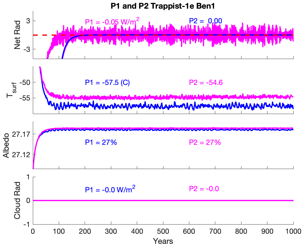
Idealized land–ocean configurations
Some studies focused on early Earth or terrestrial exoplanets will have experiment designs that require some representation of ocean and emergent land area but are not yet at a stage that would benefit from the complexities of the realistic ancient Earth boundary conditions described in Sect. 4.4.1. It may also be the case that the percentage of land area required is notably greater or less than the land coverage offered by those ancient Earth configurations (which range between 20 % and 30 % land cover). To fill this need, we have created sets of boundary condition files for 13 idealized continent configurations, in which land is represented at increasingly smaller fractions of the total global area (Fig. 13). Configurations with ≥25 % land cover are available in three orientations: pole-to-pole meridional, polar cap, and equatorial land belt. The smallest global land cover options, 12.5 % and 6.25 %, are each available as two- or four-continent distributions to emulate the presence of microcontinents. All 13 configurations have a uniform land elevation of 50 m, a ground albedo that is calculated by using a 50 % dark and 50 % bright soil mix, and include simple bathtub oceans, in which the seafloor slopes steeply downward from the continental edges to a uniform ocean bottom. The maximum depth is configurable and is typically set between 1000 and 3800 m for simulations with a dynamic ocean. Together with the two land planet and aquaplanet configurations, we cover a spectrum of land cover possibilities.
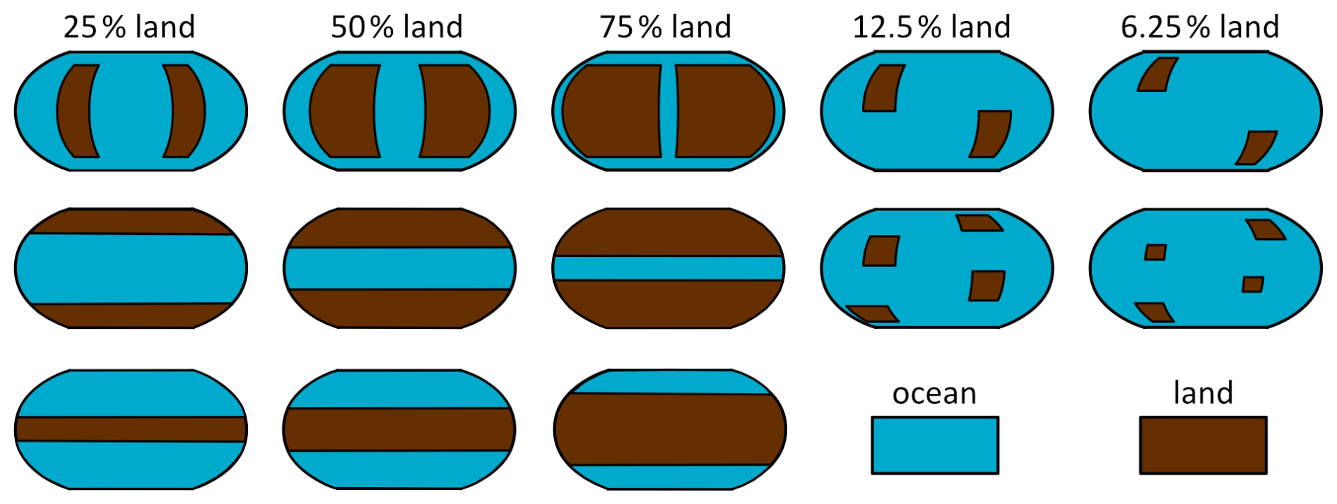
Figure 13Idealized continent configurations.
Aquaplanets
In addition to the Earth-centric configurations described here, we also provide four aquaplanet ones (GISS or SOCRATES radiation scheme, with dynamic or Q-flux = 0 oceans). Aquaplanets are commonly used configurations for studies in climate dynamics or for planets with unknown surface boundary conditions, as is the case for exoplanets.
The aquaplanets with a dynamic ocean are substantially warmer than the runs with Earth's topography (20.9 and 22.2 °C with SOCRATES or GISS radiation, respectively). They also feature a substantially reduced pole-to-Equator temperature gradient relative to Earth runs (Fig. 14) and a stronger greenhouse effect owing to the greater abundance of atmospheric water vapor.
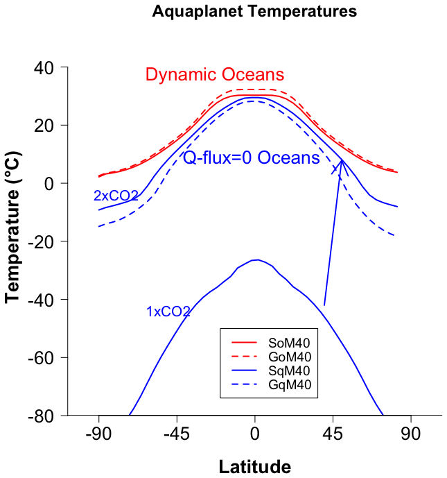
Figure 14Zonal mean temperature (°C) for aquaplanet simulations with the SOCRATES (solid) or GISS (dashed) radiation scheme and a dynamic ocean (red) or Q-flux = 0 ocean (blue) configuration. Two simulations (varying CO2 amount) are annotated for the SOCRATES Q-flux = 0 configuration, which exhibits a large change between 1×CO2 and 2×CO2.
The Q-flux = 0 aquaplanet runs are colder than their dynamic ocean counterparts and differ markedly between the GISS and SOCRATES radiation schemes (global mean temperature of 13.3 and −44.5 °C, respectively). This is due to a snowball (ice–albedo) instability that occurs for the SOCRATES but not the GISS run. Although this discrepancy is obviously large, we note that previous studies have shown that the coupling between sea ice and the convergence of ocean heat transport patterns is extraordinarily strong in aquaplanet simulations (e.g., Rose, 2015), and work in climate dynamics using aquaplanets often disables sea ice formation altogether due to the strong confounding influence of ocean heat transport on the stability of the sea ice edge (Rencurrel and Rose, 2018; e.g., Voigt et al., 2016). While sea ice is sometimes disabled in some aquaplanet studies to isolate specific dynamical processes, its inclusion is essential for fully coupled exoplanet simulations. Sea ice plays a critical role in setting the climate state, particularly in transitions between ice-free, waterbelt, and snowball regimes and tipping points, and strongly influences the planet's energy balance and climate stability (e.g., Brunetti et al., 2019; Hörner and Voigt, 2024). For the realistic exploration of exoplanet climates, especially near habitability boundaries, sea ice must be actively included. For the Q-flux = 0 aquaplanets, our simulations are very close to an instability threshold, such that simply changing the radiation scheme results in a large bifurcation despite only marginal differences in all other runs reported here. In fact, if the Q-flux = 0 aquaplanet simulation using SOCRATES is instead run (from initially warm conditions) with a doubling of atmospheric CO2, it does not transition into a snowball and is warmer than the GISS counterpart simulation with 1×CO2. The GISS radiation Q-flux = 0 aquaplanet run also collapses into a near-snowball state with 0.5×CO2, indicating that these simulations are quite sensitive near their current state. Such a CO2 forcing is a large perturbation in the context of contemporary climate change on Earth but is small by planetary climate standards. This is consistent with the studies discussed above in that aquaplanets are remarkably prone to large snowball instabilities and the Q-flux (or Q-flux = 0) configuration, in particular, should be used with caution for climates in which sea ice is expected to form.
4.5 Model performance
Model performance was discussed in the ROCKE-3D 1.0 paper (Way et al., 2017), but since its importance should not be underestimated, we further discuss it here. Each model component described here has its own computational requirements. The exact wall time for a simulation to complete does change depending on computer load (e.g., input/output contention) and hardware capabilities (e.g., CPU generation, memory availability), and it can fluctuate even from one simulation to the other on the same computer. For this, the values presented in Fig. 15 should only be used in a qualitative manner rather than as exact representations of the whole duration of a simulation on any computer at any given time. Even with these approximate numbers, it is clear that SOCRATES radiation is more computationally expensive than GISS, and the same applies for the fine resolution over the medium one. The prescribed and Q-flux ocean runs are practically indistinguishable when it comes to computation time, while the dynamic ocean is more computationally demanding. This difference is amplified with resolution: while moving from medium to fine resolution roughly increases the simulation time by a factor of 2–3, a direct result of the quadrupling of the atmospheric resolution, when the dynamic ocean is included the computational time increases by about an order of magnitude. This is an additive effect of the 4x atmospheric increase in resolution and the ∼40x oceanic increase (Table 1). Interestingly, the performance penalty added by the presence of a dynamic ocean in the medium resolution is overwhelmed by the slowdown due to SOCRATES, while for the fine resolution it is more pronounced. Further, the A atmosphere when using SOCRATES has a clear slowdown by about 50 %, probably linked with the presence of O3 and aerosol calculations that significantly add to the radiative transfer performance.
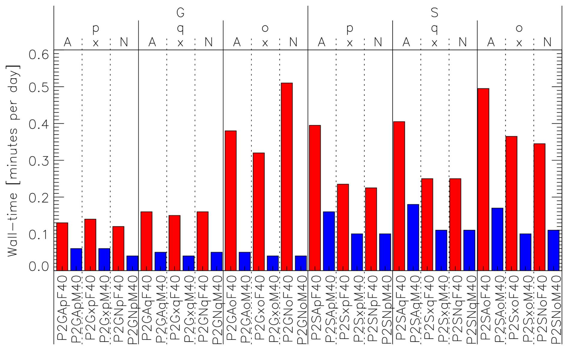
Figure 15Approximate wall time required per model configuration. The different atmospheres, oceans, and radiation schemes are listed at the top of the plot, while the two resolutions are separated by color (blue: medium; red: fine).
4.6 Further modifications of the model configuration
There are too many parameters that one can alter to modify the behavior of the model to list here. These involve either sanity-checking limits, expansion of capabilities, or fixes of known issues, as described in Sect. 4.6.1. In addition, during and after the end of the simulations presented here, model development continued. That led to some additional model development and bug fixes (Sect. 4.6.2) that are now available in ROCKE-3D 2.0 but were not available when the simulations presented here started. All the parameters below can be defined in the model “rundecks”, the configuration files that completely describe each simulation.
4.6.1 Parameters that can be modified
Beyond what has been presented thus far, there are several more ways one can modify how the model runs. These additional options can change physics (thus results), can significantly affect model performance, and/or can change what diagnostic output is produced. A comprehensive list and explanation of all options is far outside the scope of this work, so we only list here the most important, or most influential, of the parameters that ROCKE-3D users should be aware of. The key ones are described below, and many more are listed in Table 5.
Table 5Description of parameters that modify the model's behavior.
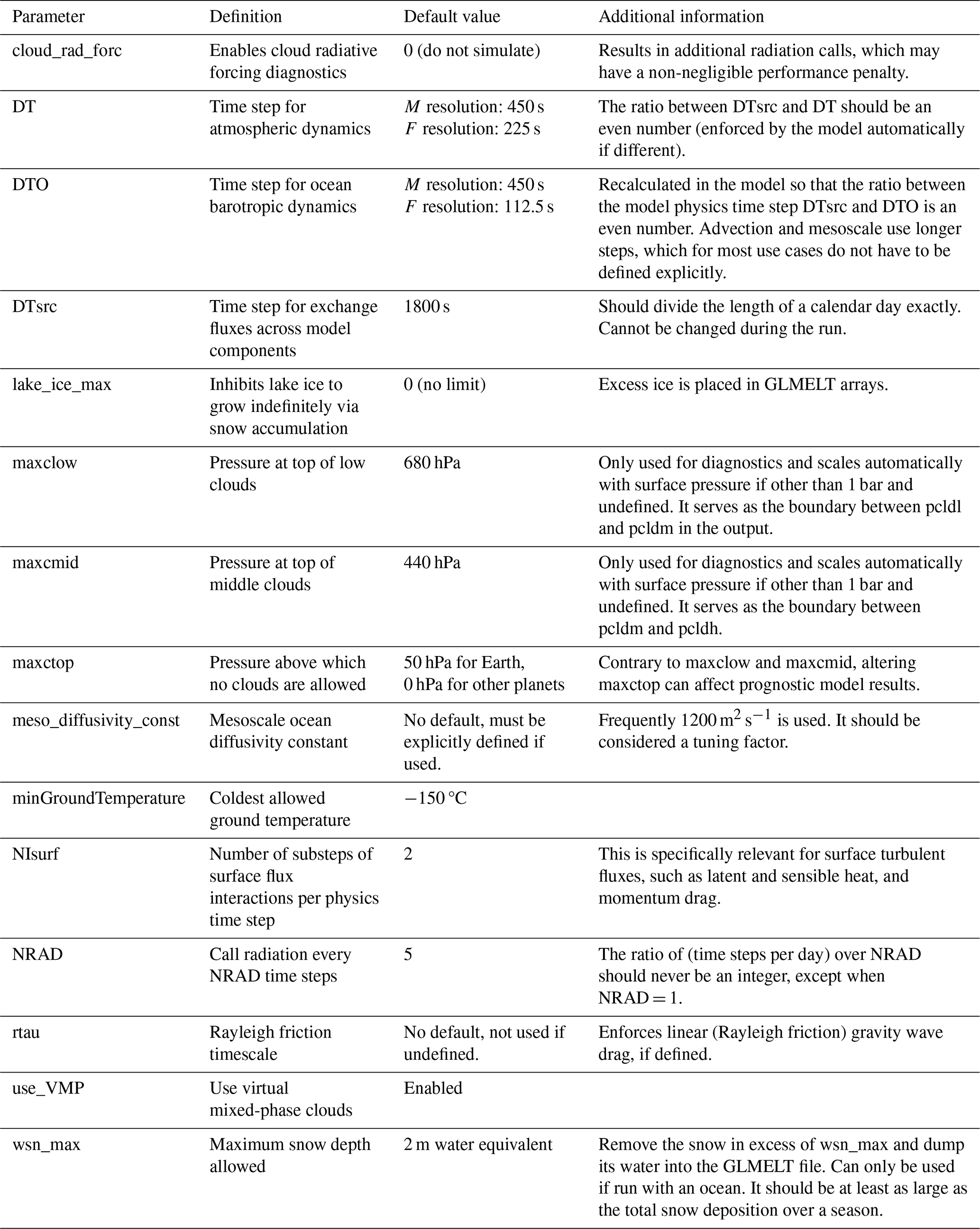
The main parameter which defines how the model is run is its physics time step, DTsrc. It tells the model how often its main parts (atmosphere, ocean, land, radiation) should exchange fluxes. Once set up at the start of a simulation, it cannot be changed. Other time-stepping parameters can be changed though, and we use this functionality if the model exhibits numerical instabilities during the course of a simulation. In particular, one can decrease DT or increase NIsurf (typically, by powers of 2) to improve stability. The choice of DT depends on many factors, but in general smaller planets and planets with thinner atmosphere need smaller DT. For example, for most of our modern Mars runs, we use DT = 50 s.
A key parameter related to both model results and model performance is NRAD, which stands for “every how many time steps radiation is called”. Ideally this should equal to 1 (every time step), but radiation is the most computationally expensive physics part of the model, so traditionally we use the value of 5. The choice of this value is not random: since the model is based on an Earth model, where the planet has a rotation period of 24 h, the default 30 min physics time step means that there are 48 time steps per day. The value of NRAD = 5 is the smallest non-unity value that does not divide 48 exactly, ensuring a non-uniform (thus, non-biased) sampling over the course of multiple days. In other words, over, e.g., a month, every 30 min period of the day is sampled, thus getting a non-biased average. For planetary applications, care must be taken for the choice of this variable: the number of time steps per day, which depends on the model time step and the rotation period, should never be exactly divided by NRAD, if NRAD > 1. Very large values of NRAD though will add a sampling bias, so the right balance between performance and accuracy needs to be maintained. Even beyond planetary rotation periods, for very fast rotators (e.g., orbital periods of very few days) one might not be able to use daily or “monthly” means if the choice of NRAD is such that radiation is called very few times over the averaging period.
4.6.2 Other updates and future developments
After the completion of the simulations presented in this paper, issues in the calculation of the ocean momentum diffusion terms were discovered in ROCKE-3D 2.0 and were fixed. These include (1) some quantities used in the tridiagonal solver for the ocean velocities that were not defined properly and (2) the hemispheric symmetry that was re-established in the calculation of some intermediary arrays. The impact of these bug fixes was evaluated in the framework of ModelE2.1 at preindustrial (year 1850) conditions, and these bug fixes were found to have a minimal impact on the global climatology. They are nonetheless necessary to have full ocean dynamic hemispheric symmetry for aquaplanet runs and are now enabled by default in ROCKE-3D without user intervention.
Deep ocean worlds
In order to explore a wider range of planets and moons with deep oceans (on the order of tens to hundreds of kilometers deep), an upcoming update to ROCKE-3D 2.0 will extend the ocean component from a hydrostatic (H) model to a quasi-hydrostatic (QH) model. With an increasing number of planets presumed to have surface oceans or icy moons with subsurface oceans (e.g., Europa, Enceladus), some assumptions made about the H momentum equations for planets with relatively shallow oceans like Earth (, where h is the ocean depth and R is the radius of the planet) need to be revisited to take into account (1) planetary bodies with ocean depths reaching tens of kilometers and (2) cases where ocean depths are not negligible anymore when compared with the planet or moon radius (Marshall et al., 1997). Hydrostatic primitive equations (HPEs) were developed as a less GCM computationally expensive form of the full non-hydrostatic (NH) momentum equations by considering Earth's oceans in a hydrostatic balance where the pressure field is balanced by the gravity force. In cases where is not small anymore (e.g., for Enceladus) the QH setup is considered to be more realistic for deep oceans than the H equations, while not being as computationally expensive as the NH ones. This is achieved by re-establishing some of the Coriolis and metric terms neglected in the momentum equations to get a full treatment of the Coriolis force and by relaxing the shallow water approximation in the momentum equations. As an example, in spherical coordinates where r was constant and equal to R, the vertical position of a parcel of water r is now a variable. When this update is finalized, it will be made available as an easy-to-implement update into ROCKE-3D 2.0.
The effects of the different model configurations presented in Table 1 on the modeled climatology are presented below, together with other configurations that are available in ROCKE-3D 2.0 but are not based on Earth. We present the latter ones as means to compare the results of ROCKE-3D 1.0 simulations using ROCKE-3D 2.0. We expect that the most popular configuration will include the SOCRATES radiation (S), using an anoxic atmosphere (N), a dynamic ocean (o), and the medium resolution of the model (M40), so P2SNoM40. When studying differences across configurations below, we will use that simulation as the point of reference, to the extent possible.
5.1 Quick view
The results across simulations present large differences that show the impact of configuration choices on the overall climate of the atmosphere in question. We will first take a quick look at the global mean results (Fig. 16), before diving deeper into regional changes in subsequent sections. The first thing one notices when comparing Fig. 5 with Fig. 16 is how much more colorful the latter is, implying that the simulated differences across planetary configurations are much more impactful to climate variables than the changes we did towards the generalization of the Earth configuration. In other words, the climatological differences we get when simulating Earth with and without any Earth-centric tunings are much smaller than the differences seen when simulating different planets. This provides an additional assurance that the generalization procedure does not negatively impact model skill.
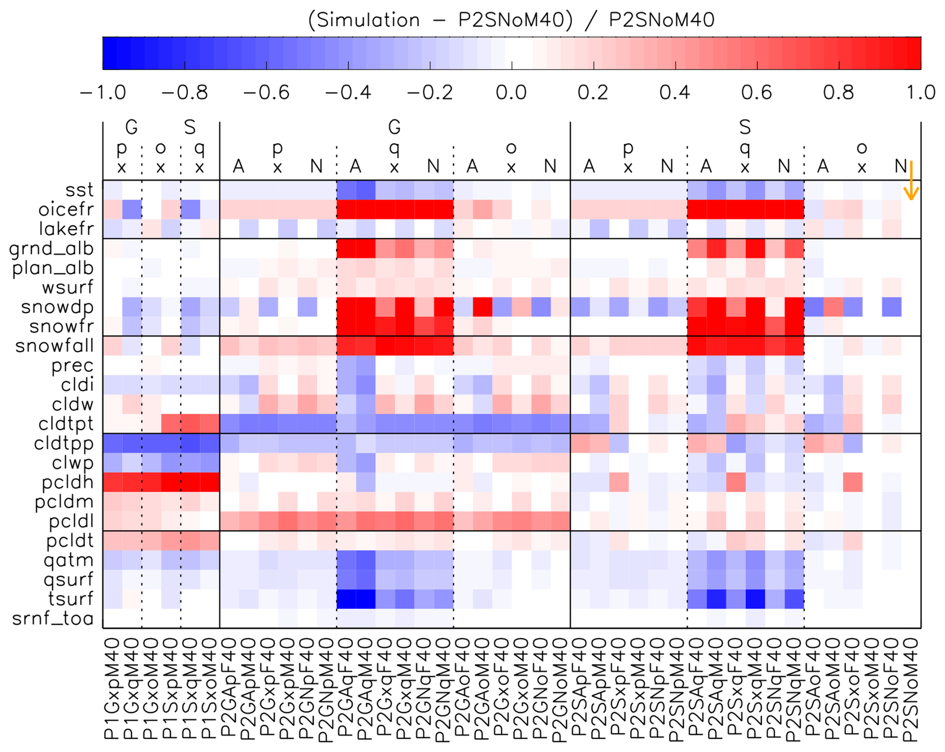
Figure 16Same as in Fig. 5 but for the template configurations described in Table 1. Note the addition of a legend over the plot, which makes understanding the differences across columns easier. Also note that contrary to Fig. 5, all simulations presented here are in radiative balance.
Starting from comparing the old (Way et al., 2017) against the new (this work) ROCKE-3D versions, the biggest changes are found in the high cloud fraction (pcldh), which drops from 58 % in ROCKE-3D 1.0 to 29 % in ROCKE-3D 2.0 when averaging across all simulations – a value much closer to the value expected for present-day Earth. Together with some modest middle- and low-level cloudiness, the mean total cloud fraction (pcldt) for all simulations decreased from 75 % in ROCKE-3D 1.0 to 59 % in ROCKE-3D 2.0. The cloud top pressure in ROCKE-3D 1.0 is lower than in ROCKE-3D 2.0, which means that clouds were able to reach higher altitudes in the previous version of ROCKE-3D.
When looking at the ROCKE-3D 2.0 results and comparing them with P2SNoM40, two major patterns appear. One is related to clouds and radiation: when averaging out over simulations that use the GISS radiation, low cloud fraction (pcldl) is 44 %, compared to when averaging over SOCRATES simulations where it is 32 %. This is an expected difference that results from the U00b cloud balancing values we used (Table 3), which are higher in all GISS simulations: larger U00b values reduce the critical relative humidity for cloud formation, making it easier to form clouds in grid cells where the U00b scheme is used. Another difference is that with the GISS radiation the tropopause temperature (ttrop) and pressure (ptrop) are both consistently lower than the reference simulation (P2SNoM40), while in the simulations using SOCRATES radiation there is no consistent pattern, with both positive and negative changes. ROCKE-3D uses the definition by the World Meteorological Organization (WMO) to calculate the tropopause layer, as the lowest level at which the temperature lapse rate decreases to 2 K km−1 or less.
Another major pattern that appears in Fig. 16 is the large changes calculated by the Q-flux = 0 ocean simulations. As will be detailed in Sect. 5.4, the absence of heat transport via the ocean makes the ocean much colder, resulting in colder sst, increased ocean ice fraction (oicefr) and ground albedo (grnd_alb), and increases in all snow metrics. Surface air temperature (tsurf) also drops when using the Q-flux = 0 ocean configuration, which results in less water vapor at the surface (qsurf) and in the column (qatm). This is a robust response regardless of the choice of radiation scheme, atmospheric composition, and resolution, although the magnitude of the effect does change across simulations.
5.2 GISS vs. SOCRATES radiation schemes
ModelE uses the GISS radiation scheme by default; with everything else held constant but switching radiation from GISS to SOCRATES (ga7_dsa spectral file), the model calculates a net planetary radiation imbalance of about −1.3 W m−2 when prescribed sst is used for the A atmosphere. An imbalance is expected for such simulations, where physics changes happen in the atmosphere but the ocean is not allowed to respond. The balanced SOCRATES simulation with a dynamic ocean produces small differences in the global mean climatology of surface air temperature (Fig. 17) but has some significant regional differences (Fig. 18). Interestingly, the GISS radiation simulates cooler temperatures at high latitudes compared to SOCRATES when the A atmosphere is used, with the exception of the region over the North Atlantic, where a strong heating is calculated. This heating negatively correlates with less cloudiness, so more sunlight penetrates to the surface, and a complete disappearance of sea ice from the region.
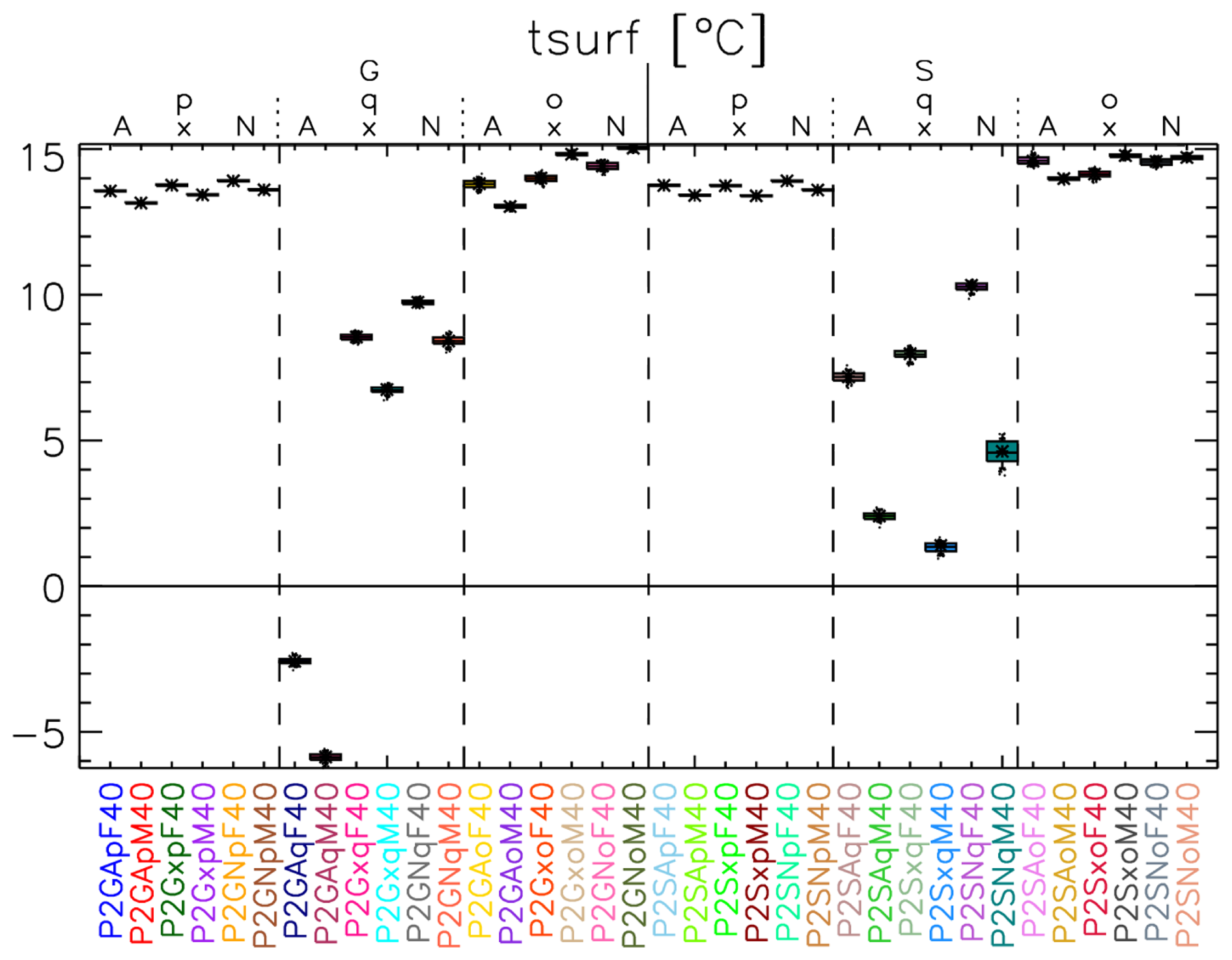
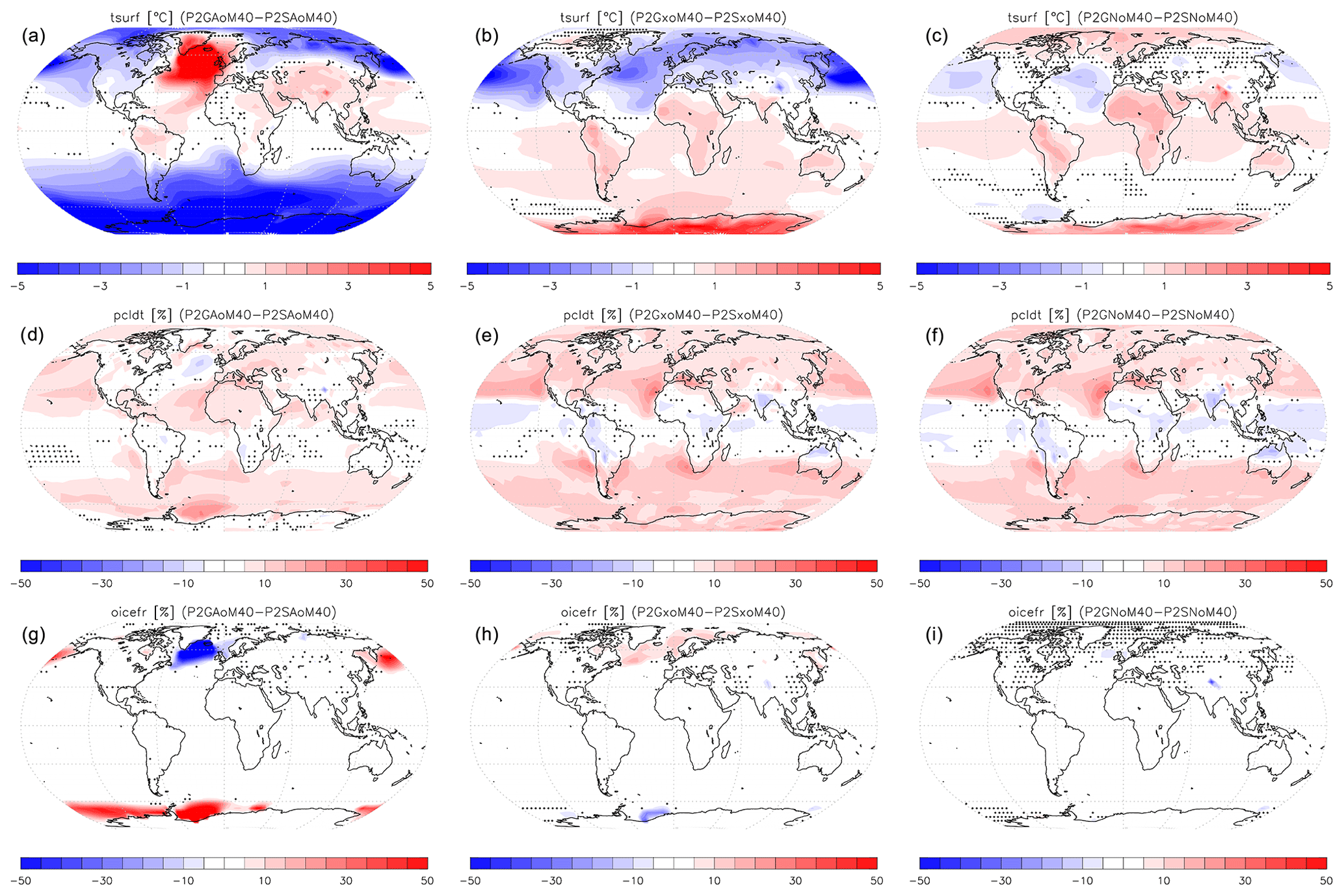
Figure 18Surface air temperature (a–c), total cloud cover (d–f), and ocean ice fraction (g–i) differences between GISS and SOCRATES radiation simulations for the A (a, d, g), x (b, e, h), and N atmospheres (c, f, i) with a dynamic ocean. Positive values mean the GISS radiation is warmer, and black dots show areas where the differences are not statistically significant at the 95 % confidence level.
The behavior observed in the A-atmosphere configuration appears to stem from the absence of an active overturning circulation in the SOCRATES radiation scheme case for the M resolution, which effectively shuts down the northward transport of heat. In contrast, the simulation using the GISS radiation scheme maintains a robust Atlantic Meridional Overturning Circulation (AMOC) of approximately 23 Sv, accounting for the warmer temperatures over the North Atlantic and the associated reduction in sea ice area relative to the SOCRATES run. While the radiation scheme does not directly control ocean circulation, its influence on surface energy fluxes may indirectly affect AMOC stability. In our model, AMOC strength has been shown to be highly sensitive to freshwater input from ice melt and transport (Romanou et al., 2023), suggesting a possible link. We also note that at the higher F resolution, both the SOCRATES and GISS simulations exhibit an active AMOC.
The x and N atmospheres on the other hand behave differently when the radiation scheme changes: the Southern Hemisphere mostly heats up and the Northern midlatitudes cool, while the North Pole heats up when using the N atmosphere (cools when using x). Sea ice changes again anti-correlate with surface air temperature, while clouds respond in a very similar manner between the x and N atmospheres, with a reduction over the tropical belt and an increase everywhere else, and in particular over the upwelling midlatitudes in both hemispheres. This shows the different response of GISS radiation with regard to aerosols and stratospheric O3, which are the main differences of the A atmosphere with x and N, but also to clouds, due to the different cloud balancing values selected (Table 3) which produce more low clouds (U00b) and total (U00a and U00b) with the GISS radiation choice of values. In the x simulations (central column in Fig. 18), the Southern Hemisphere becomes warmer with the GISS radiation and features increased cloud cover. However, the Northern Hemisphere becomes colder, also with more clouds. This particular GISS–SOCRATES difference appears to be the superposition of two other GISS–SOCRATES differences: one, the model wants to be cooler at high latitudes with the GISS radiation, excepting the North Atlantic AMOC-related feature, and two, the model wants to be warmer at southern high latitudes when using the GISS radiation (and slightly warmer at northern high latitudes) and when changing the atmospheric composition (and cloud tuning) but holding the ocean circulation fixed. When we combine these two patterns, we get the Southern Hemisphere warming in Fig. 19 slightly winning out over its cooling in the upper left of Fig. 18, but in the Northern Hemisphere the Fig. 18 cooling wins over the Fig. 19 warming.
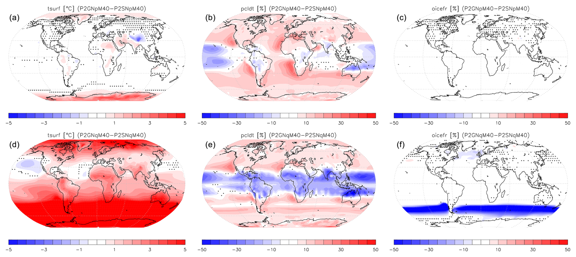
Figure 19Surface air temperature (a, d), total cloud cover (b, e), and ocean ice fraction (c, f) differences between GISS and SOCRATES radiation simulations for the p (a–c) and q (d–f) oceans with the N atmosphere; see Fig. 18 for the o ocean. Positive values mean the GISS radiation is warmer, and black dots show areas where the differences are not statistically significant at the 95 % confidence level.
Focusing on the N atmosphere (Fig. 19), the change in radiation scheme using a dynamic ocean resembles that of the prescribed ocean surprisingly well, with two notable differences: the continental warming is more pronounced and extends to the whole tropical belt, although in a smaller magnitude over tropical oceans, and there is a persistent cooling over the northern midlatitude oceans. All of those changes are too small, less than 5° everywhere, when compared to the differences between the two Q-flux = 0 simulations, in which major temperature differences are calculated between the two radiation schemes. GISS radiation calculates a very widespread warming over the polar half of the Southern Hemisphere, which exceeds 10 °C nearly everywhere and reaches 18 °C locally. This is consistent with a much less extended sea ice cover in the Southern Hemisphere when using the GISS radiation, which moves the Southern Hemisphere ice line about 10° further away from the tropics (Sect. 5.4). The clouds respond in a similar way across ocean configurations when the radiation scheme changes, with the GISS radiation leading to less clouds in the tropics and more in the extratropics. The differences in cloud cover between the GISS and SOCRATES simulations are generally consistent with the differences in the cloud tuning parameters, at least in the extratropics where there are the most stratiform clouds (the tuning parameters are for stratiform clouds). In particular, the A-to-x changes to those parameters for the GISS radiation are very large compared to typical changes for rebalancing Earth and go in the direction of making Gx a cloudier world. Interestingly, the SOCRATES radiation did not require such a large change for A-to-x rebalancing, perhaps because its radiusl_multiplier was left unchanged, while the A-to-x rebalancing for the G radiation increased radiusl_multiplier, which tends to make clouds less opaque and thus requires increases in cloud cover to compensate (decreased U00a, increased U00b).
The vertical profile of the global mean temperature (Fig. 20) for the different atmospheres used shows the major changes in the stratosphere that occur for the x and N atmospheres, a direct result of the absence of stratospheric O3. The absence of a stratospheric temperature inversion has important implications on several metrics of the model, as presented here and in other sections. Only the dynamic ocean and medium resolution is shown in Fig. 20, but the results discussed here are valid for all ocean configurations for both resolutions. For the preindustrial atmosphere (A), both the GISS and SOCRATES radiations agree very well, while all other atmospheres agree with each other in the troposphere only. Starting from the lower stratosphere, at around 50 hPa and higher, temperatures start to deviate with altitude and reach 10 °C at the model top, across radiation configurations. The x and N atmospheres with SOCRATES are virtually identical, which indicates that the GISS radiation might consider O2 and Ar (both absent in the anoxic (N) atmosphere) differently than SOCRATES does. Further, the GISS radiation simulates a very weak inversion that maximizes around 10 hPa, which is not calculated by SOCRATES, with implications for water vapor and high-altitude clouds. The ROCKE-3D 1.0 configuration, only available for the x atmosphere and medium resolution, agrees extremely well with its successor (P2SxoM40) in ROCKE-3D 2.0, except in the region between 100–10 hPa, which shows a much smoother transition in specific humidity rather than the sharper change in slope with altitude in ROCKE-3D 2.0 at around 50 hPa.
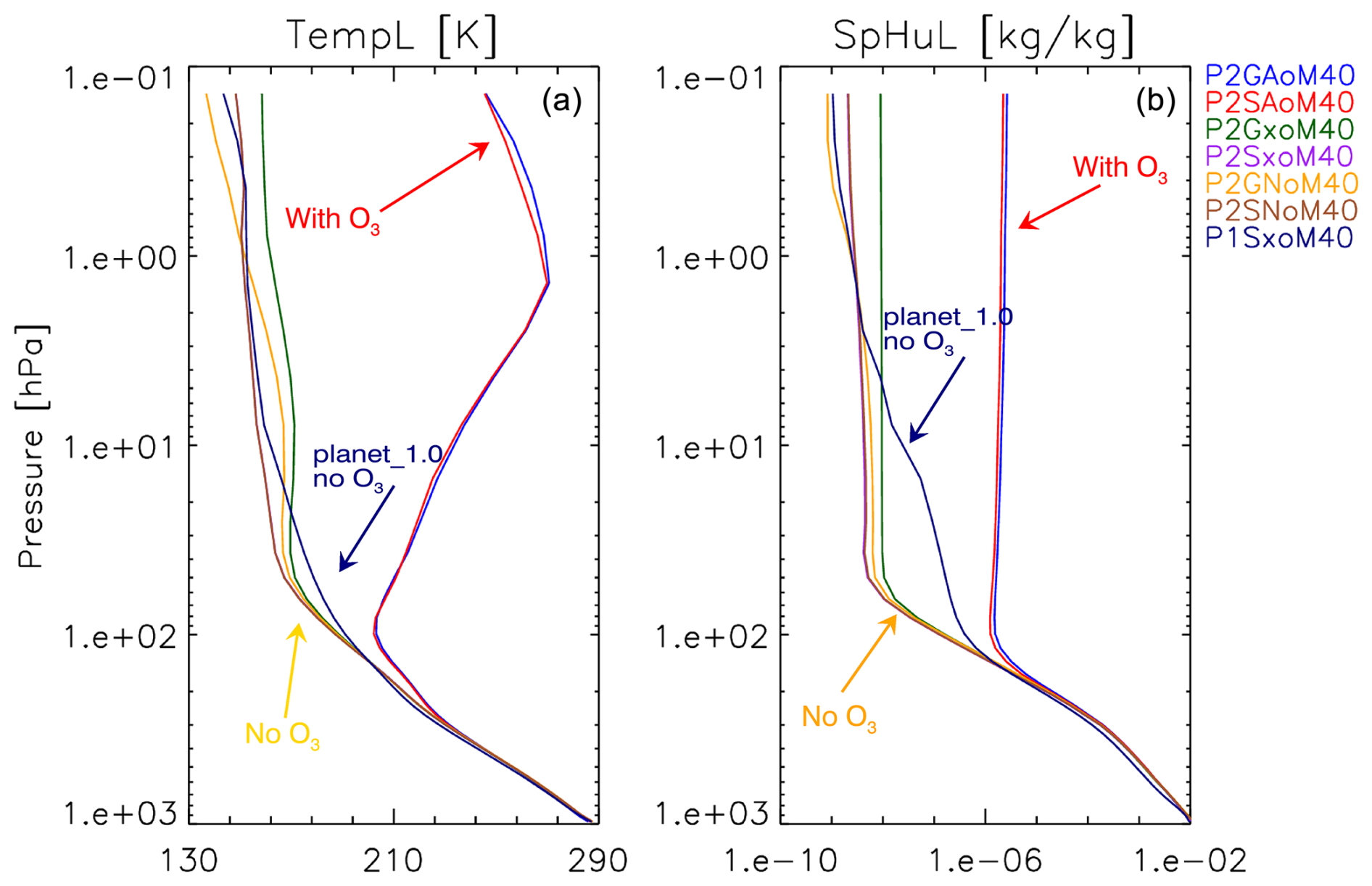
Figure 20Global mean temperature (TempL; a) and specific humidity (SpHuL; b) vertical profile using the dynamic ocean configuration for the different atmospheres and radiation schemes. The vertical profile calculated for the SxoM40 configuration from ROCKE-3D 1.0 is also included for comparison.
5.3 Earth vs. ROCKE-3D 1.0 vs. anoxic atmospheres
The removal of aerosols and O3 (and H2O from CH4 oxidation in the stratosphere to a lesser extent) in the ROCKE-3D 1.0 atmosphere has a very strong impact on the modeled climatology. First and foremost, the vertical temperature profile of both atmospheres without O3 (x and N) does not create a stratospheric temperature inversion, leading to large changes in the vertical temperature profile (Fig. 20), water vapor amount, and the presence of clouds (Fig. 21). The specific humidity (water vapor concentration) is nearly identical across configurations in the troposphere but deviates in the stratosphere due to the temperature differences simulated. The A atmosphere maintains a near-constant profile in the stratosphere with concentrations of around 2 ppmm (parts per million by mass; mg H2O kg−1 of dry air), while the x and N atmospheres have 2 to 3 orders of magnitude lower concentrations. This is directly explained by the much colder temperatures in the x and N atmospheres at the altitudes where the stratosphere exists in the A atmosphere, which makes it unable to hold a lot of water vapor, despite the absence of the cold trap in the tropopause. In ROCKE-3D 2.0 the transition from a decreasing concentration with altitude in the lower atmosphere transitions very quickly to a near-constant profile higher up, while in ROCKE-3D 1.0 there was a much more gradual decrease, driven by the temperature profile (Fig. 20).
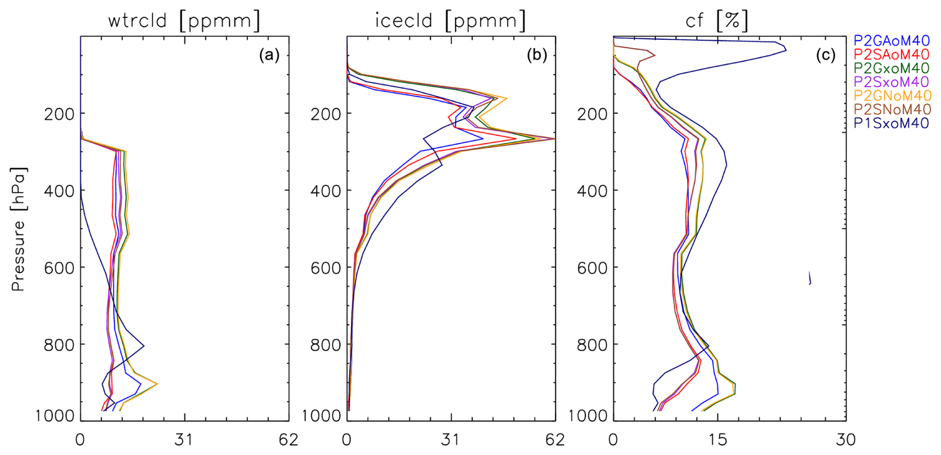
Figure 21Global mean concentration (in parts per million by mass) of water clouds (a), ice clouds (b), and total cloud fraction (c) vertical profiles using the dynamic ocean configuration for the different atmospheres and radiation schemes. The vertical profile calculated for the SxoM40 configuration from ROCKE-3D 1.0 is also included for comparison.
The vertical distribution of clouds also changes depending on the configuration. In ROCKE-3D 1.0, liquid water clouds are virtually absent above 400 hPa (Fig. 21), while in ROCKE-3D 2.0 there is a persistent liquid cloud presence throughout the column, until the temperatures become too cold and water clouds abruptly give way to ice. This happens because in ROCKE-3D 2.0 it is possible to form supercooled liquid clouds via a new virtual mixed-phase (VMP) cloud parameterization (Kelley et al., 2020), which was not present in ROCKE-3D 1.0 and significantly increases the amount of supercooled water cloud in the Southern Ocean and the Arctic. This parameterization is enabled by default in ROCKE-3D 2.0, but it is optional and can be disabled (Appendix B), although rebalancing of the model would be required in that case. Near the surface, the radiation scheme choice appears to impact low clouds, with the simulations using the GISS radiation calculating more clouds than those with SOCRATES, but this is due to different model balancing choices across radiation configurations (Table 3), not due to radiation scheme itself. Ice clouds are very similar between the two ROCKE-3D model versions (Fig. 21).
5.4 Prescribed vs. Q-flux vs. dynamic oceans
The simulations with the prescribed ocean have the smallest changes in surface air temperature when other model configurations change, in particular over the ocean (see, e.g., top-left panel of Fig. 19 for the p ocean vs. the bottom-left panel of the same figure for the q ocean vs. the top-left panel of Fig. 18 for the o ocean, when looking at the changes due to the radiation scheme selection; other panels in those two figures present additional variables). This is because the air–sea heat exchange over the ocean is driven by sst, which is constant across configurations, and the atmospheric forcing induced by the different configurations and the different balancing parameters is not strong enough to change surface air temperature a lot, in particular when it comes to global mean temperature. This is, however, not the case for the Q-flux = 0 and dynamic ocean configurations, in which the ocean, including its surface temperature, is allowed to respond.
When ocean configurations change across simulations, large differences are calculated in the model results. In the Q-flux = 0 case, differences are expected to be large by design due to the zero heat flux assumed, which is clearly different from the heat transport that is implicitly included in the p and o oceans. In the Q-flux = 0 case any horizontal heat transport can only occur via the atmosphere. All Q-flux = 0 model configurations extend the polar ice caps further away from the poles, in agreement with past studies (e.g., Seager et al., 2002; Winton, 2003), by as much as 16° when compared to the prescribed ocean and 32° when compared to the dynamic ocean, which is more pronounced when the SOCRATES radiation is used (Fig. 22). The more extensive ice caps are a direct result of heat that is mostly deposited near the tropics on Earth (due to its obliquity) and is not able to move fast enough towards the poles via the ocean, resulting in much colder extratropics and poles, which favor the extended ocean freezing. This effect is expected to be amplified on fast-rotating planetary configurations with obliquities lower than that of Earth (23.44°), including the typical value of zero used in the literature. It has to be remembered that in ROCKE-3D 1.0 the Q-flux ocean was using modern Earth's horizontal heat transport instead of zero, resulting in simulations that resemble more the p and o oceans. Since this has limited applicability in a generalized model where even the slightest change in continental configuration or bathymetry would make such a setup invalid, we decided to use the more easily manageable and more popular configuration (e.g., Batra and Olson, 2024; Sergeev et al., 2022; Wolf et al., 2022) of zero heat transport, although it is highly likely that it will not be the optimal choice for any planet.
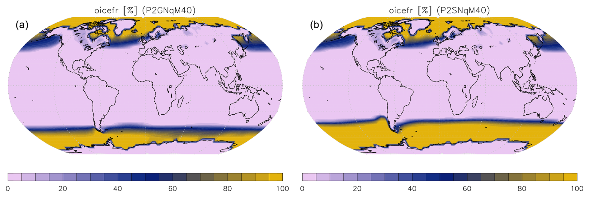
Figure 22Sea ice cover for the Q-flux = 0 ocean configuration when the GISS (a) and SOCRATES (b) radiation is used. Global means are 13.5 % for GISS and 19.2 % for SOCRATES.
The global mean ocean ice fraction (oicefr, which includes lake ice) is much higher in all Q-flux = 0 ocean simulations than the prescribed ocean that uses climatological sea ice cover from the preindustrial period, while the dynamic ocean oicefr is similar to that of the prescribed ocean (Fig. 23). For the Q-flux = 0 case the Earth's atmospheric composition with the GISS radiation has much more ice than any other simulation – a direct result of the lower temperatures simulated, which are globally averaged below freezing (Fig. 17).
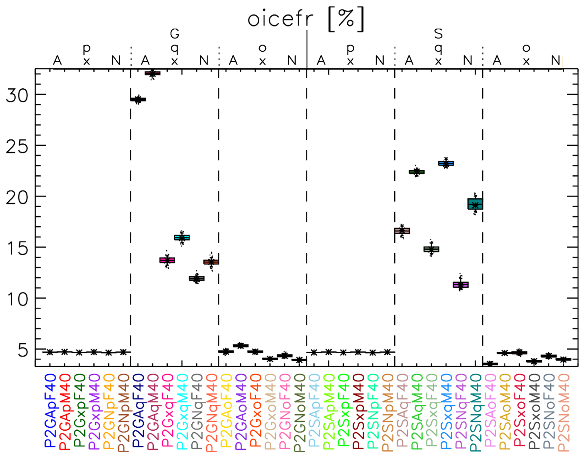
As mentioned earlier, the model-simulated tsurf resembles the underlying sst, regardless of the ocean parameterization used. For the p ocean the difference between the A and N atmospheres for sst is zero (they both use the same input data), and for tsurf the differences are very small, in particular between 60° S and 60° N latitudes, and maximizes at 2 °C near the North Pole (blue vs. green lines in Fig. 24). The fact that for the same sst there are differences in tsurf means that the A-atmosphere simulation tries to calculate cooler polar temperatures, which is evident when comparing the two o ocean simulations (red line in Fig. 24 vs. zero, since P2SNoM40 is the control). P2SAoM40 is colder at both poles, by as much as 7 °C at the North Pole, which contributes to the buildup of much more sea ice than the p oceans, resulting in cooler sst. It is worth mentioning that for sst the difference between all simulations presented in Fig. 24 is practically zero below sea ice at the North Pole, which demonstrates that ice insulates the underlying ocean from the atmosphere above.
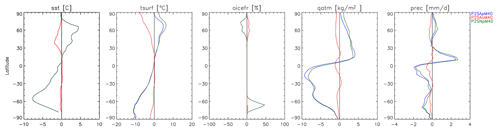
Figure 24Zonal mean difference from P2SNoM40 for sea surface temperature (sst; first panel), surface air temperature (tsurf; second panel), ocean and lake ice fraction (oicefr; third panel), total atmospheric water vapor load (qatm; fourth panel), and total precipitation (prec; last panel).
Another thing worth mentioning is the presence of water vapor in the atmosphere, which is greater in the Northern Hemisphere for the p oceans and lesser in the Southern Hemisphere, following tsurf. What is also interesting is that the tropical precipitation is further north for the p oceans compared against the dynamic ocean simulations, which means that the Intertropical Convergence Zone (ITCZ; the meteorological Equator) shifts northward when the temperatures are warmer there.
5.5 Medium vs. fine resolutions
The change in resolution, although technical in nature, introduces some important changes in the results. As a reminder, the resolution change is not the same in the atmosphere and in the ocean: in the atmosphere the 4°×5° latitude by longitude M resolution doubles to 2°×2.5° in F, with the vertical layering remaining the same, while for the ocean the resolution increases by an order of magnitude, going from 4°×5° and 13 vertical layers to 1°×1.125° and 40 layers. The ocean change is particularly important since the F resolution better resolves the coastline and narrow straits, as well as the different bathymetries across the global ocean. Vertical mixing is an important process sustaining the oceans' overturning circulations (Munk and Wunsch, 1998; Wunsch and Ferrari, 2004). For Earth simulations, the circumstances generating this mixing (vertical shear and negative buoyancy stratification) occur less frequently in the model at coarse resolution, and the circulation response to the mixing is also muted. The lack of semi-prescribed tidally induced vertical mixing in these simulations also pushes them toward weaker overturning. To avoid shutdowns of the Atlantic overturning circulation in the M configurations, we increased the condition-independent background vertical diffusion from 0.1 to 0.6 cm2 s−1.
An important result when comparing model resolutions is that all M runs with the p and q oceans are colder (Fig. 17). The difference in surface air temperature is very small in the p ocean configuration, since tsurf is still driven by the prescribed sst, which is the same across simulations, but interpolated on a different grid. The differences are also very small compared to other pairs of simulations discussed in the previous sections. For the q ocean though, the change from M to F resolution results in a strong global mean surface warming across model configurations, about 2 °C for GISS and almost 6 °C for SOCRATES, compared to the marginal increase for the p ocean.
The different resolutions also lead to a change in the north–south gradient of sst across all dynamic ocean configurations (Fig. 25). The fine-resolution simulations result in warmer temperatures across all northern midlatitudes, with zonal mean values reaching 6 °C, while in the Southern Hemisphere region they are colder by about the same amount. P2GAoM40 shows exceptional behavior, with sea surface temperatures in the Northern Hemisphere resembling those of other M runs but those in the Southern Hemisphere looking more like the F ones. All dynamic ocean simulations agree reasonably well in the tropics. Sea ice follows exactly the same pattern, while surface air temperature behaves similarly with sst, but with a little more spread over the North Pole and South Pole (Fig. 25). The air temperature changes also affect water vapor in a similar manner, as was shown earlier in a similar situation (Fig. 24).
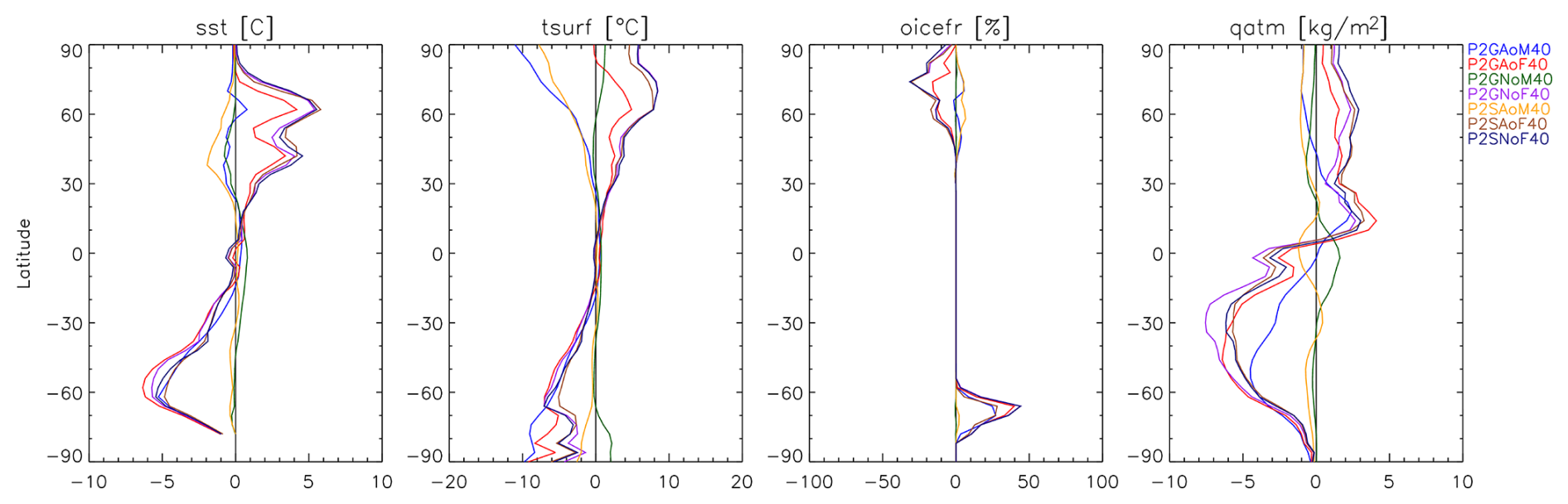
Figure 25Zonal mean difference from P2SNoM40 for sea surface temperature (sst; first panel), surface air temperature (tsurf; second panel), ocean and lake ice fraction (oicefr; third panel), and total atmospheric water vapor load (qatm; last panel).
5.6 Reproducibility of results
In the development and distribution of the source code of ROCKE-3D, we pay particular attention to model reproducibility, which is a widespread problem across many science domains (e.g., Donoho et al., 2008). For that reason, we only update the code by either adding diagnostics that do not change the model results or fixing key bugs and adding functionality using the opt-in approach discussed in Sect. 4.3 and Appendix B. Any major development happens in a separate branch of the code repository, which will eventually be distributed at a future date as a future ROCKE-3D model version (e.g., 2.1 or 3.0). However, exact reproducibility is frequently impossible for hardware purposes: different computer architectures, different compilers with different optimizations, and different ways to compile the model even on the same computer introduce numerical noise which, when propagated, does not allow one to exactly reproduce model simulations of any complexity, let alone a three-dimensional GCM like ROCKE-3D. This numerical noise though is random and does not introduce biases, which means that the climatologies calculated by any computer are virtually identical after long integrations. Long integrations are needed regardless for a proper analysis of results, so a change of computer is not expected to affect results qualitatively, and even quantitatively any change will not be statistically significant. This ensures that the model version presented here, including its updates described in Sect. 4.6.2, will generate qualitatively the same, but not identical, results on all computer architectures.
As described in more detail in the “Data availability” section below, we distribute all results presented here to the public, so that they can be used in any way deemed necessary. This includes, but is not limited to, further analyses not presented here; evaluation of simulations performed by others indicating that their climatologies are indeed the same; and continuation of simulations using small changes in physics or model parameters, in order to avoid long spinup times.
ROCKE-3D tutorials have been held annually since 2017. Participation has been in person and remote, with extensive online documentation that explains how to install supporting software requirements (ROCKE-3D compilers and libraries, 2022) and the model itself (ROCKE-3D installation, 2022). These are currently live documents hosted on Google Docs that are updated as operating system versions change and the supporting software is updated, often in step with operating system updates. The presentation slides are also hosted on Google Slides as they are updated year by year (ROCKE-3D tutorial slides, 2022). The tutorials are also recorded and placed on the GISS YouTube channel (ROCKE-3D tutorial video, 2022). This allows anyone in the world to access all materials at any time of year.
The ROCKE-3D simulations presented here have addressed limits to the encoded physics, parameterizations of key processes, and inconsistencies that become more apparent in scenarios beyond modern Earth, possibly impacting future projections and past simulations. This was achieved by (a) systematically studying how Earth-centric parameterizations, or the absence of them, affect model results and (b) exploring the role different parameterizations have on an Earth-like simulation by studying the role of the radiation scheme chosen (GISS vs. SOCRATES), the impact of changing atmospheric composition (presence/absence of oxygen and aerosols), the role of how ocean is parameterized (prescribed; Q-flux = 0; dynamic), and the role of horizontal resolution (4×5 vs. 2×2.5 in the atmosphere and 4×5 vs. 1×1.125 in the ocean in latitude and longitude). We also presented new components of the model, like the geothermal heat flux, an expansion of the dynamic lakes, the ability to simulate thin atmospheres, an improved and much more capable calendar system, and several other updates since ROCKE-3D version 1.0 (Way et al., 2017).
We discussed the importance of radiative balance and how to achieve it in a new world, and we explained how to identify how much spinup time is needed when starting from non-equilibrium conditions and how to create a new planet. We also described planetary configurations that are available to users, including several ancient Earth options, Venus, Mars, the transient atmosphere of the Early Moon, and other rocky exoplanets like those orbiting the Proxima Centauri b and Trappist systems, and how to use idealized land–ocean configurations, including aquaplanets. We made extensive analyses about influential parameters that users need to be aware of when using ROCKE-3D, including their role, valid ranges (where applicable), and important caveats when modified. These include ways to continue simulations in the case of a crash. Lastly, we presented some important information about the reproducibility of results.
Several future development tasks have already been identified, and we are actively pursuing them. We are working on enabling the prognostic calculation of a variable mean molecular weight of the atmosphere, which would allow the inclusion of water vapor and condensate in the mass and heat of the atmosphere. We are also including the option to simulate multiple condensable species, which would allow a mixed water–CO2 ice presence on Mars and CH4 ice on Titan. We are also working on merging the cloud microphysics calculations from the Earth parent model, which will be used for CMIP7, with ROCKE-3D, which will allow more realistic cloud calculations in other planets. Other minor developments continue to be implemented in the model, in what will eventually become ROCKE-3D v3.0 in the future.
The ROCKE-3D development continues to contribute to making a more robust ModelE for modern Earth climate science by questioning model assumptions and pushing capabilities through research on the Earth through time and exoplanet habitability. The model code and tutorials on how it can be installed and used by new users are publicly available.
Other than the science-relevant updates described in the paper, there are many other minor updates, which do affect model users that want to update their code to the newest version. These are listed below. It has to be noted that only the few changes that are ported to ROCKE-3D 2.0 from the updated ModelE 2.1 and affect the model's climate independently of prognostic tracers are listed here. The tracer code which affects the prognostic atmospheric composition has received much larger changes, but these are not the subject of this work. In most cases, although not all, the tracer updates were also less substantial.
A structural change that introduced only numerical noise differences from the original implementation is that the handling of greenhouse gases was taken out of the radiation code and is now present in its own module (GHGMOD). Another difference that was ported in is a unit change in the arrays that hold atmospheric mass (and tracer amounts, if enabled) from kg per grid box to kg m−2.
A new option in ROCKE-3D 2.0 (PCLD_INDICES_LOCAL) avoids a possible array indexing error in computing the fraction of high-level clouds (pcldh) if the model top pressure is greater than 680 mbar. It also avoids the possible non-physical artifacts of non-zero pcldl and pcldm being possible in model columns with surface pressure less than 680 and 480 mbar, respectively.
The selected options listed below need to be defined in the model rundecks prior to compilation. The model has many more additional ways to change its configuration and behavior which extend far beyond the scope of this paper.
Table B1Opt-in configuration changes that modify the default model behavior in a significant way.
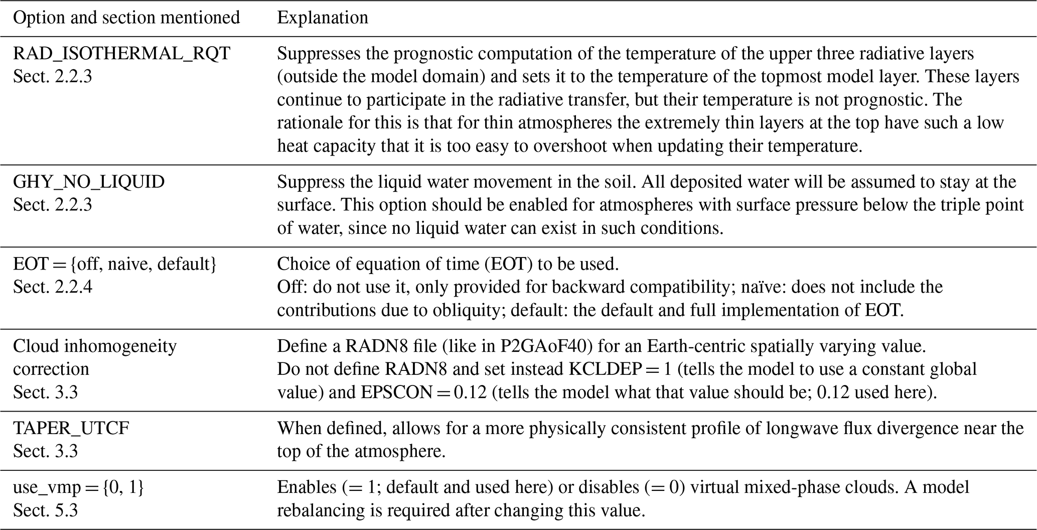
Table C1List of spectral files provided with ROCKE-3D for operation with SOCRATES. Unless otherwise indicated in the description, spectral files use HITRAN 2012 and have a maximum pressure and temperature of 1 bar and 400 K, respectively. All spectral files contain H2O and use the MT-CKD water vapor continuum model (Mlawer et al., 2012). For more details refer to the online documentation (ROCKE-3D spectral files).
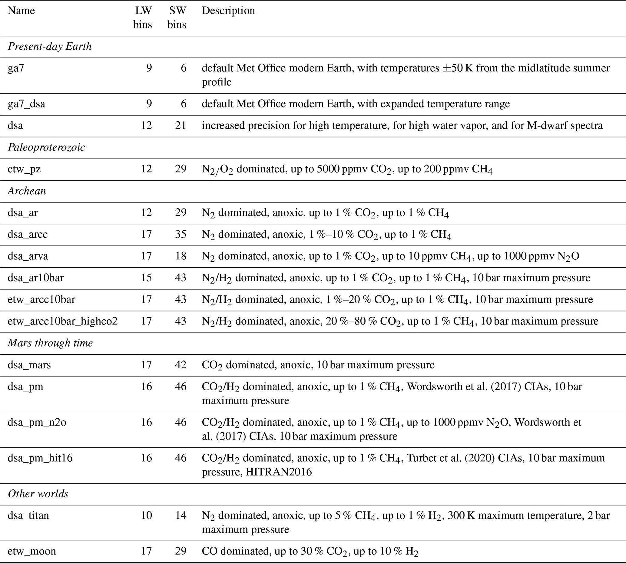
Table C2List of stellar spectra provided with ROCKE-3D for operation with SOCRATES. Stellar spectra are crafted either from exact replication or interpolation of theoretical spectra from the BT-Settl and BT-NextGen grid of models (e.g., Allard, 2013), with specifications and sources shown in the description column.
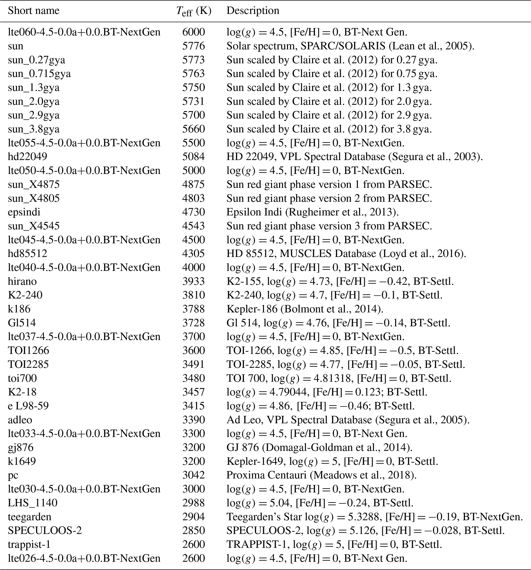
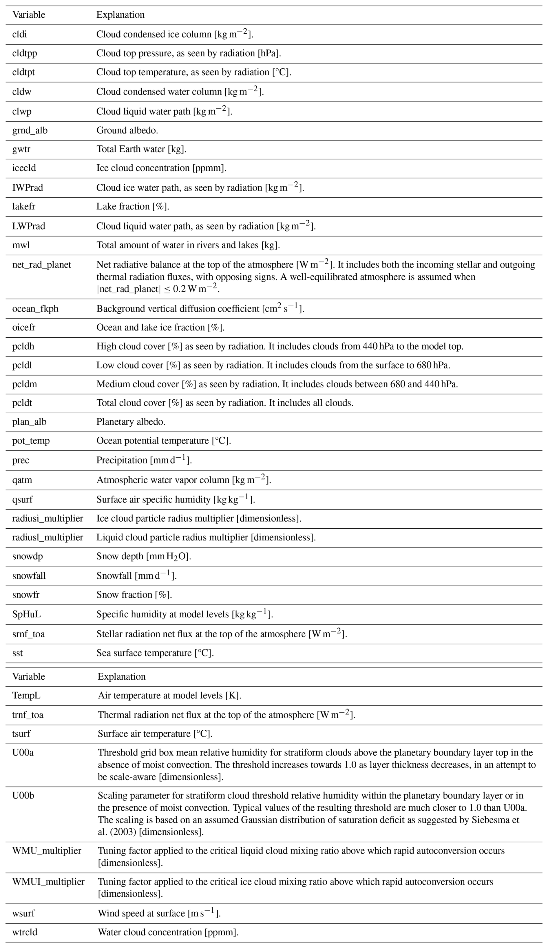
The ROCKE-3D model is publicly available at https://simplex.giss.nasa.gov/gcm/ROCKE-3D/ (NASA, 2025). The model code, all output, and the model configurations used here are available on a Zenodo archive (https://doi.org/10.5281/zenodo.14721184, Tsigaridis et al., 2025). All ROCKE-3D prescribed ocean configurations listed in Table 3, as well as their Q-flux = 0 and dynamic ocean equivalent configurations analyzed here, are provided as the template “rundecks” and the configuration files of the model, using the same naming convention and modified as described in Sect. 4.3 together with the model code.
All NetCDF data used in this and other publications of ROCKE-3D can be downloaded from the NCCS data portal: https://portal.nccs.nasa.gov/GISS_modelE/ROCKE-3D/publication-supplements/ (NCCS, 2025a). SOCRATES spectral files are also available from the same portal: https://portal.nccs.nasa.gov/GISS_modelE/ROCKE-3D/spectral_files/ (NCCS, 2025a).
A Zenodo archive (https://doi.org/10.5281/zenodo.14721184, Tsigaridis et al., 2025) with data from this work includes (1) all rundecks used in this work, for users to be able to reproduce our simulations; (2) all restart files at the end of the equilibration period for all simulations listed in Fig. 6 and throughout the paper, for simulation continuations without the need of a spinup; (3) time series of globally and annually averaged quantities in the atmosphere from the start of each simulation, including spinup, a small subset of which have been used to create Fig. 7; and (4) spatially varying climatological annual means of all atmospheric model output which was used for all maps presented in the paper. These data are also available in the NCCS data portal (https://portal.nccs.nasa.gov/GISS_modelE/ROCKE-3D/publication-supplements/Tsigaridis2025GMD-planet_2.0/) together with the individual years that constructed the climatologies, which are too voluminous for Zenodo to host.
KT and ADDG designed the work. KT, ADDG, and MK performed the model balancing. KT ran all simulations and made most of the plots. Others that made plots include CMC, LS, and MJW. ASA helped with the cloud diagnostics and analysis. IA developed the Moon configuration and the Mars configuration together with KT and JPP. MAC and LS worked on the alternate continental configurations. LS and RAR worked on the geothermal heat flux. TLC improved the calendar and added the equation of time. CMC and AL worked on the aquaplanet and ocean simulations. MJW worked on Venus and exoplanet simulations. NYK, GLR, RAR, and IA worked on the new surface hydrology physics. ETW worked on SOCRATES radiative transfer and radiation tables. KT wrote the first version of the manuscript and led subsequent edits with the help of all co-authors.
The contact author has declared that none of the authors has any competing interests.
Publisher's note: Copernicus Publications remains neutral with regard to jurisdictional claims made in the text, published maps, institutional affiliations, or any other geographical representation in this paper. While Copernicus Publications makes every effort to include appropriate place names, the final responsibility lies with the authors.
This work was supported by NASA's Nexus for Exoplanet System Science (NExSS) and the NASA Interdisciplinary Consortia for Astrobiology Research (ICAR). Further support for this research was provided by the NASA Earth and Planetary Science Division Research Programs, through ISFM work package ROCKE-3D at the Goddard Institute for Space Studies. We acknowledge support from the GSFC Sellers Exoplanet Environments Collaboration (SEEC), which is funded by the NASA Planetary Science Division's Internal Scientist Funding Model. Earth climate modeling at GISS is supported by the NASA Modeling, Analysis and Prediction program (MAP). Thin-atmosphere research was supported by NASA Solar System Workings program award 80NSSC21K0163. Resources supporting this work were provided by the NASA High-End Computing (HEC) Program through the NASA Center for Climate Simulation (NCCS) at Goddard Space Flight Center.
This research has been supported by the National Aeronautics and Space Administration, Goddard Space Flight Center, Nexus for Exoplanet System Science (NExSS), Interdisciplinary Consortia for Astrobiology Research (ICAR), ISFM work package ROCKE-3D at the Goddard Institute for Space Studies, Sellers Exoplanet Environments Collaboration (SEEC), Modeling, Analysis and Prediction program (MAP), and award 80NSSC21K0163.
This paper was edited by Paul Ullrich and reviewed by two anonymous referees.
Adcroft, A., Scott, J. R., and Marotzke, J.: Impact of geothermal heating on the global ocean circulation, Geophys. Res. Lett., 28, 1735–1738, https://doi.org/10.1029/2000GL012182, 2001.
Aleinov, I., Way, M. J., Harman, C., Tsigaridis, K., Wolf, E. T., and Gronoff, G.: Modeling a Transient Secondary Paleolunar Atmosphere: 3-D Simulations and Analysis, Geophys. Res. Lett., 46, 5107–5116, https://doi.org/10.1029/2019GL082494, 2019.
Allard, F.: The BT-Settl Model Atmospheres for Stars, Brown Dwarfs and Planets, Proc. Int. Astron. Union, 8, 271–272, https://doi.org/10.1017/S1743921313008545, 2013.
Amundsen, D. S., Mayne, N. J., Baraffe, I., Manners, J., Tremblin, P., Drummond, B., Smith, C., Acreman, D. M., and Homeier, D.: The UK Met Office global circulation model with a sophisticated radiation scheme applied to the hot Jupiter HD 209458b, Astron. Astrophys., 595, A36, https://doi.org/10.1051/0004-6361/201629183, 2016.
Amundsen, D. S., Tremblin, P., Manners, J., Baraffe, I., and Mayne, N. J.: Treatment of overlapping gaseous absorption with the correlated-k method in hot Jupiter and brown dwarf atmosphere models, Astron. Astrophys., 598, A97, https://doi.org/10.1051/0004-6361/201629322, 2017.
Aylmer, J., Ferreira, D., and Feltham, D.: Impacts of Oceanic and Atmospheric Heat Transports on Sea Ice Extent, J. Climate, 33, 7197–7215, https://doi.org/10.1175/JCLI-D-19-0761.1, 2020.
Batra, K. and Olson, S. L.: Climatic Effects of Ocean Salinity on M Dwarf Exoplanets, Astrophys. J. Lett., 971, L11, https://doi.org/10.3847/2041-8213/ad63a5, 2024.
Bauer, S. E., Tsigaridis, K., Faluvegi, G., Kelley, M., Lo, K. K., Miller, R. L., Nazarenko, L., Schmidt, G. A., and Wu, J.: Historical (1850–2014) aerosol evolution and role on climate forcing using the GISS ModelE2.1 contribution to CMIP6, J. Adv. Model. Earth Syst., 12, e2019MS001978, https://doi.org/10.1029/2019MS001978, 2020.
Berger, A., M.-F. Loutre, and C. Tricot: Insolation and Earth's orbital periods, J. Geophys. Res., 98, 10341–10362, https://doi.org/10.1029/93JD00222, 1993.
Bìhounková, M., Tobie, G., Choblet, G., and Èadek, O.: Coupling mantle convection and tidal dissipation: Applications to Enceladus and Earth-like planets, J. Geophys. Res.-Planets, 115, E09011, https://doi.org/10.1029/2009JE003564, 2010.
Bitz, C. M., Holland, M. M., Hunke, E. C., and Moritz, R. E.: Maintenance of the Sea-Ice Edge, J. Climate, 18, 2903–2921, https://doi.org/10.1175/JCLI3428.1, 2005.
Bolmont, E., Raymond, S. N., von Paris, P., Selsis, F., Hersant, F., Quintana, E. V., and Barclay, T.: Formation, tidal evolution, and habitability of the KEPLER-186 System, Astrophys. J., 793, 3, https://doi.org/10.1088/0004-637X/793/1/3, 2014.
Bougher, S. W., Hunten, D. M., Phillips, R. J., Matthews, M. S., Ruskin, A. S., and Guerrieri, M. L. (Eds.): Venus II: Geology, Geophysics, Atmosphere, and Solar Wind Environment, University of Arizona Press, https://doi.org/10.2307/j.ctv27tct5m, 1997.
Bouley, S., Baratoux, D., Matsuyama, I., Forget, F., Séjourné, A., Turbet, M., and Costard, F.: Late Tharsis formation and implications for early Mars, Nature, 531, 344–347, https://doi.org/10.1038/nature17171, 2016.
Brunetti, M., Kasparian, J., and Vérard, C.: Co-existing climate attractors in a coupled aquaplanet, Clim. Dynam., 53, 6293–6308, https://doi.org/10.1007/s00382-019-04926-7, 2019.
Bryan, K.: A numerical method for the study of the circulation of the world ocean, J. Comput. Phys., 4, 347–376, https://doi.org/10.1016/0021-9991(69)90004-7, 1969.
Bryan, K.: Poleward Heat Transport by the Ocean: Observations and Models, Annu. Rev. Earth Planet. Sci., 10, 15–38, https://doi.org/10.1146/annurev.ea.10.050182.000311, 1982.
Butcher, F. E. G., Balme, M. R., Gallagher, C., Arnold, N. S., Conway, S. J., Hagermann, A., and Lewis, S. R.: Recent Basal Melting of a Mid-Latitude Glacier on Mars, J. Geophys. Res.-Planets, 122, 2445–2468, https://doi.org/10.1002/2017JE005434, 2017.
Claire, M. W., Sheets, J., Cohen, M., Ribas, I., Meadows, V. S., and Catling, D. C.: the evolution of solar flux from 0.1 nm to 160 µm: quantitative estimates for planetary studies, Astrophys. J., 757, 95, https://doi.org/10.1088/0004-637X/757/1/95, 2012.
Colose, C. M., Haqq-Misra, J., Wolf, E. T., Del Genio, A. D., Barnes, R., Way, M. J., and Ruedy, R.: Effects of Spin–Orbit Resonances and Tidal Heating on the Inner Edge of the Habitable Zone, Astrophys. J., 921, 25, https://doi.org/10.3847/1538-4357/ac135c, 2021.
Davies, J. H.: Global map of solid Earth surface heat flow, Geochem. Geophy., Geosy., 14, 4608–4622, https://doi.org/10.1002/ggge.20271, 2013.
Del Genio, A. D., Yao, M.-S., Kovari, W., and Lo, K. K.-W.: A Prognostic Cloud Water Parameterization for Global Climate Models, J. Climate, 9, 270–304, https://doi.org/10.1175/1520-0442(1996)009<0270:APCWPF>2.0.CO;2, 1996.
Del Genio, A. D., Way, M. J., Kiang, N. Y., Aleinov, I., Puma, M. J., and Cook, B.: Climates of Warm Earth-like Planets. III. Fractional Habitability from a Water Cycle Perspective, Astrophys. J., 887, 197, https://doi.org/10.3847/1538-4357/ab57fd, 2019a.
Del Genio, A. D., Way, M. J., Amundsen, D. S., Aleinov, I., Kelley, M., Kiang, N. Y., and Clune, T. L.: Habitable Climate Scenarios for Proxima Centauri b with a Dynamic Ocean, Astrobiology, 19, 99–125, https://doi.org/10.1089/ast.2017.1760, 2019b.
Domagal-Goldman, S. D., Segura, A., Claire, M. W., Robinson, T. D., and Meadows, V. S.: Abiotic ozone and oxygen in atmospheres similar to prebiotic Earth, Astrophys. J., 792, 90, https://doi.org/10.1088/0004-637X/792/2/90, 2014.
Donoho, D. L., Maleki, A., Rahman, I. U., Shahram, M., and Stodden, V.: Reproducible Research in Computational Harmonic Analysis, Computing in Science & Engineering, 11, 8–18, https://doi.org/10.1109/MCSE.2009.15, 2009.
Edwards, J. M.: Efficient Calculation of Infrared Fluxes and Cooling Rates Using the Two-Stream Equations, J. Atmos. Sci., 53, 1921–1932, https://doi.org/10.1175/1520-0469(1996)053<1921:ECOIFA>2.0.CO;2, 1996.
Edwards, J. M. and Slingo, A.: Studies with a flexible new radiation code. I: Choosing a configuration for a large-scale model, Q. J. Roy. Meteorol. Soc., 122, 689–719, https://doi.org/10.1002/qj.49712253107, 1996.
Emile-Geay, J. and Madec, G.: Geothermal heating, diapycnal mixing and the abyssal circulation, Ocean Sci., 5, 203–217, https://doi.org/10.5194/os-5-203-2009, 2009.
Eyring, V., Bony, S., Meehl, G. A., Senior, C. A., Stevens, B., Stouffer, R. J., and Taylor, K. E.: Overview of the Coupled Model Intercomparison Project Phase 6 (CMIP6) experimental design and organization, Geosci. Model Dev., 9, 1937–1958, https://doi.org/10.5194/gmd-9-1937-2016, 2016.
Fauchez, T. J., Turbet, M., Wolf, E. T., Boutle, I., Way, M. J., Del Genio, A. D., Mayne, N. J., Tsigaridis, K., Kopparapu, R. K., Yang, J., Forget, F., Mandell, A., and Domagal Goldman, S. D.: TRAPPIST-1 Habitable Atmosphere Intercomparison (THAI): motivations and protocol version 1.0, Geosci. Model Dev., 13, 707–716, https://doi.org/10.5194/gmd-13-707-2020, 2020.
Fauchez, T. J., Villanueva, G. L., Sergeev, D. E., Turbet, M., Boutle, I. A., Tsigaridis, K., Way, M. J., Wolf, E. T., Domagal-Goldman, S. D., Forget, F., Haqq-Misra, J., Kopparapu, R. K., Manners, J., and Mayne, N. J.: The TRAPPIST-1 Habitable Atmosphere Intercomparison (THAI). III. Simulated Observables – the Return of the Spectrum, Planet. Sci. J., 3, 213, https://doi.org/10.3847/PSJ/ac6cf1, 2022.
Ferreira, D., Marshall, J., and Rose, B.: Climate Determinism Revisited: Multiple Equilibria in a Complex Climate Model, J. Climate, 24, 992–1012, https://doi.org/10.1175/2010JCLI3580.1, 2011.
Forget, F., Bertrand, T., Vangvichith, M., Leconte, J., Millour, E., and Lellouch, E.: A post-new horizons global climate model of Pluto including the N2, CH4 and CO cycles, Icarus, 287, 54–71, https://doi.org/10.1016/j.icarus.2016.11.038, 2017.
Guzewich, S. D., Way, M. J., Aleinov, I., Wolf, E. T., Del Genio, A., Wordsworth, R., and Tsigaridis, K.: 3D Simulations of the Early Martian Hydrological Cycle Mediated by a H2-CO2 Greenhouse, J. Geophys. Res.-Planets, 126, e2021JE006825, https://doi.org/10.1029/2021JE006825, 2021.
Hansen, J., Russell, G., Rind, D., Stone, P., Lacis, A., Lebedeff, S., Ruedy, R., and Travis, L.: Efficient Three-Dimensional Global Models for Climate Studies: Models I and II, Mon. Weather Rev., 111, 609–662, 1983.
Haywood, A. M., Dowsett, H. J., Dolan, A. M., Rowley, D., Abe-Ouchi, A., Otto-Bliesner, B., Chandler, M. A., Hunter, S. J., Lunt, D. J., Pound, M., and Salzmann, U.: The Pliocene Model Intercomparison Project (PlioMIP) Phase 2: scientific objectives and experimental design, Clim. Past, 12, 663–675, https://doi.org/10.5194/cp-12-663-2016, 2016.
Held, I. M.: The Partitioning of the Poleward Energy Transport between the Tropical Ocean and Atmosphere, J. Atmos. Sci., 58, 943–948, https://doi.org/10.1175/1520-0469(2001)058<0943:TPOTPE>2.0.CO;2, 2001.
Hendrix, A. R., Hurford, T. A., Barge, L. M., Bland, M. T., Bowman, J. S., Brinckerhoff, W., Buratti, B. J., Cable, M. L., Castillo-Rogez, J., Collins, G. C., Diniega, S., German, C. R., Hayes, A. G., Hoehler, T., Hosseini, S., Howett, C. J. A., McEwen, A. S., Neish, C. D., Neveu, M., Nordheim, T. A., Patterson, G. W., Patthoff, D. A., Phillips, C., Rhoden, A., Schmidt, B. E., Singer, K. N., Soderblom, J. M., and Vance, S. D.: The NASA Roadmap to Ocean Worlds, Astrobiology, 19, 1–27, https://doi.org/10.1089/ast.2018.1955, 2019.
Henning, W. G. and Hurford, T.: Tidal heating in multilayered terrestrial exoplanets, Astrophys. J., 789, 30, https://doi.org/10.1088/0004-637X/789/1/30, 2014.
Hofmann, M. and Maqueda, M. A.: Geothermal heat flux and its influence on the oceanic abyssal circulation and radiocarbon distribution, Geophys. Res. Lett., 36, L03603, https://doi.org/10.1029/2008GL036078, 2009.
Hörner, J. and Voigt, A.: Sea-ice thermodynamics can determine waterbelt scenarios for Snowball Earth, Earth Syst. Dynam., 15, 215–223, https://doi.org/10.5194/esd-15-215-2024, 2024.
Hu, Y. and Yang, J.: Role of ocean heat transport in climates of tidally locked exoplanets around M dwarf stars, P. Natl. Acad. Sci. USA, 111, 629–634, https://doi.org/10.1073/pnas.1315215111, 2014.
IPCC – Intergovernmental Panel on Climate Change (Ed.): The Earth's Energy Budget, Climate Feedbacks and Climate Sensitivity, in: Climate Change 2021 – The Physical Science Basis: Working Group I Contribution to the Sixth Assessment Report of the Intergovernmental Panel on Climate Change, Cambridge University Press, Cambridge, 923–1054, https://doi.org/10.1017/9781009157896.009, 2023.
Ito, G., Romanou, A., Kiang, N. Y., Faluvegi, G., Aleinov, I., Ruedy, R., Russell, G., Lerner, P., Kelley, M., and Lo, K.: Global Carbon Cycle and Climate Feedbacks in the NASA GISS ModelE2.1, J. Adv. Model. Earth Syst., 12, e2019MS002030, https://doi.org/10.1029/2019MS002030, 2020.
Johns, T. C., Carnell, R. E., Crossley, J. F., Gregory, J. M., Mitchell, J. F. B., Senior, C. A., Tett, S. F. B., and Wood, R. A.: The second Hadley Centre coupled ocean-atmosphere GCM: model description, spinup and validation, Clim. Dynam., 13, 103–134, https://doi.org/10.1007/s003820050155, 1997.
Jones, C. D., Arora, V., Friedlingstein, P., Bopp, L., Brovkin, V., Dunne, J., Graven, H., Hoffman, F., Ilyina, T., John, J. G., Jung, M., Kawamiya, M., Koven, C., Pongratz, J., Raddatz, T., Randerson, J. T., and Zaehle, S.: C4MIP – The Coupled Climate–Carbon Cycle Model Intercomparison Project: experimental protocol for CMIP6, Geosci. Model Dev., 9, 2853–2880, https://doi.org/10.5194/gmd-9-2853-2016, 2016.
Kelley, M., Schmidt, G. A., Nazarenko, L. S., Bauer, S. E., Ruedy, R., Russell, G. L., Ackerman, A. S., Aleinov, I., Bauer, M., Bleck, R., Canuto, V., Cesana, G., Cheng, Y., Clune, T. L., Cook, B. I., Cruz, C. A., Del Genio, A. D., Elsaesser, G. S., Faluvegi, G., Kiang, N. Y., Kim, D., Lacis, A. A., Leboissetier, A., LeGrande, A. N., Lo, K. K., Marshall, J., Matthews, E. E., McDermid, S., Mezuman, K., Miller, R. L., Murray, L. T., Oinas, V., Orbe, C., García-Pando, C. P., Perlwitz, J. P., Puma, M. J., Rind, D., Romanou, A., Shindell, D. T., Sun, S., Tausnev, N., Tsigaridis, K., Tselioudis, G., Weng, E., Wu, J., and Yao, M.-S.: GISS-E2.1: Configurations and Climatology, J. Adv. Model. Earth Syst., 12, e2019MS002025, https://doi.org/10.1029/2019MS002025, 2020.
Kim, Y., Moorcroft, P. R., Aleinov, I., Puma, M. J., and Kiang, N. Y.: Variability of phenology and fluxes of water and carbon with observed and simulated soil moisture in the Ent Terrestrial Biosphere Model (Ent TBM version 1.0.1.0.0), Geosci. Model Dev., 8, 3837–3865, https://doi.org/10.5194/gmd-8-3837-2015, 2015.
Klinger, B. A. and Marotzke, J.: Meridional Heat Transport by the Subtropical Cell, J. Phys. Oceanogr., 30, 696–705, https://doi.org/10.1175/1520-0485(2000)030<0696:MHTBTS>2.0.CO;2, 2000.
Kopparapu, R. K., Ramirez, R., Kasting, J. F., Eymet, V., Robinson, T. D., Mahadevan, S., Terrien, R. C., Domagal-Goldman, S., Meadows, V., and Deshpande, R.: Habitable zones around main-sequence stars: new estimates, Astrophys. J., 765, 131, https://doi.org/10.1088/0004-637X/765/2/131, 2013.
Lacis, A. A. and Oinas, V.: A Description of the Correlated k Distribution Method for Modeling Nongray Gaseous Absorption, Thermal Emission, and Multiple Scattering in Vertically Inhomogeneous Atmospheres, J. Geophys. Res.-Atmos., 96, 9027–9063, https://doi.org/10.1029/90jd01945, 1991.
Lean, J., Rottman, G., Harder, J., and Kopp, G.: SORCE Contributions to New Understanding of Global Change and Solar Variability, Solar Phys., 230, 27–53, https://doi.org/10.1007/s11207-005-1527-2, 2005.
Levitus, S. and Boyer, T. P.: World ocean atlas 1994, in: Vol. 4, Temperature, https://repository.library.noaa.gov/view/noaa/1381 (last access: 2 September 2025), 1994.
Levitus, S., Burgett, R., and Boyer, T. P.: World ocean atlas 1994, in: Vol. 3, Salinity, https://repository.library.noaa.gov/view/noaa/1382 (last access: 2 September 2025), 1994.
Loyd, R. O. P., France, K., Youngblood, A., Schneider, C., Brown, A., Hu, R., Linsky, J., Froning, C. S., Redfield, S., Rugheimer, S., and Tian, F.: the muscles treasury survey. III. X-ray to infrared spectra of 11 M and K stars hosting planets, Astrophys. J., 824, 102, https://doi.org/10.3847/0004-637X/824/2/102, 2016.
Manabe, S. and Stouffer, R. J.: Century-scale effects of increased atmospheric C02 on the ocean–atmosphere system, Nature, 364, 215–218, https://doi.org/10.1038/364215a0, 1993.
Manabe, S. and Wetherald, R. T.: Thermal Equilibrium of the Atmosphere with a Given Distribution of Relative Humidity, J. Atmos. Sci., 24, 241–259, https://doi.org/10.1175/1520-0469(1967)024<0241:TEOTAW>2.0.CO;2, 1967.
Marshall, J., Hill, C., Perelman, L., and Adcroft, A.: Hydrostatic, quasi-hydrostatic, and nonhydrostatic ocean modeling, J. Geophys. Res.-Oceans, 102, 5733–5752, https://doi.org/10.1029/96JC02776, 1997.
Meadows, V. S., Arney, G. N., Schwieterman, E. W., Lustig-Yaeger, J., Lincowski, A. P., Robinson, T., Domagal-Goldman, S. D., Deitrick, R., Barnes, R. K., Fleming, D. P., Luger, R., Driscoll, P. E., Quinn, T. R., and Crisp, D.: The Habitability of Proxima Centauri b: Environmental States and Observational Discriminants, Astrobiology, 18, 133–189, https://doi.org/10.1089/ast.2016.1589, 2018.
Miller, J. R., Russell, G. L., and Tsang, L.-C.: Annual oceanic heat transports computed from an atmospheric model, Dynam. Atmos. Oceans, 7, 95–109, https://doi.org/10.1016/0377-0265(83)90012-X, 1983.
Miller, R. L., Schmidt, G. A., Nazarenko, L. S., Bauer, S. E., Kelley, M., Ruedy, R., Russell, G. L., Ackerman, A. S., Aleinov, I., Bauer, M., Bleck, R., Canuto, V., Cesana, G., Cheng, Y., Clune, T. L., Cook, B. I., Cruz, C. A., Del Genio, A. D., Elsaesser, G. S., Faluvegi, G., Kiang, N. Y., Kim, D., Lacis, A. A., Leboissetier, A., LeGrande, A. N., Lo, K. K., Marshall, J., Matthews, E. E., McDermid, S., Mezuman, K., Murray, L. T., Oinas, V., Orbe, C., Pérez García-Pando, C., Perlwitz, J. P., Puma, M. J., Rind, D., Romanou, A., Shindell, D. T., Sun, S., Tausnev, N., Tsigaridis, K., Tselioudis, G., Weng, E., Wu, J., and Yao, M.-S.: CMIP6 Historical Simulations (1850–2014) With GISS-E2.1, J. Adv. Model. Earth Syst., 13, e2019MS002034, https://doi.org/10.1029/2019MS002034, 2021.
Mlawer, E. J., Payne, V. H., Moncet, J.-L., Delamere, J. S., Alvarado, M. J., and Tobin, D. C.: Development and recent evaluation of the MT_CKD model of continuum absorption, Philos. T. Roy. Soc. A, 370, 2520–2556, https://doi.org/10.1098/rsta.2011.0295, 2012.
Munk, W. and Wunsch, C.: Abyssal recipes II: energetics of tidal and wind mixing, Deep-Sea Res. Pt. I, 45, 1977–2010, https://doi.org/10.1016/S0967-0637(98)00070-3, 1998.
NASA: ROCKE-3D, NASA [code], https://simplex.giss.nasa.gov/gcm/ROCKE-3D/ (last access: 2 September 2025), 2025.
Nazarenko, L. S., Tausnev, N., Russell, G. L., Rind, D., Miller, R. L., Schmidt, G. A., Bauer, S. E., Kelley, M., Ruedy, R., Ackerman, A. S., Aleinov, I., Bauer, M., Bleck, R., Canuto, V., Cesana, G., Cheng, Y., Clune, T. L., Cook, B. I., Cruz, C. A., Del Genio, A. D., Elsaesser, G. S., Faluvegi, G., Kiang, N. Y., Kim, D., Lacis, A. A., Leboissetier, A., LeGrande, A. N., Lo, K. K., Marshall, J., Matthews, E. E., McDermid, S., Mezuman, K., Murray, L. T., Oinas, V., Orbe, C., García-Pando, C. P., Perlwitz, J. P., Puma, M. J., Romanou, A., Shindell, D. T., Sun, S., Tsigaridis, K., Tselioudis, G., Weng, E., Wu, J., and Yao, M.-S.: Future Climate Change Under SSP Emission Scenarios With GISS-E2.1, J. Adv. Model. Earth Syst., 14, e2021MS002871, https://doi.org/10.1029/2021MS002871, 2022.
NCCS: ROCKE-3D output, Goddard [data set], https://portal.nccs.nasa.gov/GISS_modelE/ROCKE-3D/publication-supplements/ (last access: 2 September 2025), 2025a.
NCCS: SOCRATES spectral files, Goddard [data set], https://portal.nccs.nasa.gov/GISS_modelE/ROCKE-3D/spectral_files/ (last access: 2 September 2025), 2025b.
Needham, D. H. and Kring, D. A.: Lunar volcanism produced a transient atmosphere around the ancient Moon, Earth Planet. Sc. Lett., 478, 175–178, https://doi.org/10.1016/j.epsl.2017.09.002, 2017.
Phillips, N. A.: The general circulation of the atmosphere: A numerical experiment, Q. J. Roy. Meteorol. Soc., 82, 123–164, https://doi.org/10.1002/qj.49708235202, 1956.
Pierrehumbert, R. T.: A palette of climates for Gliese 581g, Astrophys. J. Lett., 726, L8, https://doi.org/10.1088/2041-8205/726/1/L8, 2010.
Prather, M. J.: Numerical advection by conservation of second-order moments, J. Geophys. Res.-Atmos., 91, 6671–6681, https://doi.org/10.1029/JD091iD06p06671, 1986.
Rencurrel, M. C. and Rose, B. E. J.: Exploring the Climatic Response to Wide Variations in Ocean Heat Transport on an Aquaplanet, J. Climate, 31, 6299–6318, https://doi.org/10.1175/JCLI-D-17-0856.1, 2018.
Rind, D. and Lerner, J.: Use of on-line tracers as a diagnostic tool in general circulation model development: 1. Horizontal and vertical transport in the troposphere, J. Geophys. Res.=Atmos., 101, 12667–12683, https://doi.org/10.1029/96JD00551, 1996.
Rind, D., Orbe, C., Jonas, J., Nazarenko, L., Zhou, T., Kelley, M., Lacis, A., Shindell, D., Faluvegi, G., Romanou, A., Russell, G., Tausnev, N., Bauer, M., and Schmidt, G.: GISS Model E2.2: A Climate Model Optimized for the Middle Atmosphere – Model Structure, Climatology, Variability, and Climate Sensitivity, J. Geophys. Res.-Atmos., 125, e2019JD032204, https://doi.org/10.1029/2019JD032204, 2020.
ROCKE-3D compilers and libraries: https://tinyurl.com/ROCKE3D-compilerslibraries (last access: 25 July 2022), 2022.
ROCKE-3D installation: https://tinyurl.com/ROCKE3D-install (last access: 25 July 2022), 2022.
ROCKE-3D spectral files: https://tinyurl.com/ROCKE3D-spectralfiles (last access: 25 July 2022), 2022.
ROCKE-3D tutorial slides: https://tinyurl.com/ROCKE3D-tutorialslides (last access: 25 July 2022), 2022.
ROCKE-3D tutorial video: https://tinyurl.com/ROCKE3D-tutorialvideo (last access: 25 July 2022), 2022.
Romanou, A., Rind, D., Jonas, J., Miller, R., Kelley, M., Russell, G., Orbe, C., Nazarenko, L., Latto, R., and Schmidt, G. A.: Stochastic Bifurcation of the North Atlantic Circulation under a Midrange Future Climate Scenario with the NASA-GISS ModelE, J. Climate, 36, 6141–6161, https://doi.org/10.1175/JCLI-D-22-0536.1, 2023.
Rose, B. E. J.: Stable “Waterbelt” climates controlled by tropical ocean heat transport: A nonlinear coupled climate mechanism of relevance to Snowball Earth, J. Geophys. Res.-Atmos., 120, 1404–1423, https://doi.org/10.1002/2014JD022659, 2015.
Rose, B. E. J., Ferreira, D., and Marshall, J.: The Role of Oceans and Sea Ice in Abrupt Transitions between Multiple Climate States, J. Climate, 26, 2862–2879, https://doi.org/10.1175/JCLI-D-12-00175.1, 2013.
Rosenzweig, C. and Abramopoulos, F.: Land-Surface Model Development for the GISS GCM, J. Climate, 10, 2040–2054, https://doi.org/10.1175/1520-0442(1997)010<2040:LSMDFT>2.0.CO;2, 1997.
Rossow, W. B., Delo, C., and Cairns, B.: Implications of the Observed Mesoscale Variations of Clouds for the Earth's Radiation Budget, J. Climate, 15, 557–585, https://doi.org/10.1175/1520-0442(2002)015<0557:IOTOMV>2.0.CO;2, 2002.
Rugheimer, S., Kaltenegger, L., Zsom, A., Segura, A., and Sasselov, D.: Spectral Fingerprints of Earth-like Planets Around FGK Stars, Astrobiology, 13, 251–269, https://doi.org/10.1089/ast.2012.0888, 2013.
Russell, G. L., Miller, J. R., and Tsang, L.-C.: Seasonal oceanic heat transports computed from an atmospheric model, Dynam. Atmos. Oceans, 9, 253–271, https://doi.org/10.1016/0377-0265(85)90022-3, 1985.
Russell, G. L., Miller, J. R., and Rind, D.: A coupled atmosphere-ocean model for transient climate change studies, Atmosphere-Ocean, 33, 683–730, 1995.
Schmidt, F., Way, M. J., Costard, F., Bouley, S., Séjourné, A., and Aleinov, I.: Circumpolar ocean stability on Mars 3 Gy ago, P. Natl. Acad. Sci. USA, 119, e2112930118, https://doi.org/10.1073/pnas.2112930118, 2022.
Schmidt, G. A., Bitz, C. M., Mikolajewicz, U., and Tremblay, L.-B.: Ice–ocean boundary conditions for coupled models, Ocean Model., 7, 59–74, https://doi.org/10.1016/S1463-5003(03)00030-1, 2004.
Schmidt, G. A., Ruedy, R., Hansen, J. E., Aleinov, I., Bell, N., Bauer, M., Bauer, S., Cairns, B., Canuto, V., Cheng, Y., Del Genio, A., Faluvegi, G., Friend, A. D., Hall, T. M., Hu, Y. Y., Kelley, M., Kiang, N. Y., Koch, D., Lacis, A. A., Lerner, J., Lo, K. K., Miller, R. L., Nazarenko, L., Oinas, V., Perlwitz, J., Rind, D., Romanou, A., Russell, G. L., Sato, M., Shindell, D. T., Stone, P. H., Sun, S., Tausnev, N., Thresher, D., and Yao, M. S.: Present-day atmospheric simulations using GISS ModelE: Comparison to in situ, satellite, and reanalysis data, J. Climate, 19, 153–192, https://doi.org/10.1175/jcli3612.1, 2006.
Schmidt, G. A., Kelley, M., Nazarenko, L., Ruedy, R., Russell, G. L., Aleinov, I., Bauer, M., Bauer, S. E., Bhat, M. K., Bleck, R., Canuto, V., Chen, Y.-H., Cheng, Y., Clune, T. L., Del Genio, A., de Fainchtein, R., Faluvegi, G., Hansen, J. E., Healy, R. J., Kiang, N. Y., Koch, D., Lacis, A. A., LeGrande, A. N., Lerner, J., Lo, K. K., Matthews, E. E., Menon, S., Miller, R. L., Oinas, V., Oloso, A. O., Perlwitz, J. P., Puma, M. J., Putman, W. M., Rind, D., Romanou, A., Sato, M., Shindell, D. T., Sun, S., Syed, R. A., Tausnev, N., Tsigaridis, K., Unger, N., Voulgarakis, A., Yao, M.-S., and Zhang, J.: Configuration and assessment of the GISS ModelE2 contributions to the CMIP5 archive, J. Adv. Model. Earth Syst., 6, 141–184, https://doi.org/10.1002/2013MS000265, 2014.
Scott, J. R., Marotzke, J., and Adcroft, A.: Geothermal heating and its influence on the meridional overturning circulation, J. Geophys. Res.-Oceans, 106, 31141–31154, https://doi.org/10.1029/2000JC000532, 2001.
Seager, R., Battisti, D.S., Yin, J., Gordon, N., Naik, N., Clement, A.C. and Cane, M.A.: Is the Gulf Stream responsible for Europe's mild winters?, Q. J. R. Meteorol. Soc., 128, 2563–2586, https://doi.org/10.1256/qj.01.128, 2002.
Séférian, R., Berthet, S., Yool, A., Palmiéri, J., Bopp, L., Tagliabue, A., Kwiatkowski, L., Aumont, O., Christian, J., Dunne, J., Gehlen, M., Ilyina, T., John, J. G., Li, H., Long, M. C., Luo, J. Y., Nakano, H., Romanou, A., Schwinger, J., Stock, C., Santana-Falcón, Y., Takano, Y., Tjiputra, J., Tsujino, H., Watanabe, M., Wu, T., Wu, F., and Yamamoto, A.: Tracking Improvement in Simulated Marine Biogeochemistry Between CMIP5 and CMIP6, Curr. Clim. Change Rep., 6, 95–119, https://doi.org/10.1007/s40641-020-00160-0, 2020.
Segura, A., Krelove, K., Kasting, J. F., Sommerlatt, D., Meadows, V., Crisp, D., Cohen, M., and Mlawer, E.: Ozone Concentrations and Ultraviolet Fluxes on Earth-Like Planets Around Other Stars, Astrobiology, 3, 689–708, https://doi.org/10.1089/153110703322736024, 2003.
Segura, A., Kasting, J. F., Meadows, V., Cohen, M., Scalo, J., Crisp, D., Butler, R. A. H., and Tinetti, G.: Biosignatures from Earth-Like Planets Around M Dwarfs, Astrobiology, 5, 706–725, https://doi.org/10.1089/ast.2005.5.706, 2005.
Sergeev, D. E., Fauchez, T. J., Turbet, M., Boutle, I. A., Tsigaridis, K., Way, M. J., Wolf, E. T., Domagal-Goldman, S. D., Forget, F., Haqq-Misra, J., Kopparapu, R. K., Lambert, F. H., Manners, J., and Mayne, N. J.: The TRAPPIST-1 Habitable Atmosphere Intercomparison (THAI). II. Moist Cases – The Two Waterworlds, Planet. Sci. J., 3, 212, https://doi.org/10.3847/PSJ/ac6cf2, 2022.
Sergeev, D. E., Boutle, I. A., Lambert, F. H., Mayne, N. J., Bendall, T., Kohary, K., Olivier, E., and Shipway, B.: The Impact of the Explicit Representation of Convection on the Climate of a Tidally Locked Planet in Global Stretched-mesh Simulations, Astrophys. J., 970, 7, https://doi.org/10.3847/1538-4357/ad4ecd, 2024.
Shapiro, R.: Smoothing, filtering, and boundary effects, Rev. Geophys., 8, 359–387, https://doi.org/10.1029/RG008i002p00359, 1970.
Shapiro, R.: Linear filtering, Math. Comp., 29, 1094–1097, https://doi.org/10.1090/S0025-5718-1975-0389356-X, 1975.
Showman, A. P., Wordsworth, R. D., Merlis, T. M., and Kaspi, Y.: Atmospheric Circulation of Terrestrial Exoplanets, in: Comparative Climatology of Terrestrial Planets, University of Arizona Press, https://doi.org/10.2458/azu_uapress_9780816530595-ch12, 2013.
Siebesma, A. P., Bretherton, C. S., Brown, A., Chlond, A., Cuxart, J., Duynkerke, P. G., Jiang, H., Khairoutdinov, M., Lewellen, D., Moeng, C.-H., Sanchez, E., Stevens, B., and Stevens, D. E.: A Large Eddy Simulation Intercomparison Study of Shallow Cumulus Convection, J. Atmos. Sci., 60, 1201–1219, https://doi.org/10.1175/1520-0469(2003)60<1201:ALESIS>2.0.CO;2, 2003.
Sitch, S., Friedlingstein, P., Gruber, N., Jones, S. D., Murray-Tortarolo, G., Ahlström, A., Doney, S. C., Graven, H., Heinze, C., Huntingford, C., Levis, S., Levy, P. E., Lomas, M., Poulter, B., Viovy, N., Zaehle, S., Zeng, N., Arneth, A., Bonan, G., Bopp, L., Canadell, J. G., Chevallier, F., Ciais, P., Ellis, R., Gloor, M., Peylin, P., Piao, S. L., Le Quéré, C., Smith, B., Zhu, Z., and Myneni, R.: Recent trends and drivers of regional sources and sinks of carbon dioxide, Biogeosciences, 12, 653–679, https://doi.org/10.5194/bg-12-653-2015, 2015.
Slingo, J. M.: A study of the earth's radiation budget using a general circulation model, Q. J. Roy. Meteorol. Soc., 108, 379–405, https://doi.org/10.1002/qj.49710845606, 1982.
Strom, R. G., Schaber, G. G., and Dawson, D. D.: The global resurfacing of Venus, J. Geophys. Res.-Planets, 99, 10899–10926, https://doi.org/10.1029/94JE00388, 1994.
Trenberth, K. E. and Caron, J. M.: Estimates of Meridional Atmosphere and Ocean Heat Transports, J. Climate, 14, 3433–3443, https://doi.org/10.1175/1520-0442(2001)014<3433:EOMAAO>2.0.CO;2, 2001.
Tsigaridis, K., Ackerman, A. S., Aleinov, I., Chandler, M. A., Clune, T. L., Colose, C. M., Del Genio, A. D., Maxwell, K., Kiang, N. Y., Leboissetier, A., Perlwitz, J. P., Ruedy, R. A., Russell, G. L., Sohl, L. E., Way, M. J., and Wolf, E. T.: ROCKE-3D v2, Zenodo [code and data set], https://doi.org/10.5281/zenodo.14721184, 2025.
Turbet, M., Boulet, C., and Karman, T.: Measurements and semi-empirical calculations of CO2 + CH4 and CO2 + H2 collision-induced absorption across a wide range of wavelengths and temperatures. Application for the prediction of early Mars surface temperature, Icarus, 346, 113762, https://doi.org/10.1016/j.icarus.2020.113762, 2020.
Turbet, M., Fauchez, T. J., Sergeev, D. E., Boutle, I. A., Tsigaridis, K., Way, M. J., Wolf, E. T., Domagal-Goldman, S. D., Forget, F., Haqq-Misra, J., Kopparapu, R. K., Lambert, F. H., Manners, J., Mayne, N. J., and Sohl, L.: The TRAPPIST-1 Habitable Atmosphere Intercomparison (THAI). I. Dry Cases – The Fellowship of the GCMs, Planet. Sci. J., 3, 211, https://doi.org/10.3847/PSJ/ac6cf0, 2022.
van den Hurk, B., Kim, H., Krinner, G., Seneviratne, S. I., Derksen, C., Oki, T., Douville, H., Colin, J., Ducharne, A., Cheruy, F., Viovy, N., Puma, M. J., Wada, Y., Li, W., Jia, B., Alessandri, A., Lawrence, D. M., Weedon, G. P., Ellis, R., Hagemann, S., Mao, J., Flanner, M. G., Zampieri, M., Materia, S., Law, R. M., and Sheffield, J.: LS3MIP (v1.0) contribution to CMIP6: the Land Surface, Snow and Soil moisture Model Intercomparison Project – aims, setup and expected outcome, Geosci. Model Dev., 9, 2809–2832, https://doi.org/10.5194/gmd-9-2809-2016, 2016.
Voigt, A., Biasutti, M., Scheff, J., Bader, J., Bordoni, S., Codron, F., Dixon, R. D., Jonas, J., Kang, S. M., Klingaman, N. P., Leung, R., Lu, J., Mapes, B., Maroon, E. A., McDermid, S., Park, J., Roehrig, R., Rose, B. E. J., Russell, G. L., Seo, J., Toniazzo, T., Wei, H.-H., Yoshimori, M., and Vargas Zeppetello, L. R.: The tropical rain belts with an annual cycle and a continent model intercomparison project: TRACMIP, J. Adv. Model. Earth Syst., 8, 1868–1891, https://doi.org/10.1002/2016MS000748, 2016.
Way, M. J. and Del Genio, A. D.: Venusian Habitable Climate Scenarios: Modeling Venus Through Time and Applications to Slowly Rotating Venus-Like Exoplanets, J. Geophys. Res.-Planets, 125, e2019JE006276, https://doi.org/10.1029/2019JE006276, 2020.
Way, M. J., Del Genio, A. D., Kiang, N. Y., Sohl, L. E., Grinspoon, D. H., Aleinov, I., Kelley, M., and Clune, T.: Was Venus the first habitable world of our solar system?, Geophys. Res. Lett., 43, 8376–8383, https://doi.org/10.1002/2016GL069790, 2016.
Way, M. J., Aleinov, I., Amundsen, D. S., Chandler, M. A., Clune, T. L., Del Genio, A. D., Fujii, Y., Kelley, M., Kiang, N. Y., Sohl, L., and Tsigaridis, K.: Resolving Orbital and Climate Keys of Earth and Extraterrestrial Environments with Dynamics (ROCKE-3D) 1.0: A General Circulation Model for Simulating the Climates of Rocky Planets, Astrophys. J. Suppl. Ser., 231, 12, https://doi.org/10.3847/1538-4365/aa7a06, 2017.
Way, M. J., Del Genio, A. D., Aleinov, I., Clune, T. L., Kelley, M., and Kiang, N. Y.: Climates of Warm Earth-like Planets. I. 3D Model Simulations, The Astrophysical Journal Supplement Series, 239, 24, https://doi.org/10.3847/1538-4365/aae9e1, 2018.
Winton, M.: On the Climatic Impact of Ocean Circulation, J. Climate, 16, 2875–2889, https://doi.org/10.1175/1520-0442(2003)016<2875:OTCIOO>2.0.CO;2, 2003.
Wolf, E. T., Kopparapu, R., Haqq-Misra, J., and Fauchez, T. J.: ExoCAM: A 3D Climate Model for Exoplanet Atmospheres, Planet. Sci. J., 3, 7, https://doi.org/10.3847/PSJ/ac3f3d, 2022.
Wood, R. A.: Time Step Sensitivity and Accelerated Spinup of an Ocean GCM with a Complex Mixing Scheme, J. Atmos. Ocean. Tech., 15, 482–495, https://doi.org/10.1175/1520-0426(1998)015<0482:TSSAAS>2.0.CO;2, 1998.
Wordsworth, R., Kalugina, Y., Lokshtanov, S., Vigasin, A., Ehlmann, B., Head, J., Sanders, C., and Wang, H.: Transient reducing greenhouse warming on early Mars, Geophys. Res. Lett., 44, 665–671, https://doi.org/10.1002/2016GL071766, 2017.
Wunsch, C. and Ferrari, R.: Vertical mixing, energy, and the general circulation of the oceans, Annu. Rev. Fluid Mech., 36, 281–314, https://doi.org/10.1146/annurev.fluid.36.050802.122121, 2004.
- Abstract
- Introduction
- Model description
- Generalizing ModelE into ROCKE-3D
- Working with different model configurations
- Discussion
- Outreach
- Conclusions
- Appendix A: Key technical updates since ROCKE-3D 1.0
- Appendix B: Opt-in configuration changes
- Appendix C: Spectral files and stellar spectra
- Appendix D: Explanation of variable names used
- Code availability
- Data availability
- Author contributions
- Competing interests
- Disclaimer
- Acknowledgements
- Financial support
- Review statement
- References