CROMES v1.0: a flexible CROp Model Emulator Suite for climate impact assessment

Global gridded crop models (GGCMs) are simulation tools designed for global, spatially explicit estimation of crop productivity and associated externalities. Key areas for their application are climate impact and adaptation studies. As GGCMs are typically computationally costly and require comprehensive data pre- and post-processing, GGCM emulators are gaining increasing popularity. Earlier emulators have typically been published pre-trained on synthetic weather and management combinations. Here, we present a novel computational pipeline CROp Model Emulator Suite (CROMES) v1.0 that serves for flexibly training GGCM emulators on data commonly available from GGCM simulations. Essentially, CROMES consists of modules to (1) process climate data from daily resolution netCDF files to (sub-)growing season aggregates as climate features, (2) combine various feature types (climate, soil, crop management), (3) train emulators using machine-learning algorithms, and (4) produce predictions. Exemplary, we apply CROMES to train emulators on simulations for rainfed maize from the GGCM EPIC-IIASA and climate projections from a single GCM to subsequently test their skill in predicting crop yields for unseen climate projections from other GCMs. Depending on the training and target data, the regression statistics between GGCM simulations and predictions across all points in time and space are in the ranges R² = 0.97 to 0.98, slope = 0.99 to 1.01, and intercept = −0.06 to +0.06. The RMSE ranges between 0.49 and 0.65 t ha⁻¹. Spatially, patterns are evident with lowest performance in (semi-)arid regions where aggregation of weather data may result in higher information loss while permanent crop growth limitations may hamper evaluation statistics as well. The gain in computational speed for predictions is at more than an order of magnitude with time required to produce target features and subsequent predictions at about 30min on common hardware. We expect CROMES to be of utility in covering more comprehensively uncertainty in climate impact projections, evaluations of adaptation options, and spatio-temporal assessments of crop productivity.

1 Introduction

Global gridded crop models (GGCMs) have become key tools in large-scale agricultural climate impact and adaptation assessments (Jägermeyr et al., 2021) and as a source of crop yield estimates for land use and integrated assessment models (Nelson et al., 2014). Yet, these combinations of large-scale spatial data frameworks and plant growth models have limitations in the volume of scenarios they can address due to computational demand or complex software and data structures. At the same time, ever larger volumes of bias-corrected climate projections become available as potential forcings for GGCMs allowing in principle for comprehensive uncertainty assessment (Gao et al., 2023; Gebrechorkos et al., 2023; Lange and Büchner, 2021; Thrasher et al., 2022). Also spatial resolutions of climate data are constantly improving with first 1 km × 1 km resolution global daily meteorological data available (Karger et al., 2023) but requiring vastly higher computational capacities compared to the state-of-the-art 0.5° × 0.5° (approx. 50 km × 50 km near the equator). This high computational demand of GGCMs consequently limits the adoption of higher resolution climate forcings or wider sets climate projections that would allow to derive more robust and comprehensive climate impact estimates.

To allow for more comprehensive scenario analyses without exacerbating computational costs, emulators mimicking GGCMs have emerged as tools to produce reasonably accurate predictions of GGCMs' crop productivity estimates at much lower computational requirements and with sparser sets of aggregate input data. First developments in this field were common linear models trained on opportunistic samples from GGCM climate impact simulations (Blanc, 2017; Blanc and Sultan, 2015; Oyebamiji et al., 2015). Most recent emulators have been based on structured training data obtained from vast GGCM simulations for systematic perturbations of meteorologic reanalysis data combined with location-specific polynomials (Franke et al., 2020a). These have been employed extensively for comprehensive scenario analyses (Franke et al., 2022; Müller et al., 2021; Zabel et al., 2021) and analytic purposes (Müller et al., 2024).

However, emulators published thus far are subject to several limitations. E.g., inter-annual yield variability can hardly be reflected due to the use of annual or static seasonal climate features and common regression models, and predictive performance is typically still lacking robustness. Also, the frequent use of individual algorithms or parameters per pixel limits the flexibility of emulator applications across spatial scales. Structured training data furthermore require comprehensive crop model simulations and dedicated experiments (Franke et al., 2020b). This causes substantial overhead and hampers timely updates of training data with new model versions and setups that are regularly applied in climate impact studies. More complex machine-learning algorithms such as boosting, regression trees, and neural networks in turn have been shown to provide high flexibility in producing predictions similar to those of crop models if combined with covariates at moderate temporal resolutions, albeit these methods have thus far only been tested for spatial downscaling and evaluations of model training strategies (Folberth et al., 2019; Sweet et al., 2023). Yet, their high predictive performance and flexibility renders such setups promising for the development of novel emulators.

Building on these recent developments, we present herein a computational pipeline combining modules for fast climate feature engineering tailored towards the crop growing season and sub-seasons with machine-learning algorithms for the training and application of GGCM emulators. In contrast to providing pre-trained emulators, this pipeline presents a flexible tool allowing for continuous updates based on specific requirements of applications and new training data as these become available. For the demonstration experiment herein, we train emulators on a set of simulation outputs for the most recent simulation round phase 3b of the Inter-Sectoral Impact Model Intercomparison Project (ISIMIP) and the Global Gridded Crop Model Intercomparison (GGCMI) initiative (Jägermeyr et al., 2021). Our approach is based on the hypothesis that by using a global set of simulations spanning diverse agro-climatic and -environmental conditions, we can train emulators with high enough flexibility to mimic GGCM simulations for unseen climate projections from the same domain (here CMIP6). For practical reasons, we focus on emulators for the crop model Environmental Policy Integrated Climate (EPIC; Williams, 1990) that is used by the authors in the global gridded implementation EPIC-IIASA (Balkovič et al., 2013).

2 Methods

2.1 Study design and experiment setup

The design of CROMES and the setup for the present study is shown in Fig. 1 with details provided in the subsequent sections. First, GGCM simulations – using here the EPIC-IIASA model and forcing data from ISIMIP3b – are performed to generate a training sample (Fig. 1a). A climate feature processing module generates features from climate forcing datasets for various parts of the crop growing season. These are combined with the GGCM crop yield estimates as target variable and further features on soil, site characteristics, and crop management to train machine-learning algorithms as emulators (Fig. 1b). The same module produces features for predictions (Fig. 1c) that serve as covariates for the emulator, which eventually produces crop yield predictions (Fig. 1d). The rapid generation of climate features is a core element of CROMES as it is key for the computational speed gain compared to GGCM simulations. These features may also be used directly, e.g., for analyses of growing season climate.

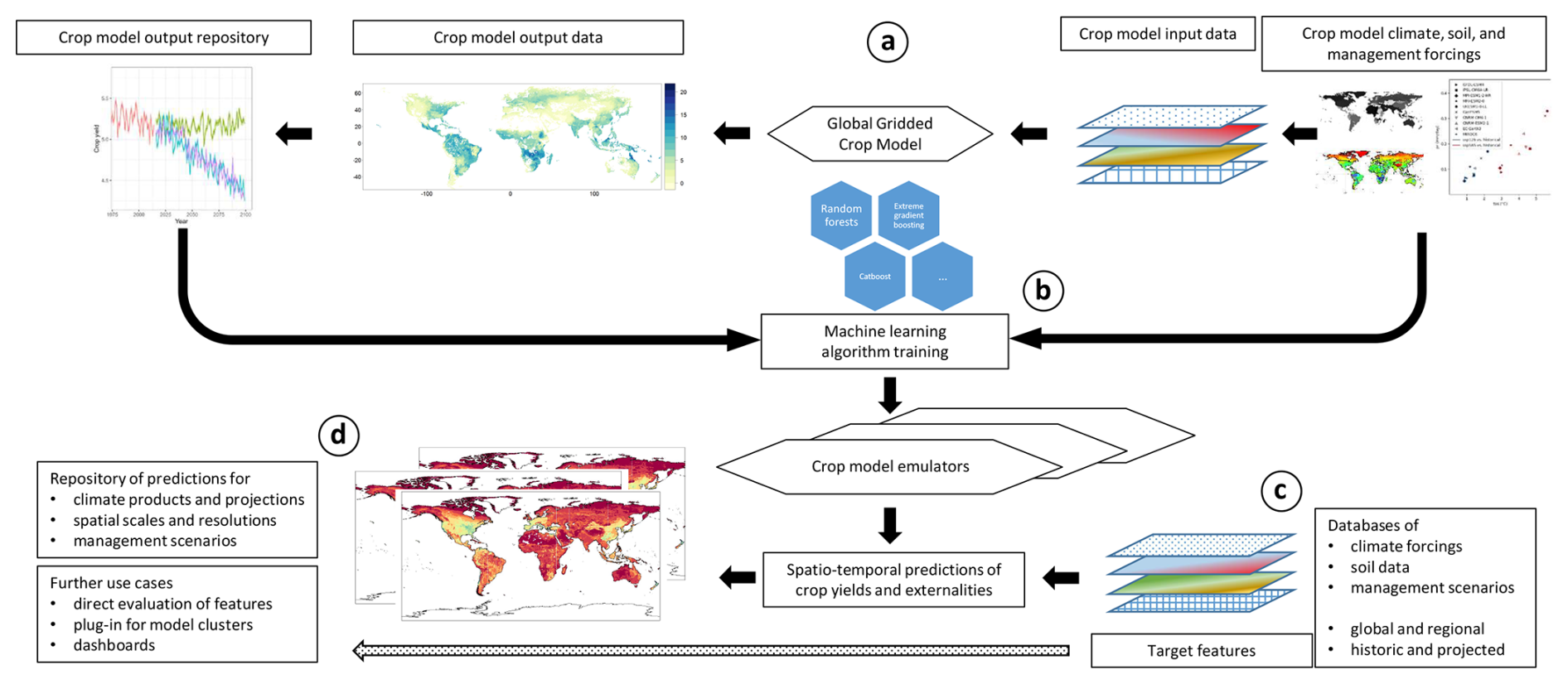
Figure 1 Study design schematic. (a) Global gridded crop model simulations for a specific set of forcing data to generate a training sample for emulators, (b) training of crop model emulators based on machine learning algorithms and the global GGCM training sample, (c) processing of features from target forcings and predictions using emulators from (c), (d) storage and evaluation of predictions and/or optional further use of climate features.

The exemplary application of CROMES herein evaluates in how far emulators that are trained on GGCM simulations for a specific GCM covering the historical time period and three projections along different representative concentration pathways (RCPs; see Sect. 2.9) are skilled to predict crop yields for climate scenarios from other GCMs. Essentially, we perform GGCM simulations using climate forcings from five GCMs, subsequently train emulators for each of these GCMs individually, and benchmark crop yield predictions for the other four GCMs against actual crop model simulations.

While crop nutrient supply can in principle be added to the features, we opt herein to evaluate only predictions for simulations with sufficient nutrient supply to single out the skill of the emulators to capture climate signals.

2.2 Technical design of the emulator pipeline

The code implementation of CROMES is closely aligned with the study design (Sect. 2.1) and detailed in the subsequent sections. CROMES handles the processing of data, feature engineering, training of emulators, and emulator evaluation in four steps:

1. conversion of netCDF climate data to binary files for rapid read access

2. processing of soil, site, crop management, and climate features

3. emulator training

4. emulator application

Implemented features are mostly generic. These include among others growing season aggregates of key climate variables, soil texture, and crop growing season information. More complex approaches are required for the estimation of potential evapotranspiration (PET), which can be based on various methods in crop models (Wartenburger et al., 2018). Herein, we use the Penman-Monteith method that is widely used within GGCMs (Jägermeyr et al., 2021) and has been implemented in the EPIC model as described in (Stockle et al., 1992). We use the CatBoost algorithm for emulator training, a computationally highly efficient algorithm that has been top-ranking in benchmarks (Prokhorenkova et al., 2018) and tested in a wide range of applications (Hancock and Khoshgoftaar, 2020).

2.3 Climate data pre-processing

Climate features are produced for an individual pixel as aggregates over specific time periods (e.g. annual growing season; see Sect. 2.4). In this calculation the whole set of values of each climatic variable needs to be made available to an aggregation function, essentially for the estimation of PET. Therefore, the original set of two-dimensional maps in the netCDF files typically used to supply spatio-temporal climate data has to be converted to a set of vectors, i.e., time series, of individual map pixels for a defined land mask. This conversion of maps to vectors is carried out in a netCDF to binary file translation routine.

The conversion carried out once per climate data set substantially speeds up the subsequent climate feature engineering process. Selecting all climatic values sequentially for each individual map pixel is infeasible due to the large size of the pixel set (here, the ISIMIP 3b cropland mask with 65 797 pixels) and the large number of days (about 36 500 for a 100-year dataset). Together with the number of climatic variables (here six) this leads to about 66 000 × 36 500 × 6 = 14 × 10⁹ selection operations from individual files. As one selection (seek) operation on a state-of-the-art solid-state drive can take more than 0.01 to 0.2 ms, this would result in 14 × 10⁹ × 0.01$/$1000$/$3600$/$24 = 2 to 40 d of processing, assuming that data is not loaded into computer's memory or cached. This bottleneck can be solved in a straightforward manner, if there is sufficient memory available on a user's computer, but the memory consumption would be close to 360 × 720 × 36 500 × 6 × (4 bytes/value) = 210 GB for loading all uncompressed netCDF files into memory. To substantially speed up climate feature processing while avoiding large memory requirements, our implementation carries out a data format conversion through a dedicated routine that is extensively using a small portion of RAM (less than 1 GB) by handling netCDF files individually and producing intermediary binary files. These can subsequently be used for sequential data processing that avoids intensive seek operations or extensive memory use. This allows to (1) reduce running time down to few minutes, (2) avoid dependence on high-end hardware, and (3) supports parallel runs in a high-performance computing environment.

While netCDF files may vary in their configuration, the routines presently implemented in CROMES expect netCDF files compliant with data format conventions used within ISIMIP phase 3b, which are based on NetCDF Climate and Forecast (CF) Metadata Conventions CF-1.6 and a spatial resolution of 0.5° × 0.5°.

2.4 Feature engineering

2.4.1 Summary of included features

Table 1 provides an overview of implemented climate features. The first six rows (TMX to HUR) correspond to raw climate input variables for the EPIC crop growth model that are here used both directly and in the calculation of derived climate features. The latter include growing degree days (GDD; see Sect. 2.4.2), the number of hot degree days (HDD), extreme degree days (EDD), numbers of wet and dry days, and the actual length of the growing season or selected key stages (see below). PET (see Sect. 2.4.3 for details) is used directly and in the calculation of the climatic moisture deficit (CMD) and days with CMD below zero (CMDlt0) as drought indicators. Further outputs of the climate feature module are the individual growing season length (GSL) and the maturity status of the crop at harvest (HUIeopv). CO2trans has a globally uniform annual value.

Table 1 Overview of climate features by climate variable and temporal reference. Actual growing season (AGS) length is dynamically estimated each season (see Sect. 2.4.2). {agg} in the bottom part refers to average (av) or sum (sum) over the respective period. An exemplary feature descriptor would accordingly be TMXavAGS. HUIeopv as an indicator for crop maturity is only output for the whole growing season. CO2trans has an annual value and is hence not aggregated.

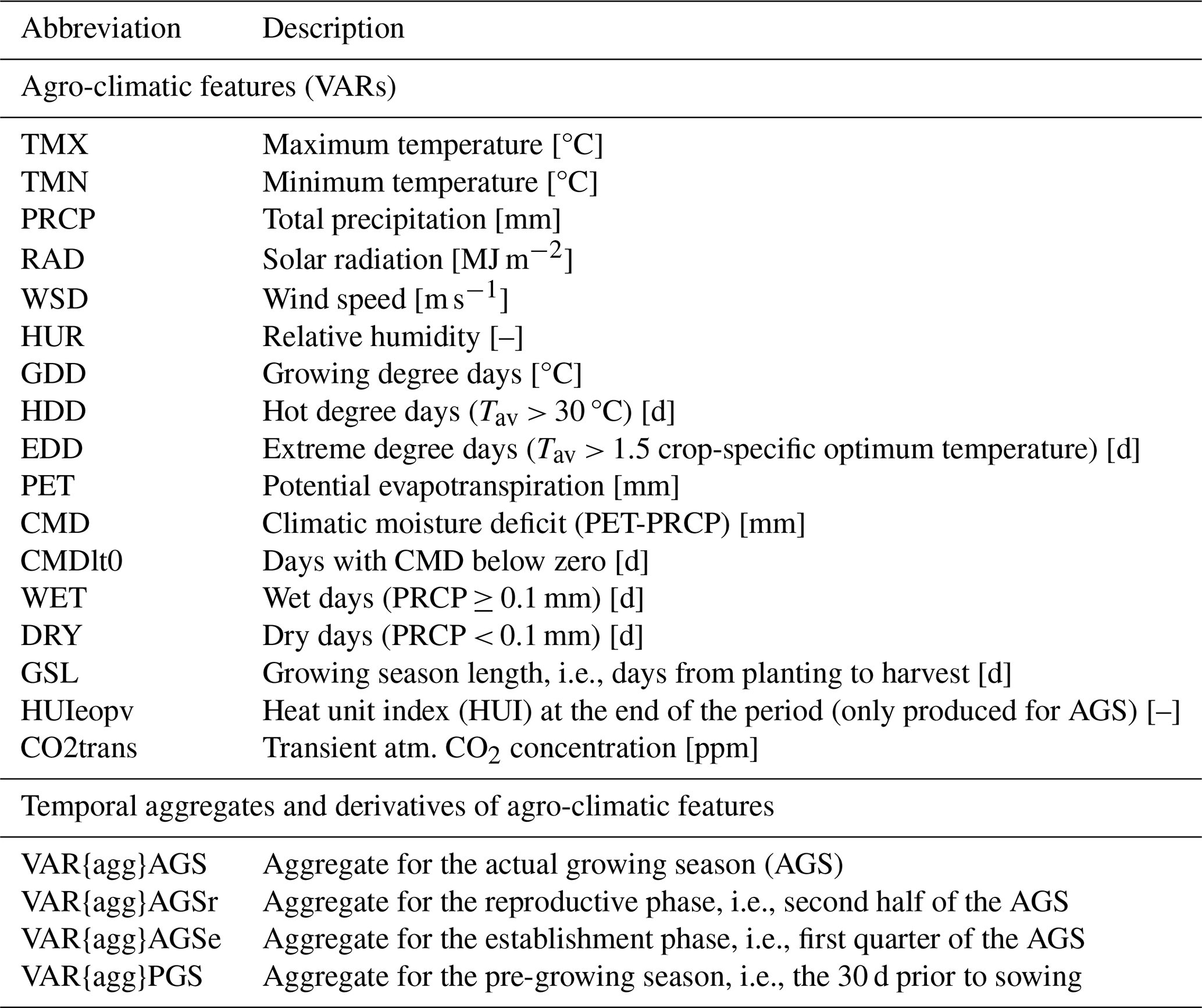
Aggregations are performed (a) for the whole actual growing season (AGS) starting with germination, (b) for the first quarter of the growing season during which the crop emerges (AGSe), (c) for the second half of the growing season – i.e., the reproductive phase during which flowers are prone to water stress (Williams et al., 1989) – (AGSr), and (d) for the 30 d prior to the growing season, during which soil water available for the crop may accumulate (PGS). This breakdown into key growth stages – while also considering growing season totals – serves for improving the information content not only with respect to growth stage-specific crop sensitivities to stresses but also with respect to synchronous or asynchronous manifestation of plant growth limitations such as drought and shading. We use the term actual growing season here to indicate that the climate feature module estimates the crop growth duration for each individual season based on growing degree day (GDD) accumulation as opposed to using a fixed calendar that would not account for earlier (later) maturing of crops in warmer (cooler) years. The estimation of the time periods is further elaborated in Sect. 2.4.2.

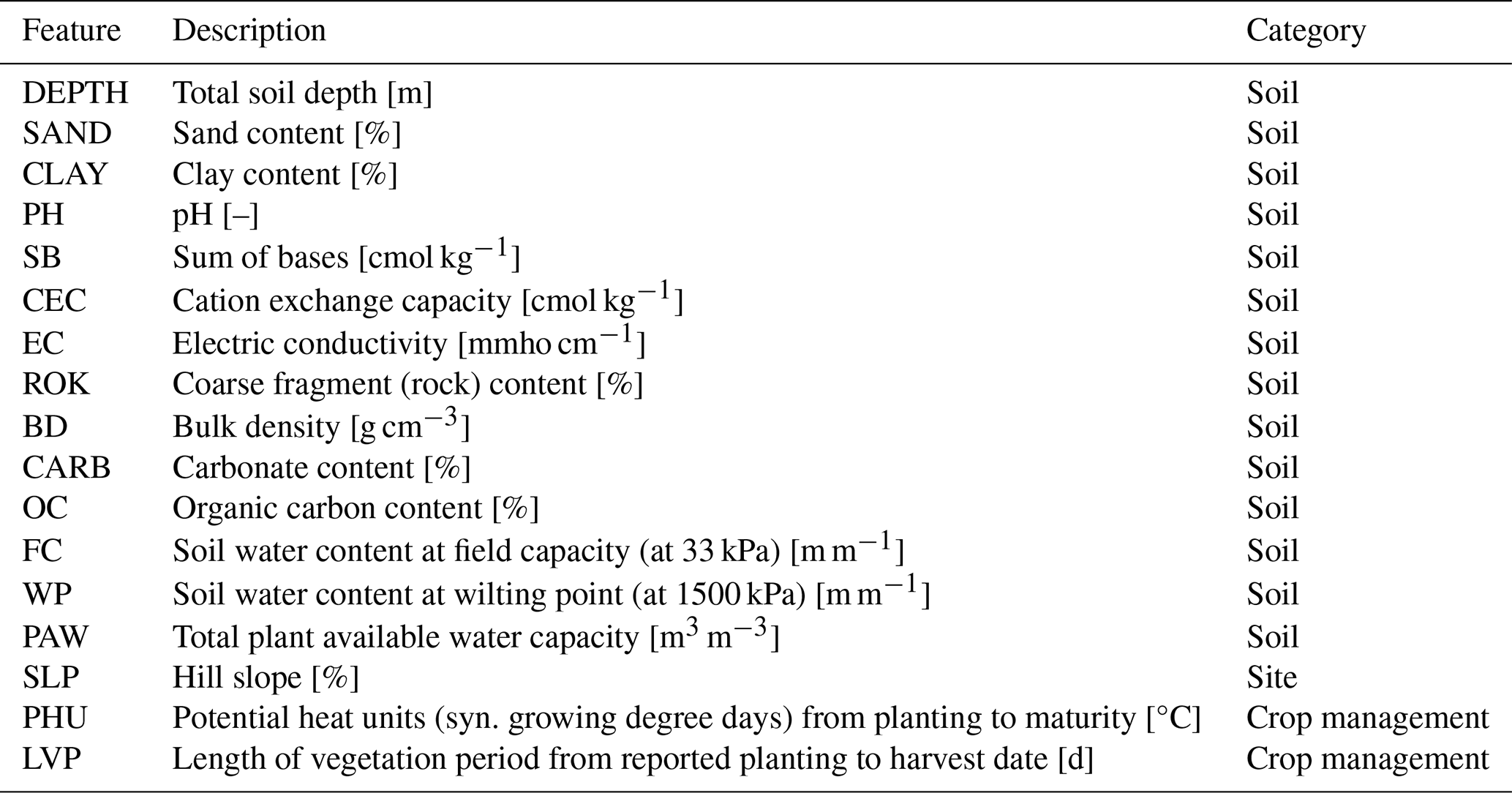
Table 2 shows the non-climatic, temporally static features, essentially soil attributes and slope that impact soil hydrology and root space (see Sect. 2.8). Two crop management parameters are the crop's pixel-specific length of vegetation period (LVP) based on the input planting and harvest dates and the potential heat unit (PHU) requirement.

Table 2 Static soil, site, and crop management features considered in the present setup.

2.4.2 Estimation of growing season length and sub-seasons

The estimation of growing season length is based on GDD accumulation as implemented in the EPIC model and most other GGCMs (Jägermeyr et al., 2021; Müller et al., 2017). Any adjustments can be made in the code or input parameterization that includes parameters for crop-specific base and optimum temperatures.

Earlier crop model emulators and various analytical studies combining crop model simulations and climatic indicators for climate impact estimation have utilized monthly or annual climate features (Blanc, 2017; Folberth et al., 2019; Franke et al., 2020a; Goulart et al., 2023; Sweet et al., 2023). While annual features cannot be expected to capture more than trends in climate, monthly features – typically ordered from planting – at least capture some dynamics within the growing season. Yet, neither of the two considers the effect of earlier (later) crop maturity due to warmer (cooler) than baseline average growing season temperatures. This is one of the main climate impact drivers in crop models (Minoli et al., 2019; Zabel et al., 2021). It determines for example the amount of solar radiation the crop receives for biomass accumulation and whether it is exposed to adverse weather occurring later in the reported growing season. As in the majority of crop models, the progression of crop development from planting to maturity is in CROMES estimated based on the heat unit (HU, syn. growing degree days (GDD)) accumulation approach. That is, on each day i of the growing season daily HU are calculated according to:

$$\begin{array}{}\text{(1)}& {\mathrm{HU}}_i={\displaystyle \frac{T_{max,i}+T_{min,i}}{\mathrm{2}}}-T_{\mathrm{b}},\mathrm{with}{\mathrm{HU}}_i\ge \mathrm{0}\end{array}$$

where T_max [°C] is daily maximum temperature, T_min [°C] is daily minimum temperature, and T_b [°C] is the crop-specific base temperature for growth, here 8 °C for maize. The sum of HU for recent historic average temperatures between reported planting and harvest dates in a location is considered a static cultivar definition termed potential heat units (PHU). Based on input planting dates and PHU, the model estimates the progression of plant phenological development, biomass accumulation, and maturation for each individual growing season. Harvest occurs dynamically after the PHU value is reached (or at a defined cut-off, see below). To normalize plant maturation across locations, a heat unit index (HUI) is used, which is calculated as the cumulative fraction of required PHU reached on day i of the growing season as

$$\begin{array}{}\text{(2)}& {\mathrm{HUI}}_i={\displaystyle \frac{\sum _{k=\mathrm{1}}^i{\mathrm{HU}}_k}{\mathrm{PHU}}}\end{array}$$

The HUI at harvest serves as a feature (HUIeopv) herein to inform whether the crop has reached maturity. Prior to emergence of the crop, an additional amount of germination HU (GMHU) is required for the seed to develop to a seedling, here a GDD sum of 100 °C for maize.

Figure 2 provides an overview of growing season-based climate feature aggregation (incl. pre-growing season (PGS)). The climate feature module first estimates for each growing season based on the input planting date, GMHU, and PHU the germination and maturity dates. If the crop does not mature due to too low growing season temperatures, a cut-off is enforced 21 d after the reported harvest date. Subsequently, climate features are calculated for the whole actual growing season (AGS) and the critical growing season phases for crop establishment (AGSe) and reproductive phase (AGSr). The first occurs from HUI = 0 to HUI = 0.25, the second from HUI = 0.5 to HUI = 1.0 or cut-off date. During the reproductive phase, the crop yield is most sensitive to drought. The PGS is defined as 30d prior to planting, a period that may inform on germination and early growth conditions such as soil humidity.

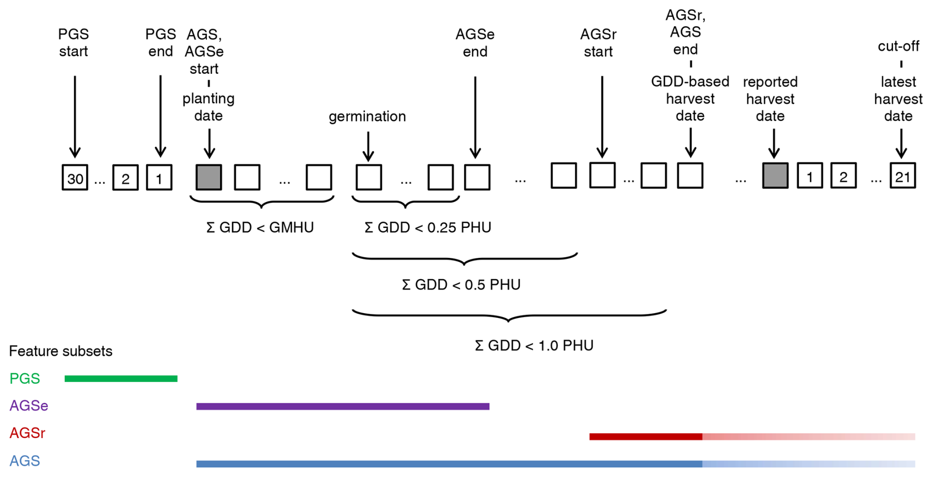
Figure 2 Conceptual definition of the crop growing season and growing season-oriented climate feature subsets. Squared boxes indicate individual days for periods that are universally pre-defined (with numbers) or flexible based on individual input growing season dates and GDD accumulation (empty). PGS = pre-growing season, AGS = actual growing season, AGSe = actual growing season emergence phase (1st quarter), AGSr = actual growing season reproductive phase (2nd half), cut-off = forced growing season cut-off if PHU are not reached 21d after reported harvest date, GDD = growing degree days (syn. heat units), PHU = potential heat units (i.e., GDD estimated for the baseline period as part of cultivar definition). Colored bars in the lower part of the figure indicate the extent of the growing season subsets. The lighter colored extensions at the end of AGS and AGSr indicate that the end of the growing season is either determined by reaching GDD ≥ 1.0 PHU or at the cut-off. The latter serves to avoid overly long growing seasons in cool years where a crop may not reach maturity in autumn and the growing season would hence extend over winter.

2.4.3 Penman-Monteith PET estimation

There are numerous methods for estimating PET employed in GGCMs (Jägermeyr et al., 2021; Liu et al., 2016; Wartenburger et al., 2018) with varying degrees of complexity and input data requirements. The most popular choice is Penman-Monteith (Jägermeyr et al., 2021), which is also implemented in the EPIC crop growth model based on (Stockle et al., 1992). The same approach was followed herein for PET estimation in CROMES.

Penman-Monteith requires all raw climate variables (first six rows in Table 1) as well as information on daily crop height (CHT) and leaf area index (LAI), rendering its estimation considerably complex. The underlying calculations are therefore only provided in abbreviated form and the reader is referred to the above reference and the code for further details. In short, the climate feature module estimates daily progression of CHT and LAI based on HUI and crop-specific parameters, and passes these parameters, daily climate data, and further coefficients (atm. CO₂ concentration, elevation, soil albedo, latitude) to the PET function. Whether or not a crop is growing on a day determines the use of the main equation which is

$$\begin{array}{}\text{(3)}& E_o={\displaystyle \frac{\mathit{\delta }\left(h_o-G\right)+\mathrm{86.7}\mathrm{AD}\left(e_a-e_d\right)/\mathrm{AR}}{\mathrm{HV}\left(\mathit{\delta }+\mathit{\gamma }\right)}}\end{array}$$

if no crop is grown or if a crop grows

$$\begin{array}{}\text{(4)}& E_o={\displaystyle \frac{\mathit{\delta }\left(h_o-G\right)+\mathrm{86.7}\mathrm{AD}\left(e_a-e_d\right)/\mathrm{AR}}{\mathrm{HV}\left(\mathit{\delta }+\mathit{\gamma }\left(\mathrm{1}+\mathrm{CR}/\mathrm{AR}\right)\right)}}\end{array}$$

where AD is the air density [g m⁻³], AR is the aerodynamic resistance for heat and vapor transfer [s m⁻¹], and CR is the canopy resistance for vapor transfer [s m⁻¹], HV is the latent heat of vaporization [MJ kg⁻¹], e_a is saturation vapor pressure [kPa], e_d is actual vapor pressure [kPa], δ is the slope of the saturation vapor pressure curve [kPa °C], G is soil heat flux assumed zero in the model, h_o is net solar radiation [MJ m⁻²], and γ is the psychrometric constant [kPa °C].

2.5 Non-climatic features

Soil features (Table 2) include soil physical and chemical attributes as commonly required by crop models and provided in state-of-the-art data sources such as the one used herein (see Sect. 2.9). Here, we used soil features stored after a spin-up run of the crop model for full consistency with crop model simulations. The first 11 rows of soil features (DEPTH to OC) in Table 2 are raw values, the remainder has been estimated based on routines implemented in the EPIC model (FC, WP, PAW). PHU have been derived as described in the prior sections.

2.6 Emulator training and feature importance

All features, including the target variable crop yield for model training, are eventually merged based on simulation unit IDs or climate grid IDs (see Sect. 2.8). For the demonstration herein, we chose CatBoost, a high-performing algorithm with GPU support that significantly speeds up the training phase (Prokhorenkova et al., 2018). Hyperparameter selection was done using cross-validation (CV) and grid search as implemented in the Python catboost package. This step should be tailored to each specific training and prediction setup. However, this would imply a high resource demand with likely similar outcomes for the datasets used herein. Therefore, we performed the procedure on only one climate dataset, UKESM1-0-LL with ssp585 forcing (see Sect. 2.9).

Provided the abundant data and high dimensionality (60 features), only two hyperparameters were selected for grid-search using 4-fold CV. These are depth of the trees (short depth) in steps of [8, 11, 14] and the maximum number of trees (short iterations) in steps of [400, 800, 1200, 1600]. The default grid-search procedure is implemented in CatBoost as follows: The dataset is split into 80 % training and 20 % test data. For all possible combinations of parameters (points of the grid), a model is fitted on the train dataset. Among the models, the one best performing on the test dataset is selected and sent to CV. Within the above defined grid, the first best model parameters were (14, 1600) achieving a test RMSE equal to 0.4446 t ha⁻¹ (and test-RMSE-mean 0.4470 t ha⁻¹ for 4-fold CV). The second-best model parameters were (14, 1200), test RMSE = 0.4682 t ha⁻¹, followed by (11, 1600) with test RMSE = 0.4871 t ha⁻¹. The experiments demonstrate that there is no overfitting, and results should be close to the lowest feasible generalization error for models fitted using this dataset. Even if a further small increase in accuracy is possible, it may deteriorate performance in emulator applications.

With fixed depth = 14 and iterations = 1600, the remaining training parameters were left to default values. For further emulator training, climate scenarios (i.e., historical and three SSPs; Sect. 2.9) were pooled for each GCM separately and emulators trained on the whole sample as the other four GCMs not used in the training were subsequently used as novel data for benchmarking (see subsequent sections). This setup differs from the more common approach of training machine-learning models on historical data with extensive CV and applying them on future scenarios (Richetti et al., 2023; Sweet et al., 2023). Here, models generalize over scenarios rather than time, and similar data distributions and levels of correlation are expected. To support our assumptions, we provide bootstrapped RMSEs with confidence bounds that show the generalization ability of the model (see Sect. 2.7).

CatBoost provides three approaches to estimate feature importance: Prediction Values Change (PVC), Loss Function Change, and Shapley Additive Explanations (SHAP). The computational complexity of these approaches increases substantially in the same order. For example, computing SHAP values with the Python package SHAP (Lundberg et al., 2020) becomes computationally impractical for our datasets and models without further subsampling at a rate of 0.0001 and lower. PVC in turn is readily available after the training procedure. We hence select herein PVC, which quantifies the average level to which altering a feature value influences the predicted value. PVC importance values are non-negative and normalized so that their sum for all features equals 100.

2.7 Emulator evaluation metrics

In line with earlier studies on crop model emulator development (Blanc, 2017; Franke et al., 2020a; Oyebamiji et al., 2015), we use the root mean square error (RMSE) and linear regression statistics (Pearson's correlation coefficient R², slope, and intercept) to evaluate emulator performance. The first also corresponds to the metric for the loss function in emulator training (see Sect. 2.6). To evaluate the robustness of mean RMSE estimates across the whole sample, we estimate 95 % confidence intervals (CI) bootstrapping 500 subsets of 100 k samples each. We provide all metrics for two sets of benchmark data:

1. We evaluate the performance on the training data itself to show how well the model can fit these training data (Sect. 3.1), which also serves as a reference for evaluations on unseen target data.

2. The main objective of the performance evaluation, however, is the emulators' skill in predicting crop yield simulation outputs for climate projections that have not been used in emulator training (Sect. 3.2). Essentially, we train individual emulators for each of the five GCMs used in this experiment (see Sect. 2.9) and then apply each of these emulators to the remaining four GCMs not used in each emulator's training. This serves as a vast empirical test of how well the emulators perform on unseen climate features while staying within a comparable domain of climate projections.

Evaluations are performed across all individual locations (simulation units) and years as well as for global and sub-continental area-weighted aggregates. For spatial aggregation, crop yields are area-weighted based on the extent of crop- and water management-specific harvested area in each 5 arcmin pixel. Harvested areas were sourced from the SPAM 2010 v2.0 dataset (International Food Policy Research Institute, 2020; Yu et al., 2020). Additional evaluations by climate domains were performed using a dataset of major Koeppen-Geiger climate regions (Beck et al., 2018).

Besides prediction performance, we also approximate the computational time requirements for data pre-processing, crop model simulations, feature processing, and emulator predictions to provide an estimate of speed gain when using emulators. This is done by performing all processing and simulations on a computational cluster with an Oracle ZS5 network storage system and computational nodes equipped with Intel Xeon Gold 2.1 GHz CPUs. All processes are performed on single cores to ensure comparability. An exception is the emulator training, which is done on a GPU (Nvidia RTX A6000) as it would require unreasonably more time on a common CPU.

2.8 Global gridded crop model and simulation setup

EPIC-IIASA (Balkovič et al., 2014) is a GGCM based on the field-scale process-based crop model Environmental Policy Integrated Climate (EPIC) v0810 (Izaurralde et al., 2012; Williams et al., 1989). EPIC-IIASA has been applied extensively in global climate impact studies and has shown good skill in reproducing both historic absolute yields under business-as-usual management and inter-annual yield variability (Balkovič et al., 2013, 2018; Müller et al., 2017). Key processes of the core model EPIC are available from the prior references and summarized in (Folberth et al., 2016).

EPIC-IIASA is based on a 5 arcmin × 5 arcmin spatial grid (equivalent to about 8.3 km × 8.3 km near the equator) for soil characteristics and topography that are aggregated to homogenous response units based on classification of key land surface characteristics (soil, slope, elevation). These are intersected with a 30 arcmin × 30 arcmin climate grid (about 50 km × 50 km near the equator) and national administrative boundaries to define simulation units for each of which the crop model is eventually run (Skalský et al., 2008). Accordingly, simulation units vary in size from 5 arcmin × 5 arcmin to 30 arcmin × 30 arcmin depending on local heterogeneity. Globally, this results in nearly 162 k simulation units within 66 k climate pixels. Out of these, around 151 k simulation units are included here based on general suitability for crop cultivation (i.e., soil present and sufficient temperature).

The setup and parameterization of the EPIC-IIASA GGCM was kept the same as in ISIMIP3b (Jägermeyr et al., 2021) except that we used here sufficient nitrogen (N) fertilizer inputs to focus on climate signals. Following this approach, N is applied automatically by the model as required by the crop to meet its demand for biomass accumulation. The model's application threshold parameter BFT0 was set to 0.99, corresponding to N application if N stress limits crop growth by more than 1 % compared to the potential, the maximum annual input FMX was set to 999 kg N ha⁻¹ yr⁻¹ to ensure that no N stress occurs. We selected maize as a model crop due to its nearly ubiquitous cultivation globally. All simulations assumed rainfed water supply only. The time period for simulations and evaluation is 1980–2099, spanning the historical climate baseline 1980–2014 and projections from 2015–2099. We skip the last year 2100 as outputs are reported by the year of planting (Müller et al., 2017) and no harvest takes place in the last simulation year if the crop is planted in autumn and harvested the following spring.

2.9 Input data

The same raw data were used for both GGCM simulations and emulator training and predictions. Several key input data (soil attributes, growing season dates, climate data), have been provided by the most recent phase 3b of ISIMIP and GGCMI initiative as documented in Jägermeyr et al. (2021). Soil data were originally derived from the Harmonized World Soil Database (FAO et al., 2012) and have been processed for crop land by ISIMIP and GGCMI (Volkholz and Müller, 2020). For the experiment herein, we used soil attributes stored after a spin-up run of EPIC-IIASA, which had been used in the crop model climate impact simulations as well. Slope and elevation had earlier been derived from GTOPO30 (US Geological Survey, 2002).

Climate data were sourced from five global climate models GFDL-ESM4 (Dunne et al., 2020), IPSL-CM6A-LR (Boucher et al., 2020), MPI-ESM1-2-HR (Gutjahr et al., 2019), MRI-ESM2-0 (Yukimoto et al., 2019), and UKESM1-0-LL (Sellar et al., 2019) that span a representative range of equilibrium climate sensitivities (ECS) and transient climate response (TCS). Thereby, MPI-ESM1-2-HR and GFDL-ESM4 are at the low end, MRI-ESM2-0 is in the lower mid-range, and IPSL-CM6A-LR and UKESM1-0-LL present the high end of warming levels at the end of century. For each GCM, we use outputs for the historical time period, as well as the three RCPs 2.6, 7.0, and 8.5. In line with the source climate data combining identifiers for shared socio-economic pathways (SSPs) and RCPs without separators, we refer to the climate scenarios as ssp126 (SSP1 with RCP2.6), ssp370 (SSP3 with RCP7.0), and ssp585 (SSP5 with RCP8.5). Simulations were performed with transient annual atm. CO₂ concentrations corresponding to those of the respective RCPs.

3 Results

3.1 Training metrics

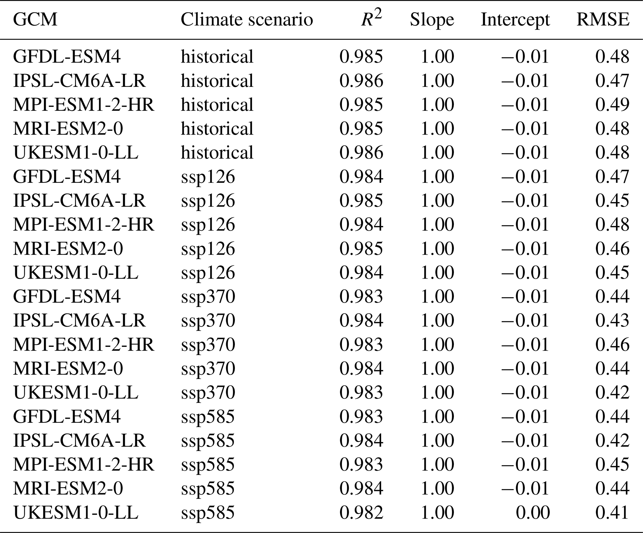
Individual emulators are trained on the pooled climate scenarios of each GCM and subsequently applied to each climate scenario of the same GCM individually. Regression statistics for the training show a near perfect fit with slope and intercept uniformly at 1.00 and −0.01 (except for UKESM1-0-LL with ssp585 forcing at intercept = 0.00) and R² ranging between 0.982 and 0.986 (Table 3). The RMSE varies between 0.41 and 0.49 t ha⁻¹, apparently scaling with absolute yields. These are highest on average during the historical period and lowest under ssp585 (see also Fig. 4). This is more so the case for the two GCMs with high ECS and consequently higher levels of global warming, namely IPSL-CM6A-LR and UKESM1-0-LL (see Sect. 2.9). The 95 % confidence interval width for RMSE on the training data is for all GCMs ≤ 0.01 t ha⁻¹ or ≤ 2 % of the mean RMSE (Table A1 in Appendix A) indicating highly robust results.

Table 3 Regression statistics and RMSE for each emulator trained on all climate scenarios of a specific GCM and applied to each of the source GCM's climate scenarios. Units for intercept and RMSE are t ha⁻¹.

3.2 Prediction performance

3.2.1 Global prediction performance

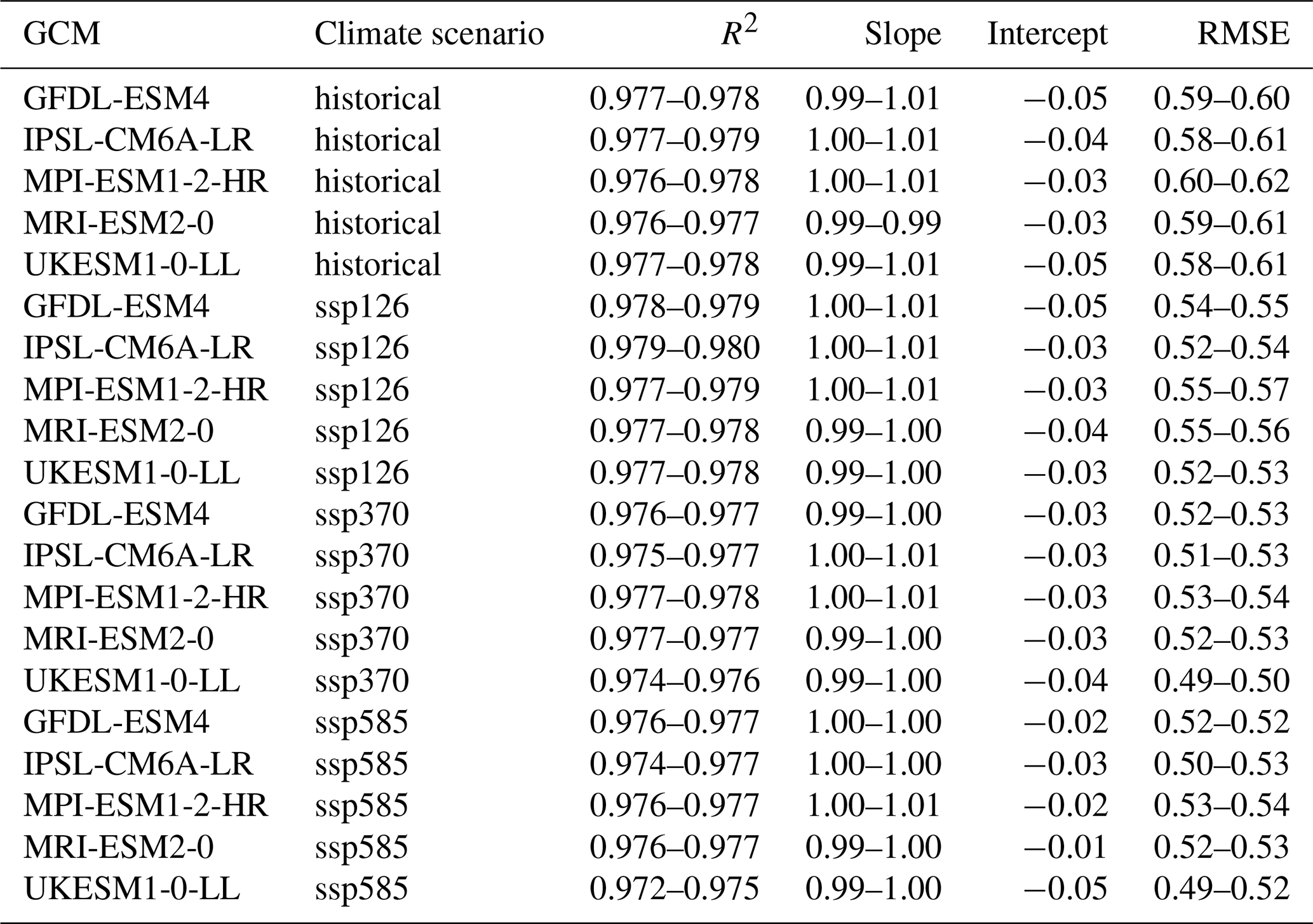
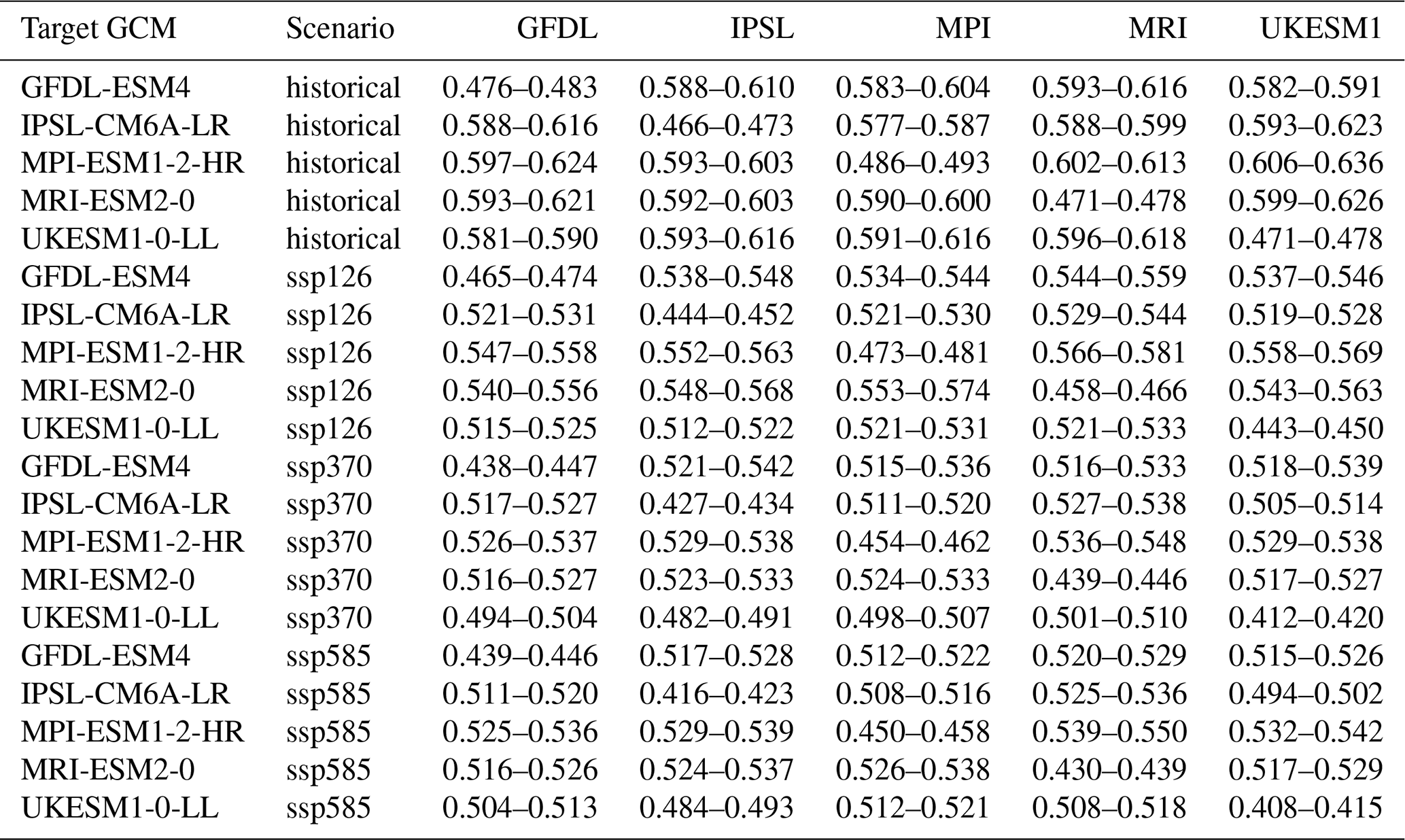
Applying the emulators to climate scenarios from GCMs not seen during training results in only slightly worse regression and RMSE statistics (see Table 4 for overview and Fig. 3 for exemplary visualization). The R² now ranges between 0.974 and 0.980, the slope between 0.99 and 1.01, and the intercept between −0.05 and −0.01. The RMSE is between 0.49 and 0.62 t ha⁻¹. For both latter metrics, larger deviations from the training results occur for the historical time period and in GCMs and scenarios with lower levels of global warming. While the absolute difference is small, the change in RMSE presents an increase by 20 % to 27 % and indicates a slight overfitting of the emulators. The widths of the 95 % confidence intervals are with uniformly ≤ 0.3 t ha⁻¹ (Table A1), corresponding to ≤ 5 % of the mean, as well marginally higher than for the training data but still very low in both absolute and relative terms.

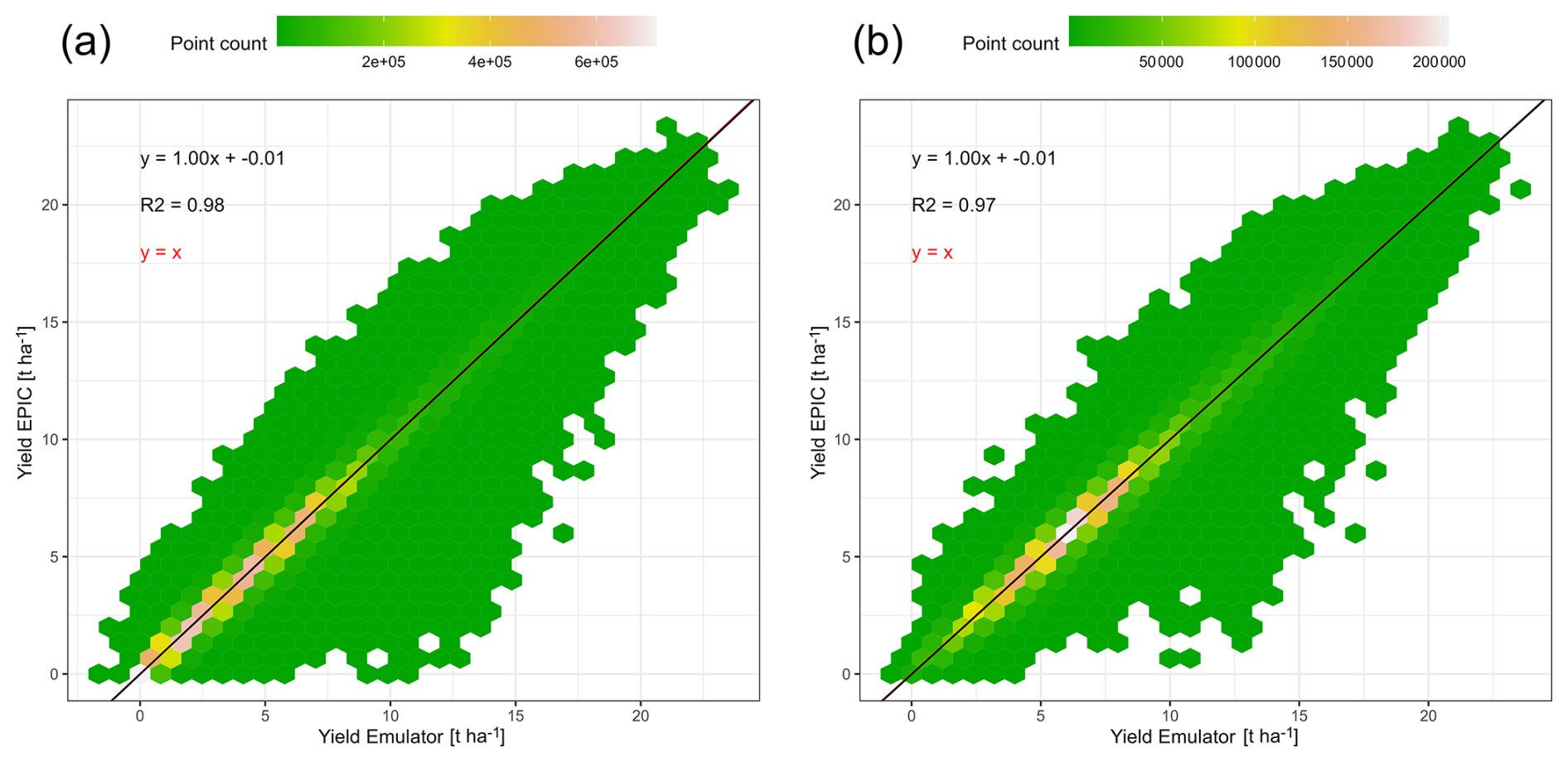
Figure 3 Comparison of exemplary global gridded crop yields for rainfed maize from EPIC-IIASA crop model simulations vs predictions by an emulator that was trained on the GCM IPSL-CM6A-LR and applied to the GCM GFDL-ESM4 for RCP8.5 in both cases with (a) all simulation units and (b) simulation units with >100 ha maize harvested area.

Table 4 Ranges of regression statistics and RMSEs for each emulator trained on a specific GCM and applied to all other GCMs and climate scenario combinations in the demonstration example. Emulators based on the target GCM are excluded. E.g., the first row shows results of predictions for GFDL-ESM4 with historical forcing from the emulators trained on the GCMs IPSL-CM6A-LR, MPI-ESM1-2-HR, MRI-ESM2-0, and UKESM1-0-LL and all climate scenarios (see Methods Sect. 2.9). Units for intercept and RMSE are t ha⁻¹.

Considering only simulation units with rainfed maize harvested area > 100 ha slightly deteriorates the regression statistics (Fig. 3b). Yet, this is at a lower number of samples (n = 36 × 10⁶ compared to n = 127 × 10⁶ in Fig. 3a) and the point density indicates a more pronounced concentration of samples in the yield range 3 to 10 t ha⁻¹ which may affect the regression compared to the wider distribution towards the origin if all pixels are included (Fig. 3a).

Finally, both panels show that predicted yields may include negative values, which occurs in this example for 0.8 % of samples in the whole dataset (minimum −1.4 t ha⁻¹; mean −0.04 t ha⁻¹) and 0.007 % when masking by harvested area (minimum −0.7 t ha⁻¹; mean −0.07 t ha⁻¹). Emulator applications hence need to ensure that predictions are zeroed if valid prediction ranges cannot be defined a priori as is the case for the algorithm employed here.

Global area-weighted mean crop yields show equally a high agreement both between emulator predictions and outputs from the crop model and among the different emulators (Fig. 4). Mean correlation coefficients range between 0.879 and 0.994 with higher values in scenarios with higher levels of warming, i.e. for “hotter” GCMs such as UKESM1-0-LL or IPSL-CM6A-LR and the high concentration pathway ssp585. The lowest values occur at the opposite end of the spectrum (MPI-ESM1-2-HR and MRI-ESM2-0 with ssp126) forcing. Notably, the yield trends may also have an impact here as larger variance facilitates higher R². The ranges of R² values among the emulators applied to the same scenarios are marginal, indicating that the choice of the emulator has little impact on this global metric. Values for RMSE do not show this pattern, while there appears to be a trend towards similar values for the same target GCM (c.f. IPSL-CM6A-LR vs MRI-ESM2-0).

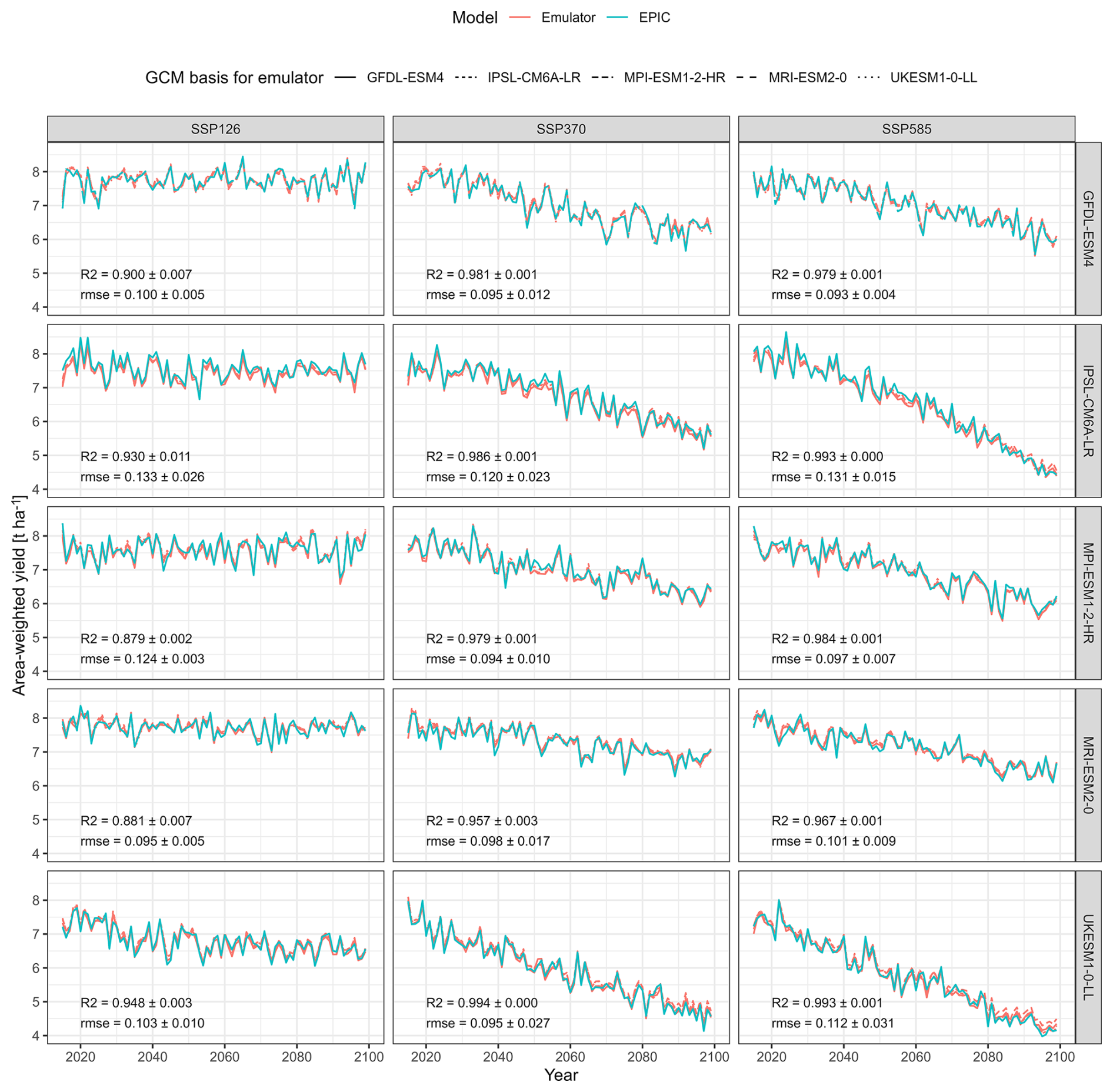
Figure 4 Global annual area-weighted yields of rainfed maize from the GGCM EPIC or predicted by the emulators between the years 2015–2099 for the five priority GCMs used in ISIMIP3b and three SSP-RCP combinations. Each panel shows predictions from four emulators trained on each of the five GCMs except the one providing the target features.

Noticeable deviations occur for specific periods and climate projections, such as the 2050s in ssp370 for IPSL-CM6A-LR and MPI-ESM1-2-HR. In these two instances, there is a high agreement among emulators but not with EPIC simulations. From the 2080s towards the end of century, there is a deviation in yield predictions from the emulator based on MPI-ESM1-2-HR compared to the EPIC simulations for UKESM1-0-LL with ssp585 forcing. In the first case, this may indicate particular climate patterns in the target dataset. In the latter, the high-end warming occurring for this scenario may not be reflected in any of the other scenarios used for emulator training.

3.2.2 Spatial patterns

Aggregating area-weighted crop yields and predictions to geographic macro-regions – exemplary for UKESM1-0-LL with ssp585 forcing – shows a similar pattern as the global performance but with a poorer turnout for both R² and RMSE in regions that have predominantly dry climate, i.e., Northern Africa and to lesser extents Australia and Central Asia with R²=0.713, 0.889, and 0.900, respectively (Fig. 5). Further deviations may at least in part be due to the selection of this high warming scenario.

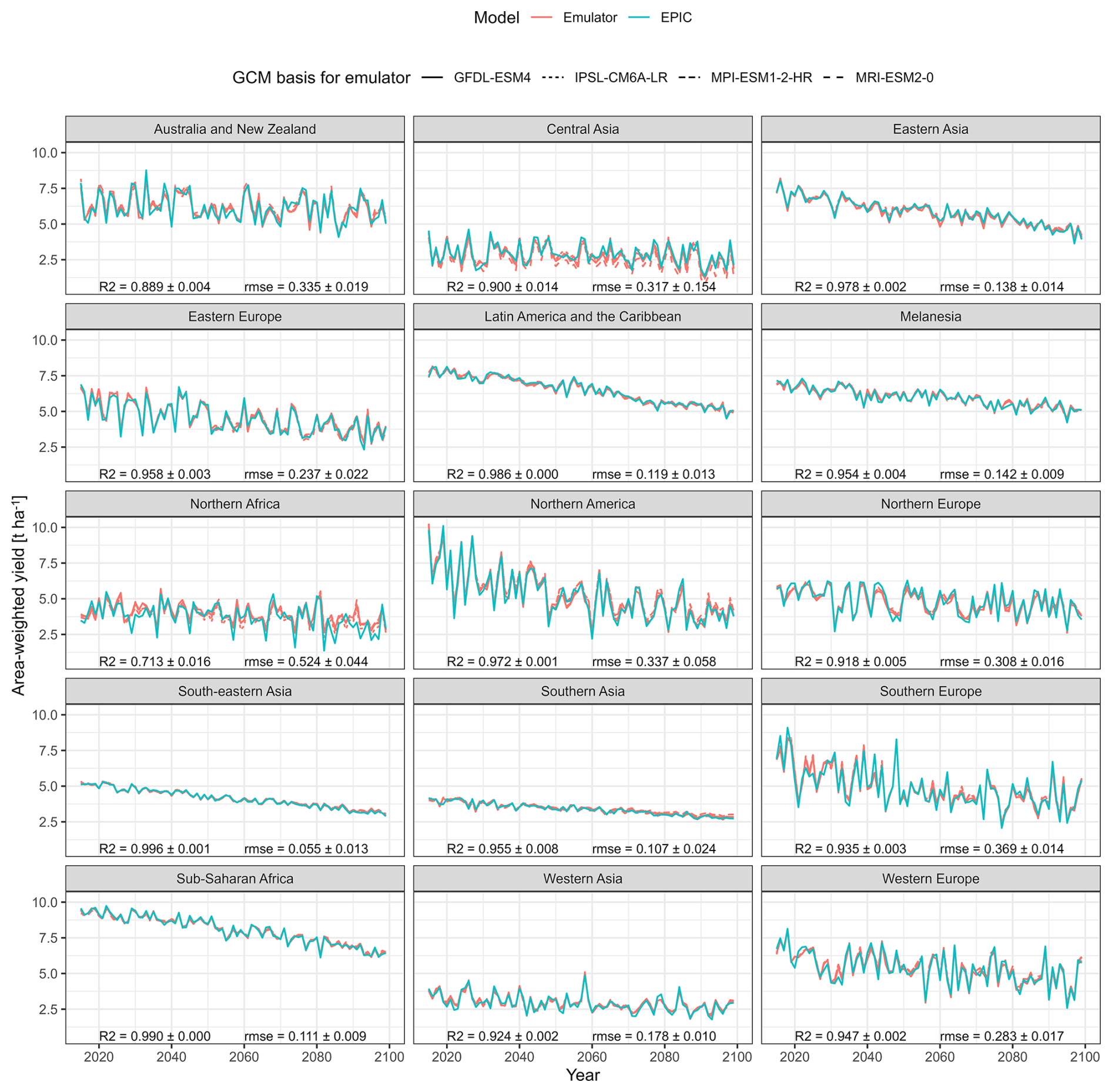
Figure 5 Same as Fig. 4 but for 15 macro regions and target climate dataset UKESM1-0-LL with SSP585 forcing only.

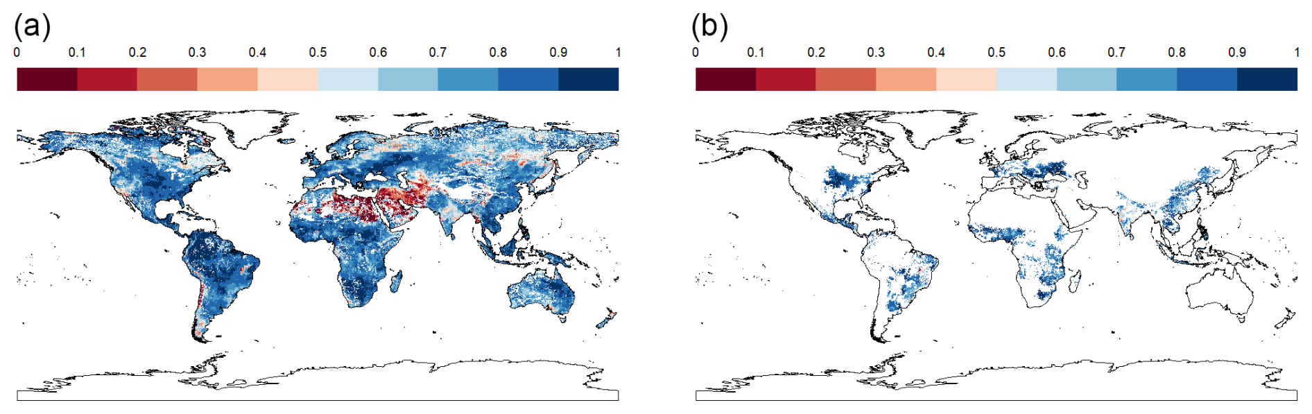
Figure 6 R² of regressions between simulated and predicted rainfed maize yields over 85 years per pixel (i.e., simulation unit) exemplary shown for an emulator based on IPSL-CM6A-LR and applied to GFDL-ESM4 with SSP3-70 forcing for (a) all land mask pixels and (b) pixels with >100 ha harvested area.

Within individual simulation units mapped to 5 arcmin × 5 arcmin pixels, high R² values dominate as well (Fig. 6). These are mixed with very poor outcomes if the whole land mask is considered (Fig. 6a) compared to masking by relevant cultivation regions (Fig. 6b). In the first case, the median R² is 0.794, in the latter case 0.847. Hotspots for poor outcomes are arid regions – especially of the Sahel zone and West Asia – where permanently dry conditions cause constantly low yields with little variability. This also affects the outcomes of regression metrics.

These visual interpretations are supported by density plots of R² per Koeppen-Geiger region – major global climate domains – for the whole land (Fig. A1 in the Appendix) or pixels with maize harvested area > 100 ha (Fig. A2). The first shows that a comparably high tail occurs in (semi-)arid climates and a flat distribution is found for polar climates. Both present challenging environments for agriculture and in the latter case have hardly harvested areas. Accordingly, when removing pixels with marginal harvested areas, the distributions across all climates shift towards higher R² values. The higher performance in pixels with larger harvested areas is reinforced by Fig. A3 displaying R² densities within harvested area bins. The highest tail towards low values is again found for pixels with areas < 10 ha, whereas pixels with very large harvested areas (>1000 ha) have hardly R² values of less than 0.5.

3.3 Feature importance

The importance of individual features shows overall good agreement among the emulators trained on different GCMs with slight variations (Table 5). While the top 10 features ranked by median importance are quite consistent, the agreement tends to decrease with decreasing importance of the features. The uniformly most important feature is the sum of shortwave solar radiation over the growing season (RADsumAGS), a direct aggregate of the photosynthetically active energy received by the crop. This is followed by the growing season precipitation sum (PRCPsumAGS). CMDlt0sumAGS, the number of days with a climatic moisture deficit, presents a drought indicator with similar ranking. Already beyond these three top ranking features, the numeric difference among prediction value change (PVC) outcomes is less discernible and shows a transient decline.

Table 5 Feature importance for the 20 overall top-ranking features out of 60 features measured as prediction value change (PVC; see Sect. 2.6). Median importance is the median of feature importance estimated for each of five individual emulators based on each of the GCMs.

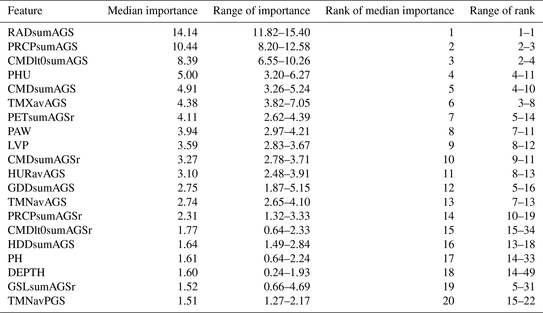
Notably, most of the climate features present in the top 20 refer to growing season aggregates, followed by drought-related features for the reproductive phase (PETsumAGSr, CMDsumAGSr, PRCPsumAGSr, CMDlt0sumAGSr), during which flowering and consequently yield formation is most sensitive to water deficit. Only one feature refers to the pre-growing season period (PGS), the average minimum daily temperature (TMNavPGS), which is not straightforward to interpret.

Non-climatic features include most importantly the crop's heat unit requirement (PHU), a spatially explicit cultivar constant, the closely related length of vegetation period (LVP), and the soil features PAW, PH, and DEPTH. While the first and the last of these relate to soil water storage and therefore modulate water deficit in interaction with weather, pH has typically little impact in the crop model and may hence be correlated with other features.

3.4 Computational performance

As time gain is a key advantage of emulators, we provide a rough estimate of time required for key tasks within the modelling and data processing chains of both approaches – EPIC simulations and emulator training and predictions – to allow for basic contextualization (Fig. 7), while actual performance in individual applications will depend on the computational infrastructure in place and its load. In the setup used herein, both approaches require first a conversion of netCDF files to binary files that provide substantially faster read access. This takes about 0.5 h. Further production of daily weather files for the EPIC model – individual text files for each pixel – takes approx. 2 h. The largest time requirement occurs for the EPIC simulation itself, which here takes 12 h but can vary on the shared cluster between 6 and 18 h on a single core. The crop model produces single output files for each simulation unit from which the extraction of outputs to a compilation file requires 1h. Once a climate dataset has been processed, only the last two steps crop model run and post-processing are required for each simulation.

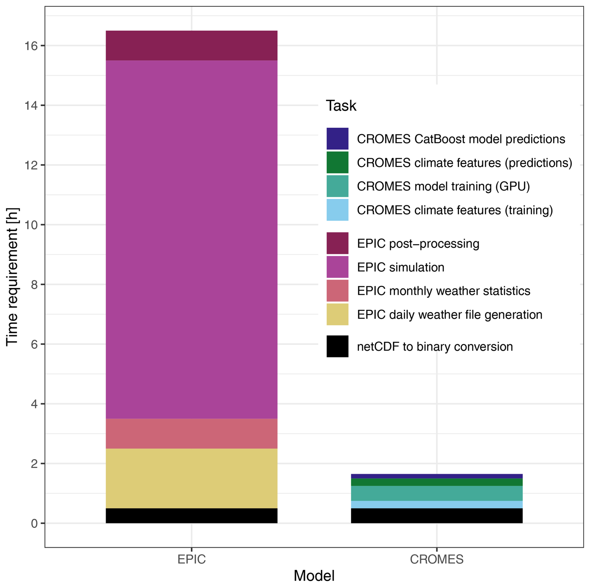
Figure 7 Time requirement for key tasks required to produce global crop model simulations with EPIC or crop yield predictions with CROMES. Some tasks only have to be performed once, essentially the bottom three of the legend or those relating to CROMES emulator training, depending on the specific purpose. The numbers shown here are therefore primarily for illustrative purposes.

Within the CROMES pipeline, generation of climate features for one climate scenario for emulator training or predictions requires about 0.25 h. Model training on a GPU using the CatBoost algorithm requires 0.5 h and predictions, i.e., the combination of climate and other features with subsequent evaluation of the trained algorithm on the feature set, about 0.15 h. Once an emulator has been trained, again only the last two steps are required, i.e., processing of climate features for a target dataset and evaluation of the emulator over the combined feature set.

In total, the emulator provides a speed improvement of at least an order of magnitude, regardless of whether the whole computational chain is considered or only the last two steps producing the actual outputs.

4 Discussion

In principle, model emulators or meta-models present a trade in higher speed for less accuracy. Our evaluation of the CROMES pipeline for an exemplary application highlights that a substantial speed gain is in fact feasible at a comparably low cost in accuracy with most benchmark indicators pointing to a near perfect fit. The lowest agreement between predictions and crop yield simulations occurs in regions with predominantly arid climate where the aggregation of daily weather to climate features potentially fails to capture the effects of timing and volume of precipitation events. These can markedly affect crop yields as do interactions between temperature, atmospheric moisture deficit, and water availability (Schauberger et al., 2017). Yet, rainfed agriculture is typically of limited importance in such regions and the constantly low crop yields pose a challenge to achieving a good regression fit for the global emulator while the absolute error can be considered minor. Overall, the performance of an emulator will need to be evaluated on an application case basis and training routines may need to be adjusted for specific target regions or applications to obtain best results for a specific context. For example, where farming in semi-arid environments or other low-yielding regions is in the focus, the selection of training samples should be tailored to such regions to ensure that the algorithm is not geared towards a mean response that covers a variety of climates where semi-arid conditions present a particular niche. Vice versa, when focusing on breadbasket failures, users may sample such typically high-yielding agro-climatic regions specifically. In the demonstration case herein, that is tailored towards evaluation for broader coverage of global climate projections, we selected accordingly all pixels globally.

To the authors' best knowledge, complex machine-learning algorithms have not been applied prior to train emulators for a GGCM using opportunistic training samples, i.e. data that are readily available from earlier experiments. The performance achieved herein is hence not straightforward to compare to that found in earlier studies. Most recently, Sweet et al. (2023) evaluated CV strategies for training machine-learning algorithms to predict crop yields from GGCMs. They reported a maximum R² of 0.82 on the training set and far lower values around 0.4 on holdout data. However, their application case covered only the historic period and focused on holdout years and regions, which may be more challenging to capture than multi-year and -location climate change projections as herein. Yet, they also assumed static growing season lengths, which does not reflect the conceptualization of plant maturation typical in crop models and loses information on the weather the crop is actually exposed to (see also next paragraph). Rather than a CV, we performed here a bootstrapping of emulator predictions to quantify 95 % CIs for RMSE and found robust results for both our training and application of emulators. Oyebamiji et al. (2015) developed a similar emulator approach as the one herein but using various regression methods and with the objective of predicting changes in decadal mean crop yields based on changes in climate features over the four meteorological seasons. Applied to an older version of the GGCM LPJmL (Bondeau et al., 2007), they found an agreement with R² = 0.72 to 0.86 for unseen climate projections combining RCPs 4.5 and 8.5. Similarly, Blanc (2017) trained statistical emulators for crop yield changes under climate change based on various regression models for several GGCMs and samples from climate impact projections using monthly and meteorological seasonal climate features. This resulted in an R² of 0.43 to 0.78 for multi-year average yield changes depending on the GGCM with R² 0.48 to 0.56 for an EPIC-based GGCM GEPIC. Finally, Franke et al. (2020b) trained GGCM emulators using pixel-specific polynomials for a range GGCMs that had simulated a structured training sample with systematic changes in temperature, precipitation, CO2, and fertilizer application. Applied to an exemplary climate change projection (HadGEM2-ES with RCP8.5) using annual shifters in climate features this resulted in RMSE of 0.9 to 2.7 and 1.8 to 2.4 t ha⁻¹ for two EPIC-based GGCMs compared to herein R² = 0.97 to 0.98 and RMSE = 0.50 to 0.66 on holdout data.

We expect that feature engineering is the key determinant for the high accuracy of crop yield predictions achieved herein, also compared to past research. As outlined above, earlier studies developing emulators or similar hybrid crop modelling tools employed fixed seasonal, monthly, or annual aggregates of climate variables (Blanc, 2017; Folberth et al., 2019; Franke et al., 2020a; Goulart et al., 2023; Oyebamiji et al., 2015; Sweet et al., 2023). These provide basic information on the weather a crop is exposed to in a specific year but neglect that crop maturity is driven by temperatures, represented as GDD accumulation in the vast majority of (global) crop models (Jägermeyr et al., 2021). In fact, keeping the growing season length constant over time under global warming is a common scenario for cultivar adaptation in crop modelling studies (Franke et al., 2020b; Minoli et al., 2019; Zabel et al., 2021). Following the concept of GDD accumulation, CROMES dynamically estimates the actual length of each growing season and its sub-phases after planting. This has earlier been found to be a key determinant of crop yields in GGCMs, especially under high levels of global warming. Essentially, crops mature earlier and have less time for biomass accumulation but may simultaneously not be affected by adverse weather events later in the year (Zabel et al., 2021). A systematic comparison of different feature engineering approaches, however, is beyond the scope of this study and should be subject of a dedicated intercomparison exercise as is common within the crop modelling community for process-based types of models.

Computational speed is challenging to compare between emulators and GGCMs (see Sect. 3.4) and even more so among different studies. These may cover varying GGCMs with highly diverse computational demands or use publicly available training data that do not provide this information. Herein, we estimate a speed gain of conservatively an order of magnitude. Oyebamiji et al. (2015) estimate a speed gain by a factor of 60 for their LPJmL emulator, yet without further specifications of considered steps in the modelling chain. Essentially, in both cases the time requirement decreases from hours to minutes. Based on our results, the largest gain in computational speed is achieved if an emulator is applied for comprehensive scenario analyses, e.g., across large sets of climate projections, which requires a large number of repeated runs of the same emulator.

5 Conclusions and outlook

We expect the crop model emulator pipeline presented herein to bear great potential in various applications including complex climate impact modelling clusters or comprehensive scenario analyses across large climate ensembles and at high spatial resolutions. For such applications computational efficiency is a key advantage and the loss of information compared to the gain in speed achieved herein indicates that outcomes can be considered robust as long as predictors are part of the training domain. Quantifying this validity domain remains a prevailing issue in machine learning and will have to be characterized on a case-by-case basis until robust methods are developed. This will be an important subject for future research. Meanwhile, compared to static emulators CROMES allows for continuous updating of training data such as for the next generation of CMIP7 climate projections, with new GGCM versions, or for applications with very specific feature domains such as global cooling scenarios from geoengineering or nuclear winter. Thereby, no tailored crop model simulations are required for training as long as data from existing experiments are within the application domain and users of the emulator pipeline do not require specific expertise in crop model setups and applications.

Beyond the crop model emulation, we expect CROMES to be useful in two ways: (a) as the input data are quite generic, CROMES can also be used to efficiently train machine learning models on observations to develop observation-based machine-learning crop models; and (b) the climate features as an intermediary product of the pipeline allow for comprehensive analyses of growing season climate itself.

Appendix A

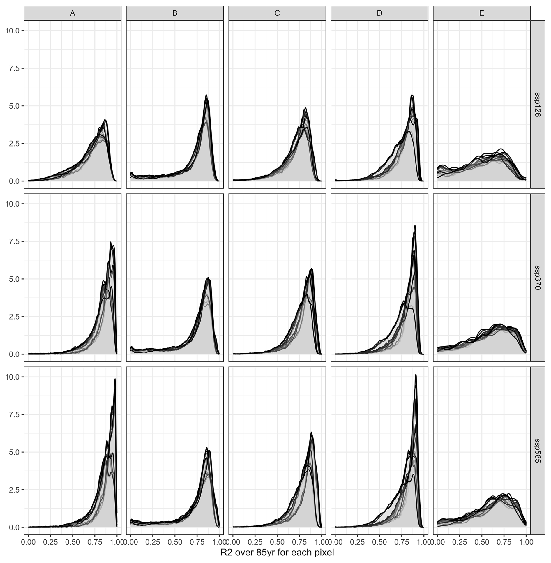
Figure A1 Density of R² per pixel over 85 years for three SSPs (rows) and across five major Koeppen Geiger climate regions (columns). A = tropical, B = (semi-)arid, C = temperate, D = cold, E = polar. Each panel shows 20 plots, applying each emulator trained on one of the five GCMs to the four GCMs not used in its training.

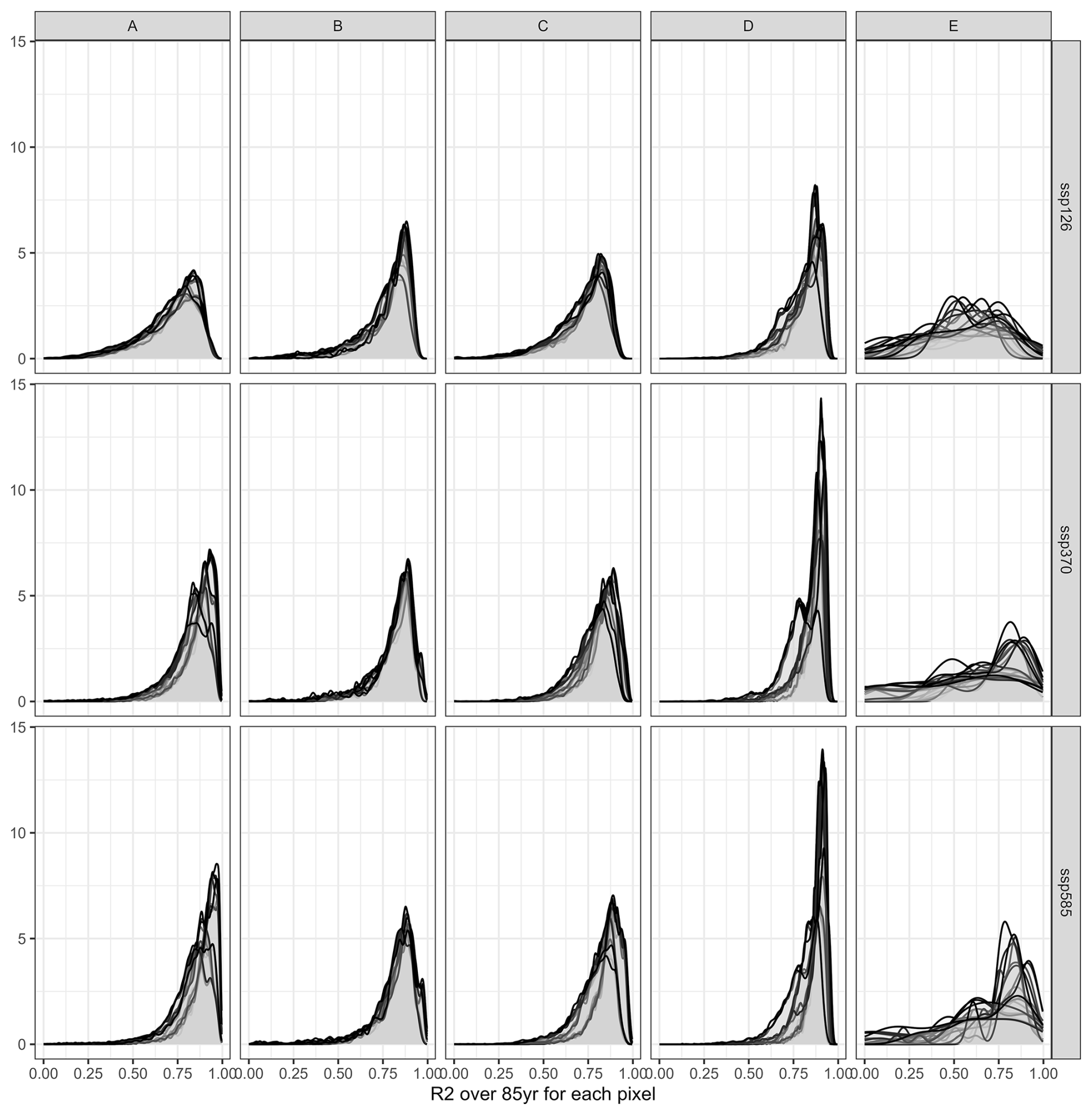
Figure A2 Same as Fig. A1 but showing only pixels with rainfed maize harvested area > 100 ha.

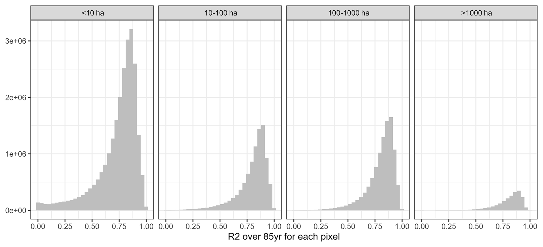
Figure A3 Density of R² per pixel over 85 years for four bins of rainfed maize harvested areas (panels). Data are pooled from applying each emulator trained on one of the five GCMs to the four GCMs not used in its training across all three SSPs.

Table A1 Confidence intervals (CI) for RMSE [t ha⁻¹] estimated through bootstrapping (500 × 100 k samples) for each emulator based on an individual GCM (columns with short GCM name) and applied to each target GCM (rows). Where training and target GCM are identical, the CI corresponds to values shown in Table 3. Where GCMs differ, CIs refer to results shown in Table 4.