flat10MIP: an emissions-driven experiment to diagnose the climate response to positive, zero and negative CO₂ emissions

The proportionality between global mean temperature and cumulative emissions of CO₂ predicted in Earth system models (ESMs) is the foundation of carbon budgeting frameworks. Deviations from this behavior could impact estimates of required net-zero timings and negative emissions requirements to meet the Paris Agreement climate targets. However, existing ESM diagnostic experiments do not allow for direct estimation of these deviations as a function of defined emissions pathways. Here, we perform a set of climate model diagnostic experiments for the assessment of transient climate response to cumulative CO₂ emissions (TCRE), the Zero Emissions Commitment (ZEC), and climate reversibility metrics in an emissions-driven framework. The emissions-driven experiments provide consistent independent variables simplifying simulation, analysis and interpretation, with emissions rates more comparable to recent levels than existing protocols using model-specific compatible emissions from the CMIP DECK 1pctCO2 experiment, where emissions rates tend to increase during the experiment, such that at the time of CO₂ doubling in year 70, emissions are much greater than present-day values. A base experiment, “esm-flat10”, has constant emissions of CO₂ of 10 GtC per year (near-present-day values), and initial results show that the TCRE estimated in this experiment is about 0.1 K less than that obtained using 1pctCO2. A subset of ESMs exhibit land carbon sinks that saturate during this experiment. A branch experiment, esm-flat10-zec, illustrates that both positive and negative ZEC effects are less pronounced under esm-flat10 than under 1pctCO2 – the magnitude of ZEC50 in ESMs is, on average, reduced by 30 % compared with 1pctCO2 branch experiments. A final experiment, esm-flat10-cdr, assesses climate reversibility under negative emissions, where we find that peak warming may occur before or after net zero and that the asymmetry in temperature at a given level of cumulative emissions between the positive and negative emissions phases is well described by ZEC in most models. Further, we find that existing probabilistic simple climate model (SCM) ensembles tend to overestimate temperature reversibility compared with ESMs, highlighting the need for additional constraints. We propose a set of climate diagnostic indicators to quantify various aspects of climate reversibility. These experiments were suggested as potential candidates in CMIP7 and have since been adopted as “fast track” simulations.

1 Introduction

The concept of proportionality of global mean temperatures to cumulative carbon dioxide emissions is central to carbon budgeting frameworks and net-zero commitments (Rogelj et al., 2019b). The relationship has its origins in the recognition of a robust linear relationship in Earth system model simulations (Allen et al., 2009; Matthews et al., 2009; Zickfeld et al., 2009) and observations (Gillett et al., 2013) between the global mean temperature change and the cumulative amount of CO₂ released into the atmosphere, the slope of which we refer to as the transient climate response to cumulative emissions (TCRE) – the change in global mean temperature per trillion tonnes of carbon emitted into the atmosphere. TCRE offers a powerful, simplified lens for climate policy applications, allowing policymakers to directly equate emission budgets to projected warming levels (Lamboll et al., 2023; Rogelj et al., 2019b) and to gauge the relative impact of different emissions trajectories over time (MacDougall, 2015).

For a simulation in which temperature changes are driven by CO₂ alone,

$$\begin{array}{}\text{(1)}& \mathrm{TCRE}={\displaystyle \frac{\mathrm{\Delta }T\left(t\right)}{I_{\mathrm{em}}\left(\mathrm{t}\right)}},\end{array}$$

where ΔT(t) and I_em(t) are the temperature change and cumulative emissions at time t, respectively. For climate models, TCRE is generally calculated using results from a concentration-driven simulation 1pctCO2, where CO₂ concentrations are prescribed and ramped up exponentially at a rate of 1 % per year. In assessments (IPCC, 2023c), the TCRE is nominally computed in year 70, when concentrations have approximately doubled:

$${\mathrm{TCRE}}_{\mathrm{1}\mathrm{pctCO}\mathrm{2}}={\displaystyle \frac{\mathrm{\Delta }T\left(\mathrm{70}\right)}{I_{\mathrm{em}}\left(\mathrm{70}\right)}}=\left({\displaystyle \frac{\mathrm{\Delta }T\left(\mathrm{70}\right)}{I_{\mathrm{atmos}}\left(\mathrm{70}\right)}}\right)\left({\displaystyle \frac{I_{\mathrm{atmos}}\left(\mathrm{70}\right)}{I_{\mathrm{em}}\left(\mathrm{70}\right)}}\right),$$

where I_atmos(70) is the additional carbon in the atmosphere and ΔT(70) is the transient climate response (TCR, in practice calculated as the average over years 60–80). $\frac{I_{\mathrm{atmos}}\left(\mathrm{70}\right)}{I_{\mathrm{em}}\left(\mathrm{70}\right)}$ is the cumulative airborne fraction, the proportion of cumulative emissions which remain in the atmosphere.

In order to constrain compatible carbon emissions budgets for certain warming levels, historical human-induced warming must be calculated, along with some additional corrections (Rogelj et al., 2019b). Firstly, the temperature impact of present and future non-CO₂ emissions must be incorporated, either by assuming a ratio of future CO₂ and non-CO₂ emissions (Damon Matthews et al., 2021; Leach et al., 2018; Millar and Friedlingstein, 2018), by subtracting an estimate of non-CO₂ warming (Lamboll et al., 2023), or by defining a TCRE based on cumulative CO₂- forcing-equivalent emissions (Jenkins et al., 2021).

Secondly, any potential further carbon-induced warming after net zero has been achieved introduces additional uncertainty in remaining carbon budgets calculated using TCRE (Nicholls et al., 2020). This behavior has been characterized by the Zero Emissions Commitment (ZEC) (IPCC, 2023c; Lamboll et al., 2023). Definitions of ZEC are, to date, primarily informed by the ZECMIP CMIP6 experiment (Jones et al., 2019), which is based on an abrupt cessation of emissions branching from the 1pctCO2 experiment when 1000 PgC of CO₂ emissions have been diagnosed, where the notation ZECn corresponds to the warming n years after the cessation of emissions (MacDougall et al., 2020). ZEC50 and ZEC90 are thus the temperature change 50 and 90 years after the cessation of emissions, respectively. This experiment was performed by a coordinated set of Earth system models and intermediate complexity models, which led to the finding that ZEC had the potential to be either positive or negative (MacDougall et al., 2020) with a best estimate near zero.

ZECMIP experiments were designed this way to ensure consistency of ZEC and TCRE at the same point, but they do, however, have a number of limitations. Firstly, 1pctCO2 is a prescribed concentration trajectory for atmospheric CO₂, and compatible emissions are computed as a residual term, such that each climate model has a different emissions trajectory. This poses two issues for using the run as a basis for the assessment of ZEC. Firstly, each model follows its own pathway of (implied) emissions in such experiments, obfuscating the relationship between model and ZEC response. Secondly, the compatible emissions profile in 1pctCO2 grows throughout the experiment, with the burden of cumulative emissions weighted towards the end of the experiment (Sanderson et al., 2024 and Fig. 6), whereas contemporary emissions are closer to flat (since about 2012).

Alternative frameworks have been proposed to provide a less scenario-dependent formulation for ZEC. Consideration of linear pulse-response models of the climate shows that cumulative emissions proportionality is an expected first-order response but that second-order terms allow for further temperature changes after emissions have ceased (Avakumović, 2024; Jenkins et al., 2022). This second-order behavior can be approximated by the rate of adjustment to zero emissions, or RAZE, which defines the fractional change in CO₂-induced warming after CO₂ emissions cease (Jenkins et al., 2022). In this approximation (valid for decadal timescales following net zero), RAZE can be related to ZEC for a given scenario as

$${\mathrm{ZEC}}_H=I_{\mathrm{em}}(t=t_{\text{net-zero}})\left(\mathrm{TCRE}\right)\left(\mathrm{RAZE}\right)\left(H\right),$$

where ZEC_H is the warming H years after net zero and I_em(t=t_{net zero}) is the cumulative emissions at the time of net zero. In this framing, a linear estimate of the warming rate after net zero, if emissions are held at net zero, is given by I_em(t=t_{net zero})(TCRE)(RAZE).

In addition, no experiment within prior CMIP efforts has been designed to robustly understand the degree of asymmetry in the climate response to positive followed by negative CO₂ emissions. The compatible emissions from the 1pctCO2-cdr concentration reversal experiment used in CDRMIP (Asaadi et al., 2024) are both asymmetric in time, between the positive and negative emissions periods, and have a large discontinuity of roughly 50 Pg C yr⁻¹ (Koven et al., 2023) at the point of reversal from increasing to decreasing CO₂ concentrations. Secondly, the lagged effects of the positive emission phase can complicate assessment of the response to negative emissions (Chimuka et al., 2023; Koven et al., 2023; Zickfeld et al., 2016).

These confounding effects inhibit a clear diagnosis of whether and how the general climate response to negative emissions differs from the climate response to positive emissions (MacDougall, 2019). An idealized CMIP experiment that allows for a continuous transition from positive to negative emissions, and one that is symmetric in time (so that any asymmetries that arise are driven by the coupled carbon–climate response itself), improves on this status quo (though the separation of lagged effects remains a challenge).

Here, we propose a compact set of experiments uniquely designed to cleanly assess carbon–climate dynamics relevant for mitigation. Our objectives are 3-fold:

• Re-assess the transient climate response to cumulative CO₂ emissions: assess the response of temperature change and land/ocean carbon dynamics as a function of cumulative emissions, which are the independent variable of the experiment.

• Assess the Zero Emissions Commitment across models on multiple timescales: systematically measure the unrealized warming that continues after all CO₂ emissions have been halted (again, in an experiment where emissions are the independent variable), through assessment of ZEC after 50, 90, 100 and 200 years.

• Explore climate reversibility potential: assess the impacts of global-scale carbon removals, assessing the hysteresis in the relationship between climate and cumulative CO₂ emissions.

Regional and component responses require further study beyond the scope of the globally aggregated analysis presented here. Studies in preparation will consider in detail the commitment and reversibility of ocean heat uptake, regional climatology and land carbon dynamics.

2 Flat10MIP experiment design

Sanderson et al. (2024) proposed four new experiments (Fig. 1) that would form part of a standard diagnostic suite for carbon-emissions-driven behavior in multi-model comparison activities such as CMIP. These experiments assess behavior under sustained constant carbon emissions, immediate cessation of emissions and climate reversibility under an idealized continuous climate restoration pathway where all emissions are removed by the end of the simulation (Fig. 1). Here, flat10MIP simulates three of the four experiments proposed in (Sanderson et al., 2024) using CMIP6 generation models, as a pilot study in preparation for CMIP7. Below, we briefly describe the experiments as conducted in flat10MIP and recommendations for a protocol in CMIP7 and beyond.

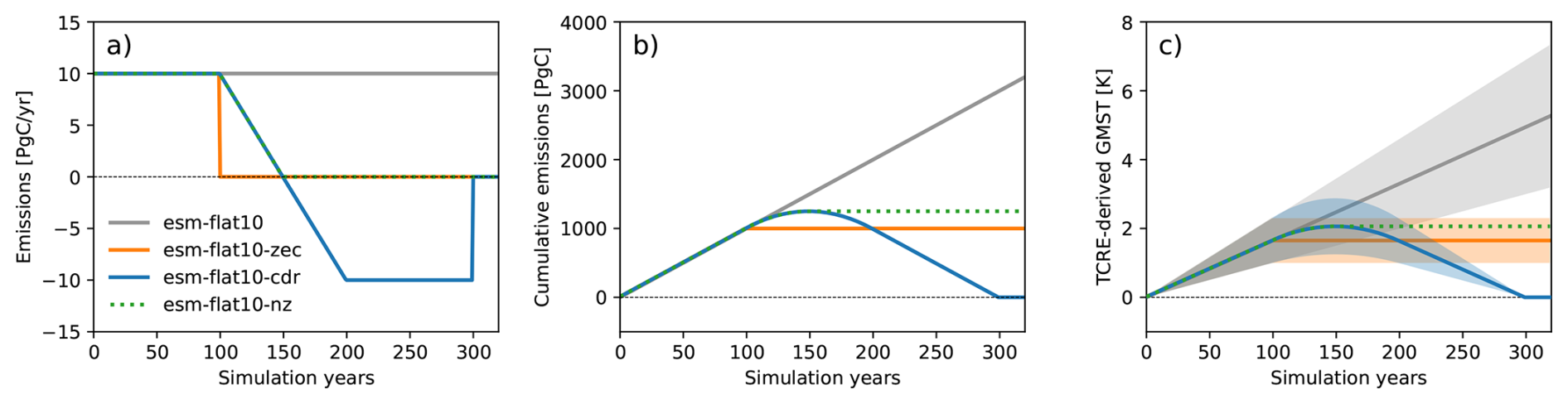
Figure 1 Experiment design. (a) and (b) show annual and cumulative carbon emissions as a function of time for the four experiments. (c) shows global mean surface temperature derived from cumulative emissions, assuming a perfectly linear TCRE relationship, with expected temperature evolution assuming cumulative emissions proportionality using the IPCC AR6 WGI best TCRE estimate (solid line, 1.65 °C per 1000 PgC) and likely range (shaded area, 1.0–2.3 °C per 1000 PgC) (IPCC, 2023b).

2.1 Experiments in flat10MIP

2.1.1 esm-flat10

The esm-flat10 experiment would serve as an emissions-driven experiment to diagnose the transient climate response to cumulative CO₂ emissions (TCRE), which is the warming from pre-industrial levels observed after the emission of 1000 PgC in a transient scenario. The esm-flat10 experiment would branch from a stable esm-piControl simulation, with a constant annual prescribed anthropogenic flux of carbon of 10 PgC yr⁻¹ into the atmosphere, with globally homogenous emissions. In esm-flat10, the 1000 PgC threshold would occur in year 100 – such that TCRE could be estimated as the time average between global mean warming in years 90–110, sampling over internal variability in this period. As such, we refer to TCRE derived from esm-flat10 and 1pctCO2 as T_100 yr and T_1000 PgC, respectively. The protocol for esm-flat10 is to continue emissions at 10 PgC yr⁻¹ for the duration of the experiment. In this ensemble, 150 years were considered to allow the simulation to reach 2× pre-industrial CO₂ concentrations in most cases (allowing for a wide range of plausible land and ocean carbon uptake). However, for future experiments in CMIP7 and beyond, a 300-year or longer esm-flat10 would be useful to explore potential nonlinearities in response to higher cumulative emission levels, which have been observed in some models (Schwinger et al., 2022).

2.1.2 esm-flat10-zec

The esm-flat10-zec experiment serves as an emissions-driven experiment to diagnose ZEC, which is the additional warming seen a certain number of years after the abrupt cessation of emissions. The esm-flat10-zec experiment would branch from year 100 of the esm-flat10 experiment, with an immediate cessation of emissions, and the system is then left to evolve for 220 years.  ZEC50 is calculated as the average temperature change relative to that when emissions cease, averaged over a 21-year period, 50 years after the cessation of emissions (i.e., years 140–160). ZEC90 is similarly calculated using years 180–200. For CMIP7 and beyond, we recommend 300 years for esm-flat10-zec to allow for longer timescale comparisons with esm-flat10-cdr.

2.1.3 esm-flat10-cdr

The esm-flat10-cdr experiment serves as an emissions-driven experiment to diagnose the response of the climate system to reducing, and ultimately reaching, net-negative emissions and will provide a measure of climate reversibility when all cumulative anthropogenic emissions are removed (i.e., all cumulative emissions and removals sum to zero) at the end of the experiment. The esm-flat10-cdr experiment would branch from year 100 of the esm-flat10 experiment, with a linear ramp down of emissions (from a starting point of 10 PgC yr⁻¹) of −0.2 PgC yr⁻¹ – such that net-zero emissions are achieved in year 150 and a negative flux of −10 PgC yr⁻¹ is achieved in year 200. This negative emission flux of −10 PgC yr⁻¹ would then be held constant from years 200–300, such that, by year 300, cumulative emissions from the start of the simulation would be zero. A 20-year extension follows, keeping the emissions at zero. For CMIP7 and beyond, we recommend 300 years for esm-flat10-cdr to allow for better evaluation of system dynamics after the termination of negative emissions.

2.1.4 esm-flat10-nz

We propose a final experiment for CMIP7 and beyond (not conducted here, but noted for its relevance), i.e., esm-flat10-nz (Sanderson et al., 2024), which branches from esm-flat10-cdr in year 150 at the point at which the simulation reaches net-zero CO₂ emissions, keeping emissions at zero thereafter. Such an experiment would provide a proxy for warming commitment after a gradual semi-idealized emission reduction to net zero and would provide additional information on ZEC. We recommend that such an experiment should run ideally for 250 years to allow for comparison of long-term dynamics with esm-flat10-zec and esm-flat10-cdr. Such an experiment could help differentiate the response of the system to negative emissions in esm-flat10-cdr from the delayed response to positive emissions and would provide a counterpoint to the abrupt emissions termination seen in esm-flat10-zec – providing an idealized scenario that might provide a more policy-relevant estimate of ZEC dynamics, reaching net zero after a period emissions reduction.

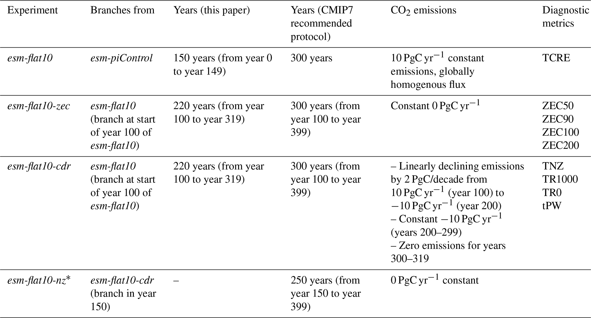
Table 1 Experiment design for emissions-driven diagnostic runs, detailing the branch point, length and configuration of the experiments as conducted in flat10MIP (present study). The CMIP7 recommended protocol includes run lengths and experiments suggested for future multi-model comparisons, including esm-flat10-nz, which is not conducted in this study.

The esm-flat10-cdr experiment allows for a number of simple idealized diagnostics that are relevant to the net-zero transition and the response of the system to net-negative emissions (Fig. 2). Like ZEC, each of these metrics is a measure of the path dependence of the temperature to the cumulative emissions relationship and thus would have a value of exactly 0 if global temperature response exactly followed TCRE proportionality. They include the following.

• Temperature difference at net zero (TNZ): this measures the error associated with assuming cumulative emissions proportionality to predict temperatures at net zero. esm-flat10-cdr reaches net-zero emissions in year 150, with cumulative emissions of 1250 PgC (calculated from year 1; see Fig. 1). TNZ is calculated as a 21-year average around year 150 in esm-flat10-cdr (i.e., 50 years after branching from esm-flat10) minus the expected temperature at net zero using cumulative emissions proportionality (T_ref, which is 1.25 times the esm-flat10-derived TCRE; see Fig. 2).

• Temperature asymmetry under CO₂ removal at 1000 PgC (TR1000): this measures the asymmetry in warming during positive and negative emissions at the same net cumulative emissions. It is calculated as a 21-year average around year 200 in esm-flat10-cdr minus a 21-year average around year 100 in esm-flat10. TR1000 would be a measure of hysteresis in global mean temperature when cumulative emissions return to 1000PgC on the downward branch minus the warming at the same cumulative emissions level under esm-flat10. This could be calculated using a combination of the esm-flat10 and esm-flat10-cdr experiments for a cumulative carbon emissions total of 1000 PgC.  esm-flat10-cdr reaches 1000 PgC cumulative emissions in year 200 on the downward branch (see Fig. 1). esm-flat10 itself reaches 1000 PgC in year 100.

• Temperature asymmetry under CO₂ removal at 0 PgC (TR0): this is a measure of carbon–climate reversibility when all previously-emitted carbon has been removed from the atmosphere. It is calculated as the average of years 301–320 in esm-flat10-cdr minus mean global temperatures in esm-piControl. TR0 is a measure of hysteresis in the global mean temperature when cumulative emissions return to zero after a period of negative emissions. This is calculated using a combination of the esm-piControl and esm-flat10-cdr experiments. esm-flat10-cdr reaches zero cumulative emissions in year 300 on the downward branch (see Fig. 1).

• Time to peak warming (tPW): this is a measure of the difference in timing between net zero and peak warming. It is calculated as the time difference between the peak value of 20-year smoothed global mean temperatures and the point that net zero is achieved in esm-flat10-cdr (year 150). This metric has a clear policy-relevant translation as the expected time it will take for the climate system to achieve maximum CO₂-driven global warming after (or before) reaching net-zero emissions under a smooth positive-to-negative emissions transition.

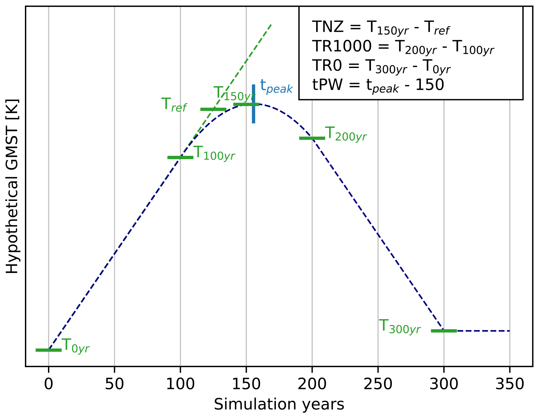
Figure 2 Schematic of metrics derived from the esm-flat10-cdr experiment to quantify different aspects of temperature reversibility under a continuous transition from positive to negative emissions. Dashed lines correspond to temperature trajectories for a hypothetical case where temperatures do not perfectly follow cumulative CO₂ emissions. GMST denotes global mean surface temperature.

2.2 Models used in flat10MIP

This ensemble provides a broad range of climate model structures and components to evaluate emissions-driven climate reversibility. We include eight CMIP6 generation Earth system models (ESMs), one CMIP3 generation model, one intermediate complexity model and the three simple climate model (SCM) ensembles used in the AR6 IPCC assessment (Forster et al., 2023). The ESMs and SCMs participating in this study are listed in Table 2 and more fully described in the Appendix. Each Earth system model has completed one ensemble member of each of the MIP experiments (esm-flat10, esm-flat10-cdr and esm-flat10-zec) – with supporting existing experiments from CMIP6 (C4MIP, ZECMIP and CDRMIP). We note that metrics from Earth system models, unlike SCMs, are subject to uncertainty arising from internal variability. We would encourage centers to perform at least three members of these experiments in CMIP7 to provide better sampling and estimation of the role of initial condition uncertainty. For each SCM, approximately 1000 simulations are completed with simple climate model versions spanning a range of climate responses consistent with assessed climate uncertainty (using a combination of observational constraints, IPCC-assessed ranges and ESM data to constrain the parameter space of the simple climate models (IPCC, 2023d)).

In this study, we summarize the global mean characteristics of the simulations used to conduct the experiments, while additional dedicated domain-specific studies will assess regional aspects of transient-emissions-driven response and reversibility.

3 Results

Figure 3 illustrates the global temperature response for the three simulations requested in flat10MIP. Throughout this section, we refer by default to T_100 yr – the warming, in units K, after 1000 PgC of cumulative emissions (which in esm-flat10 occurs in year 100). T_100 yr is numerically equivalent to TCRE (units K/1000 PgC) but allows proper consideration of the arithmetic sum with ZECn, also in units K. Summary metrics, as defined above for each model, are detailed in Table 2. Figure 3a shows that the range of T_100 yr seen in the ESM ensembles (1.1–2.4 K) is broadly captured by the SCM ensembles considered in this study, though MAGICC shows a greater upper bound in T_100 yr (10th–90th percentile of 1.1–2.7 K) relative to FaIR or CICERO-SCM (10th–90th percentiles of 1.1–2.1 and 1.2–2.1 K, respectively). However, we see differences in the ZEC50, ZEC90 and reversibility distributions. The ESM ZEC90 distribution is best captured by FaIR (ZEC90 range of −0.1 to +0.2 K), whereas MAGICC and CICERO-SCM simulate more negative values (−0.2 to +0.1 K and −0.3 to −0.1 K, respectively). We also see that two of the three SCM ensembles (MAGICC and CICERO-SCM) tend to simulate a stronger temperature decline under negative emissions than seen in any of the ESMs, although the FaIR ensemble is broadly consistent. The intermediate complexity model, UVic-ESM, lies within the ESM distribution for both T_100 yr and ZEC90.

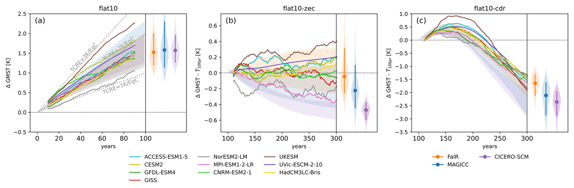
Figure 3 Summary results for global mean surface temperature (GMST) response in the trial flat10MIP. Colored lines indicate temperature change from (a) pre-industrial levels to (b, c) T100 yr (the average temperature in years 91–110 in esm-flat10) in each of the participating ESMs. Shaded regions refer to the simple climate models' probabilistic distribution ranging from the 10th to 90th percentiles. This distribution is shown as violin plots for the last time step of each scenario, where the shading shows the full range of results and the vertical line indicates the 10th–90th percentiles, with the median in the center. A 20-year moving average is applied to all time series.

3.1 Earth system model responses

Figure 4 illustrates the ESM results in more detail, showing the evolution of a number of climate indicators. In esm-flat10, emissions are constant at 10 PgC yr⁻¹ – and thus temperature change from pre-industrial to year 100 is a measure of the transient response to cumulative CO₂ emissions. Figure 4a illustrates the range of transient response in the context of the assessed TCRE range in IPCC AR6 (1.0 to 2.3 K (1000 PgC)⁻¹) (IPCC, 2023a). The models considered in the present MIP largely span this range, with values of TCRE (as calculated from 1pctCO2) from 1.2 to 2.6 K (Table 2). The model land sink evolution varies during the extended esm-flat10 simulations, with some models showing a saturation of the land sink (HadCM3, UVic, ACCESS) and others showing continued land uptake throughout the experiment (CESM, NorESM, GFDL, CNRM).

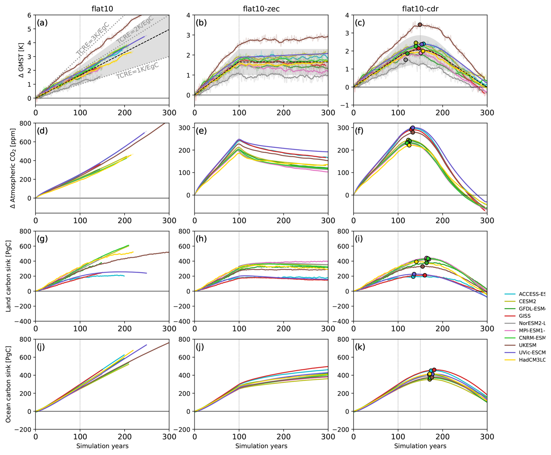
Figure 4 ESM results. Columns represent global indicators from ESM simulations running esm-flat10 (left), esm-flat10-zec (center) and esm-flat10-cdr (right). Panels (a)–(c) show changes in GMST, with the black dashed line and gray shading denoting the central estimate and range derived from cumulative emissions, assuming a linear TCRE relationship as given in AR6 (TCRE = 1.65 K, likely range of 1.0–2.3 K) for reference. Panels (d)–(f) illustrate changes in atmospheric CO₂ concentrations as a function of time. Panels (g)–(i) show cumulative carbon absorption by the land surface. Panels (j)–(l) show cumulative absorption of carbon by the ocean over time. The circles for the esm-flat10-cdr experiments indicate the maximum of each time series. A 20-year moving average is applied for the GMST time series (bold line); the faint line shows the original data.

Figure 4b shows how temperatures evolve in esm-flat10-zec – showing that temperatures remain (approximately) stable following the cessation of emissions, even though atmospheric carbon dioxide concentrations decline. Different models show a diversity of evolution of land and ocean carbon sinks – with some models (e.g., MPI, GFDL, GISS) initially absorbing land carbon for the first 20–50 years of the zero-emissions phase before losing carbon on longer timescales, while the land sink in other models (UVic, GISS, HadCM3, UKESM) stabilize the land sink after emissions cessation. Ocean uptake is more consistent across the ensemble, with all models simulating a continued uptake of carbon in the ocean during the zero-emissions phase.

The global mean results for esm-flat10-cdr are summarized in Fig. 4c, showing that peak warming can occur either before or after net zero (but most models peak before), as seen in similar experiments (Koven et al., 2023) and ZECMIP experiments (Jenkins et al., 2022). By the end of the simulation, some models remain warmer than the pre-industrial period (CESM, CNRM, ACCESS, UVic), while some are cooler (GISS, MPI, NorESM, GFDL). All models are in agreement that peak CO₂ concentrations occur before net zero, and all models predict that the ocean carbon sink peaks after net zero. All models predict that the cumulative ocean carbon sink will decline but stay positive. However, models disagree on the timing of the peak land sink relative to net zero. GFDL, CESM, NorESM, GISS, MPI and CNRM show the cumulative land carbon sink peaking after net zero, whereas HadCM3, UVic and ACCESS show the cumulative land carbon sink peaking before net zero. At zero cumulative emissions in year 300, models range from the cumulative land sink being near-zero to being a slight net source of carbon over the 300-year period (model range: −50 to 0 PgC), while all models agree that the cumulative ocean sink is a net sink (model range: 120–220 PgC).

Figure 5 shows how the rate of carbon emission allocation to the atmosphere, land and ocean evolves as a function of time in the different experiments. In esm-flat10, we observe a transition from an initially high airborne fraction towards increasing allocation to land and ocean pools, with the airborne fraction in year 100 ranging between 0.45 and 0.55 across models. This variation arises from inter-model differences in the representation of land and ocean carbon uptake processes. For example, some models exhibit sustained terrestrial uptake (e.g., CESM2, NorESM2), while others (e.g., ACCESS, UKESM) show land sink saturation or reversal, likely reflecting the interplay between CO₂ fertilization (Arora et al., 2020), nutrient availability (Goll et al., 2012) and warming-induced soil carbon losses (MacDougall et al., 2020; Wieder et al., 2013). Declining land uptake in some models may also reflect increasing hydrological stress or climatic constraints on productivity (Fisher et al., 2019). During the esm-flat10-zec experiment, atmospheric CO₂ declines following cessation of emissions, but models diverge in whether this drawdown is primarily balanced by land (e.g., GFDL, CNRM) or ocean (e.g., GISS, ACCESS) uptake. These differences reflect the distinct timescales and sensitivities of the carbon pools: the land sink responds quickly to emissions cessation but may decay as CO₂ fertilization effects diminish and heterotrophic respiration increases (Jones et al., 2013), while the ocean continues to absorb carbon due to its longer equilibration timescales and sustained pCO2 disequilibrium (Schwinger and Tjiputra, 2018; Tjiputra et al., 2013) and the model-specific representation of deep ocean ventilation and carbon transport (Séférian et al., 2024). The resulting diversity in sink partitioning highlights key model-dependent feedbacks in the terrestrial biosphere and ocean circulation, which modulate the climate system's reversibility following net zero.

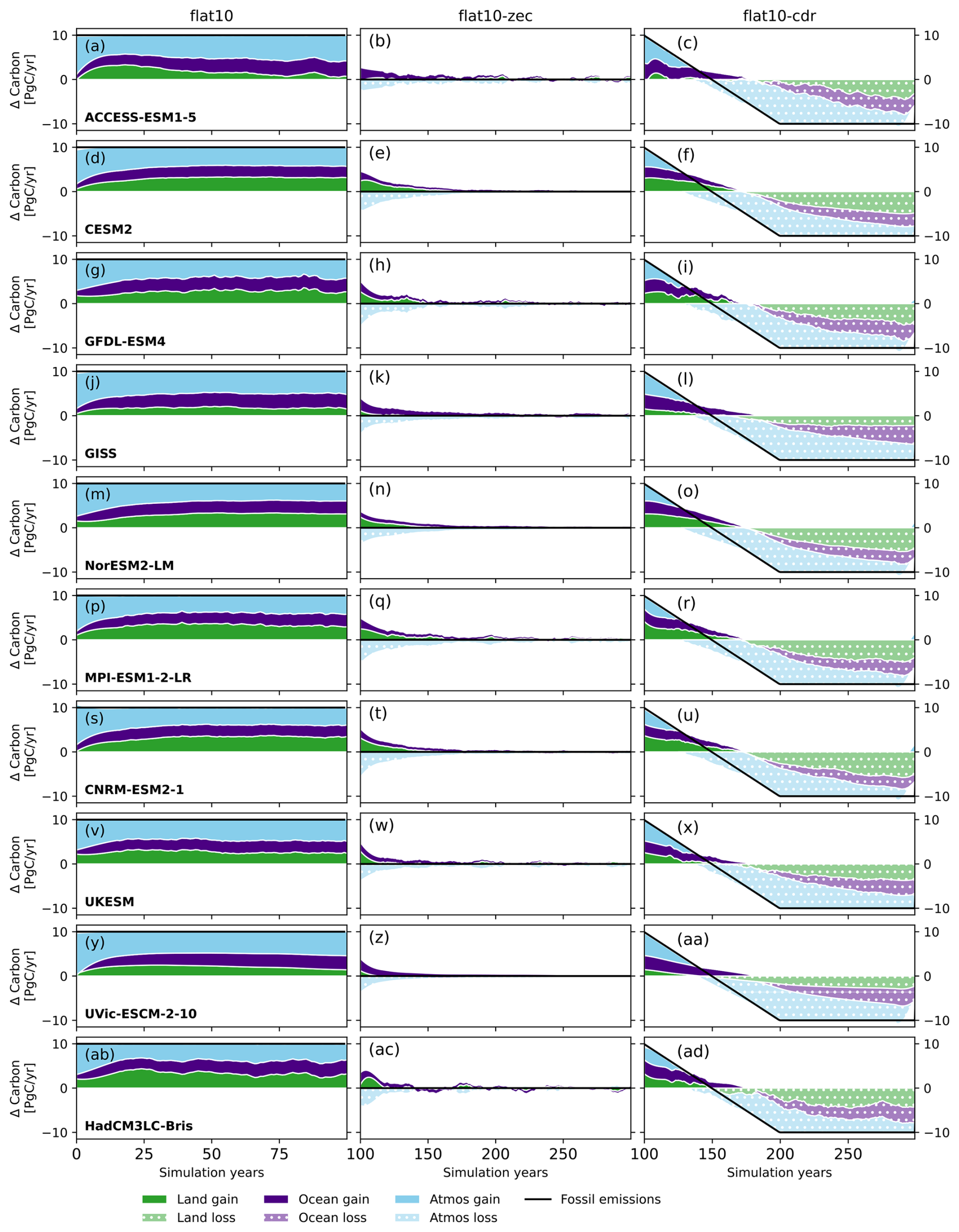
Figure 5 Evolution of carbon sinks in ESMs in flat10MIP. [Light blue/dark blue/green] shading shows the [airborne fraction/ocean fraction/land fraction] of emissions in each year as a function of time. Gains for each domain are shown in solid colors, while losses are shown in light dotted colors. The left-hand column shows the fractions for esm-flat10, where emissions total 10 PgC yr⁻¹. The central column shows results for esm-flat10-zec, where emissions are zero and atmospheric loss is compensated by gains in the land and ocean. The right-hand column shows esm-flat10-cdr, where removals are balanced by losses from each of the pools.

3.2 Global response indicators in flat10 and other experiments

3.2.1 Transient climate response to positive emissions

Figure 6 and Table 2 illustrate the global trajectories and summary indicators of the ESMs that participated in the experiment set in both esm-flat10 and 1pctCO2 (drawing on results from Arora et al., 2020). Figure 6a shows that this compatible emissions time series is time-varying and model-dependent – with typical behavior showing compatible emissions growing from ∼ 10 PgC yr⁻¹ at the start of the experiment to between 16 and 22 PgC yr⁻¹ at the time at which cumulative emissions reach 1000 PgC. As such, compatible cumulative emissions are weighted towards the end of the experiment – the mean result exceeds 500 PgC in year 39 and 1000 PgC in year 65 (Fig. 6b). Compatible emissions in 1pctCO2 are also significantly greater than current anthropogenic emissions (11.1 ± 0.8 PgC yr⁻¹ in 2023) (Friedlingstein et al., 2023).

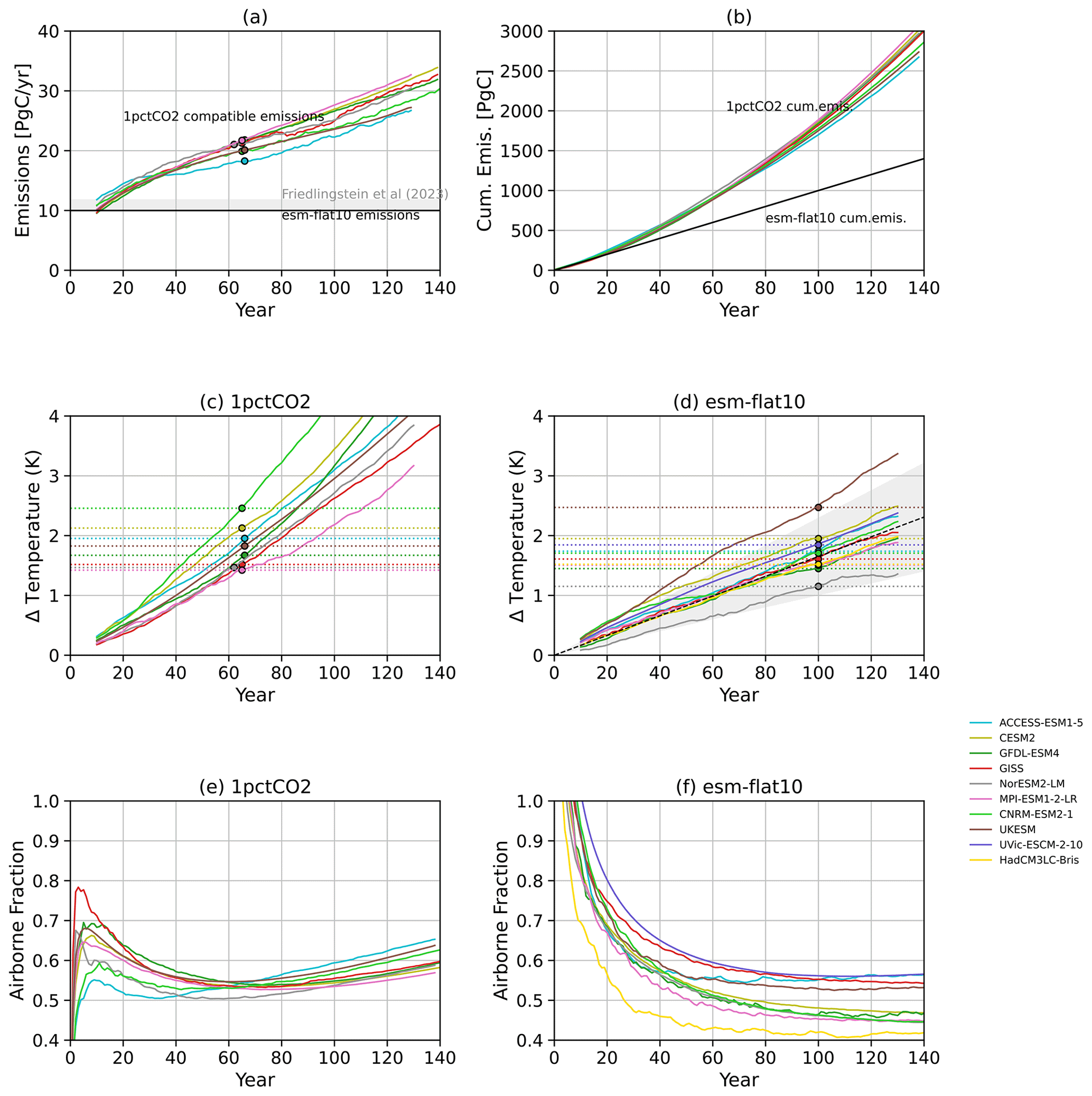
Figure 6 Comparative ESM results for TCRE calculation using 1pctCO2 and esm-flat10, showing (a), (b) compatible [annual, cumulative] emissions in 1pctCO2 compared with the constant 10 PgC yr⁻¹ flux in esm-flat10. Annual total anthropogenic carbon emissions in 2023 are shown for context. (c, d) show temperature evolution in [1pctCO2, esm-flat10]. Colored lines show global model output from available ESMs with a 21-year moving average applied. (e, f) show airborne fraction in [1pctCO2, esm-flat10]. Circles show results at the time when cumulative emissions reach 1000 PgC. Shaded region in (d) illustrates the range of warming according to the IPCC AR6-assessed likely range of TCRE.

Table 2 Summary diagnostics from flat10MIP and ZECMIP/1pctCO2 (MacDougall et al., 2020) experiments for Earth system models and simple climate models, which reported T_1000 PgC, ZEC50 and ZEC90. T_100 yr is the mean warming in years 91–110 in esm-flat10, and ZEC50/90/100 is the zero emissions commitment, measured as the warming in esm-flat10-zec between years 100 and years 150/190/200, respectively. t−PW is the time difference in years of peak warming in esm-flat10-cdr relative to net zero in year 150, and (TNZ/TR1000/TR0) is the warming in years (150/200/310) in esm-flat10-cdr relative to warming in years (125/100/0) in esm-flat10 when cumulative emissions are (1250 GtC/1000 GtC/0 GtC), respectively.

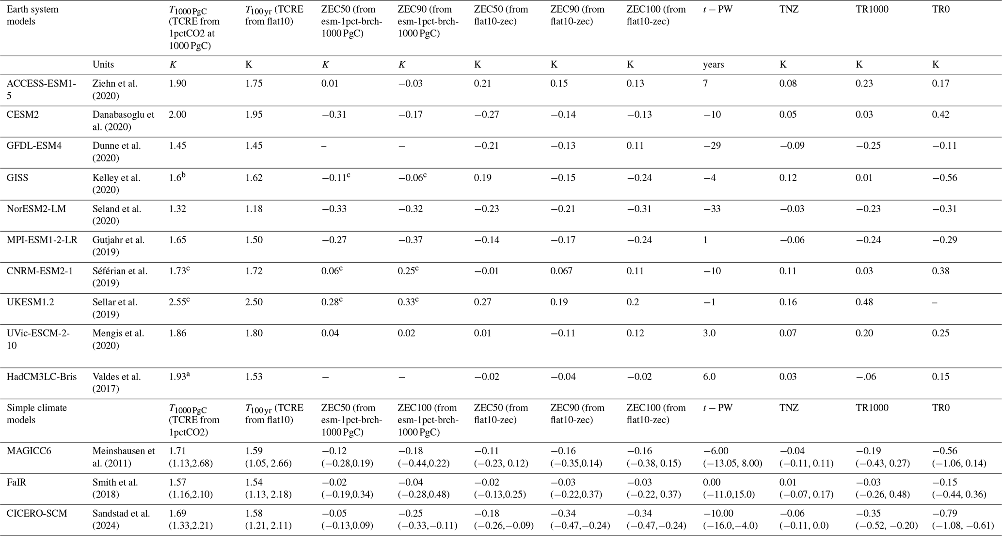
^a Chris Jones (personal communication, 2024). ^b Anastasia Romanou (personal communication, 2024). ^c 1pctCO2 responses are from a similar but non-identical previous model version.

Figure 7 compares distributions of T_100 yr and ZEC computed using the 1pctCO2 and esm-flat10 approaches. We see, on average, a slight offset such that TCRE estimates in the ESMs have a value that is an average of 0.12 K greater in 1pctCO2 relative to esm-flat10 (see Table 1, Fig. 7). This is consistent with Krasting et al. (2014), who found that TCRE estimated at high emissions rates was greater than that estimated using present-day emissions rates and attributed the difference to a greater disequilibrium between land/atmosphere and ocean response states when emissions rates are very high. Similarly, distributions in the simple climate models MAGICC and CICERO-SCM show that T_1000 PgC from 1pctCO2 is on average about 0.1 K greater than T_100 yr from esm-flat10. The third simple climate model, FaIR, shows comparable values of T_1000 PgC and T_100 yr (Fig. 7). Given that probabilistic calibration is performed independently for each SCM, it is not easy to attribute these differences to structural differences between the models or to choices of probabilistic parameter calibration strategy. Figure 8a shows correlations between T_1000 PgC and T_100 yr – re-enforcing the small average offset between the two approaches - though the gradient of the best fit line is near-unity.

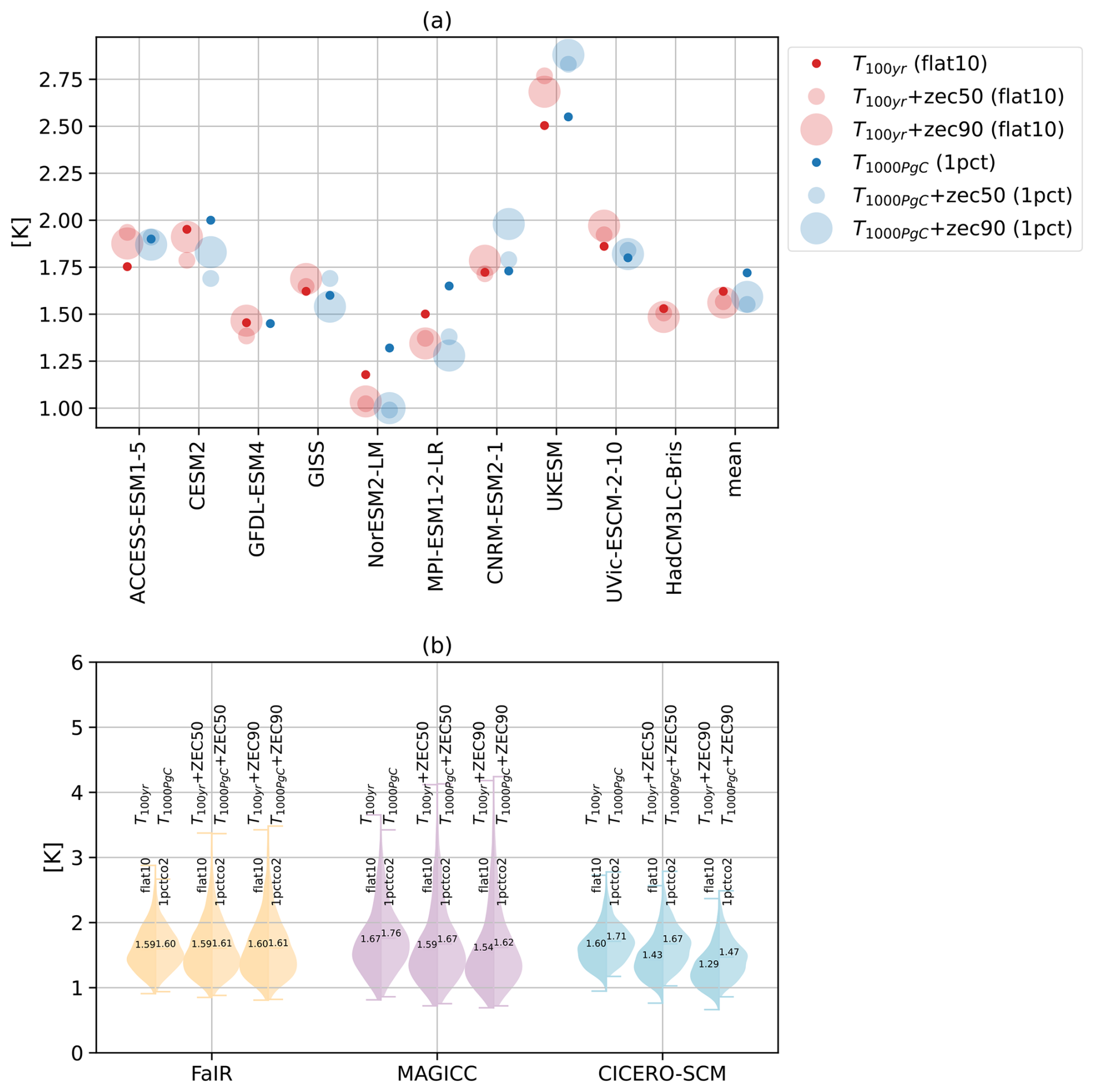
Figure 7 (a) A comparison of T_100 yr [flat10] and T_1000 PgC [1pctCO2], T_100 yr+ ZEC50 [flat10-zec]/T_1000 PgC+ ZEC50 [1pctCO2] (small transparent points) and T_100 yr+Z EC90 [flat10-zec]/T_1000 PgC+ ZEC90 [1pctCO2] (large transparent points) for ESMs participating in flat10MIP (red) and ZECMIP (blue, where available). The final point is the multi-model mean for cases where there exist complete runs for both ZECMIP and flat10MIP [ACCESS, CESM2, NorESM, MPI-ESM and CNRM-ESM2]. (b) For SCMs, violin plots showing distributions of T_100 yr, T_100 yr+ ZEC50 and T_100 yr+ ZEC90 for esm-flat10 (left) and 1pctCO2 (right).

3.2.2 Zero Emissions Commitment

For ZEC, however, we see greater differences between the concentration-driven approach and the emissions-driven approach than for TCRE (Figs. 7, 8, 9). In the SCM ensembles, ZEC50 and ZEC90 are on the order of 25 % smaller if measured using the flat10-zec protocol relative to the ZECMIP protocol (this is true irrespective of whether ZEC is positive or negative, Fig. 8c, d). This is consistent with MacDougall et al. (2020), who found smaller ZEC in experiments with lower emission rates up to the point of net zero, proposing that both warming and carbon cycle responses are closer to equilibrium. We also note that one SCM, CICERO-SCM, shows more consistently negative values of both ZEC50 and ZEC90 when quantified via flat10MIP than by ZECMIP (Fig. 8c, d). ESMs are also consistent with the relationship of ∼ 25 % smaller absolute magnitudes in ZEC50 and ZEC90, albeit with larger scatter. Some models (NorESM, CESM2, MPI, CNRM) in the ZECMIP experiment suggest an apparent short-term warming pulse following the cessation of emissions, which is less pronounced in the esm-flat10-zec experiment (Fig. 9) – but additional ensemble members are required to properly quantify this behavior. In the MPI model, this is consistent with findings that TCRE was higher using the ZECMIP protocol compared to flat10MIP (Fig. 1d in Winkler et al., 2024).

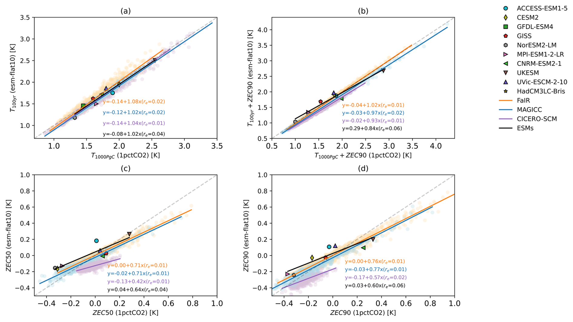
Figure 8 Comparison metrics assessed using the flat10MIP methodology and 1pctCO2-based experiments. ESM summary metrics are T_100 yr, ZEC50 and ZEC90 for esm-flat10 and T_1000 PgC and ZEC50 and ZEC90 for 1pctCO2. Filled shapes illustrate values assessed from ESMs, and pale dots illustrate members of the simple climate model ensembles for (FaIR, MAGICC, CICERO-SCM) in (orange, blue, purple). Straight lines show the least-squares best fits for the ESMs (black) and SCMs.

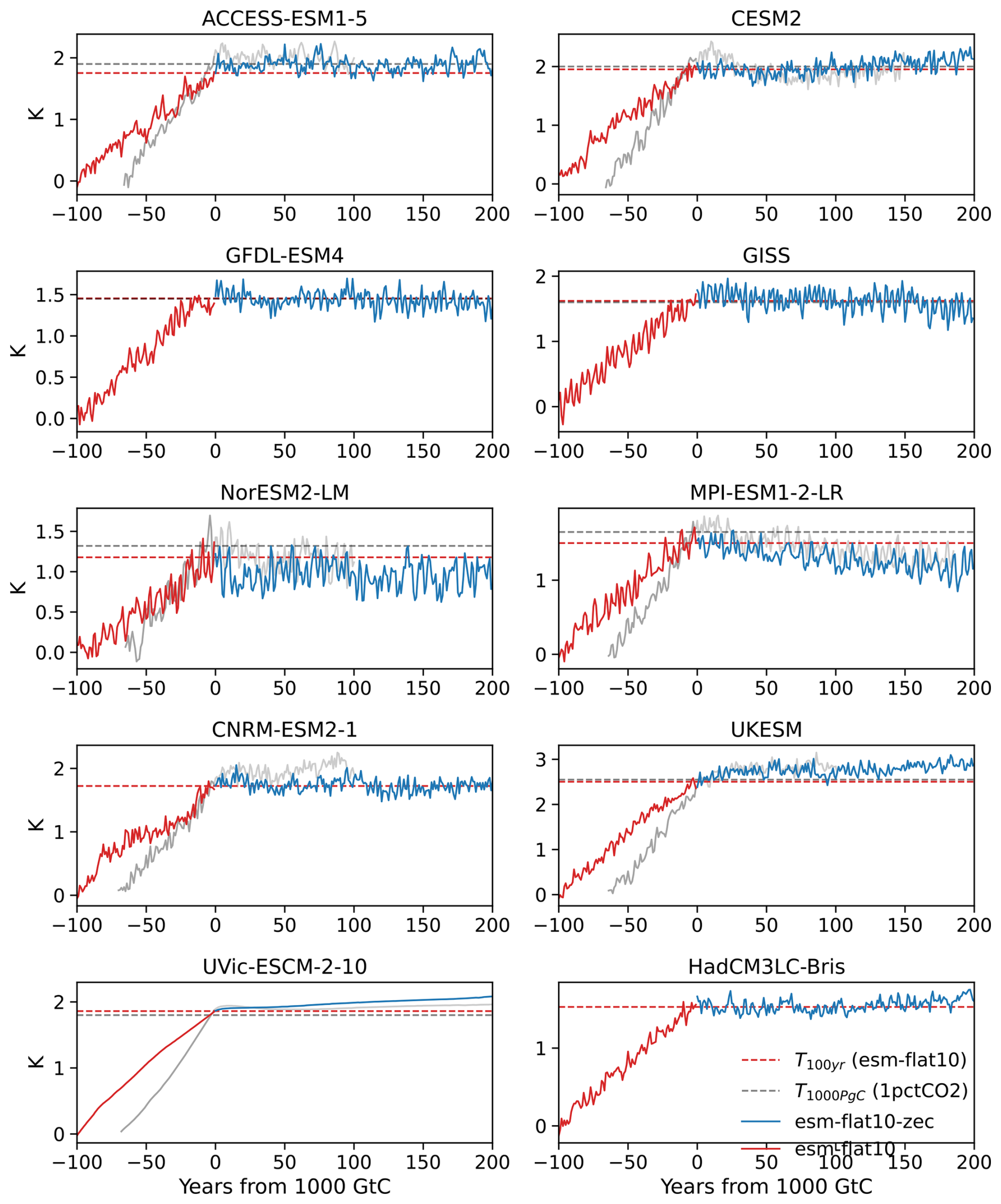
Figure 9 Global mean temperature change evolution for ESMs participating in flat10MIP (bold colors), in the context of 1pctCO2 (gray) and ZECMIP, where comparable simulations with the same model version are available (faded colors). Red lines show the positive emissions period (10 PgC yr⁻¹ for flat10 (solid red) and 1pctCO2-compatible emissions for ZECMIP), and blue/gray lines show the zero-emissions period for esm-flat10-zec and esm-1pct-brch-1000PgC, respectively. Horizontal dashed lines show [T_100 yr,T_1000 PgC] as estimated from [esm-flat10 (red), 1pctCO2 (gray)].

It is also evident that total warming measured from pre-industrial levels 100 years after emissions cease (i.e., T_100 yr+ ZEC90 from esm-flat10 and T_1000 PgC+ ZEC90 from 1pctCO2) is more consistent between the ZECMIP and flat10MIP protocols (Fig. 8b) than either TCRE or ZEC90 independently – indicating that total warming following a period of emissions followed by cessation is path-independent in the models considered here. However, we continue to see in the mean values of the SCM distributions (Fig. 7b) for MAGICC and CICERO-SCM that T_1000 PgC+ ZEC90 is ∼ 0.1 K greater in esm-flat10-zec than in esm-1pct-brch-1000PgC. FaIR is again consistent between the two approaches, with only a 0.01 K difference between the mean values. For the ESMs (Fig. 7a), we note that the multi-model mean T_1000 PgC+ ZEC90 is 0.05 K greater for esm-1pct-brch-1000PgC than T_100 yr+ ZEC90 for esm-flat10-zec (whereas the mean T_1000 PgC is 0.12 K greater than T_100 yr).

Our results in general suggest that the weighting of compatible emissions towards the end of the simulation in 1pctCO2, as well as the shorter total time period over which emissions occur in 1pctCO2 (∼ 70 vs 100 years), has an impact on both the estimate of TCRE and the transient response following cessation of emissions. We tend to see slightly greater estimated values of TCRE in 1pctCO2, with most models exhibiting short-term continued warming followed by cooling in the decades following cessation of emissions. In contrast, the behavior in esm-flat10-zec exhibits slightly less warming during the positive emissions phase and less adjustment afterwards, resulting in lower values for TCRE and smaller magnitudes (either positive or negative) of ZEC50 and ZEC90. The finding that ZEC50/90 from esm-flat10 is lower than ZECMIP estimates is consistent with the findings of Jenkins et al. (2022), who found that ZEC is modulated by “average cumulative emissions over the period”, a metric that is different under the two experimental designs.

3.2.3 Climate reversibility experiments

The global mean results for esm-flat10-cdr are shown in Fig. 4. The temperature response at year 300 (when cumulative emissions return to zero) shows a range of −0.7 to +0.5 K, indicating notable deviations from cumulative emissions proportionality with residual warming or cooling depending on the model. Figure 10 illustrates global-scale hysteresis in the ESM results, showing the change in global mean surface temperature as a function of cumulative emissions. Though all models broadly indicate proportionality between temperature and cumulative emissions, there are some notable deviations. Many models indicate some hysteresis, either positive (ACCESS) or negative (GFDL, NorESM, MPI-ESM), between the upward and downward branches of the simulation, and some (CESM2, GFDL, CNRM) appear to show a change in temperature/cumulative emissions response during the course of the downward branch. Overlain as dotted lines on each panel of Fig. 10 is a null hypothesis, informed only by TCRE and ZEC90 from the esm-flat10 and esm-flat10-zec experiments, that temperatures in the net-negative emissions period of esm-flat10-cdr might be explained as a combination of the TCRE ⋅ I_em+ ZEC terms (Koven et al., 2022, 2023). This framework explains some, but not all, of the hysteresis observed; in particular, some of the models (e.g., GFDL, UKESM) show a larger hysteresis than predicted by ZEC90, and the TCRE + ZEC framework does not predict the deviations late in the downward branch for those models that have such dynamics. Alternative frameworks such as RAZE (Jenkins et al., 2022) explain other key features – such as the expectation in a symmetrical experiment such as esm-flat10-cdr that half of the ZEC is manifested at the time of net zero. A unifying explanation for these frameworks that is accurate both during the net-zero transition and at timescales significantly before and after remains absent from the literature to date.

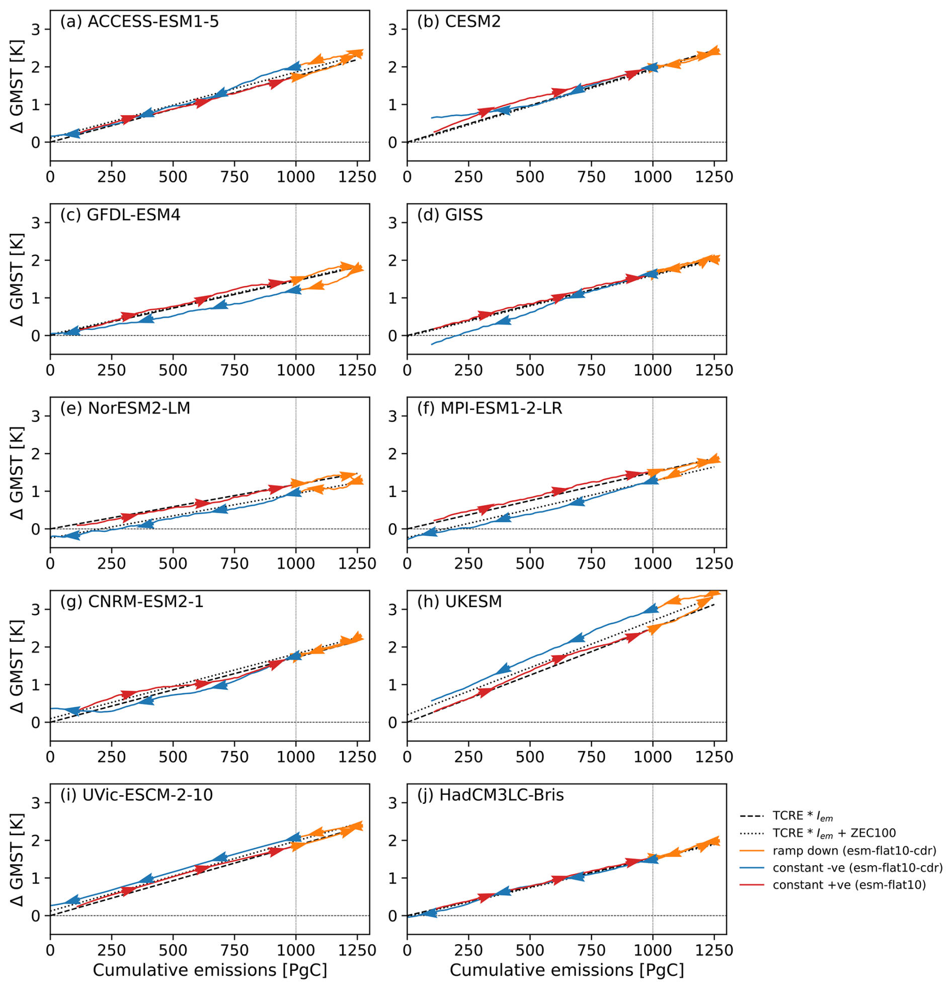
Figure 10 Global mean temperature relationship with cumulative emissions for the ESMs. A 21-year moving average is applied for the GMST time series. Arrows show the direction of time, with [red, yellow, blue] lines showing [constant positive, ramp down, constant negative] phases of the experiment. Black dashed and dotted lines show TCRE ⋅ cumulative emissions (I_em) and TCRE ⋅ cumulative emissions + ZEC90 for each model, using TCRE and ZEC90 values as calculated from esm-flat10 and esm-flat10-zec.

Figure 11 indicates the ESM ensemble distribution of temperature evolution in the esm-flat10-cdr, normalized by expected warming from TCRE. The figure shows that TCRE proportionality is consistent between models in the ensemble, with a relatively small spread during the constant positive emissions phase of the experiment. As the emissions rate reduces and becomes negative, additional spread but no systematic direction of asymmetry is seen relative to expectations from TCRE alone – and this spread remains constant throughout the negative emissions phase. We can categorize this uncertainty as approximately ±10 % of TCRE, which remains broadly constant over time during the negative phase.

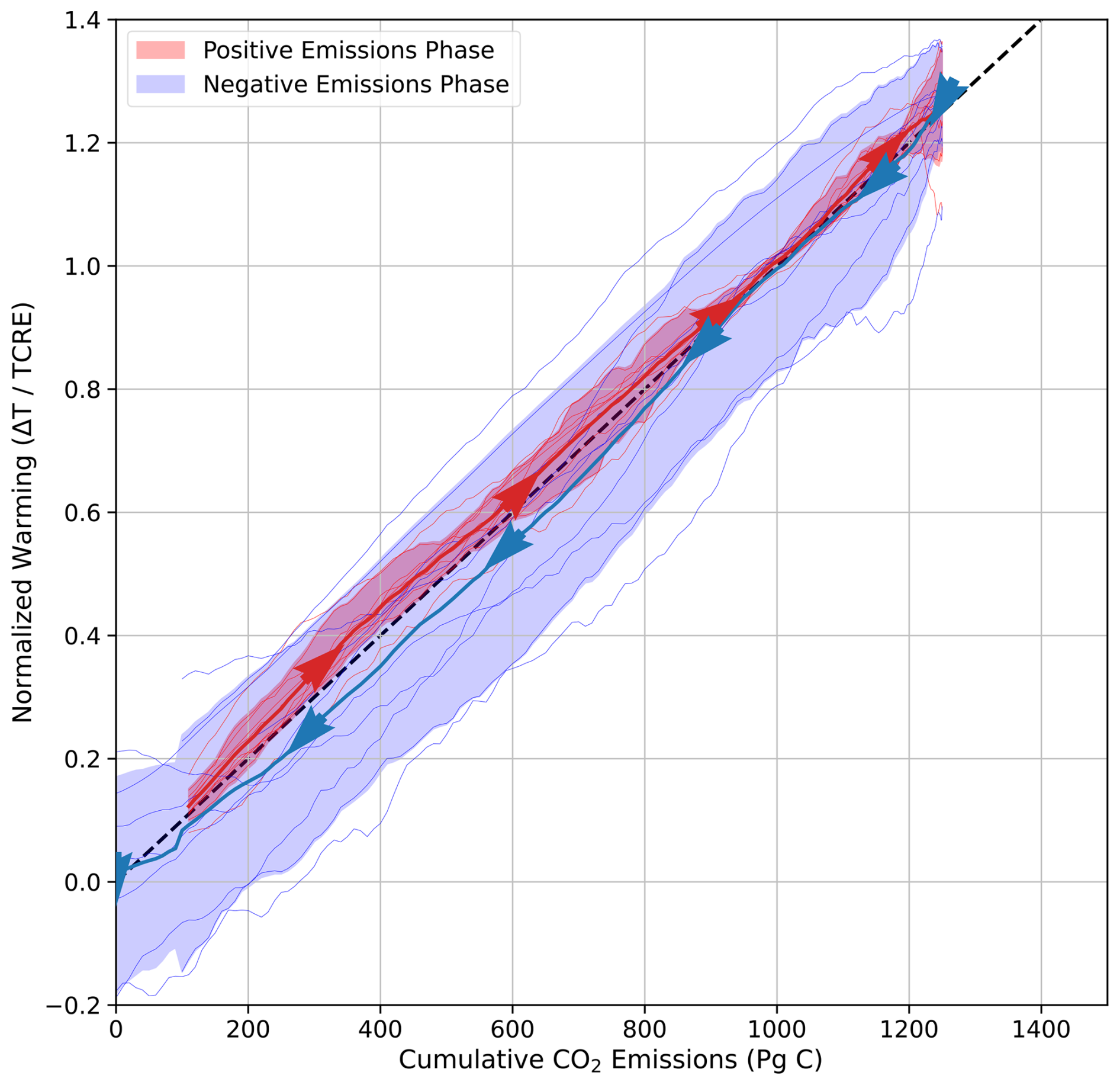
Figure 11 Global mean temperature relationship with cumulative emissions for the ESM distribution in esm-flat10-cdr, normalized by TCRE as estimated from esm-flat10. A 21-year moving average is applied for the GMST time series. Arrows show the direction of time, with [red, blue] lines showing multi-model mean [positive, negative] emissions phases of the experiment. [Red, blue] shaded regions indicate the [10th, 90th] percentiles of the ESM ensemble temperature distribution at a given cumulative emissions level. Black dashed line shows the normalized relationship between cumulative emissions and warming.

Figure 12 shows how additional climate indicators vary with cumulative emissions. Atmospheric carbon dioxide levels are consistently lower on the downward branch, but cumulative land carbon sink hysteresis varies by model – with some models showing significantly larger cumulative land carbon sinks on the downward branch (e.g NorESM), while other models (e.g., GISS, HadCM3LC) show cumulative sinks proportional to cumulative emissions on both the upward and downward branches. Similarly, all models show a hysteresis in cumulative ocean sink strength with cumulative emissions, with between 100 and 200 PgC remaining in the ocean in year 300 of esm-flat10-cdr.

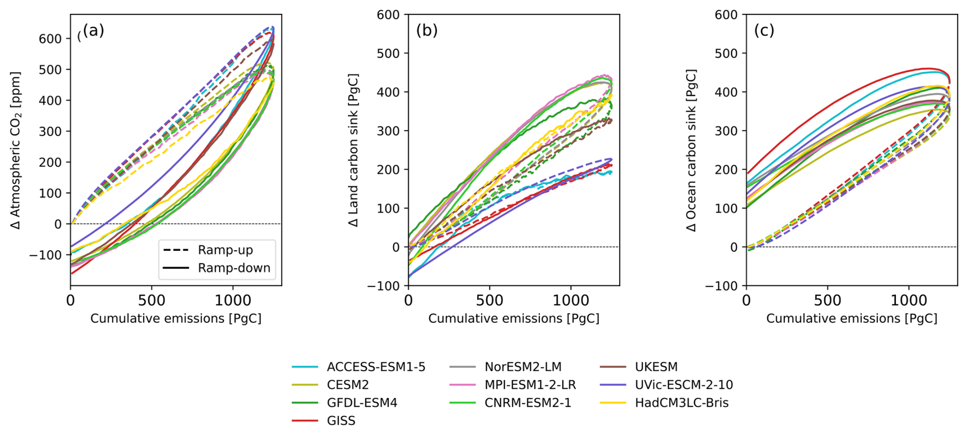
Figure 12 Climate indicators as a function of cumulative emissions for the ESMs. A 21-year moving average is applied for all time series.

We identify a number of new metrics  (TNZ, TR1000, TR0 and tPW; Fig. 2, Table 2), which are aimed at capturing aspects of climate reversibility and commitment from the flat10-cdr experiment. As noted above, each of these measures a distinct aspect of potential deviation from perfect TCRE proportionality and thus, like ZEC, would have a value of exactly 0 if temperatures were exactly proportional to the cumulative emissions.

Two of these metrics measure the hysteresis around the net-zero transition: tPW is the time offset of peak warming relative to net zero, whereas TNZ is the difference in realized temperature at net zero relative to what one would predict through TCRE proportionality. Figure 13 shows how these metrics relate to each other and to TCRE and ZEC. With the exception of TCRE, all metrics show a positive correlation with all other metrics, particularly for SCMs. ESMs show greater scatter across a number of the pairwise relationships than the SCMs, reflecting a greater diversity of potential dynamics arising from their high complexity than are being captured in the more parsimonious relationships represented by the SCMs. For example, in each of the SCM ensembles, tPW and TNZ are highly and consistently related, but a number of ESMs (CNRM, GISS, CESM, UKESM) lie outside of the SCM distributions such that we see peak warming significantly before net zero with greater warming than one would expect from cumulative emissions proportionality (contours in Fig. 13 indicate 90 % of the ensemble distribution; for tPW vs TNZ, the ESM results lie outside of the 99th percentile (not shown)). Similar differences are seen in the relationship between tPW and ZEC50, with two ESMs showing peak warming occurring particularly early. This hints at behavior in the ESMs that might not be represented in the current generation of SCM parameter ensembles. This could potentially be due to an absence of ZEC or reversibility-related metrics used in the calibration pipelines. Alternatively, this could potentially be due to a number of different processes, e.g., ocean circulation processes such as AMOC weakening, which are not represented in current SCMs (Schwinger et al., 2022), but larger ESM initial condition ensembles are necessary to have confidence in the ESM metrics in the presence of internal variability.  This discrepancy could potentially be related to studies that have found inconsistencies between the temporal dynamics of the ocean heat and carbon uptake in ESM and SCM ensembles (Séférian et al., 2024) and would benefit from further investigation.

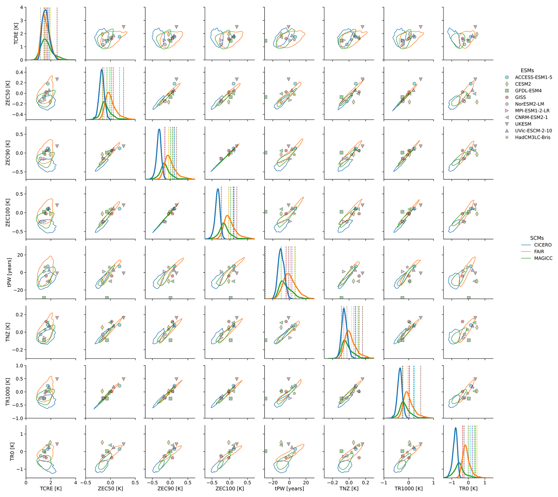
Figure 13 Matrix of relationships between metrics quantified here. Shown are pairwise plots between the following metrics: TCRE (T100yr for flat10 and T1000PgC for 1pctCO2), ZEC50, ZEC90, ZEC100, tPW, TNZ, TR1000 and TR0. SCM ensembles are shown as contours at the 10th percentile of the joint distribution for each pairwise comparison (such that 90 % of points lie within the contours, with FaIR, MAGICC and CICERO-SCM in orange, green and blue, respectively). ESMs are shown as individual points. Diagonal panels show histograms (SCMs) and discrete values (ESMs) for each of the metrics diagnosed here.

Another pattern that emerges in Fig. 13 is the greater correlation captured in the short-term metrics (ZEC50, TR1000) than in the longest-term metric (TR0) that shows greater scatter with the ZEC and other reversibility metrics. This high correlation (e.g., between ZEC50 and TR1000 and between ZEC100 and TR1000) has an important implication: most of the uncertainty present in the reversibility of GMST (although not necessarily regionally or in other metrics; Schleussner et al., 2024) under an idealized overshoot scenario will also be present under zero emissions at the same level of cumulative emissions that avoids the overshoot.

4 Summary and conclusions

The finding of a near-linear relationship between cumulative carbon emissions and global mean temperature (Allen et al., 2009; Matthews et al., 2009) enabled recent climate policy to link desired limits for warming to an allowable budget of remaining carbon emissions. The years following have seen regular efforts to quantify remaining carbon budgets for the Paris Agreement goals (Lamboll et al., 2023), with scenarios built on this premise (Rogelj et al., 2019a), and refinement in the treatment of how to incorporate non-CO₂ emissions into this framework (Cain et al., 2019; Jenkins et al., 2018; Mengis and Matthews, 2020).

Further, an increased understanding has emerged that the TCRE relationship is an approximation, owing to fortuitous cancellation of terms in heat and carbon uptake in many models, but this cancellation is not perfect, and a Zero Emissions Commitment (ZEC; Palazzo Corner et al., 2023) may result in residual carbon-induced warming (or cooling) even if carbon emissions are held at net zero. This ZEC effect may cause peak temperatures to be seen before or after net zero (Koven et al., 2023). Building confidence in this timing is important; if peak temperatures occur after net zero, this may create climate adaptation challenges that might not otherwise be planned for if simple TCRE proportionality is used to predict warming outcomes.

Operational methods of quantifying TCRE and ZEC to date have utilized existing default Earth system model diagnostic experiments that have focused on the response of the Earth system to a prescribed concentration pathway – generally an exponential increase of 1 % per year – as an idealized proxy for climate change induced by carbon dioxide. It is then possible to calculate compatible CO₂ emissions, specific to a given model, to frame the output of these experiments in terms of emissions (Jones et al., 2016; Liddicoat et al., 2021) and calculate TCRE, with branched zero-emission experiments to calculate ZEC (Jones et al., 2019).

Although these experiments have been highly useful in helping to quantify TCRE and ZEC efficiently using mostly pre-existing simulations, the use of a concentration-driven diagnostic run has limitations (Gregory et al., 2015; MacDougall, 2019) – emissions are specific to a given model and are highly weighted towards the end of the experiment, when emissions rates greatly exceed present-day or projected levels. As such, given that experiments to measure ZEC seek fundamentally to measure subtle, second-order effects, there is an argument for new diagnostic experiments that cleanly measure TCRE, ZEC and climate reversibility using reproducible and cleanly interpretable benchmarks.

In this study, we have demonstrated the utility of a new set of idealized experiments that can be applied with both complex and simple Earth system models. This “flat10” framework is based upon a small number of variants around a simple core experiment, where emissions are fixed at 10 PgC yr⁻¹ for 100 years, a rate that approximates current anthropogenic carbon emissions and conveniently totals 1000 PgC after 100 years of simulation, with the temperature in year 100 thus providing a direct assessment of TCRE. Branch experiments from this point can measure the Zero Emissions Commitment (with emissions set to zero in year 100) and climate reversibility (with an idealized net-zero and net-negative emissions pathway in which cumulative emissions reach zero by the end of the experiment). Along with these experiments, we propose diagnostic measures that serve to measure different aspects of non-TCRE behavior and how they relate to the likely outcomes of real-world net-zero and net-negative emissions proposals. These experiments complement a similar experimental design being developed and run by the Tipping Point Modeling Intercomparison Project, or TIPMIP (Winkelmann et al., 2025). TIPMIP experiments also follow a prescribed constant CO₂ emission pathway, but the emissions are tailored for each model to result in a common warming rate of 2 °C per century. As such, the goal of TIPMIP is to examine the behavior of ESMs at common levels of global warming, while the goal of the flat10MIP experiments is to examine the behavior of ESMs under common external forcing. Furthermore, for future experiments using the TIPMIP protocol, the flat emissions pathway in esm-flat10 will likely provide a more accurate TCRE estimate for calibrating the emissions rate required for constant warming rates.

These experiments form part of the “fast track” recommendation for CMIP7, through which the climate change research community will gain a greater understanding of ZEC and reversibility behavior in the next generation of climate models. Here, to illustrate the potential for these simulations to diagnose a broad suite of climate response metrics, we demonstrate the results of the flat10MIP experiments for a subset of CMIP6-generation models and the simple climate models used in the IPCC 6th Assessment Report. We find, as expected, that TCRE is first-order consistent whether calculated using the 1pctCO2 simulations or using esm-flat10 simulations – but also that the values of ZEC estimated with 1pctCO2 tend to be greater than for esm-flat10-zec, indicating that the weighting of emissions towards the latter part of the 1pctCO2 experiment may increase transient warming or cooling trends, potentially driving a larger ZEC than would be seen in a realistic emissions scenario.

We also find a large diversity of ESM behavior in the climate reversibility experiment esm-flat10-cdr, including that peak warming can occur before or after net-zero emissions and is not necessarily predictable from a combination of TCRE and ZEC (consistent with existing studies; Asaadi et al., 2024) with a range of carbon sink evolutions in different ESMs, in both the positive and negative emissions phases of the experiment. Models strongly disagree on the timing and amplitude of peak land carbon uptake, some showing peak uptake decades before and others decades after the net-zero transition. In addition to the difference in carbon cycle representations, the diverse transient carbon sinks behavior can also be attributed to the difference in ESMs' pre-industrial states or initial conditions (Tjiputra et al., 2025). There is also evidence of state changes during the negative emissions phase, with some models showing a change in the rate of cooling per unit carbon removed – potentially indicating dynamical changes in ocean circulation that might impact carbon–climate dynamics.

However, in this study, our scope for understanding this diversity is limited: we present the experimental design for CMIP7 plus global-scale results from ESMs and SCMs that are now available to the community. A detailed explanation of the process will be presented in follow-up studies considering land and ocean dynamical processes from the flat10MIP ensemble, where we hope for wide community engagement.

We argue that emissions-driven diagnostic experiments are the cleanest method for diagnosing the response to climate forcers on a range of relevant timescales. In the future, we would imagine these experiments becoming elements of a wider set of idealized, yet policy-relevant emission-driven experiments that can efficiently categorize either a simple or complex climate model's response to climate forcers.

In the present study, this has been limited to a specific trajectory of carbon emissions that has been chosen pragmatically to minimize computational burden. Future understanding would be increased by adding to this archive, in terms of both larger initial condition ensembles to improve confidence in ZEC and reversibility metrics and perturbed parameter ensembles in ESMs to understand conditionalities on model calibration choices, including longer simulations to understand longer timescales of commitment.

Despite these caveats, the present effort has indicated that some models exhibit nonlinear and threshold behavior. Further experiments would be required to fully document the conditions under which such transitions occur. As such, future CMIP activities might consider a range of flat-n-type experiments spanning warming levels and decarbonization rates to categorize the response of the carbon–climate dynamics to different types of overshoot pathways. Also, as ESMs increasingly seek to represent the response to a range of activities (land use change, methane and nitrous oxide emissions, among others), it will become necessary to cleanly categorize the response to each of these in a reproducible fashion – creating a necessity for well-crafted experiments to cleanly represent model responses to non-fossil-CO₂ forcers. A shift towards emissions-driven modeling is essential to produce relevant climate simulations for increasingly specific emissions pathways referred to in climate policy, and this requires a new generation of emissions-driven diagnostic experiments.

Appendix A: Participating models

A1 Earth system models

The flat10MIP experiments are included in the recommended CMIP7 “fast track” – a subset of experiments highlighted for particular relevance as input for climate change assessments. In preparation for this recommendation, a trial model intercomparison conducted the esm-flat10 experiment set for a collection of eight Earth system models from the CMIP6 ensemble (Eyring et al., 2016) and one intermediate complexity model.

• ACCESS-ESM1-5 (Ziehn et al., 2020). Atmosphere: UM7.3 (Walters et al., 2019) at 1.875° × 1.25° resolution

  Ocean: MOM5 (Griffies, 2012) at 1° × 1° resolution

  Land: CABLE2.4  (Kowalczyk et al., 2013)

  ACCESS-ESM1-5 features a coupled carbon–nitrogen–phosphorus cycle in the land component (CABLE2.4), with an ocean provided by the GFDL MOM5 model.

• CESM2 (Danabasoglu et al., 2020).

  Atmosphere: CAM6 (Bogenschutz et al., 2018) at 1° resolution

  Ocean: POP2 (Smith et al., 2010) at 1° × 1° resolution

  Land: CLM5 (Lawrence et al., 2019)

  CESM2 includes updated aerosol–cloud interactions in CAM6, while CLM5 provides new parameterizations for carbon and nitrogen interactions in terrestrial ecosystems, and POP2 emphasizes ocean–ice dynamics.

• GFDL-ESM4 (Dunne et al., 2020).

  Atmosphere: AM4.1 (Horowitz et al., 2020) at 1° × 1° resolution

  Ocean: MOM6 (Adcroft et al., 2019)

  Land: LM4.1 (Shevliakova et al., 2024)

  GFDL-ESM4 uses MOM6 for advanced representations of ocean circulation and biogeochemical processes, with AM4.1 providing a fully coupled aerosol and cloud interaction system. LM4.1 emphasizes nutrient constraints on land carbon cycles.

• GISS-E2-1-G (Kelley et al., 2020).

  Atmosphere: ModelE (Schmidt et al., 2014) at 2° × 2.5° resolution (Kelley et al., 2020)

  Ocean: GISS Ocean v1 at 1° × 1° resolution

  Land: The vegetation model is the Ent Terrestrial Biosphere Model (Kim et al., 2015) with a prescribed leaf area index and a prescribed interannual variation of land use and land cover (LULC) change; interactive with the carbon cycle (Ito et al., 2020)

  Ocean carbon: NASA Ocean Biogeochemical Model (GISS version NOBMg, Romanou et al., 2013; Ito et al., 2020; Lerner et al., 2021)

• HadCM3LC-Bris.

  Atmosphere: HadAM3 (Pope et al., 2000), 3.75° × 2.5° resolution, 19 vertical levels

  Ocean: HadCM3L (Cox et al., 2000), 3.75° × 2.5° resolution, 20 vertical levels

  Land: MOSES-2 (Essery et al., 2003), with dynamic vegetation and nine plant functional types (Cox, 2001)

  Ocean BGC: HadOCC (Palmer and Totterdell, 2001) marine biogeochemistry with NPZD biology model

  HadCM3LC-Bris is based on the HadCM3 climate model (Gordon et al., 2000), adapted for use with an interactive carbon cycle by adopting lower ocean resolution (Cox et al., 2000) and subsequently modified slightly for use on Bristol HPC (Valdes et al., 2017).

• NorESM2-LM (Seland et al., 2020).

  Atmosphere: CAM6 (Bogenschutz et al., 2018) at 2° × 2° resolution (with modifications)

  Ocean: BLOM-iHAMOCC (Tjiputra et al., 2020)

  Land: CLM5 (Lawrence et al., 2019)

  NorESM2-LM shares land and some atmosphere elements with CESM2 but modifies CAM6 to include updated aerosol and cloud microphysical schemes and uses the isopycnal-coordinate BLOM for ocean processes, which improves deep ocean mixing simulations.

• MPI-ESM1-2-LR (Mauritsen et al., 2019; MPI, 2024).

  Atmosphere: ECHAM6.3 at 1.875° × 1.875° resolution

  Ocean: MPIOM (Jungclaus et al., 2013) at 1.5° × 1.5° resolution

  Land: JSBACH3 (Reick et al., 2021)

  MPI-ESM1-2-LR utilizes ECHAM6.3, featuring updates in atmospheric chemistry processes, while MPIOM improves ocean heat transport. JSBACH3 integrates biogeophysical and biogeochemical interactions.

• CNRM-ESM2-1 (Séférian et al., 2019).

  Atmosphere: ARPEGE-Climat version 6 (Roehrig et al., 2020) at 1.4° × 1.4° resolution

  Ocean: NEMO (Madec et al., 2017) version 3.6 at 1° × 1° resolution

  Land: ISBA (Decharme et al., 2019)

  CNRM-ESM2-1 features NEMO 3.6, which includes advanced parameterizations of ocean mixing, and ARPEGE-Climat for atmospheric dynamics, with updates in stratospheric processes and land–atmosphere coupling through ISBA.

• UKESM1 (Sellar et al., 2019).

  Atmosphere: HadGEM3-GA7.1 (Walters et al., 2019) at 1.875° × 1.25° resolution

  Ocean: NEMO3.6 (Madec et al., 2017) at 1° × 1° resolution

  Land: JULES (Best et al., 2011)

  UKESM1 includes JULES, which features dynamic vegetation and coupled nitrogen cycles, along with HadGEM3-GA7.1, which provides improved stratosphere–troposphere interactions and cloud–aerosol physics relative to previous versions.

A2 Intermediate-complexity models

• UVic ESCM 2.10 (Mengis et al., 2020).

  Atmosphere: 2D energy moisture balance model with 3.6° × 1.8° resolution (Fanning and Weaver, 1996)

  Ocean: MOM2 3.6° × 1.8° (Pacanowski et al., 1998) with thermodynamic-dynamic sea ice model (Bitz et al., 2001)

  Land: Dynamic vegetation with five plant functional types (Meissner et al., 2003), 14 layers of soil, permafrost (MacDougall and Knutti, 2016) and no N, P cycle

  Ocean: NPZD model with two nutrients (N, P) and the Fe limitation scheme (Keller et al., 2012).

A3 Simple climate models

We also include simulations from three simple climate models that provided climate assessments in the IPCC AR6 WG3 assessment (IPCC, 2023c).

• MAGICC6 (Meinshausen et al., 2011).

  MAGICC6 is a reduced-complexity model that uses simplified representations of global carbon cycles and radiative forcing, allowing for rapid simulation of emissions-driven climate pathways.

• FaIR (Smith et al., 2018).

  FaIR uses simplified equations to model temperature responses and radiative forcing – using pulse-response assumptions to model carbon and thermal responses to climate forcers, with flexible configurations that allow it to mimic the behavior of more complex models in emissions-driven scenarios.

• CICERO-SCM (Sandstad et al., 2024).

  CICERO-SCM is a reduced-complexity model that focuses on simplified representations of carbon cycle and climate feedbacks but with extensively developed short-lived climate forcer parameterizations. It emphasizes flexibility in handling uncertainties in emissions scenarios and climate sensitivity. Calibration and run-scripts for Flat10MIP are archived here (Sanderson and Sandstad, 2024).