Modelling extensive green roof CO₂ exchanges in the Town Energy Balance urban canopy model

Green roofs are promoted to provide ecosystem services and to mitigate climate change in urban areas. This is largely due to their supposed benefits for biodiversity, rainwater management, evaporative cooling, and carbon sequestration. One scientific challenge is quantifying the various contributions of green roofs using reliable methods. In this context, the green roof module already running in the Town Energy Balance urban canopy model for water and energy exchanges was improved by implementing CO₂ fluxes and carbon sequestration potential. This parameterization combines the Interactions between Soil–Biosphere–Atmosphere (ISBA) photosynthesis, biomass, and soil respiration module with the green roof module in order to quantify the net CO₂ amount emitted or fixed by the green roof over a time period. Measurement data from an extensive non-irrigated Sedum green roof located at Berlin Brandenburg (BER) Airport in Germany from 2016 to 2020 are used to calibrate and evaluate the parameterization. Based on the 5 years of measurements, a sensitivity analysis is conducted to quantify the significance of selected parameterization parameters for the photosynthesis process, followed by a calibration over the most important parameters and an evaluation. Results show good agreement of the simulated leaf area index and CO₂ fluxes with in situ observations, with good diurnal, seasonal, and inter-annual variability, although the model tends to be overly responsive on the day-to-day variability. The model effectively reproduces net ecosystem exchange, which provides a reliable estimation of the annual carbon sequestration. These results are encouraging in terms of quantifying the potential of carbon sequestration by green roofs and open up the possibility of applying the new parameterization on a city-wide scale to evaluate green roof scenarios.

1 Introduction

Green roofs refer to roofs with a vegetated surface on top of a growing layer. They are mainly divided into two categories: extensive green roofs, which are made with shallow substrate and low-profile plant species and do not necessarily require irrigation, and intensive green roofs, which can support shrubs and trees and require irrigation and deeper substrate. Recent studies have investigated the various advantages of both green roof types. Different types of impacts and interactions have been studied: the effects on buildings' energy saving at building (Virk et al., 2015) and city scales (Wang et al., 2024) and under different climates (Ascione et al., 2013); the effects on water runoff quantity (Zheng et al., 2021) and quality (Li and Babcock, 2014); interactions with plants, animals, and abiotic environments (Cook-Patton and Bauerle, 2012); and the benefits for air quality (Currie and Bass, 2008).

A further advantage is the reduction in carbon emissions in two ways, as pointed out by Tan et al. (2023). First, an indirect reduction occurs due to less carbon being emitted as a result of building energy savings, depending on the energy generation source. In addition, a direct reduction comes from the carbon sequestration by the soil and vegetation on the green roof. From this perceptive, recent studies, like the work of Seyedabadi et al. (2021), estimated direct carbon sequestration in containers with dry-weight measurement for Sedum acre, Frankenia thymifolia, and Vinca major species at 38, 565, and 166 $\mathrm{g}\mathrm{C}{\mathrm{m}}^{-\mathrm{2}}{\mathrm{yr}}^{-\mathrm{1}}$, respectively. In addition, indirect carbon sequestration was quantified by modelling at 7680, 7222, and 6393 $\mathrm{g}\mathrm{C}{\mathrm{m}}^{-\mathrm{2}}{\mathrm{yr}}^{-\mathrm{1}}$, respectively, for the same species. Kuronuma et al. (2018), also with dry-weight measurements, estimated direct carbon sequestration by an extensive green roof for irrigated Cynodon dactylon, Festuca arundinacea, Zoysia matrella, irrigated Sedum aizoon, and non-irrigated Sedum aizoon at 690, 751, 671, 459, and 336 $\mathrm{g}\mathrm{C}{\mathrm{m}}^{-\mathrm{2}}{\mathrm{yr}}^{-\mathrm{1}}$, respectively. They also evaluated the payback of time for a non-irrigated extensive Sedum aizoon green roof ranging between 8.5 and 14.0 years, suggesting that CO₂ sequestration could be a real positive effect of green roofs. However, as highlighted by Shafique et al. (2020), most of the studies quantifying potential carbon sequestration rely on short-term observations.

In addition, in order to really determine the feasibility and interest of such installations, impact studies must be conducted considering all interactions on a city-wide scale and over long enough time periods to cover a variety of climatic conditions. This illustrates the relevance of representing green roof fluxes, including CO₂ exchanges, in appropriate urban land surface models, such as the Town Energy Balance (TEB;  Masson, 2000) model, which can be run in various configurations: with or without complex atmospheric coupling; from the street level to the neighbourhood, city, or regional scale; and for specific meteorological events or seasonal (and even multi-annual) time periods.

The TEB model already includes an extensive green roof module for addressing heat, energy, and water exchanges (De Munck et al., 2013). The model has already been applied in the Paris region to quantify the benefits of green roofs in terms of urban cooling, improved thermal comfort, and energy savings (de Munck et al., 2018). Here we improve the existing model by adding the calculation of CO₂ fluxes for green roofs. The aim of this article is to provide a full description and evaluation of the added CO₂ fluxes in TEB's extensive green roof module in order to have a model that is able to quantify the CO₂ sequestration of green roofs with its annual and inter-annual variations. This is done by reusing the model called Interactions between Soil–Biosphere–Atmosphere (ISBA;  Noilhan and Planton, 1989; Noilhan and Mahfouf, 1996), which represents CO₂ fluxes of the soil and vegetation. But, in order to fit with the specificity of green roofs (shallow soil and Sedum vegetation), a new parameterization of ISBA is achieved with calibration and evaluation on experimental data collected for several years over an extensive green roof with Sedum species on top of an airport car park in Berlin, Germany.

The experimental data are presented in Sect. 2. Subsequently, the TEB model, the TEB-GREENROOF module, and the implementation of CO₂ fluxes are developed in Sect. 3, followed by a description of the model configuration and numerical setup for the case study in Sect. 4. Then, the sensitivity analysis, calibration, and evaluation of the new TEB-GREENROOF version including CO₂ fluxes with the observational data are presented in Sect. 5. Finally, Sect. 6 is a discussion about the behaviour of the Sedum simulated with the new parameterization, the diurnal cycle of CO₂ fluxes, and the quantification of the amount of carbon fixed by the green roof.

2 Instrumented green roof for model development and evaluation

The modelling is informed and evaluated by comparison with continuous observations collected on a green roof site for several years by the Technische Universität Braunschweig (Heusinger and Weber, 2017a, b; Konopka et al., 2021). The site is a non-irrigated extensive green roof of 8600 m² (see Appendix A) constructed in May 2012. It is located on the flat roof of an 18 m high car park at Berlin Brandenburg Airport in Germany (referred to as BER; 52.37° N, 13.51° E; altitude of 61 m above sea level). The green roof is composed of four layers: (1) a vegetation layer made up mainly of Sedum (Sedum floriferum `Weihenstephaner Gold', Sedum album) with herbaceous plants (Allium schoenoprasum, Trifolium sp.); (2) a 0.09 m deep substrate layer composed of a mix of expanded shale, pumice, and compost; (3) a 0.003 m thick protection mat; and (4) a 0.05 m thick insulation layer. It is supported on a 1.60 cm layer of ferroconcrete. Gardeners provide basic maintenance of the roof vegetation approximately once a year.

The site is equipped with a 3D ultrasonic anemometer and an open-path infrared gas analyser at 1.15 m above roof level to determine the net CO₂ fluxes and the turbulent latent (LE) and sensible (H) heat fluxes using the eddy-covariance technique. The site is also equipped with radiometers on top of the green roof horizontally to measure both downwelling (received by the green roof) and upwelling (reflected and emitted by the green roof) components of long-wave (LW^↓, LW^↑) and short-wave (SW^↓, SW^↑) radiation. Air temperature and humidity are measured at 2 m above the green roof surface by an HMP155 probe, and precipitation data are gathered from the nearby German Weather Service station at Berlin Schönefeld Airport (BSCH; ID: 00427). Probes are also placed in the substrate layer to measure the soil temperature and water content at different depths (0.025, 0.05, and 0.075 m). The fraction of vegetation cover (F_veg) and the leaf area index (LAI) are estimated occasionally (≃10 times a year) through photograph analysis taken at 10 different locations randomly selected on the roof. For details, the reader is referred to Heusinger and Weber (2017b).

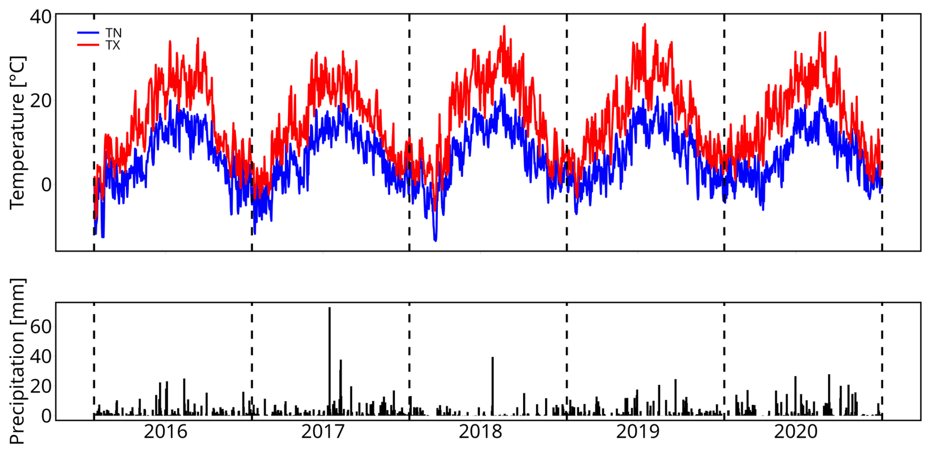
Figure 1 Evolution of meteorological conditions over the period 2016–2020: daily maximal temperature (TX, in °C), daily minimal temperature (TN, in °C), and daily cumulative precipitation (black bars, in mm). The data come from the German weather station at Berlin Schönefeld Airport (BSCH; ID: 00427).

The site has been in operation since mid-2014. This study focuses on the period 2016–2020, for which a very comprehensive dataset is available. According to the Köppen climate classification (Köppen, 1900), Berlin is located in a region of temperate oceanic climate (Cfb). Winters are cold, and summers are warm and humid. The rainfall pattern indicates moderate rainfall throughout the year (annual average of 591 mm according to Lorenz et al., 2019), with climatological maxima in June and July. Snowfall is typical from December to March. Figure 1 presents the monthly values for the daily minimum and maximum temperatures (TN and TX, respectively) and precipitation for the period of interest. The 5 years selected show contrasting meteorological conditions with a noticeable inter-annual variability in temperature and precipitation. The year 2018 was a particularly dry year, with total rainfall well below normal (only 66 mm recorded in summer compared to 157 mm on average for summer for the entire period), and also slightly warmer (average summer TX of 26.0 °C, compared to 25.0 °C on average for all the period). The year 2019 was also slightly drier and, above all, warmer than average (120 mm of precipitation and average TX of 26.4 °C in summer). In contrast, 2017 was wetter and colder in summer (268 mm of precipitation and an average TX of 23.5 °C).

3 Model description and implementation

3.1  Overview of the TEB urban canopy model

The Town Energy Balance (TEB) model is integrated in the open-access SURFEX land surface modelling platform (Masson et al., 2013) together with other dedicated surface models such as ISBA for vegetation and natural soils (Noilhan and Planton, 1989; Noilhan and Mahfouf, 1996) and FLake for inland waters (Mironov et al., 2010).

The TEB model is a surface scheme developed by Masson (2000) to represent heat, water, and momentum exchanges between urban surfaces and the atmosphere and to compute street-level microclimatic conditions. TEB can be run at street or city scale with meteorological forcings or coupled to an atmospheric model due to its simplified geometry.

In TEB, the urban geometry is represented by the concept of street canyon (Oke, 1987). This hypothesis considers that urban areas can be roughly represented as a single road between two facing buildings of the same height and infinite length and with flat roofs. With this geometry, the model computes the radiation, energy, and water balances on each surface of the street canyon (wall, road, and roof) and aggregates the fluxes to simulate the exchanges between the overall urban canopy layer and the atmosphere above. To better describe the heterogeneity of the urban environment in TEB, the interactions between urban vegetation (i.e. ground vegetation and street trees) and built-up surfaces are now represented within the street canyon (Lemonsu et al., 2012; Redon et al., 2017, 2020). To model the functioning of urban vegetation, TEB relies on the Interactions between Soil–Biosphere–Atmosphere (ISBA) model.

3.2 Initial version of the TEB-GREENROOF module

The TEB-GREENROOF module (De Munck et al., 2013) was developed in TEB to allow for the simulation of extensive green roofs. It is also based on the physics of ISBA in order to describe the soil and vegetation layers of the green roof and model its hydrological and thermal performances in interacting with the building on which it is installed, as well as exchanges with the atmosphere above. Figure 2 shows the different fluxes simulated by the original version of TEB-GREENROOF for the hydrological and thermal processes (panels a and b). At surface level, the thermal balance is estimated according to the following equation:

$$\begin{array}{}\text{(1)}& c_{\mathrm{s}}{\displaystyle \frac{\partial T_{\mathrm{S}}}{\partial t}}=Q^{*}-H-LE-G_{\mathrm{0}},\end{array}$$

where Q^* is the net radiation (W m⁻²), H is the sensible heat flux (W m⁻²), LE is the latent heat flux (W m⁻²), G₀ is the surface ground heat flux (W m⁻²), c_s is the surface soil heat capacity ($\mathrm{J}{\mathrm{K}}^{-\mathrm{1}}{\mathrm{m}}^{-\mathrm{3}}$), and T_s is the surface temperature (K).

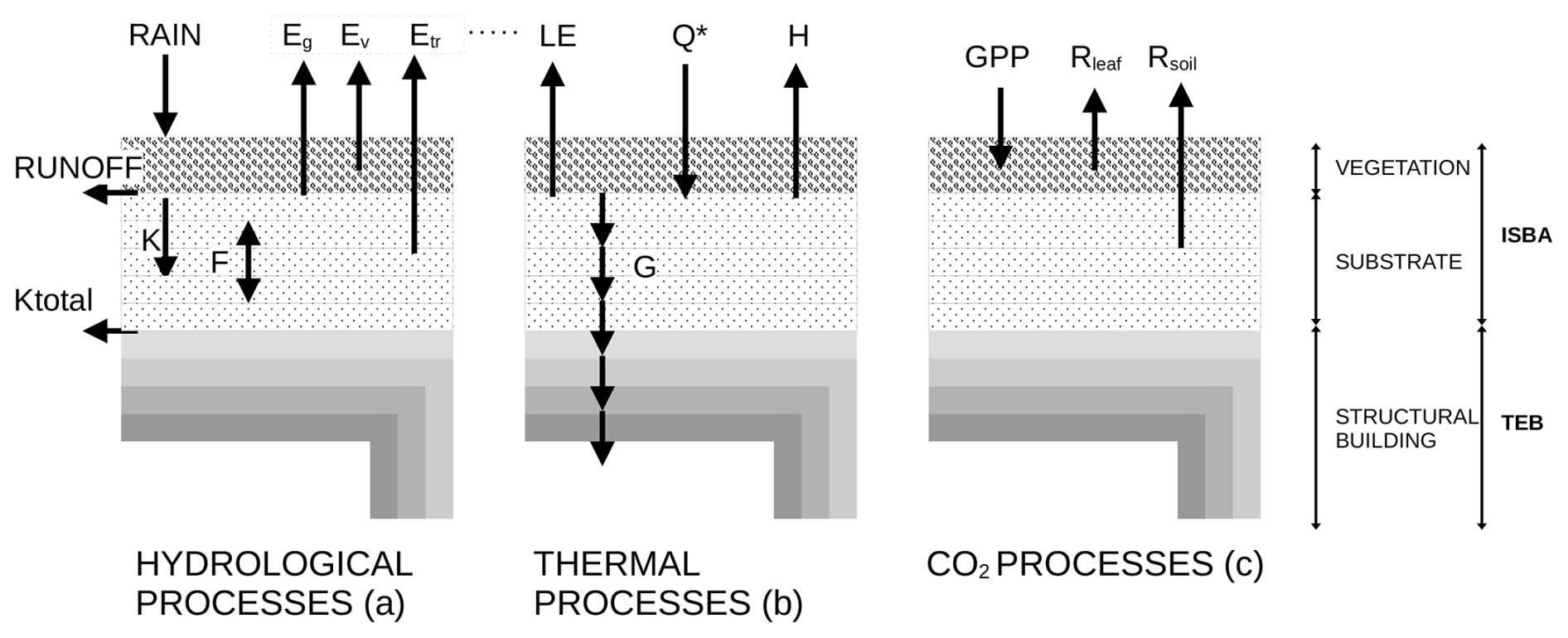
Figure 2 (a) TEB-GREENROOF hydrological processes: water gain from precipitation (RAIN), surface runoff (RUNOFF), drainage (K), total drainage (K_total), vertical water fluxes (F), ground evaporation (E_g), evaporation of water intercepted by vegetation (E_V), and vegetation transpiration (E_tr), all in $\mathrm{kg}{\mathrm{m}}^{-\mathrm{2}}{\mathrm{s}}^{-\mathrm{1}}$. (b) TEB-GREENROOF thermal processes: net radiation (Q^*), latent heat flux (LE), sensible heat flux (H), and ground heat flux (G), all in W m⁻². (c) TEB-GREENROOF CO₂ processes: gross primary production (GPP) by photosynthesis, leaf respiration (R_leaf), and soil respiration (R_soil).

The thermal balance connects to the water balance through the latent heat flux (LE). The evaporation on the vegetated surface E is the sum of the evaporation of the soil (E_g) and the evaporation of the vegetation (E_veg), $E=E_{\mathrm{g}}+E_{\text{veg}}$. The evaporation due to vegetation is also split into direct evaporation E_V from the fraction δ of the foliage covered by intercepted water and transpiration E_tr of the remaining part of the leaves ($E_{\text{veg}}=E_{\mathrm{v}}+E_{\text{tr}}$). E_g, E_V, and E_tr are calculated with the following ISBA parameterization:

$$\begin{array}{}\text{(2)}& {\displaystyle }{E}_{\mathrm{g}}=(\mathrm{1}-F_{\text{veg}})\cdot {\mathit{\rho }}_{\mathrm{a}}{C}_{\mathrm{H}}{V}_{\mathrm{a}}\left(\mathit{\alpha }{q}_{\text{sat}}\right(T_{\mathrm{s}})-q_{\mathrm{a}}),\text{(3)}& {\displaystyle }{E}_{\mathrm{v}}=F_{\text{veg}}\cdot {\mathit{\rho }}_{\mathrm{a}}\left({\displaystyle \frac{\mathit{\delta }}{R_{\mathrm{a}}}}\right)\left(q_{\text{sat}}\right(T_{\mathrm{s}})-q_{\mathrm{a}}),\text{(4)}& {\displaystyle }{E}_{\text{tr}}=F_{\text{veg}}\cdot {\mathit{\rho }}_{\mathrm{a}}\left({\displaystyle \frac{\mathrm{1}-\mathit{\delta }}{R_{\mathrm{a}}+R_{\mathrm{s}}}}\right)\left(q_{\text{sat}}\right(T_{\mathrm{s}})-q_{\mathrm{a}}),\end{array}$$

where F_veg is the fraction of vegetation, ρ_a is the air density (kg m⁻³), C_H is the turbulent exchange coefficient ($\mathrm{kg}{\mathrm{m}}^{-\mathrm{1}}{\mathrm{s}}^{-\mathrm{1}}$), V_a is the wind speed (m s⁻¹), q_sat(T_s) (kg kg⁻¹) is the saturated specific humidity at the temperature T_s, q_a is the atmospheric specific humidity at the lowest atmospheric level (kg kg⁻¹), and α is a coefficient that depends on soil moisture. $R_{\mathrm{a}}=(C_{\mathrm{H}}{V}_{\mathrm{a}}{)}^{-\mathrm{1}}$ is the aerodynamic resistance and R_s the canopy surface resistance that depend on atmospheric factors, soil water content, and LAI, which are modelled later with the implementation of CO₂ fluxes.

The soil of the green roof is described using the multi-layer diffusion version ISBA-DF (Boone et al., 2000; Decharme et al., 2011), which discretizes the soil into different vertical layers. In each soil layer, the evolution equation of soil temperature is given by the following expression:

$$\begin{array}{}\text{(5)}& c_{\mathrm{g}}{\displaystyle \frac{\partial T}{\partial t}}={\displaystyle \frac{\partial G}{\partial z}}+\mathit{\varphi },\end{array}$$

where T is the soil temperature (K), G is the vertical ground heat flux ($\mathrm{J}{\mathrm{m}}^{-\mathrm{2}}{\mathrm{s}}^{-\mathrm{1}}$), c_g is the soil heat capacity ($\mathrm{J}{\mathrm{K}}^{-\mathrm{1}}{\mathrm{m}}^{-\mathrm{3}}$), ϕ is a latent heat source/sink resulting from phase transformation of soil water ($\mathrm{J}{\mathrm{m}}^{-\mathrm{3}}{\mathrm{s}}^{-\mathrm{1}}$), and z is the soil depth (m).

For the evolution of soil liquid water and soil ice volumetric content (m³ m⁻³), the equations are

$$\begin{array}{}\text{(6)}& {\displaystyle \frac{\partial w_{\mathrm{l}}}{\partial t}}=-{\displaystyle \frac{\partial F}{\partial z}}-{\displaystyle \frac{\mathit{\varphi }}{L_{\mathrm{f}}{\mathit{\rho }}_{\mathrm{w}}}}-{\displaystyle \frac{S_{\mathrm{l}}}{{\mathit{\rho }}_{\mathrm{w}}}}(w_{\text{min}}\le w_{\mathrm{l}}\le w_{\text{sat}}),\text{(7)}& {\displaystyle \frac{\partial w_{\mathrm{i}}}{\partial t}}={\displaystyle \frac{\mathit{\varphi }}{L_{\mathrm{f}}{\mathit{\rho }}_{\mathrm{w}}}}(\mathrm{0}\le w_{\mathrm{i}}\le w_{\text{sat}}-w_{\text{min}}),\end{array}$$

where F is the vertical water flux (m s⁻¹), L_f is the latent heat of water fusion (J kg⁻¹), ρ_w is the liquid water density (kg m⁻³), and S_l represents external sources/sinks for liquid water ($\mathrm{kg}{\mathrm{m}}^{-\mathrm{3}}{\mathrm{s}}^{-\mathrm{1}}$).

In the soil, the hydrological and thermal balances are coupled through the effective thermal properties of each soil layer j, which change over time as a function of the soil water content. This is the case for both the layer-averaged soil heat capacity (c_g j, in $\mathrm{J}{\mathrm{K}}^{-\mathrm{1}}{\mathrm{m}}^{-\mathrm{3}}$) and thermal conductivity (λ_j, in $\mathrm{kg}\mathrm{m}{\mathrm{s}}^{-\mathrm{3}}{\mathrm{K}}^{-\mathrm{1}}$) for layer j, according to

$$\begin{array}{}\text{(8)}& {\displaystyle }{c}_{\mathrm{g}j}=(\mathrm{1}-w_{\text{sat}j})c_{\text{dry}j}+w_{\mathrm{l}j}{c}_{\mathrm{l}}+w_{\mathrm{i}j}{c}_{\mathrm{i}},\text{(9)}& {\displaystyle }{\mathit{\lambda }}_j=K_{\mathrm{e}}{\mathit{\lambda }}_{\text{sat}j}+(\mathrm{1}-K_{\mathrm{e}}){\mathit{\lambda }}_{\text{dry}j},\end{array}$$

where w_l j and w_i j are the soil liquid water content and soil ice content in layer j (m³ m⁻³). c_dry j is the heat capacity of the dry-soil matrix for layer j, and c_l and c_i are the heat capacities of liquid water and ice, respectively. K_e is the Kersten number (that is, a dimensionless parameter representing the normalized thermal conductivity as a function of the degree of saturation only), and λ_sat j and λ_dry j are the saturated and dry-soil thermal conductivities for layer j, respectively.

3.3 Implementation of CO₂ fluxes in TEB-GREENROOF

Similar to the formulation of radiative, thermal, and hydrological exchanges, CO₂ fluxes in TEB-GREENROOF are adapted from an existing module in ISBA, and the CO₂ fluxes are modelled in TEB-GREENROOF by activating, with some adaptations, an existing module of ISBA designed to represent C fluxes in vegetation and soils.

The main fluxes are plant photosynthesis (or gross primary production, referred to as GPP, in $\mathrm{g}\mathrm{C}{\mathrm{m}}^{-\mathrm{2}}{\mathrm{yr}}^{-\mathrm{1}}$) and ecosystem respiration (R_ECO, in $\mathrm{g}\mathrm{C}{\mathrm{m}}^{-\mathrm{2}}{\mathrm{yr}}^{-\mathrm{1}}$), which combine leaf respiration (R_leaf, in $\mathrm{g}\mathrm{C}{\mathrm{m}}^{-\mathrm{2}}{\mathrm{yr}}^{-\mathrm{1}}$ from Eqs. B10–B11) and soil heterotrophic respiration (R_soil, in $\mathrm{g}\mathrm{C}{\mathrm{m}}^{-\mathrm{2}}{\mathrm{yr}}^{-\mathrm{1}}$) (see Fig. 2c). The difference between these two large fluxes is defined as the net ecosystem exchange, $\text{NEE}=R_{\text{ECO}}-\text{GPP}$ (Bonan, 2016). Photosynthesis and leaf respiration are modelled with the A-gs parameterization (Calvet et al., 1998, 2004), based on the assimilation scheme proposed by Jacobs (Jacobs, 1994; Goudriaan et al., 1985) (see Appendix B). This semi-empirical model has the advantage of being simple and suited for both C₃ and C₄, the most prominent physiological plant groups based on different photosynthetic pathways. The approach chosen considers that light and CO₂ atmospheric concentration are the two limiting factors impacting the net photosynthetic rate.

The goal of this study is to adapt some aspects of the present parameterization in order to model Berlin Brandenburg Airport's extensive green roof by representing the behaviour of the dominant Sedum species (which is widely used for extensive green roofs). Sedum are facultative C₃–CAM (crassulacean acid metabolism) (Winter, 2019), meaning that they behave like a C₃ plant when they are well watered and switch to a CAM photosynthesis pathway when they lack water. With CAM behaviour, the stomata of the plant open only at night to fix CO₂. The photosynthesis takes place during the day, requiring light energy, but the leaf stomata remain closed to prevent water loss through evapotranspiration. Nonetheless, the flux measurements carried out on the green roof at Berlin Brandenburg Airport did not reveal any periods with CAM behaviour, which would be characterized by the absorption of CO₂ during the night. Consequently, the question of modelling the photosynthesis mechanisms specific to this particular species in the ISBA model (which does not include CAM behaviour like most large-scale vegetation models) was not investigated further in this study. However, it still requires adaptation of the model with a specific parameterization to match the behaviour of Sedum on a shallow substrate.

First, the maximum net CO₂ assimilation (A_m,max, in $\mathrm{g}{\mathrm{m}}^{-\mathrm{2}}{\mathrm{s}}^{-\mathrm{1}}$) and the mesophyll conductance ($g_{\text{mes}}^{*}$, in m s⁻¹) use inhibition functions (see Appendix Eqs. A2–A3) with reference temperature adjusted to better represent optimum temperature. This was done to differentiate optimum assimilation between C₃ and C₄ plants. However, an analysis of the observed CO₂ fluxes measured by eddy covariance did not show any high- or low-temperature inhibition of photosynthesis in the range of temperatures observed. Because we could not find data triggering high- and low-temperature inhibition for these species, we decided to set the inhibition functions to 1, which modifies the equations for A_m,max and g_mes:

$$\begin{array}{}\text{(10)}& {\displaystyle }{A}_{m,\text{max}}\left(T_{\mathrm{s}}\right)=A_{m,\text{max}}\left(\mathrm{25}\right)\cdot Q_{\mathrm{10}}^{\frac{T_{\mathrm{s}}-\mathrm{25}}{\mathrm{10}}},\text{(11)}& {\displaystyle }{g}_{\text{mes}}^{*}\left(T_{\mathrm{s}}\right)=g_{\text{mes}}^{*}\left(\mathrm{25}\right)\cdot Q_{\mathrm{10}}^{\frac{T_{\mathrm{s}}-\mathrm{25}}{\mathrm{10}}},\end{array}$$

where A_m,max(25) is the maximum net CO₂ assimilation at 25 °C in $\mathrm{mg}{\mathrm{m}}^{-\mathrm{2}}{\mathrm{s}}^{-\mathrm{1}}$; T_s is the leaf skin temperature (K), here considered the first layer of soil temperature; and $g_{\text{mes}}^{*}\left(\mathrm{25}\right)$ is the mesophyll conductance at 25 °C. Q₁₀ is the response function defined as a proportional increase in a parameter for a 10° increase.

When soil moisture content drops, plants tend to close their stomata to limit water loss. This is described empirically by a soil water stress function (F2) that simply models the stomata closing and opening when the plant lacks water according to the regulation of the mesophyll conductance:

$$\begin{array}{}\text{(12)}& g_{\text{mes}}=g_{\text{mes}}^{*}\left(T_{\mathrm{s}}\right)\cdot F\mathrm{2},\end{array}$$

with the normalized soil water stress factor estimated as

$$\begin{array}{}\text{(13)}& F\mathrm{2}=\sum _{j=\mathrm{1}}^N\left[{\mathrm{{\rm Y}}}_j\cdot \left({\displaystyle \frac{w_j-w_{\text{wilt}j}}{w_{\text{fc}j}-w_{\text{wilt}j}}}\right)\right],\end{array}$$

where N is the number of soil layers, and Υ_k is the root fraction in layer j. w_wilt j is the wilting point, w_fc j the field capacity, and w_j the soil water content in layer j. As the substrate of the extensive green roof is shallow, thresholds F2_min and F2_max are prescribed for F2 to prevent photosynthesis cut or variations that are too excessive.

The respiration of the soil (in $\mathrm{kg}{\mathrm{m}}^{-\mathrm{2}}{\mathrm{s}}^{-\mathrm{1}}$) is estimated with the simple Norman et al. (1992) respiration scheme:

$$\begin{array}{ll}{\displaystyle }{R}_{\text{soil}}& {\displaystyle }=\mathrm{4.4}\times {\mathrm{10}}^{-\mathrm{8}}\times (\mathrm{13.5}+\mathrm{5.4}\cdot \text{LAI})\\ \text{(14)}& {\displaystyle }& {\displaystyle }\cdot w_{\mathrm{10}}\cdot e^{\mathrm{0.069}\cdot (T_{\mathrm{s}\mathrm{10}}-\mathrm{25}),}\end{array}$$

where LAI is the leaf area index (m² m⁻²), w₁₀ is the weighted soil volumetric water content between 0–10 cm depth (%), and T_s10 is the weighted soil temperature between 0–10 cm depth (°C). Since the soil on the green roof is very shallow, water content thresholds $w_{{\mathrm{10}}_{\text{min}}}$ and $w_{{\mathrm{10}}_{\text{max}}}$ are prescribed during the calibration to prevent extreme values.

Furthermore, the A-gs CO₂ assimilation scheme can be either forced by a prescribed LAI or coupled to a biomass scheme, making the LAI evolve over time. In the model, LAI is the variable that reflects the vegetation evolution (i.e. the CO₂ accumulation). Making the LAI evolve dynamically during the simulation, rather than prescribing LAI values imposed on the model, enables us to represent the impact of meteorological conditions on vegetation over the long term and thus to simulate more realistic CO₂ accumulation scenarios over longer periods.

We use the ISBA NIT (Calvet and Soussana, 2001) biomass scheme that only represents above-ground biomass, separated into three different reservoirs: a leaf biomass reservoir, an above-ground stem biomass reservoir, and a residual reservoir.

Each biomass reservoir (B_i, expressed in kg of dry matter (DM) m⁻²) follows the same time evolution equation, the principle of which can be expressed as follows (Garisoain, 2023):

$$\begin{array}{}\text{(15)}& {\displaystyle \frac{\mathrm{\Delta }{B}_{\mathrm{i}}}{\mathrm{\Delta }t}}=A_{\mathrm{i}}-D_{\mathrm{i}}-R_{\mathrm{i}},\end{array}$$

with A_i being the biomass input and D_i and R_i being biomass loss due to mortality, allocation to other reservoirs, and respiration. The input flux for leaf biomass is the carbon assimilation due to photosynthesis (expressed in $\mathrm{kg}\mathrm{C}{\mathrm{m}}^{-\mathrm{2}}{\mathrm{d}}^{-\mathrm{1}}$):

$$\begin{array}{}\text{(16)}& A_{\text{leaf}}=A_{\text{n,day}}\cdot \mathrm{\Delta }t.\end{array}$$

After a daily biomass iteration, the LAI is calculated from the leaf biomass and the specific leaf area (SLA; in m² per kg DM) as follows:

$$\begin{array}{}\text{(17)}& \text{LAI}=\text{SLA}\cdot B_{\text{leaf}}.\end{array}$$

Except for crops, ISBA assumes a constant vegetation cover with time. However, extensive green roof vegetation can be patchy, and the vegetation cover may vary in time. To take this heterogeneity and variability into account, the fraction of vegetation cover is estimated by fitting the equation on the estimation of LAI and vegetation cover:

$$\begin{array}{}\text{(18)}& F_{\text{veg}}=\mathrm{1}-e^{a\cdot \text{LAI}},\end{array}$$

where a is a coefficient set on the basis of observations.

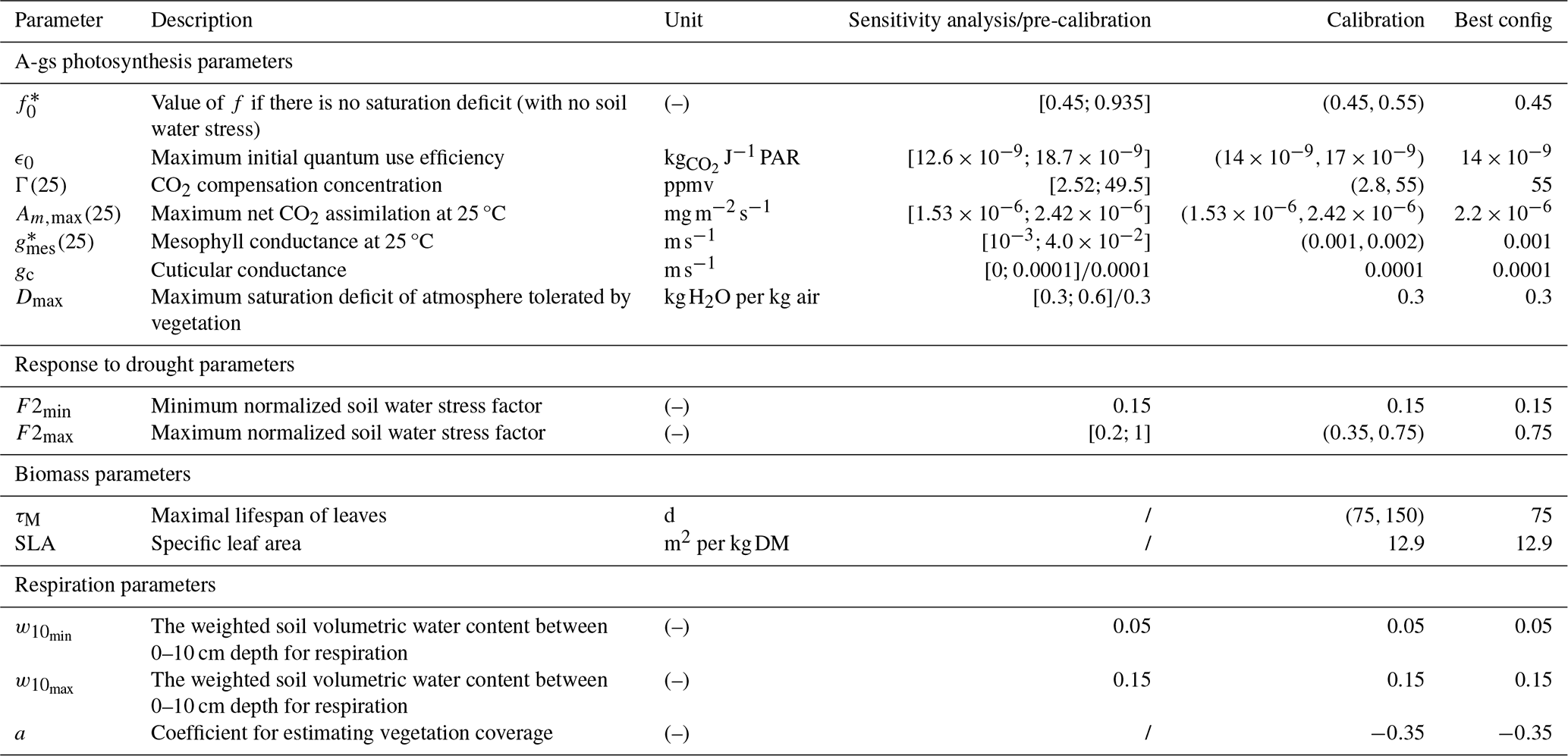
All the vegetation parameters required for the CO₂ flux modelling are listed in Table 2. Standard values are available in ISBA for each of these parameters, for both C₃ and C₄ plants (Gibelin et al., 2006). Since it is challenging to find appropriate ecophysiological data to derive these parameter values for Sedum, we chose to calibrate some of them in Sect. 5.

4 Configuration of TEB simulation

4.1 Atmospheric conditions

In this study, TEB is run in an offline simulation configuration over 5 years, from 2016 to 2021. It is applied to a single grid point, i.e. for an average urban canyon whose characteristics are representative of the study site, in particular the properties of the green roof. In offline mode, the time evolution of atmospheric conditions over the urban canyon must be provided to the TEB model at both the given altitude and the time step. The data required are the above urban canopy air temperature, humidity, pressure, and CO₂ concentration; the wind speed and direction; precipitation; and the short-wave (direct and scattered) and long-wave incoming radiation.

Here, the meteorological forcing is built with local observations described in Sect. 2 and provided to the model with a time resolution of 30 min. The specific humidity is calculated with the relative humidity, air pressure, and air temperature measurements. The partitioning of the incoming global short-wave radiation into scattered and direct components is made based on the method of Erbs et al. (1982). Solid and liquid precipitation rates are determined by disaggregating the total precipitation, first according to the rain/snow precipitation classification directly provided from the nearby German Weather Service station at Berlin Schönefeld Airport (BSCH; ID: 00427). When classification data are missing or indicate rain and snow during the same day, disaggregation is done using the air temperature recorded on the roof by applying a threshold of 273.15 K.

4.2 TEB model configuration

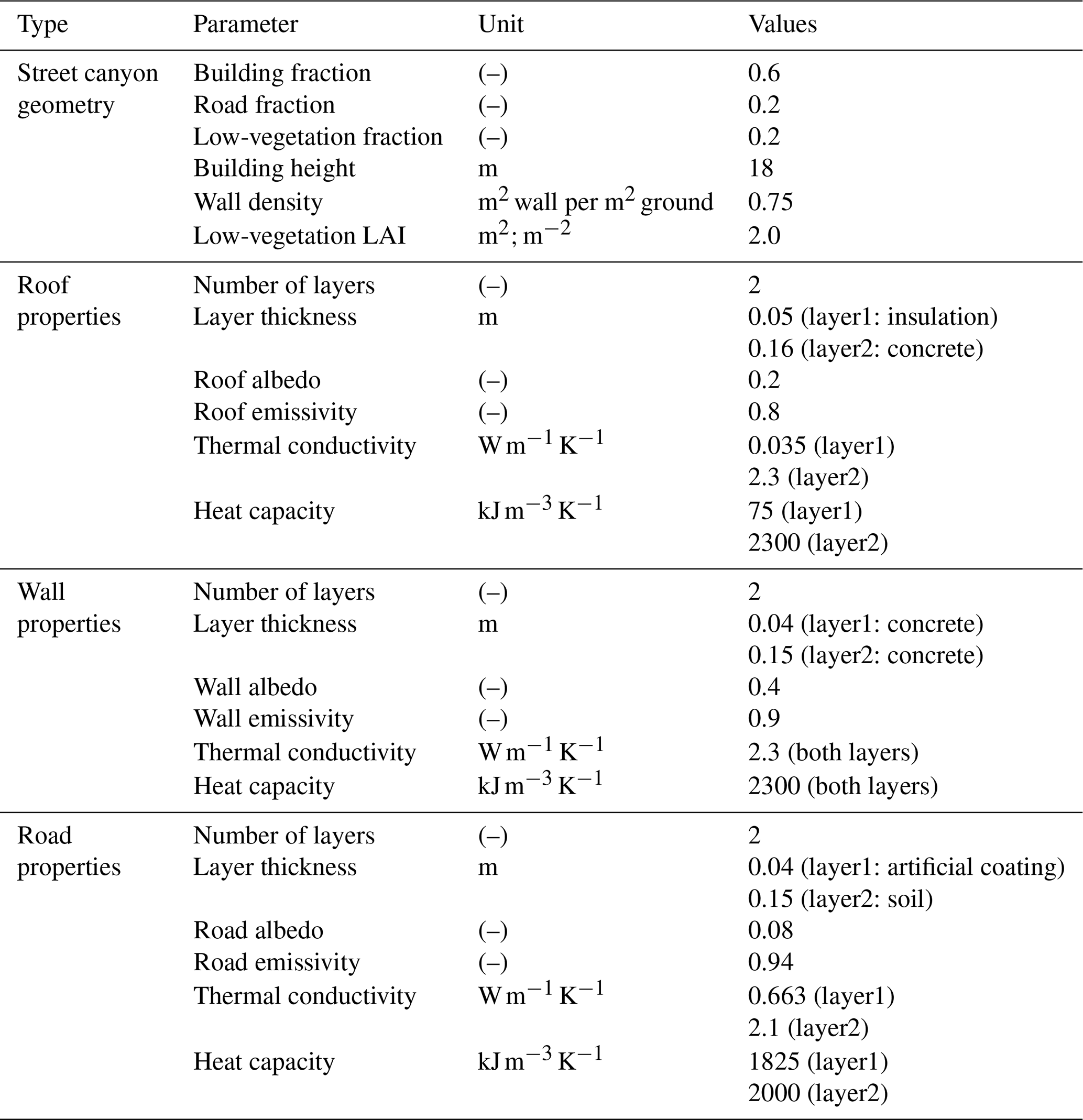
The TEB model is run on a 1D grid, with the urban canyon dimensions and properties defined as the average parameters of the measuring site. The height of the building is set to 18 m, which is consistent with the airport parking lot characteristics. The forcing height is determined according to the sensor location on the green roof, i.e. 19.15 m above ground level (a.g.l.) for wind speed and direction and 20 $\mathrm{m}\mathrm{a}.\mathrm{g}.\mathrm{l}.$ for air temperature and humidity. TEB runs with a simplified surface-boundary-layer scheme (Hamdi and Masson, 2008; Masson and Seity, 2009), allowing for the vertical discretization of the atmosphere in the canyon (from the ground to the forcing height) into six layers of microclimate variables. The fraction of building is set to 0.6 and fully covered by green roofs using the TEB-GREENROOF module, the fraction of road is 0.2, and the fraction of low vegetation is 0.2 with the GARDEN module (Lemonsu et al., 2012). The road is discretized into two layers, corresponding to a surface layer of artificial coating and a basement layer of natural soil. The parking lot is a concrete building with large openings on the facades. The walls are defined in the model as having two layers of concrete, and the roof consists of a surface layer of concrete and a second layer of insulation.

Table 1 TEB-GREENROOF input parameters for green roof substrate and vegetation. Geometric parameters are defined according to the soil depth of the site; surface and thermal properties are based on the previous study of De Munck et al. (2013), with an adjustment to soil thermal conductivity. For hydrological properties, B_coef is set based on De Munck et al. (2013); the wilting point, field capacity, and porosity profile are derived from soil water content measurements; the saturated soil matrix is defined on the basis of ex situ analysis; and saturated hydraulic conductivity is based on soil manufacturer documentation.

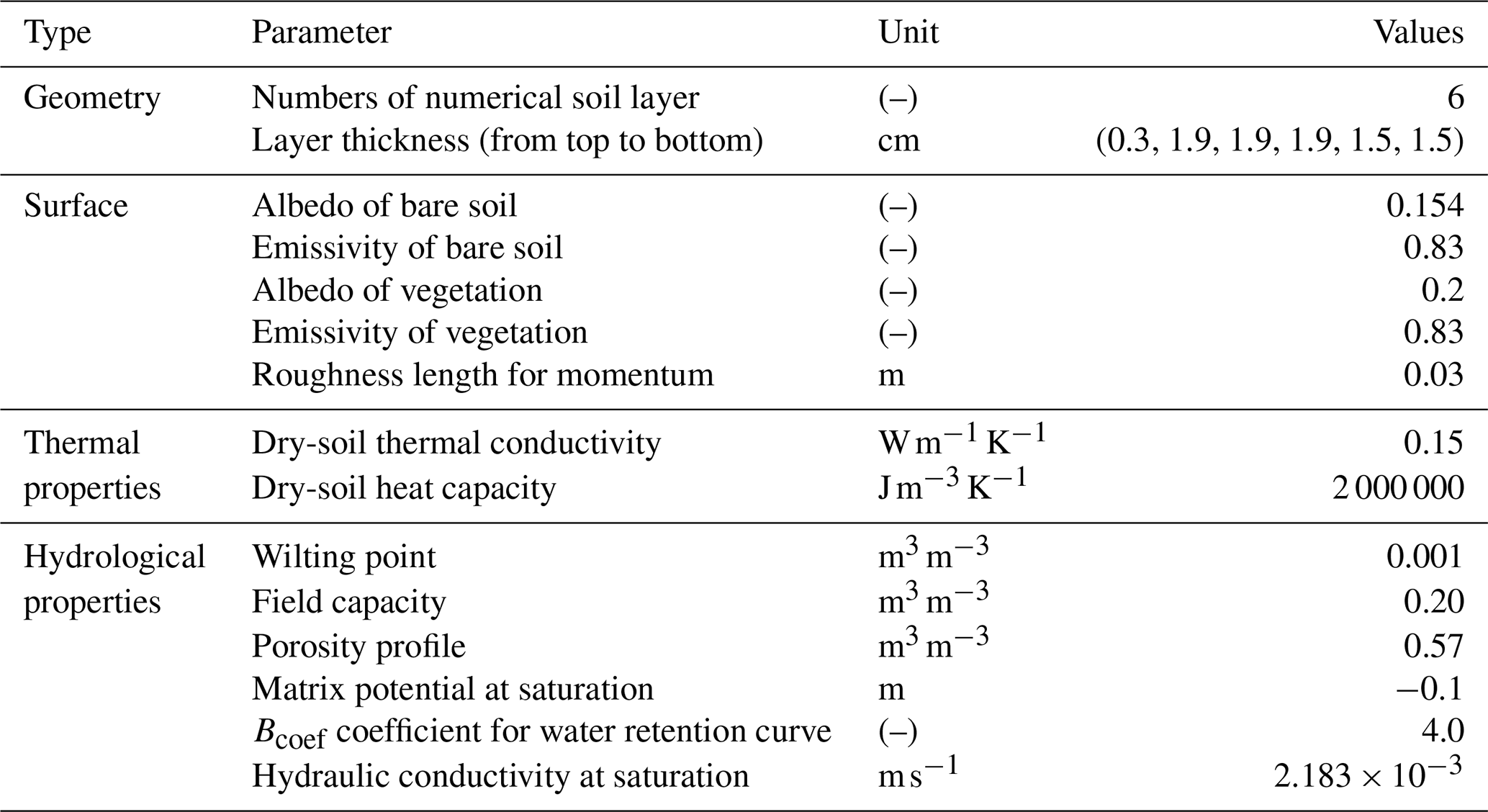
Table 2 Description of the input parameters for the calculation of CO₂ fluxes in TEB-GREENROOF. All the parameter values tested for the sensitivity analysis, pre-calibration, and final calibration stages are listed. The data in square brackets define the ranges of values tested, and the data in brackets define the pairs of values tested.

Besides the photosynthesis parameters (described in Table 2), the input parameters of the TEB-GREENROOF module, including the description of the green roof and the thermal and hydrological properties, are described in Table 1. The green roof soil is discretized into six layers with the same composition for a total depth of 0.09 m. With regard to hydrological properties, the potential of the soil matrix at saturation is defined based on ex situ analysis. The empirical coefficient for the water retention curve (B_coef) varies according to soil and connects the water potential to the water content in a soil matrix derived by Clapp and Hornberger (1978). It is set based on the results of a previous case study referenced in De Munck et al. (2013). The hydraulic conductivity at saturation is based on the soil manufacturer's documentation. The soil porosity profile, field capacity, and wilting point are set directly based on measurements of soil water content on the green roof. The definition of the thermal properties is based on the initial calibration proposed by De Munck et al. (2013) for a different instrumented extensive green roof: the same value of dry-soil heat capacity is applied, but the dry-soil thermal conductivity is slightly increased to better model the heat conduction in the soil according to measurements (not presented here). The vegetation albedo and emissivity are taken from the previous study of De Munck et al. (2013).

5 Definition of green roof CO₂ flux parameters

Without information on the specific characteristics of the current green roof to be simulated, the input parameters for the photosynthesis model must be defined. The initialization of these parameters is done following three successive steps:

1. Sensitivity analysis on the main parameters of the A-gs photosynthesis model. This step is based on a standalone and very low computing time version of A-gs (detailed in Appendix C). Forced by predefined microclimate conditions, a very large number of simulations are carried out to test a wide range of parameter values and clarify which parameters are the most significant and have the greatest effect on the calculation of CO₂ fluxes.

2. Pre-calibration. This step consists of running additional simulations, again using the standalone version of A-gs but with a focus on the parameters selected in the previous step in order to narrow the range of plausible values (Appendix E).

3. Calibration of the selected parameters according to the values identified in the previous step. This time, several combinations of plausible parameter values are tested by running the full TEB configuration considering dynamic LAI. Based on these simulations, the best configuration can be identified.

5.1 Sensitivity analysis of ISBA–A-gs parameters

5.1.1 Sobol index method

In order to assess which ISBA–A-gs parameters are the most predominant in modelling carbon uptake, a global sensitivity analysis is performed on the parameters listed in Table 2. The approach used is the Sobol method (Sobol, 1993, 2001) that can be applied for either linear or non-linear models. Two indices are considered here. The first one, S_i, is the first-order global sensitivity of output Y to a single selected input parameter X_i, i.e. the variance of Y when X_i is the only parameter that varies. S_i is normalized by the variance of Y to obtain a score between 0 (no sensitivity) and 1 (full sensitivity). The second index considered, $S_{T_{\mathrm{i}}}$, also known as the total-order index, calculates the variance of output Y to X_i when X_i varies with the other parameters in every possible combination (X_i varies solely, then X_i varies with each parameter, then three parameters including X_i vary together, etc.). As for S_i, $S_{T_{\mathrm{i}}}$ is normalized by the variance of Y with a score between 0 (no sensitivity) and 1.

To compute these two indices for each A-gs parameter, we use a Monte Carlo approach developed by Saltelli et al. (2010). This involves working with samplings that adequately span the space of possible values for each parameter. In this study, the sampling is performed with Latin hypercube sampling (Stein, 1987), which is a stratified sampling method aiming to spread the sample points evenly across all possible values. This is done using the R package “lhs” (Carnell, 2022) with the geneticLHS method (Stocki, 2005), which samples using a genetic algorithm to maximize the mean distance from each point to all other points. The complete sensitivity analysis process is summarized in Fig. 3.

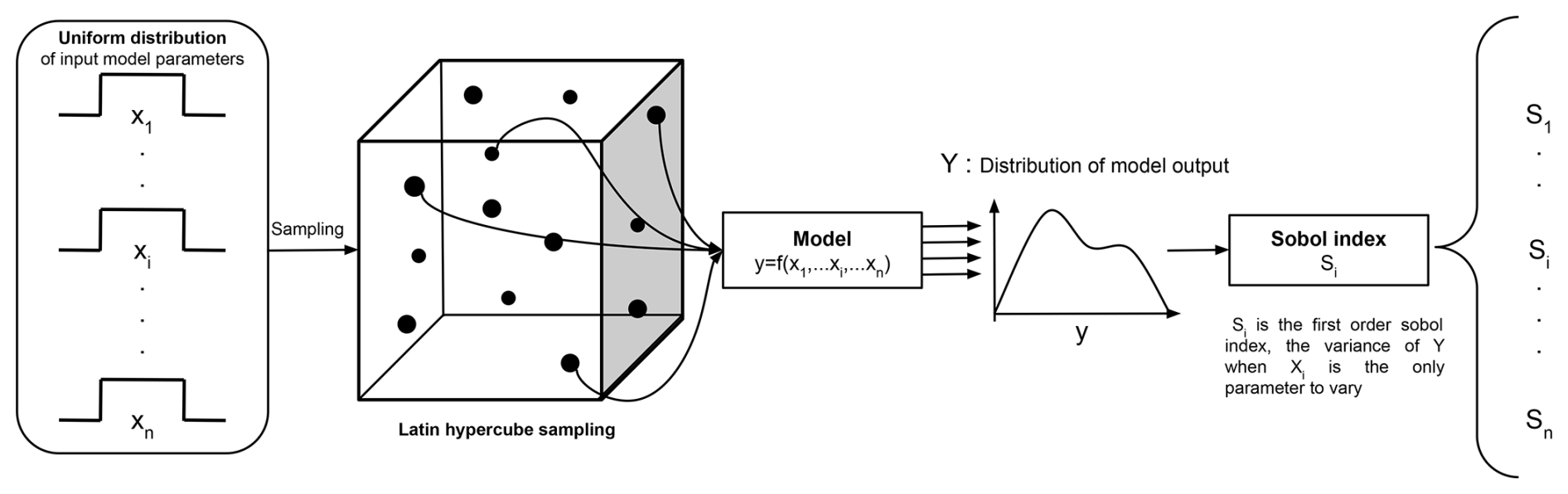
Figure 3 Flowchart of sensitivity analysis. This chart is for the first order only and is the same for the total effect index, except for the calculation of the Sobol index box.

5.1.2 Application to the photosynthesis A-gs model

To implement this sensitivity study on the input parameters of the A-gs photosynthesis model, a simplified modelling configuration is developed. The sensitivity analysis is carried out with the standalone A-gs model (Appendix C) on scores of simulated CO₂ fluxes. The mean absolute error (MAE) and root-mean-square error (RMSE) are computed over the 5 years of observations selected at a temporal scale of 30 min. Among all input parameters of the A-gs model, eight parameters (Table 2) are not set on observations and are selected for the sensitivity analysis. This includes $g_{\text{mes}}^{*}\left(\mathrm{25}\right)$ and A_m,max(25) presented in Sect. 3.3, with the cuticular conductance (g_c), the maximum saturation deficit of the atmosphere tolerated by vegetation (D_max), the maximum initial quantum use efficiency (ϵ₀), the ${}_{{\mathrm{CO}}_{\mathrm{2}}}$ compensation concentration (Γ(25)), the value of the f factor when there is no saturation deficit ($f_{\mathrm{0}}^{*}$), and the maximum normalized soil water stress factor (F2_max). The range of values for part of the parameters is based on a previous sensitivity analysis from Aouade et al. (2020) with reference values from the literature: $g_{\text{mes}}^{*}\left(\mathrm{25}\right)$ from Calvet (2000), g_c from Gibelin et al. (2006), and D_max from Calvet (2000). For the other parameters, the ranges are set according to the default values defined for types C₃ and C₄ in ISBA–A-gs, with a ±10 % margin: ϵ₀, Γ(25), and A_m,max(25) from Gibelin et al. (2006) and $f_{\mathrm{0}}^{*}$ from Jacobs (1994). The parameters and associated value ranges are listed in Table 2. The distribution within the fixed range of each parameter is defined according to a uniform distribution.

The size of each sampling matrix (the number of different values for one parameter) is set to 5000, which implies a total of 50 000 simulations based on the Monte Carlo method. Here, the output variables of interest for which the Sobol indices are calculated are the mean absolute error (MAE) and the root-mean-square error (RMSE) of the net CO₂ fluxes simulated by A-gs compared with the net CO₂ flux measurements collected on the instrumented green roof.

5.1.3 Sensitivity analysis results

The results of the sensitivity analysis on the A-gs input parameters for its implementation in the TEB-GREENROOF model for CO₂ calculation are presented in Fig. 4 for both MAE and RMSE. The values obtained for the Sobol index make it possible to first identify the parameters with no influence on the net carbon flux scores, i.e. D_max and g_c. As a result, they are set to default values, as listed in Table 2. All other parameters are retained for the calibration with the same range for the pre-calibration. Among them, $g_{\text{mes}}^{*}\left(\mathrm{25}\right)$ is the most sensitive one, followed by Γ(25) and ϵ₀, with similar results for MAE and RMSE. As a result, these three input parameters have the greatest influence on the performance of the A-gs model in calculating CO₂ fluxes and thus require more meticulous calibration (presented in the next section). The parameters A_m,max(25), $f_{\mathrm{0}}^{*}$, and F2_max have a smaller but non-negligible impact so that they are also retained for the pre-calibration.

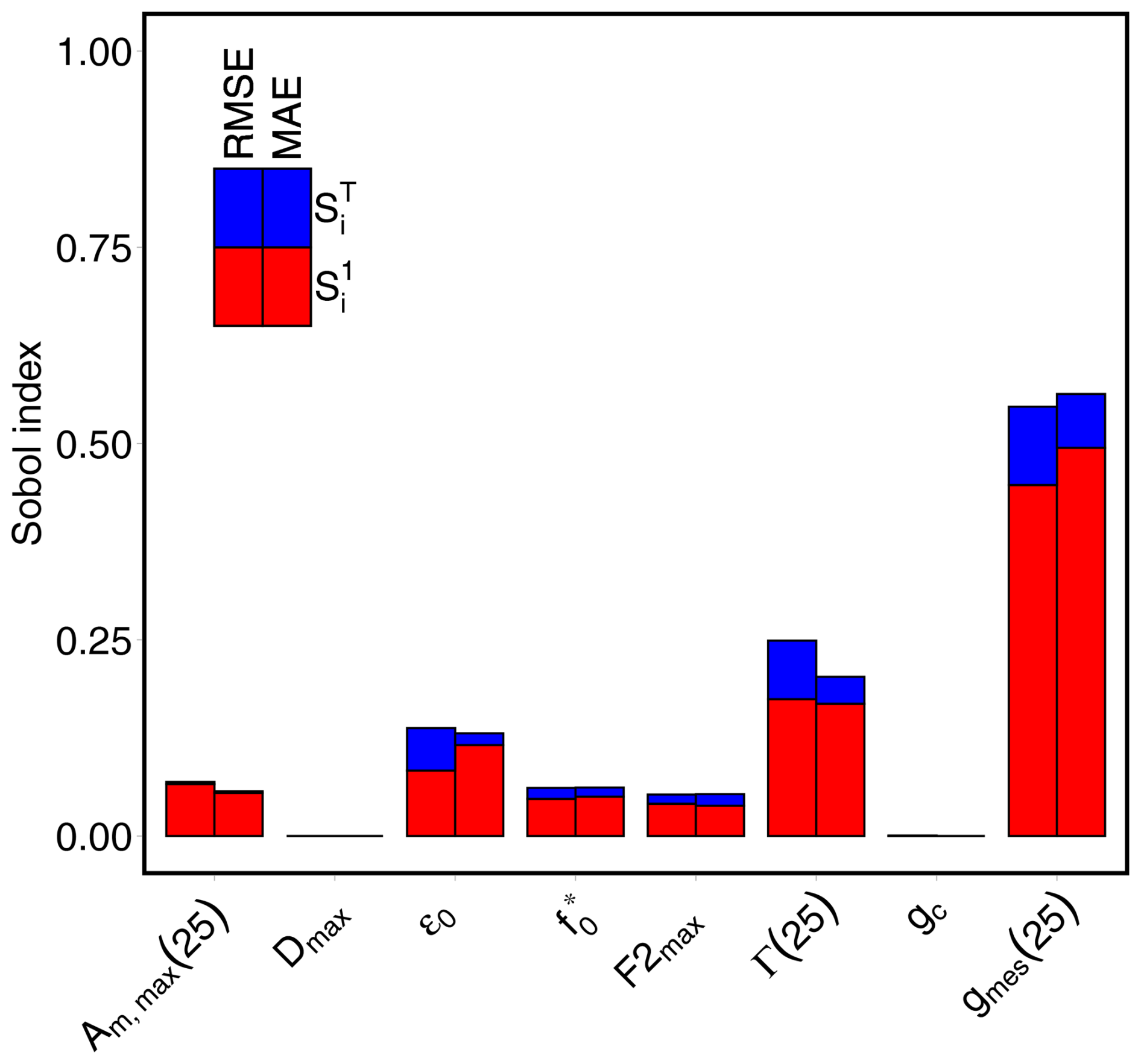
Figure 4 Comparison of the Sobol first-order (red) and total-order (blue) indexes calculated for the eight variables in the sensitivity analysis, for both RMSE (left bar) and MAE (right bar).

5.2 Calibration of A-gs parameters

5.2.1 Method

The model is calibrated based on the observation dataset of net CO₂ fluxes divided into two distinct time periods: a 4-year calibration period (from 2016 to 2019) and a 1-year evaluation period (2020). Pre-calibration (Appendix E) is done to reduce the range of values for the six photosynthesis parameters to be calibrated ($g_{\text{mes}}^{*}\left(\mathrm{25}\right)$, Γ(25) ϵ₀, A_m,max(25), $f_{\mathrm{0}}^{*}$, and F2_max).

An ensemble of TEB-GREENROOF simulations is then run according to the full configuration presented in Sect. 4.2 (and considering a dynamic LAI). Each simulation represents a different combination of parameter values. For each of the six photosynthesis parameters, two values are tested based on the pre-calibration results (Table 2). Since TEB-GREENROOF simulations are performed with a dynamic LAI, additional parameters related to the biomass evolution need to be calibrated, i.e. the maximal lifespan of leaves (τ_M) and the specific leaf area (SLA). For Sedum album, the value of SLA is set to 12.9 m² per kg DM according to the TRY database (Kattge et al., 2020), which brings together the different plant trait databases worldwide (the last version of TRY contains more than 1 million trait records for 6.24 million individual plants). The parameter τ_M is tested for the two values of 75 and 150 d, with 150 being the default value in ISBA for C₃ and C₄ plants (Gibelin et al., 2006) and 75 being half of this value. In total, 128 combinations of parameters are simulated with TEB-GREENROOF. To identify the best configuration, the statistical scores of the 128 experiments calculated over 2016–2019 are compared by crossing the mean absolute error (MAE) of net CO₂ fluxes and the root-mean-square error (RMSE) of LAI.

5.2.2 Calibration results

Figure 5 illustrates the outcomes of all simulations in terms of MAE for the net CO₂ fluxes and RMSE for LAI, with details of the values of each parameter in all simulations. In accordance with the findings of the sensitivity analysis, the mesophyll conductance at 25 °C is identified as the most influential parameter. In Fig. 5c nearly all simulations with $g_{\text{mes}}^{*}\left(\mathrm{25}\right)=\mathrm{0.001}$ m s⁻¹ demonstrate better performances than simulations with $g_{\text{mes}}^{*}\left(\mathrm{25}\right)=\mathrm{0.002}$ m s⁻¹ for both net CO₂ fluxes and LAI. The maximal lifespan of leaves (τ_M) is also found to have a significant impact. However, as evidenced by the two distinct curves (Fig. 5a), this parameter primarily affects the representation of LAI, with systematically better RMSE for τ_M=75 d than for 150 d. For Γ(25) and ϵ₀ (Fig. 5d and f), the two values tested for each parameter give quite comparable performances. It is nonetheless possible to identify a single value, considered the best, set to 55 ppmv for Γ(25) and 1.4 kg CO₂ PAR for ϵ₀. For the other parameters, namely A_m,max(25), $f_{\mathrm{0}}^{*}$, and F2_max (Fig. 5b, e, and g), it is more difficult to conclude on the values leading to the best configuration. Indeed, the differences in performances between the simulations performed with the two values of A_m,max(25) are very low, which corresponds well with the sensitivity analysis results. For $f_{\mathrm{0}}^{*}$ and F2_max, the simulations with the best RMSE for LAI do not correspond to the simulations with the best MAE for CO₂ fluxes. The best configuration is highlighted in Fig. 5a, with the corresponding parameter values listed in Table 2. It is selected because it gives the best simulation for LAI and still close to the best simulation for $F_{{\mathrm{CO}}_{\mathrm{2}}}$ MAE.

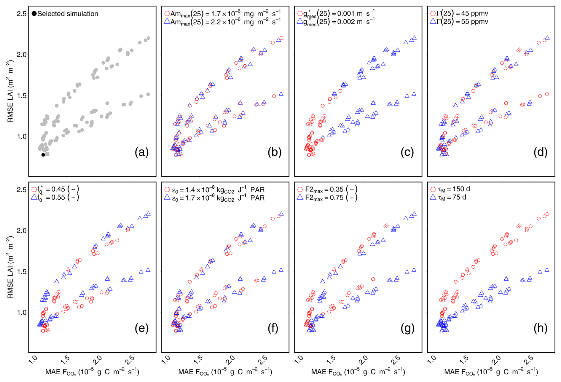
Figure 5 Comparison of the performances of the 128 simulations combining the RMSE of daily LAI (x axis) and the MAE of 30 min average instantaneous net CO₂ fluxes (y axis). Panel (a) highlights the simulation selected as the best (black dot) compared to the other simulations (grey dots). For each of the other panels corresponding to one of the variables to be calibrated (b–h), the red/blue colour code distinguishes the performance of the two values tested for that variable.

5.3 Evaluation of the TEB-GREENROOF

The final simulation (i.e. the evaluation simulation) is based on the best configuration obtained from the calibration stage, with all parameters listed in Table 2. It is analysed and evaluated here in relation to observations of LAI and CO₂ fluxes.

5.3.1 Dynamic LAI modelling

The modelling of the evolving LAI using the biomass model is presented in Fig. 6 and compared with the LAI retrieved from observations. The observed LAI was estimated by capturing the variation in the green chromatic information (green fraction) in the RGB space from photographs taken at 10 different randomly selected locations on the roof, approximately once a month (Heusinger and Weber, 2017b). Since observation-based LAI is estimated from the analysis of discontinuous photographs, it is difficult to assess the accuracy of the model in detail. Nevertheless, some interesting results stand out from the comparison. The temporal evolution of the LAI reveals a good representation of the overall seasonal dynamics for the evaluation year 2020, with a clear identification of the growing period starting around April and ending in September. During this period, the annual maximum LAI is found in July, reaching 3.08 m² m⁻² for modelling and 3.71 m² m⁻² for estimation. For the calibration period, the modelled annual maximum LAI reaches 2.56, 1.84, and 2.61 m² m⁻² for 2016, 2018, and 2019, respectively, which corresponds with the variation in the annual maximum observed LAI at 2.55, 2.49, and 3.11 m² m⁻² for the same years. Note that comparison cannot be done for the year 2017 since there is no estimation of LAI after mid-July. With regard to the senescence period, a minimum threshold of LAI is prescribed in the model at 0.5 m² m⁻² based on the estimated LAI between 2016–2020 (in particular, according to winter values in 2018–2019; see Fig. 6), which still matches reasonably well with what is estimated in 2020. Finally, it is noteworthy that the model is able to simulate inter-annual variability in LAI. For the particularly dry year of 2018, the average LAI simulated during the growing season (April–September) is much weaker (0.9 m² m⁻²) than that of other years (1.6–1.7 m² m⁻²).

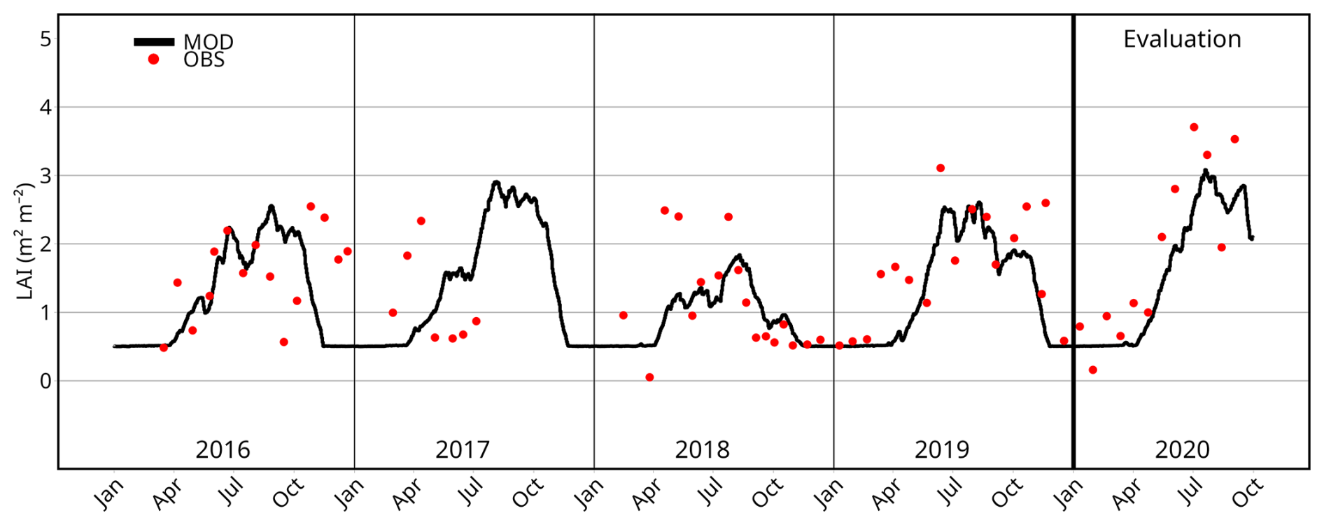
Figure 6 Daily evolution of the modelled LAI (black line) during the calibration (2016–2019) and evaluation (2020) periods compared to the estimated on-site LAI values (red dots), in m³ m⁻³.

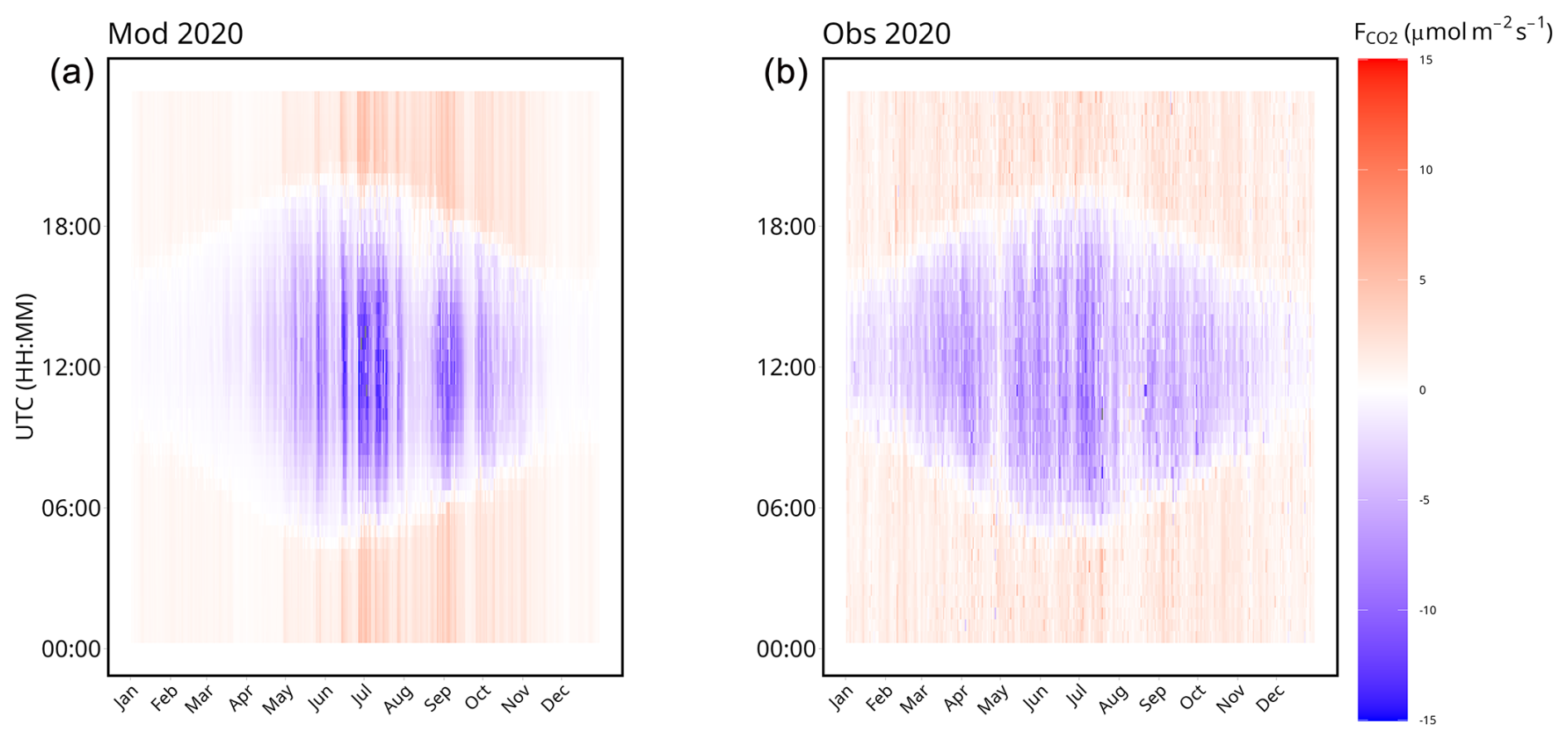
Figure 7 Monthly evolution of daily variation in modelled (a) and observed (b) CO₂ fluxes ($F_{{\mathrm{CO}}_{\mathrm{2}}}$) for the evaluation period 2020. The colour range varies from green for negative CO₂ fluxes (photosynthesis) to red for positive CO₂ fluxes (respiration).

5.3.2 Net CO₂ flux modelling

The monthly evolution of the net CO₂ flux diurnal cycle simulated and observed over the year 2020 is represented in Fig. 7. The model provides a good representation of the amplitude of the net CO₂ fluxes for the evaluation period. Both the annual cycle and the diurnal cycle are close to the observations. The model is able to capture the net CO₂ flux seasonal variations in response to variation in climatic forcing. In August and late April, both the model and the observations catch less photosynthesis due to a drier period of stress for the vegetation. Conversely, the model also reproduces periods in July when photosynthesis is enhanced. However, the model remains excessively responsive to meteorological fluctuations, particularly following precipitation events, when soil water content is high, leading to an overestimation of photosynthesis. This is illustrated after the rain of 13 June 2020, when the daily average (between 06:00 and 18:00 UTC) of the difference between the observation and the model is 3.35, 4.17, 2.93, and 2.42 $\mathrm{\mu }\mathrm{mol}{\mathrm{m}}^{-\mathrm{2}}{\mathrm{s}}^{-\mathrm{1}}$ for the 14th, 15th, 16th, and 17th, respectively, leading to an overestimation of the flux for the 4 d after the rain event. When this trend reverses, the difference between the observations and the model is then 0.89, −1.57, and −2.35 µmol m⁻² for the 18th, 19th, and 20th, respectively. Furthermore, outside the growing season, the photosynthesis simulated by the model is close to 0, whereas observations indicate that photosynthesis continues even during winter. This can be seen by taking the average over the meteorological winter period of the daily minimum $F_{{\mathrm{CO}}_{\mathrm{2}}}$. The observed value is 2.53 $\mathrm{\mu }\mathrm{mol}{\mathrm{m}}^{-\mathrm{2}}{\mathrm{s}}^{-\mathrm{1}}$, while the modelled value is only 0.40 $\mathrm{\mu }\mathrm{mol}{\mathrm{m}}^{-\mathrm{2}}{\mathrm{s}}^{-\mathrm{1}}$.

The diurnal cycle of the net CO₂ fluxes averaged monthly over the 5-year period is illustrated in Fig. 8. Similarly to what is shown in Fig. 7, outside the growth period (between November and March), the model does not simulate the diurnal CO₂ cycle, which is still noticeable in the observations and reflects weak but still active photosynthesis. However, the amplitude of the net CO₂ fluxes is on average quite well represented during the growing period, especially between June and October. During the day, the CO₂ fluxes are well represented, although the model tends to be overly responsive compared to the observations, resulting in a greater standard deviation for the modelling. The modelled respiration at night is in close agreement with the measurements, as can be seen between 20:00 and 06:00 UTC, and follows the annual variation well, being greater during the growing period and close to 0 outside the growing period.

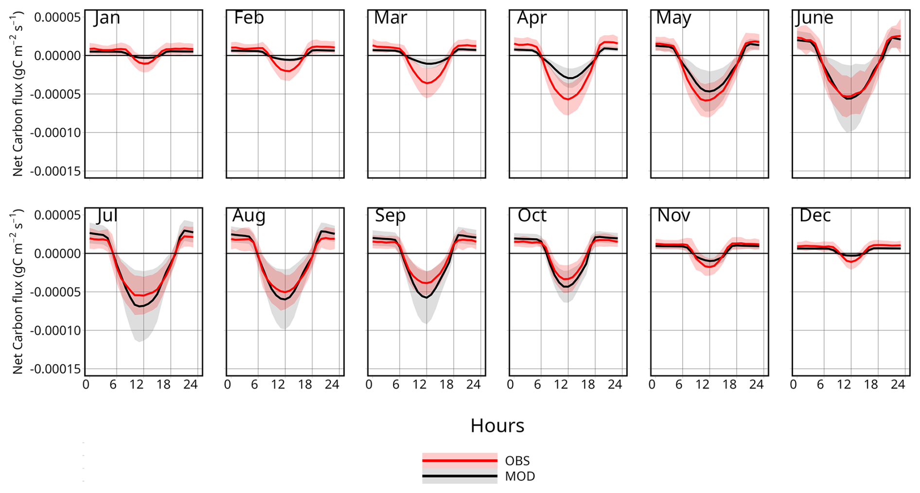
Figure 8 Comparison of the modelled (black line) and observed (red line) diurnal cycles of net CO₂ fluxes ($\mathrm{g}{\mathrm{s}}^{-\mathrm{1}}{\mathrm{m}}^{-\mathrm{2}}$) averaged monthly over the 5-year period. The transparent ranges indicate 1 standard deviation.

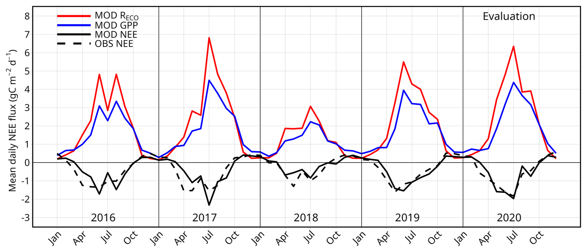
Figure 9 Comparison of the modelled (black line) and observed (dashed black line) monthly averaged daily NEE (in $\mathrm{g}\mathrm{C}{\mathrm{m}}^{-\mathrm{2}}{\mathrm{d}}^{-\mathrm{1}}$) for the period 2016–2020. For simulation only, the monthly averages of both daily ecosystem respiration (red line) and daily GPP (green) are also presented.

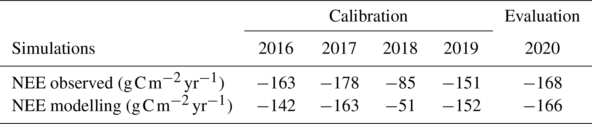
Table 3 Comparison of modelled and observed annual NEE in $\mathrm{g}\mathrm{C}{\mathrm{m}}^{-\mathrm{2}}{\mathrm{yr}}^{-\mathrm{1}}$ for each year from 2016 to 2020. By definition, a negative NEE corresponds to a quantity of carbon fixed by the green roof.

5.3.3 Net ecosystem exchanges

The net ecosystem exchange (NEE; see Sect. 3.3) quantifies the net sequestration of CO₂ if the NEE is negative or the net CO₂ emissions if the NEE is positive. Figure 9 represents the observed and modelled daily NEE averaged monthly for the 5 successive years from 2015 to 2020. The modelled NEE is in close agreement with the measurements for all years. It follows the observed annual variation, with a slightly positive NEE from October to March and negative NEE for the rest of the year. This means that the green roof acts as a net carbon emitter in autumn and winter but as a net carbon sink in spring and summer. The partitioning on the modelling between GPP and R_ECO in Fig. 9 demonstrates that both GPP and R_ECO follow similar inter-annual variations, being greater in summer than in winter. However, since no partitioning is available between GPP and R_ECO on observations during this study, it is not possible to confirm the accuracy of the model processes. At the annual scale (Table 3), the model shows that the green roof is a net carbon sink, in accordance with measurements, and quantifies the amount of carbon fixed by the green roof within the range of error of the measurement estimated at 16 $\mathrm{g}\mathrm{C}{\mathrm{m}}^{-\mathrm{2}}{\mathrm{yr}}^{-\mathrm{1}}$ fairly well. Indeed, the observed and modelled annual NEE for the evaluation year 2020 is −168 and −166 $\mathrm{g}\mathrm{C}{\mathrm{m}}^{-\mathrm{2}}{\mathrm{yr}}^{-\mathrm{1}}$, respectively. The model is also able to capture the inter-annual variations in NEE, which are partly governed by changes in weather conditions, especially in the year 2018, which stands out as a dry year compared with normal years and shows a lower annual NEE than the other years in both observations and the simulation (−85 and −51 $\mathrm{g}\mathrm{C}{\mathrm{m}}^{-\mathrm{2}}{\mathrm{yr}}^{-\mathrm{1}}$, respectively). Inversely, the wetter year 2017 presents an observed NEE of −178 $\mathrm{g}\mathrm{C}{\mathrm{m}}^{-\mathrm{2}}{\mathrm{yr}}^{-\mathrm{1}}$ that is substantially greater than for all other years. This is partly seen in the modelling results, where the NEE is high and reaches −163 $\mathrm{g}\mathrm{C}{\mathrm{m}}^{-\mathrm{2}}{\mathrm{yr}}^{-\mathrm{1}}$ in 2017, but it is in the same range than for the year 2020 (−166 $\mathrm{g}\mathrm{C}{\mathrm{m}}^{-\mathrm{2}}{\mathrm{yr}}^{-\mathrm{1}}$).

6 Discussion

The work presented in the previous section has enabled us to characterize, for the first time, the parameters of the photosynthesis and vegetation growth model for Sedum in a soil–vegetation–atmosphere transfer model. We now discuss in more detail the behaviour of the net CO₂ fluxes from green roofs in the TEB model and the perspectives that evolving vegetation opens up for the modelling of green roofs.

6.1 Sedum model response to micro-meteorological conditions

The calibration proposed in this study allows for the representation of Sedum behaviour when they do not use a CAM photosynthesis pathway. Here we investigate the response of the new Sedum parameterization to the environmental variables driving photosynthesis (soil temperature, water content, and radiation) compared to the standard C₃ and C₄ parameterizations. Figure 10 shows the response curves of GPP to the three environmental variables, T_s, PAR, and VWC, in each panel. For each response curve corresponding to one variable, the other environmental variables are fixed. For comparison, the observations are selected within the range of the most extreme values of the three curves (the dashed and dotted lines). The observed GPP displayed in the three figures is estimated from the observation of net CO₂ fluxes on the BER green roof site subtracted by the modelled R_ECO of the best simulation. All observations were conducted within the specified range of each figure, with variables influencing photosynthesis varying between the most and the least favourable values for photosynthesis. For the three curves, the Sedum parameterization performs better than the ISBA C₃ and ISBA C₄ parameterizations, with a significantly lower photosynthetic rate. The response to volumetric water content (Fig. 10a) demonstrates that the threshold values for the normalized water stress factor (F2_min and F2_max) and the weighted soil volumetric water content between 0–10 cm depth for soil respiration ($w_{{\mathrm{10}}_{\text{min}}}$ and $w_{{\mathrm{10}}_{\text{max}}}$) were appropriately selected. This is visible on the plateau reached at a VWC of 0.056 m³ m⁻³ under average micro-meteorological conditions (straight line), which correspond well with the observations. With regard to the photosynthetically active radiation (Fig. 10b), the Sedum parameterization models correctly represent the increase in GPP but also the threshold above which the GPP no longer increases with photosynthetically active radiation. This response is not noted with the ISBA C₃ and ISBA C₄ parameterizations. For the response to temperature (Fig. 10c), the range of temperatures observed does not allow determination of the maximum GPP achievable at higher temperatures, beyond which the GPP decreases with temperature.

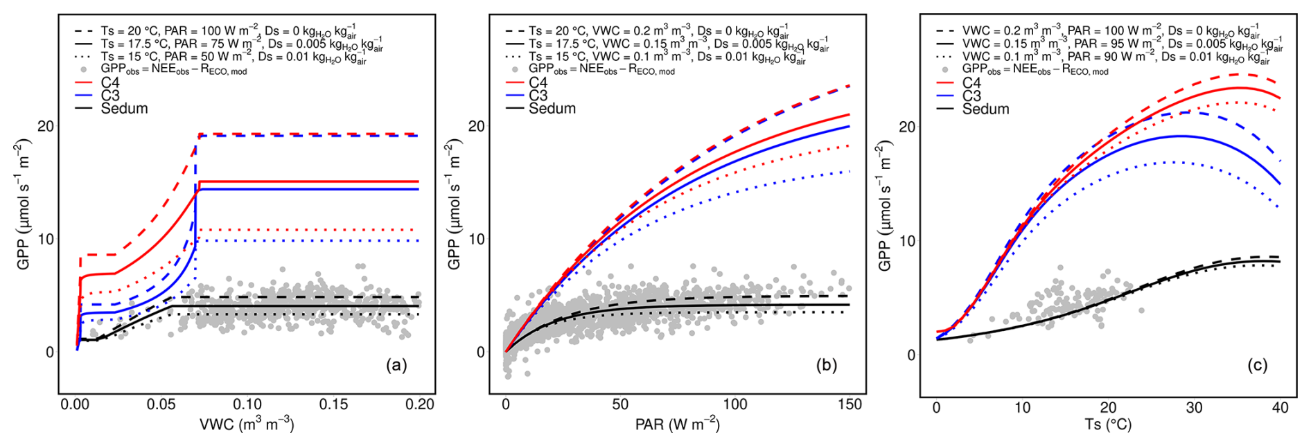
Figure 10 Evolution of the modelled (lines) GPP with (a) volumetric water content (VWC; m³ m⁻³), (b) photosynthetically active radiation (PAR; W m⁻²), and (c) temperature (T_s; °C), for the parameterizations of Sedum, ISBA C₃, and ISBA C₄ and the comparison against selected observations (dots).

6.2 Dynamic vegetation

The use of a vegetation growth model makes it possible to simulate the explicit evolution of LAI. LAI is a key parameter for vegetation, including green roofs, which drives and sizes physiological processes and water, energy, and gas exchanges. For the same micro-meteorological conditions, fluxes can vary considerably depending on LAI and its evolution over time. Therefore, LAI has a direct impact on the energy and water balance through the calculation of evapotranspiration and on the carbon balance through the calculation of GPP. However, quantifying LAI and its evolution over time accurately is a challenge, given that both can vary considerably over the course of a year and from one year to the next, depending on the variability of climatic conditions. At the present study site in particular, LAI varies between 0.05 and 3.71 m² m⁻², with significant inter-annual variations as well.

Most green roof models use LAI as an input prescribed variable. The first approach for short-term simulations of several days is to define a fixed LAI value for the duration of the simulation (e.g. Lazzarin et al., 2005) and compare simulations with different prescribed LAIs to find the best configuration and quantify the sensitivity of green roof performance to LAI variation, as done by Del Barrio (1998) and Sailor (2008). Another approach is to use on-site LAI measurement, as done in the works of Ouldboukhitine et al. (2011), with direct measurement of LAI or with indirect estimation methods, as in Lazzarin et al. (2005), where LAI is calculated with measurements of soil evapotranspiration. Zhou et al. (2018) show that taking into account the seasonal evolutive LAI during the simulation, rather than applying a fixed LAI, leads to a significantly more relevant energy balance, resulting in a better quantification of the reduction in building temperature and energy consumption, in particular for long-term simulations. With this aim, they use a model to represent vegetation seasonal changes based on temperature and fixed maximum and minimum LAI using a modified Dickinson semi-empirical equation. The work presented here includes more climatic and environmental factors that impact vegetation growth, namely the soil water content, atmospheric pressure, temperature, humidity, photoactive radiation, and CO₂ concentration. In this way, the model can represent and estimate the biomass accumulation or loss due to meteorological changes. In contrast to other works, it enables us to more accurately represent long-term changes in the performance of green roofs, in particular due to the development of vegetation.

7 Conclusions

A new parameterization for the net CO₂ flux calculation has been implemented in the TEB-GREENROOF model using the ISBA–A-gs photosynthesis model with a biomass module and an empirical parameterization of ecosystem respiration. The modelling was informed by observations on an extensive non-irrigated Sedum green roof located at BER Airport. The sensitivity analysis results showed that the main parameters driving CO₂ fluxes on the green roof are the mesophyll conductance at 25 °C ($g_{\text{mes}}^{*}\left(\mathrm{25}\right)$), the CO₂ compensation concentration at 25 °C (Γ(25)), and the maximum initial quantum use efficiency (ϵ₀), which needed to be calibrated more carefully. The results after calibration showed that the model performed well in reproducing the diurnal cycle during the growing period and its dependence on the variations in meteorological conditions and soil water conditions. Outside the growing period, the model struggled in simulating the weak photosynthesis process that seems to persist based on observations. Nonetheless, as CO₂ fluxes remain very low during this period, the impact on the overall quantification of carbon sequestration is limited, leading to a good estimation of the annual NEE and its inter-annual variations. This work also ultimately allowed us to characterize, for the first time, the photosynthesis and growth parameters appropriate for modelling Sedum with the ISBA soil vegetation atmosphere transfer model.

Future development will need to include comparison between the ecophysiological parameters calibrated here and on-site measurements of green roof plant photosynthesis parameters. To study the full carbon cycle of the green roof, the management and maintenance of green roofs need to be addressed, especially with respect to the biomass that can be removed by gardeners. Similarly, the carbon sequestered in the soil needs to be quantified with on-site sampling. On the modelling side, the growth module needs to be improved, and a soil organic carbon module needs to be added in order to be able to perform longer-term studies.

In addition to thermal and hydrological effects, the short-term carbon sequestration can now be added to impact studies in order to have a full picture of the impact of green roofs on the fluxes at city scale and under different climate events and conditions. However, the green roof effect should be looked at not only in terms of fluxes, but also with regard to other effects that cannot be modelled in models like SURFEX, such as the effect on individuals, and biodiversity should also be taken into account, thus requiring researchers to cross-reference the results of different approaches.

Appendix A

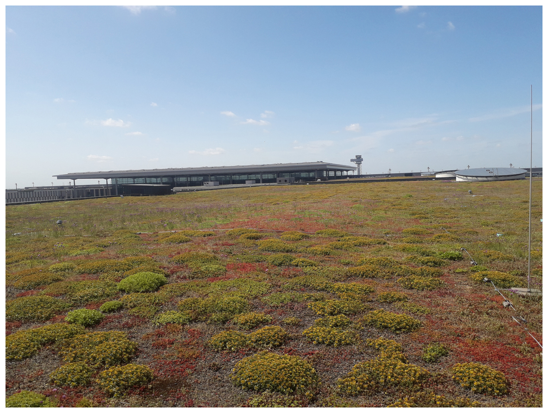
Figure A1 Photograph of the green roof experimental plot located on top of the car park of Berlin Brandenburg Airport (Germany).

Appendix B

A-gs equation

The following equations are used in ISBA–A-gs in SURFEX v9. The model uses an empirical light response function of net assimilation (A_n) to combine the effects of light and CO₂ as limiting factors. When light is not limiting, A_m is limited by a maximum photosynthetic rate A_m,max:

$$\begin{array}{}\text{(B1)}& A_m=A_{m,\text{max}}\left[\mathrm{1}-e^{-g_{\text{mes}}^{*}\frac{(C_{\mathrm{i}}-\mathrm{\Gamma })}{A_{m,\text{max}}}}\right],\end{array}$$

where C_i is the internal leaf CO₂ concentration in kg CO₂ per kg air. A_m,max is the maximum net CO₂ assimilation in $\mathrm{mg}{\mathrm{m}}^{-\mathrm{2}}{\mathrm{s}}^{-\mathrm{1}}$, $g_{\text{mes}}^{*}$ is the mesophyll conductance in m s⁻¹, and Γ is the CO₂ concentration compensation point in ppmv, defined according to the following equations:

$$\begin{array}{}\text{(B2)}& {\displaystyle }{A}_{m,\text{max}}\left(T_{\mathrm{s}}\right)={\displaystyle \frac{A_{m,\text{max}}\left(\mathrm{25}\right)\cdot Q_{\mathrm{10}}^{\frac{T_{\mathrm{s}}-\mathrm{25}}{\mathrm{10}}}}{(\mathrm{1}+e^{\mathrm{0.3}(T_{\mathrm{1}}-T_{\mathrm{s}})})\cdot (\mathrm{1}+e^{\mathrm{0.3}(T_{\mathrm{s}}-T_{\mathrm{2}})}),}}\text{(B3)}& {\displaystyle }{g}_{\text{mes}}^{*}\left(T_{\mathrm{s}}\right)={\displaystyle \frac{g_{\text{mes}}^{*}\left(\mathrm{25}\right)\cdot Q_{\mathrm{10}}^{\frac{T_{\mathrm{s}}-\mathrm{25}}{\mathrm{10}}}}{(\mathrm{1}+e^{\mathrm{0.3}(T_{\mathrm{1}}-T_{\mathrm{s}})})\cdot (\mathrm{1}+e^{\mathrm{0.3}(T_{\mathrm{s}}-T_{\mathrm{2}})}),}}\text{(B4)}& {\displaystyle }\mathrm{\Gamma }\left(T_{\mathrm{s}}\right)=\mathrm{\Gamma }\left(\mathrm{25}\right)\cdot Q_{\mathrm{10}}^{\frac{T_{\mathrm{s}}-\mathrm{25}}{\mathrm{10}}},\end{array}$$

where A_m,max(25) is the maximum net CO₂ assimilation at 25 °C in $\mathrm{mg}{\mathrm{m}}^{-\mathrm{2}}{\mathrm{s}}^{-\mathrm{1}}$, $g_{\text{mes}}^{*}\left(\mathrm{25}\right)$ is the mesophyll conductance at 25° in m s⁻¹, T_s is the leaf skin temperature in °C, and T₁ and T₂ are reference temperatures in °C.

The internal CO₂ concentration depends directly on the atmospheric CO₂ concentration (Eq. B5) and is controlled by the air humidity (Eq. B6):

$$\begin{array}{}\text{(B5)}& C_{\mathrm{i}}=f\cdot C_{\mathrm{s}}+(\mathrm{1}-f)\mathrm{\Gamma },\end{array}$$

where C_s is the atmospheric CO₂ concentration in kg CO₂ per kg air, and f is a coupling factor estimated via

$$\begin{array}{}\text{(B6)}& f=f_{\mathrm{0}}^{*}\cdot \left(\mathrm{1}-{\displaystyle \frac{D_{\mathrm{s}}}{D_{\text{max}}^{*}}}\right)+f_{\text{min}}\cdot \left({\displaystyle \frac{D_{\mathrm{s}}}{D_{\text{max}}^{*}}}\right),\end{array}$$

where $D_{\text{max}}^{*}$ is the maximum specific humidity deficit of the air tolerated by vegetation in kg H₂O per kg air, D_s is the leaf-to-air saturation deficit in kg H₂O per kg air, and $f_{\mathrm{0}}^{*}$ is the value of the f factor for D_s=0 g kg⁻¹ and f_min given by

$$\begin{array}{}\text{(B7)}& f_{\text{min}}={\displaystyle \frac{g_{\mathrm{c}}}{g_{\mathrm{c}}+g_{\text{mes}}^{*}}},\end{array}$$

where g_c is the cuticular conductance in m s⁻¹.

The CO₂ assimilation is then limited by the photosynthetically active radiation via

$$\begin{array}{}\text{(B8)}& A_{\mathrm{n}}=(A_m+R_{\mathrm{d}})\cdot (\mathrm{1}-e^{-\frac{\mathit{ϵ}*I_{\mathrm{a}}}{A_m+R_{\mathrm{d}}}})-R_{\mathrm{d}},\end{array}$$

where ϵ is the initial quantum use efficiency in ${\mathrm{kg}}_{{\mathrm{CO}}_{\mathrm{2}}}{\mathrm{J}}^{-\mathrm{1}}\mathrm{PAR}$, I_a is the photosynthetically active radiation, and R_d is the dark respiration ($R_{\mathrm{d}}=\frac{A_m}{\mathrm{9}}$). ϵ is estimated with the following (Eq. B9):

$$\begin{array}{}\text{(B9)}& \mathit{ϵ}={\mathit{ϵ}}_{\mathrm{0}}\cdot \left({\displaystyle \frac{C_{\mathrm{i}}-\mathrm{\Gamma }}{C_{\mathrm{i}}+\mathrm{2}\mathrm{\Gamma }}}\right),\end{array}$$

where ϵ₀ is the maximum quantum use efficiency in ${\mathrm{kg}}_{{\mathrm{CO}}_{\mathrm{2}}}{\mathrm{J}}^{-\mathrm{1}}\mathrm{PAR}$.

Plant respiration

Depending on whether the model is run with forced LAI or with interactive vegetation, plant respiration is estimated in two different ways. First, when the model is run with forced LAI, plant respiration R_leaf is calculated as

$$\begin{array}{}\text{(B10)}& R_{\text{leaf}}={\displaystyle \frac{A_m}{\mathrm{9}}}\cdot \text{LAI}.\end{array}$$

When the model is run with interactive vegetation, plant respiration is estimated, and an A term for the respiration of the above-ground stem biomass reservoir is added:

$$\begin{array}{}\text{(B11)}& R_{\text{leaf}}={\displaystyle \frac{A_m}{\mathrm{9}}}\cdot \text{LAI}+{\mathit{\eta }}_{\mathrm{R}}{B}_{\mathrm{s}}{Q}_{\mathrm{10}}^{T_{\mathrm{s}}-\mathrm{25}}\mathrm{\Delta }t,\end{array}$$

where B_s (expressed in kilograms of dry matter (DM) m⁻²) is the above-ground stem biomass reservoir, T_s is the leaf temperature in °C, η_R is a respiration rate fixed at 1 % d⁻¹ (s−1), and Q₁₀ = 2.0.

Appendix C

TEB-GREENROOF input parameters

Table C1 TEB-GREENROOF input parameters for roads, walls, and roofs.

Appendix D

Forced A-gs model

In order to reduce the cost of calculation, the A-gs component of the ISBA–A-gs model has been rewritten and implemented in R, allowing for the rapid execution of simulations without the necessity of computing each step individually. Indeed, the separated A-gs model is forced with computed ISBA–A-gs input from a reference TEB-GREENROOF simulation with forced LAI. This approach enabled the simulation to run every time step simultaneously; however, this approach removed the retroactive effect of the CO₂ fluxes. The LAI monthly evolution for the reference simulation was constructed using the monthly average of the spline interpolation of the punctually estimated values of LAI at the green roof case study site.

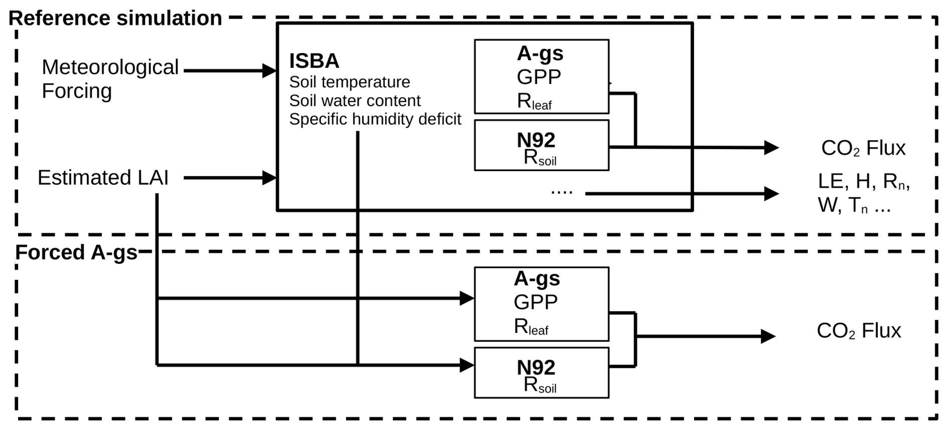
Figure D1 Description of the numerical setup implemented for running the A-gs photosynthesis model in a standalone configuration.

Appendix E

Pre-calibration

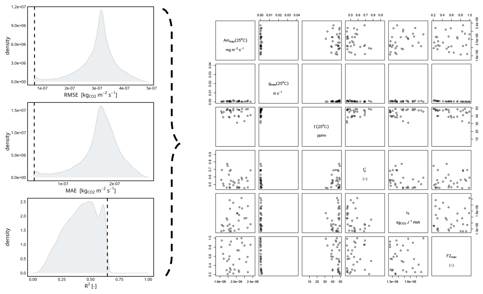
Before the calibration with the full TEB configuration, pre-calibration is done in order to reduce the plausible range of values and combinations of parameters for the calibration simulations. During the pre-calibration, the identified sensitive parameters ($g_{\text{mes}}^{*}\left(\mathrm{25}\right)$, Γ(25) ϵ₀, A_m,max(25), $f_{\mathrm{0}}^{*}$, and F2_max) are modified by conducting multiple simulations on the forced A-gs model, with the same parameter range and sampling method as those used in the sensitivity analysis but only on the sensitive parameters. A total of 50 000 simulations were conducted on the specified range of parameters. The intersection of the 0.1 % best simulations for the three scores, root-mean-square error (RMSE), mean absolute error (MAE), and coefficient of determination (r²), was retained and is displayed in Fig. E1. The results showed that for the 0.1 % intersection for the three scores, the average value of $g_{\text{mes}}^{*}\left(\mathrm{25}\right)$ for the simulations was 0.0019 m s⁻¹. Thus, it was decided to test for the two values 0.001 and 0.002 m s⁻¹. For $f_{\mathrm{0}}^{*}$, the average was 0.56, but since the lower range was at 0.45, the values selected were 0.45 and 0.55. For Γ(25), the average was 43.1 ppmv, and the standard deviation was 8.86 ppmv, but, like for $f_{\mathrm{0}}^{*}$, the values reached the upper range set at 49.5 ppmv, so the two values selected were set to 45 and 55 ppmv. For ϵ₀, A_m,max(25), and F2_max, there was no clearly highlighted values. Consequently, the pair of values defined for ϵ₀ and for A_m,max(25) was chosen based on the ISBA–A-gs C₃ and C₄ values. For F2_max, the values selected were 0.35 and 0.75.

Figure E1 Pre-calibration results. On the left is the distribution for RMSE, MAE, and r².