Interpolating turbulent heat fluxes missing from a prairie observation on the Tibetan Plateau using artificial intelligence models

This paper evaluates the performances of mean diurnal variation (MDV), nonlinear regression (NR), lookup tables (LUTs), support vector regression (SVR), k-nearest neighbors (KNNs), gradient boosting (XGBoost), long short-term memory (LSTM), gated recurrent units (GRUs), and the Transformer model with a deep self-attention mechanism to interpolate the turbulent heat fluxes missing from a prairie observation on the Tibetan Plateau. Results indicated that the Transformer model outperformed the other methods that were tested. To further enhance the interpolation accuracy, a combined model of Transformer and a convolutional neural network (CNN), termed Transformer_CNN, was proposed. Herein, while Transformer focused primarily on global attention, the convolution operations in the CNN provided the model with local attention. Experimental outcomes revealed that the interpolations from Transformer_CNN surpassed the traditional single artificial intelligence model approaches. The coefficient of determination (R²) reached 0.95 in the sensible heat flux test set and 0.90 in the latent heat flux test set, thereby confirming the applicability of the Transformer_CNN model for data interpolation of turbulent heat flux on the Tibetan Plateau. Ultimately, the turbulent heat flux observational database from 2007 to 2016 at the station was imputed using the Transformer_CNN model.

1 Introduction

Tibetan land surface processes play a significant role in influencing Asian weather and climate, primarily through the surface–atmosphere exchange of energy, momentum, and CO₂ across the atmospheric boundary layer (Zhang et al., 1996; Collatz et al., 2000; Defries et al., 2002; Chen et al., 2003, Gao et al., 2004, Jiao et al., 2023). Surface turbulent heat fluxes, including sensible and latent heat fluxes, are fundamental determinants of local microclimate formation and serve as crucial regulators of vegetation activity (Chapin et al., 2011). With global climate change, the ecosystems and water resources of the Tibetan Plateau have experienced significant impacts (Ren and Xu, 2016). Turbulent heat flux data provide key insights to assess these changes and devise countermeasures. Therefore, the long-term continuous observational data of land–atmosphere turbulent heat flux on the Tibetan Plateau have significant value for studying the region's weather and climate (Swinbank and W.C., 1951; Baotian et al., 1996; Zheng et al., 2000; Baldocchi, 2014; Yu et al., 2017).

As a direct observation technique for turbulent heat flux, the eddy covariance (EC) method stands as the primary observational means for an international flux network (FLUXNET) and a plethora of meteorological, ecological, and hydrological observation sites (Shaoying et al., 2020). Initially proposed by Swinbank (1951), EC directly measures the turbulent pulsations of various physical quantities based on micrometeorological principles. It calculates flux by evaluating the covariance produced by wind speed pulsations and physical quantity pulsations during atmospheric turbulent motion, thereby measuring heat, mass, and momentum exchanges between the land and the atmosphere. While this method does not rely on assumptions like the near-surface similarity theory, due to observational principles and instrument construction, a series of necessary corrections, quality controls, and quality assurances must be applied to raw data before obtaining final flux calculation results (Lee et al., 2004). Additionally, given the Tibetan Plateau's geographical location, high altitude, and harsh natural conditions, during continuous observations of material and energy exchanges between the land and atmosphere, data omissions account for 40 % to 60 % of the total number of data. This significant omission rate profoundly affects data integrity and accuracy (Falge et al., 2001; Lee et al., 2004), subsequently influencing their application in climate and weather models (Stull, 1988). Over the past 2 decades, local and international scientists have extensively researched the quality control and assurance of turbulent flux data, formulating standardized processing procedures (Papale et al., 2006; Mauder et al., 2008; Wang et al., 2009; Wutzler et al., 2018). However, discussions regarding the interpolation of missing flux data remain necessary (Foltynova et al., 2020). Rational interpolation methods can enhance the integrity of observational data series, facilitating a more accurate understanding of dynamic changing processes and laying the foundation for simulation experiments. In research on energy and material exchanges between terrestrial ecosystems and the atmosphere, the choice of interpolation method is paramount. Seasonal changes in ecological processes and soil moisture can influence measurements of turbulent exchanges (Reichstein et al., 2005). Therefore, selecting interpolation methods that capture such complexities is crucial.

So far, prior studies have developed dozens of interpolation methods, which can be mainly categorized into the following three types: (1) interpolation methods based on mean values, (2) nonlinear regression methods driven by environmental factors, and (3) interpolation methods based on machine learning algorithms (Falge et al., 2001; Hui et al., 2004; Ooba et al., 2006; Moffat et al., 2007; Soloway et al., 2017; Wang et al., 2020). A rational approach to imputing missing flux data serves as a crucial foundation for data integration among stations and flux observation networks and is a key factor in enhancing data comparability (Wang et al., 2009). However, the methods for imputing flux data across various flux observation networks have not been standardized. For instance, FLUXNET and the European flux network CarboEurope adopted marginal distribution sampling (MDS) from the mean value interpolation methods and successfully applied it to the FLUXNET2015 dataset (Papale et al., 2006; Soloway et al., 2017). Meanwhile, ChinaFLUX and the Japanese flux network opted for nonlinear regression methods to impute the net ecosystem exchange, while the sensible and latent heat fluxes were imputed using the day–night average transition method and the lookup table method (Li et al., 2008). The Australian national ecosystem research network OzFlux employed artificial neural network algorithms for interpolation (Beringer et al., 2017), while the US flux network AmeriFlux selected both MDS and artificial neural networks to impute missing flux data (Agarwal et al., 2014). The aforementioned studies suggest that machine learning algorithms have gradually been incorporated into the domain of missing flux data interpolation and have demonstrated promising performance (Moffat et al., 2007; Dengel et al., 2013; Knox et al., 2015; Beringer et al., 2017).

Machine learning technology, as a rapidly advancing supercomputing domain (Ortega et al., 2023), has already demonstrated its potential value in data interpolation across sectors such as transportation, healthcare, and sensor networks (Duan et al., 2014; Matusowsky et al., 2020; Gad et al., 2021). The variability in turbulent heat flux represents an extremely complex process. This suggests that simple linear models may not accurately capture the complex relationships between meteorological elements and turbulent heat flux. Consequently, in some instances, traditional statistical methods may fail to provide accurate predictions. Machine learning models can handle the complex nonlinear relationships between predictive variables, regardless of their interdependencies or correlations, and the expected outcomes. Compared to traditional machine learning techniques, the superiority of deep learning in heat flux data interpolation lies not only in its capacity to integrate more environmental driving variables that affect flux exchanges, but also in its more precise ability to handle nonlinear data patterns (Fawaz et al., 2019). This is attributed to deep learning's ability to learn complex data features through multilayer neural networks, thereby more precisely capturing intricate relationships inherent in the data. Over the past decade, deep learning has expanded from image- and text-processing domains to time series analysis. Specifically, recurrent neural networks (RNNs) and their variants, such as long short-term memory (LSTM) networks and gated recurrent units (GRUs), have been proven to excel in handling sequential data. They capture long-term dependencies and nonlinear patterns in the data, optimizing the accuracy of time series predictions. Furthermore, the Transformer architecture, with its attention mechanism, has offered a novel approach to processing time series data, showing superiority in time series simulations (Vaswani et al., 2017). Convolutional neural networks (CNNs), initially designed primarily for image recognition, have in recent years been applied successfully to the analysis and forecasting of time series data. Unlike traditional image processing, time series CNN models typically operate on one-dimensional data. CNNs capture local patterns and trends in time series data through local receptive fields and weight sharing. Local features and dependencies in time series, such as periodic patterns or break points, can be captured efficiently by convolutional layers. These attributes allow CNNs to outperform traditional methods and other deep-learning models in certain time series tasks, such as anomaly detection, pattern recognition, and forecasting. Concurrently, the multilayer convolutional structure enables the model to automatically extract multiscale features from the data. However, the practical application of deep learning in turbulent heat flux interpolation remains nascent, especially in the Tibetan Plateau region, with related studies still being sparse.

Unlike most prior studies, the present work attempted to evaluate the performances of various artificial intelligence models in interpolating the turbulent heat flux data for the Qomolangma Special atmospheric processes and environmental changes Monitoring Station (QOMS) site. In order to complete the interpolation of turbulent heat flux for this site spanning the years from 2007 to 2016 and make this dataset publicly accessible, the objectives of this study are to quantitatively compare the outcomes of different artificial intelligence models and propose a novel turbulent heat flux interpolation method based on deep learning.

2 Materials

2.1 Site

The data used in this study originate from the third Tibetan Plateau experiment at the QOMS station located at the bottom of the Rongbuk Valley to the north of Mount Everest (28.36° N, 86.95° E; 4298 m), as shown in Fig. 1 (adapted from Ma et al., 2020). The surface at the observation point is barren with relatively flat and open terrain and sparse and low vegetation. From the surface to the deeper soil layers, it mainly consists of sand and gravel. This observation station is influenced by local climate variations and weather processes as well as the regional circulations of the Himalayan range, such as valley winds. These local factors make it an ideal location for monitoring surface processes on the Tibetan Plateau.

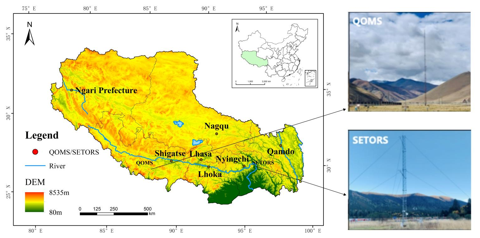
Figure 1 Geographical location and site images of the QOMS station. The map on the left provides a geographical overview of the Tibetan Plateau, while the site on the right is adapted from Ma et al. (2020). Publisher's remark: please note that the above figure contains disputed territories.

During the observation period, the average values for temperature, relative humidity, and annual precipitation were 4.16 °C, 43.47 %, and 289 mm, respectively. Wind speeds observed in winter are generally high, reaching up to 16 m s⁻¹, and are relatively lower in summer. At midday in summer, surface temperatures can rise to 60 °C. Correspondingly, consistent with the annual summer rainfall pattern, surface humidity peaks in summer.

2.2 Site data

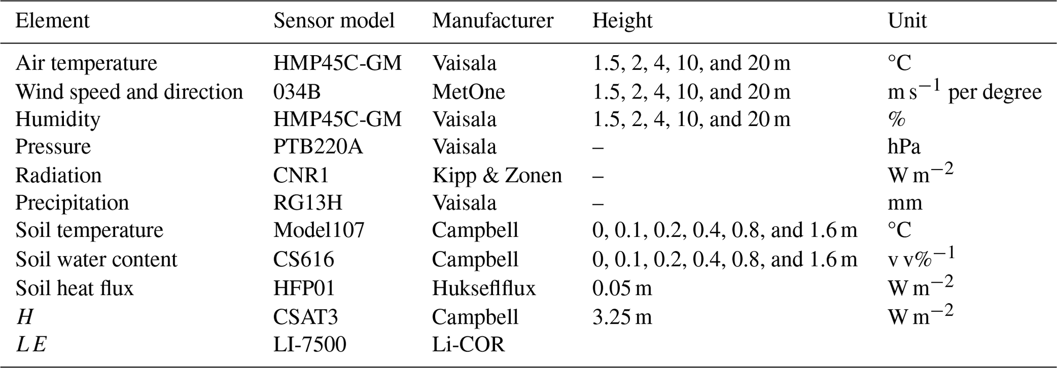
This study analyzes the observational data from the QOMS observation site from 1 January 2007 to 31 December 2016; the sampling frequency for all of the variables is hourly. Specific variables include sensible heat flux H, latent heat flux LE, soil heat flux SHF, air temperature at five levels Tair (1.5, 2, 4, 10, and 20 m), relative humidity at five levels RH (1.5, 2, 4, 10, and 20 m), wind speed at five levels WS (1.5, 2, 4, 10, and 20 m), wind direction at five levels WD (1.5, 2, 4, 10, and 20 m), downward shortwave radiation Rsd, upward shortwave radiation Rsu, downward longwave radiation Rld, upward longwave radiation Rlu, soil temperature at six levels T_soil (0, 0.1, 0.2, 0.4, 0.8, and 1.6 m), and soil volumetric water content at six levels SWC (0, 0.1, 0.2, 0.4, 0.8, and 1.6 m). The instruments used at the site are shown in Table 1.

Table 1 Summary of the meteorological and soil measurement instruments.

From 2007 to 2016, the missing rates for H and LE at the observation site (including missing and distorted data), denoted as gap_H and gap_LE, were 21.7 % and 21.4 %, respectively (Table 2).

Table 2 Missing rates for the sensible heat flux and latent heat flux.

2.3 Data preprocessing

To interpolate missing flux data using machine learning algorithms, it is essential to ensure the completeness of environmental driving variables (Wang et al., 2009). Therefore, during the data preprocessing phase, this study employed the k-nearest neighbor (KNN) interpolation method to address the missing data of environmental driving variables. The choice to set the number of neighbors to three is based on the consideration that a smaller number of neighbors can reduce computational complexity and enhance the efficiency of the interpolation process while maintaining accuracy. Additionally, “distance” was used as the weight calculation method to ensure that observations closer in distance receive higher weights (Friedman et al., 2009). This is given by Eq. (1):

$$\begin{array}{}\text{(1)}& \text{gap-filling value = }{\displaystyle \frac{{\sum }_{\mathrm{i}=\mathrm{1}}^{\mathrm{3}}\frac{y_i}{d_i}}{{\sum }_{\mathrm{i}=\mathrm{1}}^{\mathrm{3}}\frac{\mathrm{1}}{d_i}}},\end{array}$$

where y_i is the observation of the ith nearest neighbor and d_i is the distance between the missing value and the ith nearest neighbor. In this study, by setting weights equal to the distance parameter, KNN imputation (KNNImputer) is done using a weighted Euclidian distance formula. The numerator involves the weighted sum based on the observations and the reciprocal of the distances of the three nearest neighbors. The denominator is the sum of the reciprocals of the distances for these three nearest neighbors.

Subsequently, the fit_transform method (from the scikit-learn library in Python) is utilized to fit and transform the chosen data, facilitating the interpolation of missing values. Finally, we combined the estimated missing environmental driving variables with the actual observed environmental driving variables to create a complete and comprehensive dataset of environmental driving variables for subsequent analysis.

This KNN-based interpolation method has been demonstrated to be effective for datasets exhibiting similar patterns or local consistency (Little and Rubin, 2002). In other words, the KNN approach is applicable when the correlation length scale significantly exceeds the distance between missing and available data points. By considering the distances between observation points over time, this method can accurately estimate missing values, thereby enhancing the utility of the data for subsequent analyses.

Random forests assess the contribution of each variable to model predictive performance through importance ranking, with variables that contribute significantly to predictive performance receiving higher rankings. This importance is typically calculated by measuring the decrease in node impurity brought about by splits in each variable across all trees in the forest. Specifically, for each decision tree, the algorithm sums the impurity decrease from splitting in each variable and then averages this decrease over all of the trees to obtain an overall importance score for each variable. By sorting features based on their importance, random forests select the optimal feature combination, not only effectively reducing the dimensionality of input features but also aiding in the selection of variables within machine learning models. In this study, the number of trees for the random forest model was set to 159 based on 10-fold cross-validation and grid search algorithms, meaning that the model consists of 159 decision trees. Since bootstrapping (sampling with replacement) is used to generate random decision trees, not all samples participate in the tree generation process. The unused samples are referred to as out-of-bag (OOB) samples, which can be used to evaluate the accuracy of the trees. OOB scores provide an unbiased estimate of the model's generalization ability by effectively assessing the model's ability to predict unknown data. The higher the OOB score, the stronger the model's generalization capability (Wang et al., 2023).

Random forest analysis at the QOMS site on the Tibetan Plateau reveals that downward shortwave radiation has the greatest impact on sensible heat flux, while soil water content is most influential in latent heat flux, aligning closely with their respective roles in physical processes. The site is characterized by arid, barren, flat, and open terrain with sparse low vegetation primarily composed of sand and gravel from the surface to deeper soil layers. Such environmental conditions mean that less solar radiation is absorbed by plants for photosynthesis, allowing more shortwave radiation energy to reach the ground directly and thus increasing the surface heating. Moreover, the flat and open terrain, combined with sandy and gravelly textures, enables efficient absorption and reradiation of solar energy, significantly affecting the formation of sensible heat flux. In this arid and barren environment, soil water content plays a crucial role in regulating the surface energy balance, affecting predictions of latent heat flux significantly where even minimal variations can have substantial impacts under conditions of water scarcity. In conclusion, in subsequent analyses of turbulent heat flux, characteristics such as radiation, air temperature, soil temperature, and soil water content have high importance. However, whether to exclude some relatively less important features still requires further consideration and analysis.

The OOB scores in different input feature dimensions have been calculated, with variables input in order of importance, as shown in Fig. 2c. For the sensible heat flux, the OOB score is highest when considering the top 18 features ranked by importance. As shown in Fig. 2d, for the latent heat flux, the OOB score peaks when considering the top 16 features. Additional features added afterwards no longer impact the results. In other words, the environmental driving variables for sensible heat flux are the top 18 features, while those for latent heat flux are the top 16 features.

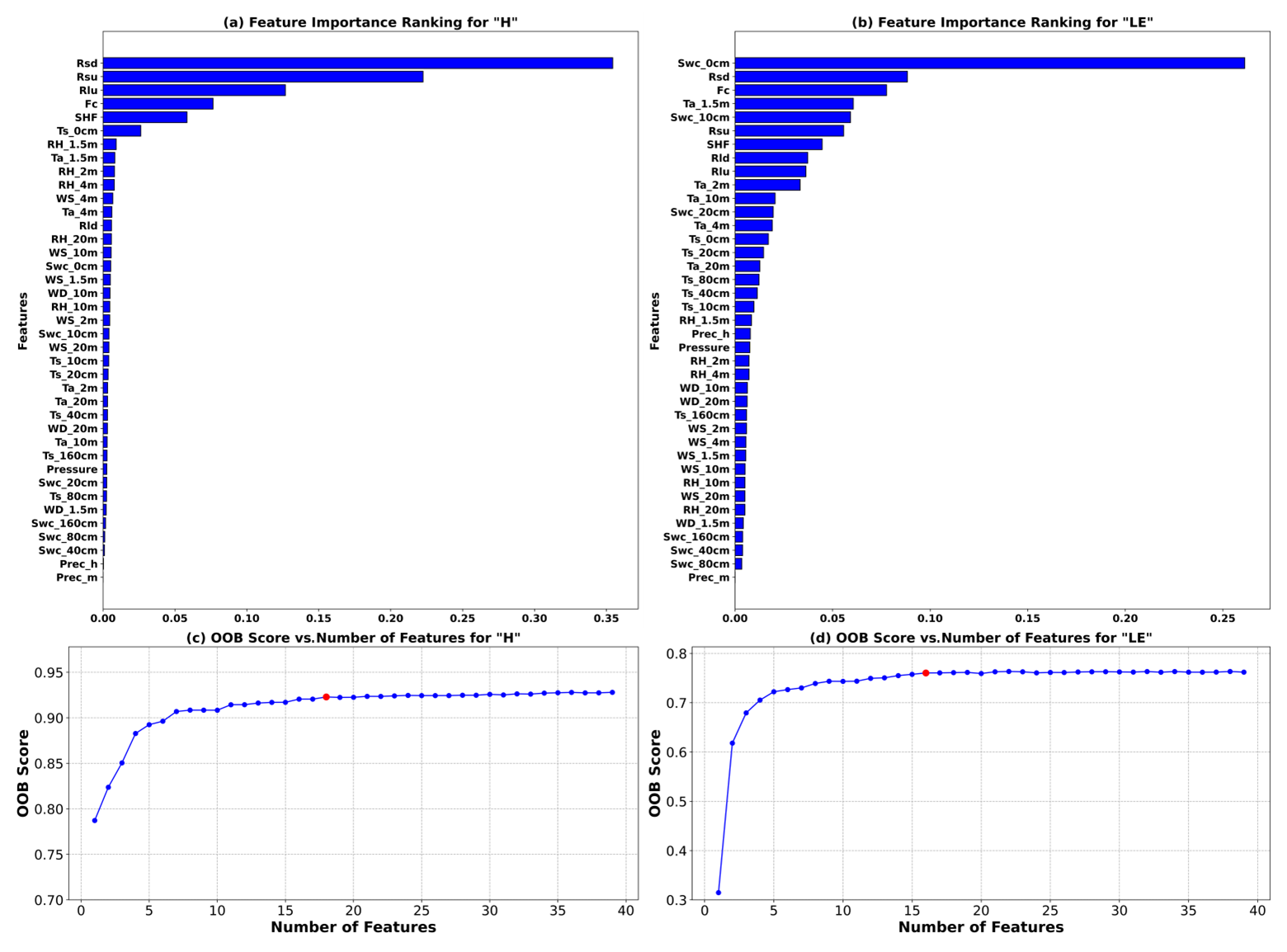
Figure 2 (a) Importance index for sensible heat flux (H). (b) Importance index for latent heat flux (LE). (c) OOB scores for different feature combinations of sensible heat flux based on random forest (the red dot indicates the maximum value). (d) OOB scores for different feature combinations of latent heat flux based on random forest (the red dot indicates the maximum value).

3 Experimental design and models

3.1 Experimental design

Here we present the experimental design and the different statistical and learning methods used in this study. The aim of this study is to use a decade's worth of observational data to fit missing values for sensible and latent heat fluxes. We explored the turbulence flux changes at the QOMS site from 2007 to 2016 and treated the missing parts of the turbulence flux in the dataset as quantitative prediction variables. The objective is to use other meteorological elements as environmental drivers to impute these missing data, forming a complete heat flux dataset.

In the research application of the model, it is crucial to correctly divide the training, validation, and test sets (Bishop and Nasrabadi, 2006; Friedman et al., 2009). The training set is used to train the model's parameters so that the model can learn and capture the underlying patterns and structures from the given data (Goodfellow et al., 2016a). The primary purposes of the validation set are model selection and hyperparameter tuning, enhancing the model's generalization capability (Cawley and Talbot, 2010). The test set offers a completely independent evaluation method to more accurately assess the model's performance on unseen data (Arlot and Celisse, 2010). This dataset has never been used in the training or validation processes, so it can serve as an unbiased estimate of the model's performance in practical applications (Kohavi, 1995). This study utilizes 10 years of data and employs a rolling forecasting approach for training and testing the model. Specifically, each year is selected sequentially as the test set, with the remaining 9 years used for training. For instance, the data from 2007 are initially used as the test set, while the data from the other years serve as the training set. This process is then repeated with 2008 as the test year, and so on. Notably, due to significant missing turbulence heat flux data in 2012, this paper will primarily present the data interpolation for that year, while the data handling for the other years is detailed in the Supplement. According to the research objectives and the length of the interpolated dataset, all samples are divided into three groups: a training set (2007–2011 and 2013–2016), with 10 % randomly extracted as the validation set, and the test set (2012). In total, there are 87 673 samples, with 80 % used for training, 10 % for validation, and the remaining 10 % for testing. Traditional statistical methods do not involve the division into training, validation, and test sets. To facilitate comparison in this study, we designate the data from 2012 as the test set and apply the traditional statistical methods for data interpolation. The data from the remaining years serve as the training set for our proposed method.

This design plan fully considers the complexity and diversity of time series analysis while ensuring the rigor of model validation and testing. In this way, it provides an accurate and reliable means of predicting soil turbulence heat flux.

3.2 Traditional statistical methods

Current techniques used for imputing missing data in turbulent heat flux include linear interpolation (Alavi et al., 2006), variable relationships (Soloway et al., 2017), mean diurnal variation (MDV) (Falge et al., 2001), nonlinear regression (NR) (Chen et al., 2012), and lookup tables (LUTs) (Falge et al., 2001). Linear interpolation is suitable only for small gaps (one to three consecutive missing data points), but on the Tibetan Plateau turbulent heat flux often exhibits prolonged periods of missing observations, rendering linear interpolation unreliable. Variable relationships utilize linear relationships between meteorological variables for mutual interpolation; however, due to the strong nonlinear relationships between turbulent heat flux and environmental driving factors, the mere method of variable relationships struggles to accurately capture the changes in turbulent heat flux. Additionally, the variable relationships vary across different sites on the vast and geographically diverse Tibetan Plateau. The daily variation method involves establishing a time window, typically between 4 and 15 d, with 7 and 14 d being the most common selections. The time window used in this study is 14 d. Within this window, averages of observations at the same time are computed to obtain a set of daily variation data, and missing data within these averages are imputed using linear interpolation and filled with corresponding daily variation data for the respective times. Nonlinear regression is based on an understanding of the main factors controlling the flux, thereby effectively capturing the impact of major environmental element changes on the flux, allowing for more accurate data interpolation. The lookup table method is based on creating a data retrieval table from valid data, searching for valid data under similar environmental conditions according to major environmental factors, and averaging the found data to impute missing data. Given the harsh geographical conditions of the Tibetan Plateau, we employ the daily variation method, nonlinear regression, and lookup tables at the QOMS site to impute data, exploring the gap between these methods and machine learning approaches.

3.3 Traditional machine learning methods

The Support Vector Machine (SVM) is versatile and can be applied not only as a linear classifier, but also for nonlinear classification through the use of kernel functions. Moreover, beyond its capability for classification, the SVM can be adapted for regression tasks – known as support vector regression (SVR). This approach aims to find an optimal hyperplane in a high-dimensional kernel space that best fits the data points, thereby ensuring optimal regression performance. This versatility allows SVR to address both classification and regression problems effectively (Cortes and Vapnik, 1995). XGBoost is a decision-tree-based gradient boosting algorithm that enhances the model's performance by progressively adding new trees and adjusting the errors of previous trees. It has been proven to perform excellently in various competitions and practical applications (Chen et al., 2016). The KNN algorithm is an instance-based learning method. It classifies or predicts by calculating the distance between the input data point and the data points in the training dataset, selecting the nearest K points and voting based on their labels (Cover and Hart, 1967). Each algorithm has its unique principle, offering multiple choices for addressing the problem of turbulent heat flux interpolation.

3.4 Recurrent neural network

RNNs are a class of deep-learning models designed for processing sequential data (Goodfellow et al., 2016a). The core idea is to share weights between the hidden layers of the network to capture temporal dependencies within sequences. However, standard RNNs suffer from issues of vanishing and exploding gradients, which limit their ability to capture long-term dependencies. LSTM networks address this problem by introducing special units with three gate structures, allowing the network to learn and remember long-term dependencies within sequences (Hochreiter and Schmidhuber, 1997). GRUs are variants of LSTM that improve computational efficiency by simplifying the gate structure and reducing the number of parameters while retaining the ability to capture long-term dependencies (Cho et al., 2014). These recurrent neural network architectures have achieved significant success in many sequence modeling and prediction tasks.

3.5 Transformer

The Transformer model is a deep-learning architecture that is widely used in natural language processing and other sequence-to-sequence tasks (Vaswani et al., 2017). It mainly consists of two parts: an encoder and a decoder. Transformer captures long-distance dependencies in sequences through the self-attention mechanism. Self-attention allows the model to consider other positions in the input sequence simultaneously in all positions, which, unlike traditional RNNs and LSTM networks, eliminates the need for sequential computation, thereby greatly enhancing parallel computation capabilities. Following each self-attention layer is a feed-forward neural network accompanied by layer normalization, which contributes to training stability and convergence. Transformer exhibits outstanding performance in data fitting and prediction (Li et al., 2019). Its ability in parallel computation allows it to process large datasets more quickly. The self-attention mechanism ensures that the model can capture complex dependencies, surpassing previous methods in many tasks (Wu et al., 2020).

3.6 Transformer_CNN

To address the high complexity of data from the Tibetan Plateau, a deep neural network model based on the PyTorch framework was adopted in this study, as illustrated in Fig. 3. At the initialization of the model (feed-forward), a layer normalization component was introduced with the aim of normalizing the input in the embedding dimension, thereby enhancing the stability and convergence rate of network training. Subsequently, a feed-forward neural network comprising three fully connected layers was defined, incorporating a rectified linear unit (ReLU) activation function to capture nonlinear features (please refer to the Supplement). This paper considers employing kernels of sizes 3, 5, and 7 to capture multiscale features. In the simulation of turbulent heat flux, turbulence phenomena display distinct characteristics at various spatial scales. Smaller kernels (such as 3) can capture more localized features, while larger kernels (such as 5 and 7) are able to cover a wider area, capturing more global features. This combination enables the model to concurrently learn features across different scales, thereby enhancing the model's understanding and predictive capacity regarding changes in turbulent heat flux. Following this, another one-dimensional convolutional layer was defined to integrate the outputs from the three previous convolutional layers, forming a comprehensive feature representation.

Figure 3 The model framework and network structure of Transformer_CNN.

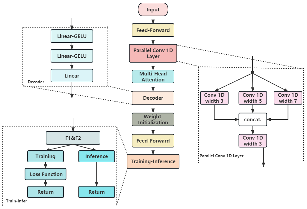
The multi-head self-attention mechanism was realized through the multi-head attention component, which boasts four attention heads capable of capturing long-distance dependencies within the input sequence. The decoder section of the model is responsible for mapping the encoded features to the target space. The initialization of weights and biases is designed to ensure the stability and efficiency of the model training process. Specifically, we adopted a variant of the HE15 initialization method (He et al., 2015), a scientific approach to weight initialization that is frequently employed in deep-learning models to improve convergence speed and stability during training. The core idea of HE15 initialization is to adjust the initial standard deviation of weights based on the number of nodes in the previous layer (i.e., fan_in). This initialization method is particularly crucial for the training of deep neural networks as it helps prevent issues of vanishing or exploding gradients, which often occur when traditional random weight initialization methods are used.

The forward-propagation process involves invoking the feed-forward function twice during each training iteration, resulting in two different outputs due to the stochastic nature of dropout layers. These outputs are referred to as two data “views”: F1 (primary view) and F2 (contrast view). Despite the presence of dropout, the two views might still differ. The loss function employed is the smooth L1 loss, which is comprised of three parts: the loss between F1 and the true value, the loss between F2 and the true value, and the distance between F1 and F2, which serves as a regularization term multiplied by 0.1. During model inference, the final prediction is derived from the average of F1 and F2 (Chen et al., 2020).

The Transformer_CNN model is a novel deep-learning framework specifically designed to address the complex physical phenomena of turbulent heat flux or similar challenges. It integrates the features of CNNs and Transformer, aiming to capture the intricate relationships of temporal dimensions. In this model, the CNN, through its convolutional layers, manages to capture the evident seasonal and cyclical variations in turbulent heat fluxes. By identifying these local patterns, it discerns the daily, monthly, and seasonal variations in turbulent fluxes, thereby having an edge in capturing intricate patterns within the data (Krizhevsky et al., 2012). Secondly, predicting turbulent heat fluxes encompasses intricate physical processes and multiscale interactions. The prowess of the Transformer model in capturing long-distance dependencies (Vaswani et al., 2017), combined with the CNN's local feature extraction capability, facilitates a superior grasp of the interactions between wind speed, temperature, and radiation with respect to turbulent heat fluxes, thereby enhancing the model's versatility and diversity. Moreover, the efficiency of convolutional operations might contribute to elevating the speed and efficiency of model training (Goodfellow et al., 2016b). By employing a hybrid model of the CNN and Transformer, both local and global features can be captured concurrently, thereby manifesting an adaptive advantage in data fitting for turbulent heat fluxes (Bello et al., 2019).

3.7 Statistical analysis

In this study, traditional statistical analysis indices were used to evaluate the accuracy of various models. The comparison statistics were calculated as follows.

Root mean square error (RMSE): RMSE represents the square root of the mean of the squared errors, which is the average of the differences between the simulated and observed values. The lower the RMSE value, the better the model's fit. The relationship between them can be expressed as Eq. (2):

$$\begin{array}{}\text{(2)}& \mathrm{RMSE}=\sqrt{{\displaystyle \frac{\mathrm{1}}{\mathrm{n}}}{\sum }_{\mathrm{i}=\mathrm{1}}^{\mathrm{n}}({\mathrm{y}}_i-{\widehat{y}}_i{)}^{\mathrm{2}}}.\end{array}$$

Mean absolute error (MAE): MAE calculates the average of the absolute differences between the observed and predicted values. A lower MAE value indicates a better fit of the model. The relationship between them can be expressed as Eq. (3):

$$\begin{array}{}\text{(3)}& \mathrm{MAE}={\displaystyle \frac{\mathrm{1}}{n}}{\sum }_{i=\mathrm{1}}^n\mathrm{|}{\mathrm{y}}_i-{\widehat{y}}_i\mathrm{|}.\end{array}$$

Coefficient of determination (R²): R² measures the proportion of the variance in the dependent variable that is predictable from the independent variables. This metric indicates how close the data are to the fitted regression line. The closer R² is to 1, the more effectively the model explains the data's variability. The relationship between them can be expressed as Eq. (4):

$$\begin{array}{}\text{(4)}& R^{\mathrm{2}}=\mathrm{1}-{\displaystyle \frac{{\sum }_{i=\mathrm{1}}^n(y_i-{\widehat{y}}_i{)}^{\mathrm{2}}}{{\sum }_{i=\mathrm{1}}^n(y_i-{\stackrel{\mathrm{‾}}{y}}_i{)}^{\mathrm{2}}}},\end{array}$$

where y_i represents the model-simulated value, $\widehat{y}$ denotes the observed value, and $\stackrel{\mathrm{‾}}{y}$ signifies the mean of the observed values. The subscript i represents the serial number of samples, and N represents the total number of samples.

3.8 Hyperparameter optimization

In this study, we employed a standardized hyperparameter optimization method. The batch size was set to 32 to control the number of samples used for each parameter update. The learning rate and weight decay parameters were gradually adjusted during training to optimize model performance. The initial learning rate was set to 0.0005 and halved every six epochs, with the weight decay parameter set to 0.01. The training was conducted over 100 epochs, with multiple iterations for model training and validation. During each iteration, we recorded the training loss and validation loss, using mean square error loss (MSELoss) and smooth L1 loss (SmoothL1Loss) to calculate the loss. Gradient clipping (with a maximum norm of 10) was applied to ensure training stability. Specifically, we updated model parameters using the training set and evaluated model performance on the validation set. The primary evaluation metric was the R-squared (R²) score. The hyperparameter optimization followed these steps:

• a.

  Initial training – the model was trained with the initial hyperparameter settings and evaluated on the validation set, recording the initial R² score on the validation set.

• b.

  Learning rate adjustment – after every six training epochs, the R² score of the validation set was checked. If the score improved, the current model parameter configuration was saved. Otherwise, the learning rate was halved, and training continued.

• c.

  Weight decay and batch size optimization – throughout the training process, the weight decay and batch size were kept constant to ensure training stability and convergence.

• d.

  Saving the best model – at the end of each training epoch, the R² score in the validation set was evaluated. If the current score was better than the previous best score, the current model parameter configuration was saved.

4 Results

The performances of the nine models (MDV, NR, LUT, SVR, KNN, XGBoost, LSTM, GRUs, and Transformer) were assessed by calculating the RMSE and MAE values between the predicted and actual values for both the sensible and latent heat fluxes. These evaluations are presented in Table 3, encompassing the training, validation, and test sets, with the best results highlighted in bold. The results are clear: whether for H or LE, traditional statistical methods are comprehensively outperformed by machine learning algorithms. Of the three traditional machine learning methods, the SVR model demonstrated superior performance in simulating the sensible heat flux, whereas XGBoost excelled in simulating the latent heat flux. Surprisingly, both RNN models exhibited sub-par performance in the task of simulating turbulent fluxes. Two predominant factors might account for these observations. One pertains to the challenges of gradient vanishing and explosion. Although LSTM models and GRUs alleviate the issues of gradient vanishing and explosion through gating mechanisms, these problems can still affect model performance when dealing with particularly long sequences. The second factor concerns the nuances of hyperparameter optimization in RNN models. Choosing the right set of hyperparameters, which are particularly numerous in RNNs, is crucial to achieving optimal model performance. Fortunately, the Transformer model showed exceptional prowess in the task of simulating turbulent fluxes. In almost all of the simulations, the Transformer model achieved the best performance, boasting the smallest RMSE and MAE in the test set. As a result, the Transformer model architecture was integrated into the neural network framework, and by further incorporating convolutional layers and multi-head attention mechanisms, the Transformer_CNN model was proposed, which was found to be superior in simulating turbulent fluxes.

Table 3 Model performance evaluation (RMSE and MAE) for MDV, NR, LUT, SVR, KNN, XGBoost, LSTM, GTU, and Transformer. Bold values highlight the best performance.

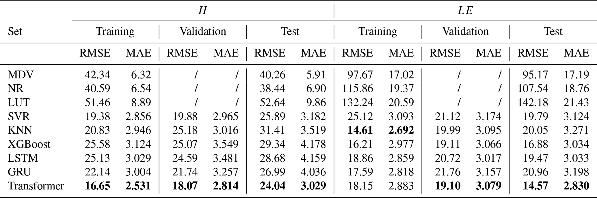
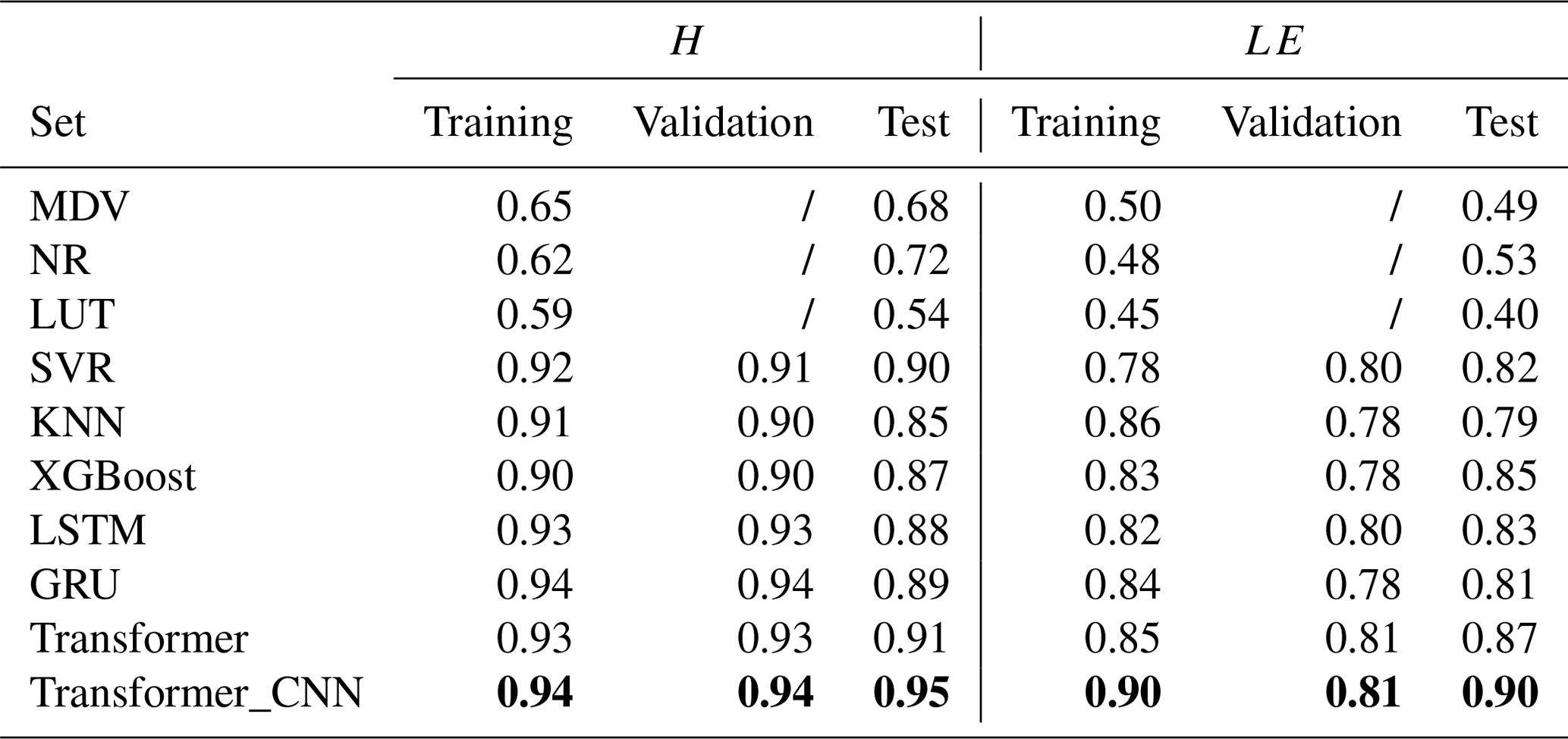
Table 4 juxtaposes the results of Transformer_CNN with various artificial intelligence models, illustrating the predictive outcomes in terms of R². Evidently, Transformer_CNN possesses a distinct advantage in long-term predictions. The performance of the Transformer_CNN model in data fitting surpassed that of the conventional Transformer model. The incorporation of the CNN enhanced the model's ability to extract local features (Lecun et al., 1998). In summary, the Transformer_CNN model, by amalgamating Transformer's global dependency capture capability with the CNN's local feature extraction prowess, offers a richer and more flexible model representation, thereby exhibiting superior performance in data fitting.

Table 4 Comparison of the coefficient of determination (R²) predicted by multiple models (MDV, NR, LUT, SVR, KNN, XGBoost, LSTM, GTU, Transformer, and Transformer_CNN). Bold values highlight the best performance.

To more comprehensively and intuitively describe Transformer_CNN, Fig. 4 displays a scatterplot of predicted values against actual values. The black dashed line represents the diagonal (1:1 line). The red line denotes the fitted regression line between the actual and estimated values. The color bar represents the density of the data points. Areas with redder hues correspond to regions of higher data density. The distance between the data points and the diagonal line indicates prediction errors. The results suggest that the majority of the turbulent heat flux values are centered around 0. Owing to the large volume of low-value data, the model is adept at capturing the characteristics of environmental driving forces when observed values are near 0, thereby achieving more accurate predictions. As the observed values increase, the prediction error of the model gradually amplifies. Furthermore, it was observed that, when the turbulent heat flux is substantial, the predicted values typically fall below the observed values. This phenomenon is more pronounced in the fitting of LE.

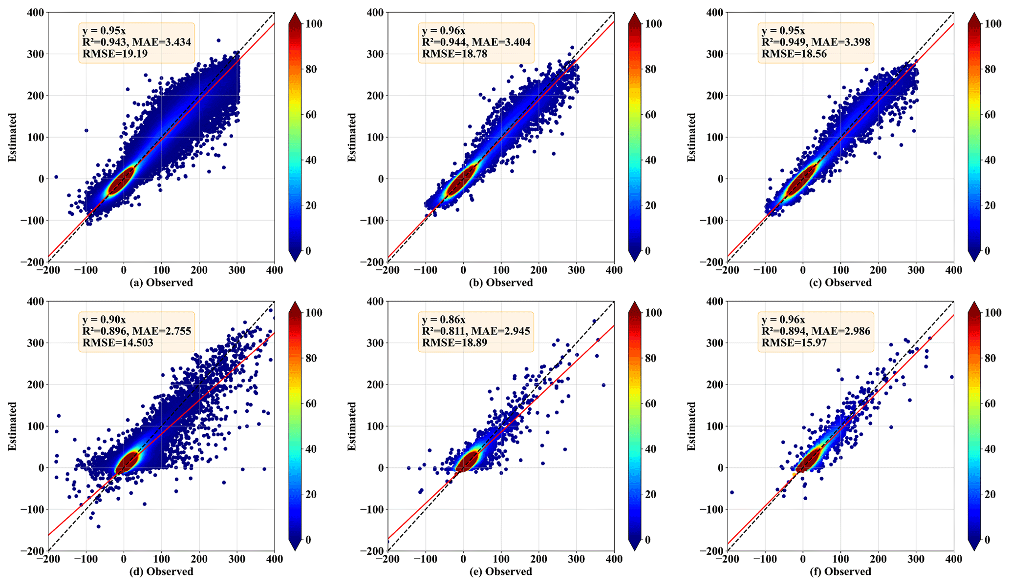
Figure 4 Scatter density plots of observed and Transformer_CNN-estimated sensible heat flux (H, W m⁻²) and latent heat flux (LE, W m⁻²) for the test set (2012), where panels (a) and (d) correspond to the training dataset, panels (b) and (e) to the validation dataset, and panels (c) and (f) to the test dataset. Panels (a), (b), and (c) show estimates for H, while panels (d), (e), and (f) show estimates for LE. The black dashed line represents the diagonal (1:1 line), and the red line denotes the fitted regression line between the actual and estimated values. The color bar represents the density of the data points, with redder hues indicating regions of higher data density.

To better display the predictions of the Transformer_CNN model, Fig. 5a and b show the monthly average diurnal variation curves for H and LE in the test set. The red line represents the observed values, while the blue and green lines represent the predictions of the Transformer and Transformer_CNN models.

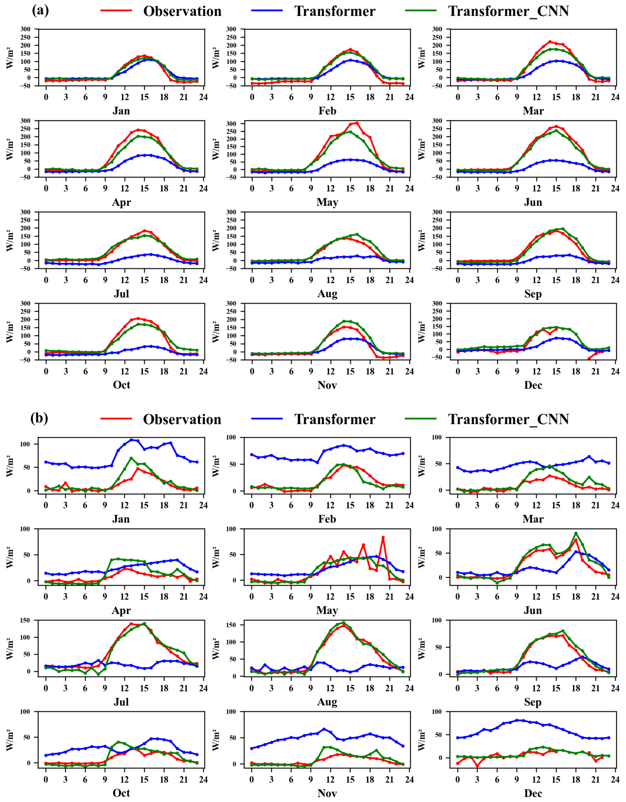
Figure 5 Monthly average diurnal variation curves of observed, Transformer-estimated, and Transformer_CNN-estimated sensible heat flux (H, W m⁻²) and latent heat flux (LE, W m⁻²) in the 2012 test dataset, where the red line represents the observed values, the blue line represents the Transformer estimates, and the green line represents the Transformer_CNN estimates (x axis in hours). Specifically, panel (a) represents H and panel (b) represents LE.

In the prediction of sensible heat flux, both the Transformer and Transformer_CNN models perform excellently for hours 0–9 and 19–23, where their predicted values closely align with the observed values. However, between 9 and 19 h, as the solar radiation intensity increases and the sensible heat flux grows rapidly, the Transformer model struggles to capture this escalating trend, resulting in a notable underestimation. The Transformer_CNN model, having incorporated convolutional layers, is better equipped to recognize periodic data changes and the impacts of environmental drivers on sensible heat, substantially rectifying the underestimation issues observed in high values.

In the latent heat flux prediction, the performance superiority of the Transformer_CNN model is even more pronounced. While the Transformer model exhibits significant overestimations during low-value periods and struggles to capture high values, the Transformer_CNN model's predictions largely coincide with observed values, significantly reducing the prediction errors exhibited by the Transformer model. Not only does it excel during the low-value periods of LE in January–March and October–December, it also accurately predicts the pronounced increase in LE in July–September. The experiments demonstrate that the Transformer_CNN model is well suited to serving as an artificial intelligence model for imputing turbulent heat fluxes.

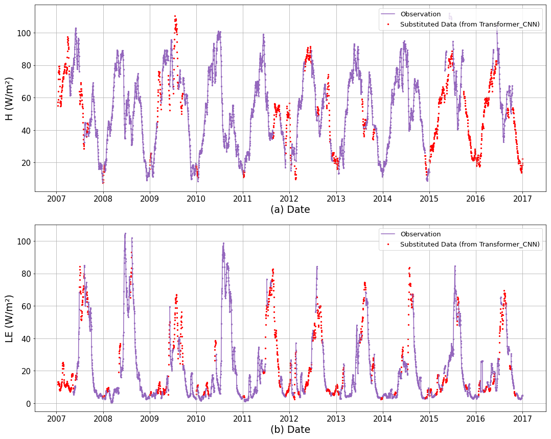
Figure 6 Observed values and Transformer_CNN-estimated values for the variation curves from 2007 to 2016 are presented. Specifically, panel (a) depicts H (W m⁻²), panel (b) illustrates LE (W m⁻²), the purple points represent the observed values, and the red points represent the imputed values generated by the Transformer_CNN model.

Based on the research presented earlier, it was determined that the Transformer_CNN model can serve as an artificial intelligence model for imputing turbulent heat fluxes. To delve deeper into the variation of turbulent heat fluxes at the QOMS site, the model was employed to impute data from 2007 to 2016 for the QOMS site, with the results shown in Fig. 6. The variation in sensible heat flux, as depicted in Fig. 6a, indicates that, prior to the monsoon season, the sensible heat flux is the primary consumer of the available energy at Earth's surface. With the onset of the summer monsoon, the diurnal variation of sensible heat flux significantly decreases, equating to the latent heat flux. In other words, during the pre-monsoon period, the exchange of sensible heat flux dominates. Influenced by the interaction of midlatitude westerlies and the summer monsoon, the summer sensible heat flux is significantly lower than that of spring. In contrast to the bimodal seasonal variation of sensible heat flux, the seasonal variation of latent heat flux exhibits a single peak pattern. That is, during the pre-monsoon period, the latent heat flux is small, but with the outbreak of the monsoon it rapidly increases due to frequent precipitation and the moistening of the surface soil. Subsequently, the latent heat flux gradually increases, equating to the sensible heat flux during the summer monsoon period. A comparison of the seasonal variations of the sensible heat flux (Fig. 6a) and the latent heat flux (Fig. 6b) suggests that, during the Asian summer monsoon season, the impacts of latent and sensible heat fluxes at the QOMS site are comparable. During the non-monsoon season in Asia, the site's sensible heat flux has a greater impact.

Table 5 Comparison of RMSE, MAE, and R² for the interpolated H and LE at the QOMS and SETORS stations for 2012, using three methods (Transformer with basic meteorological inputs, Transformer_CNN with basic meteorological inputs, and Transformer_CNN with the total meteorological inputs).

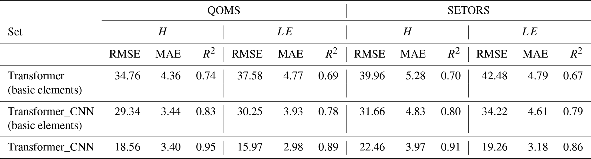
It is well known that many stations on the Tibetan Plateau cannot fully measure the 39 variables listed in the importance ranking of Fig. 2. To better validate the model's applicability on the Tibetan Plateau, Table 5 below presents the interpolation results using Transformer_CNN at the QOMS and Southeast Tibet Observation and Research Station for the Alpine Environment (SETORS) sites (29.77° N, 94.73° E; 3327 m), with the year 2012 as the test set. The model employs basic meteorological elements, including single-layer air temperature, pressure, single-layer air humidity, single-layer wind speed, single-layer wind direction, site hourly average precipitation, ground net radiation, single-layer soil temperature, and single-layer soil moisture content. As shown in Table 5, the interpolation performance using basic meteorological elements is significantly lower than that using all of the variables, but it still presents a generally good result. When employing basic meteorological elements for data interpolation, the Transformer_CNN model consistently outperforms the single Transformer model. This superiority is evident at both the QOMS and SETORS sites. In particular, at the SETORS site, the better interpolation performance further validates the high applicability of the Transformer_CNN model on the Tibetan Plateau.

5 Conclusions

During the period from 2007 to 2016, deep-learning methods were employed to impute turbulent heat flux observational data for the QOMS site. To optimize predictive performance and simplify model complexity, we first utilized the random forest algorithm to extract features from basic meteorological, turbulent, radiation, and soil data, eliminating redundant data. Subsequently, three traditional statistical methods (MDV, NR, and LUT), three machine learning methods (SVR, XGBoost, and KNN), and two recurrent neural networks (LSTM and GRU) were employed, along with the deep-learning model Transformer introduced in 2017, for model evaluation and comparison. The results indicated that Transformer exhibited superior performance in imputing turbulent heat fluxes.

To further optimize predictive performance, a CNN was introduced and combined with Transformer, forming a new model named Transformer_CNN. The CNN was designed to capture the periodic change features of turbulent heat fluxes across different timescales, while Transformer effectively captured long-distance dependencies in time series data, aiding in revealing intricate temperature variation patterns with environmental driving variables more precisely. Upon evaluation, Transformer_CNN significantly outperformed other traditional artificial intelligence models in terms of predictive performance.

More specifically, Transformer_CNN excelled in predicting H, with the determination coefficient (R²) for its test set reaching 0.95. It was able not only to predict low values accurately but also to achieve precise predictions as the magnitudes of the observed values increased, addressing the shortcomings of the traditional Transformer model in predicting higher values. In terms of predicting LE, its test set determination coefficient reached 0.90, effectively resolving the issues of overestimation of low values and underestimation of high values by the Transformer model. In summary, the experimental results thoroughly confirmed that the Transformer_CNN model provides a novel and efficient solution to imputing turbulent heat fluxes.

Lastly, the Transformer_CNN model was utilized to impute turbulent heat flux data from 2007 to 2016 for the QOMS site. It was found that, during non-monsoon periods, H dominated. However, during the summer monsoon season, influenced by the interactions of midlatitude westerlies and the monsoon, H decreased and became similar to the latent heat flux. Overall, during summer, the impacts of H and LE fluxes at the QOMS site were comparable, while the influence of H was more pronounced during non-monsoon periods.