Emulating grid-based forest carbon dynamics using machine learning: an LPJ-GUESS v4.1.1 application

The assessment of forest-based climate change mitigation strategies relies on computationally intensive scenario analyses, particularly when dynamic vegetation models are coupled with socioeconomic models in multi-model frameworks. In this study, we developed surrogate models for the LPJ-GUESS dynamic global vegetation model to accelerate the prediction of carbon stocks and fluxes, enabling quicker scenario optimization within a multi-model coupling framework. We trained two machine learning methods: random forest and neural network. We assessed and compared the emulators using performance metrics and Shapley-based explanations. Our emulation approach accurately captured global and biome-specific forest carbon dynamics, closely replicating the outputs of LPJ-GUESS for both historical (1850–2014) and future (2015–2100) periods under various climate scenarios. Among the two trained emulators, the neural network extrapolated better at the end of the century for carbon stocks and fluxes and provided more physically consistent predictions, as verified by Shapley values. Overall, the emulators reduced the simulation execution time by 95 %, bridging the gap between complex process-based models and the need for scalable and fast simulations. This offers a valuable tool for scenario analysis in the context of climate change mitigation, forest management, and policy development.

1 Introduction

Carbon sinks in natural and managed forests have become central elements of global climate change policy due to their relatively cost-effective climate change mitigation potential. Reduced deforestation, reforestation, agroforestry, and improved forest management have an estimated mitigation potential ranging from 0.1 to 10.1 Gt of CO₂ equivalent per year depending, for example, on where they are implemented and the total area involved (Roe et al., 2019; Smith et al., 2020). In addition to these strategies, forest products such as wood can replace emission-intensive materials like steel and cement in construction while also storing carbon in the harvested wood (Churkina et al., 2020).

However, to investigate the potential of these practices, we must consider both the environmental changes that impact biogeochemical processes in forest ecosystems and the socioeconomic factors that affect land use and management. This requires a sophisticated, multi-model approach. For example, the Land System Modular Model (LandSyMM) (Grinsztajn et al., 2023; Henry et al., 2022; Rabin et al., 2020) couples the LPJ-GUESS (Smith et al., 2014) dynamic global vegetation model (DGVM) with a land system and international trade model (PLUM) (Alexander et al., 2018). LPJ-GUESS simulates vegetation dynamics and biogeochemical cycles in response to different climate scenarios, while PLUM optimizes and projects future land use and management based on socioeconomic scenario data and potential agricultural yields estimated by LPJ-GUESS (Grinsztajn et al., 2023). Although this coupling has successfully modeled agricultural change scenarios and their effects on ecosystem services (Rabin et al., 2020), forest-based mitigation potential remains underexplored. A major barrier is the computational demand of simulating forest carbon dynamics. Forests, unlike crops, require long-term modeling – 30 to 100 years – to account for growth, timber production, and carbon sequestration, which significantly increases the computational cost of optimization within coupled frameworks.

To address computational efficiency issues, emulating process-based models (either in full or for specific components) has emerged as a powerful tool. Emulation involves building a simplified representation of a complex model by using input–output data from the original model simulations as training data (Franke et al., 2020). The resulting emulator is then capable of approximating the behavior of the original model with significantly reduced computation times. Emulators are particularly well-suited to tasks such as rapid sensitivity analysis, model parameter calibration, and deriving confidence intervals (Reichstein et al., 2019). Over the years, several emulators have been developed and applied in environmental sciences using techniques that range from simple linear and polynomial regressions (Ahlström et al., 2013; Ekholm et al., 2024; Franke et al., 2020) to more advanced techniques (Chen et al., 2018; Doury et al., 2023; Weber et al., 2020). Recently, machine learning (ML) algorithms have gained significant attention for their ability to accurately and efficiently model nonlinear problems, particularly in fields like Earth system sciences, which often involve complex, high-dimensional datasets. For instance, ML-based emulators have been used to replace costly simulations of spatially resolved variables in large-scale climate models (Beusch et al., 2020; Nath et al., 2022; Zhu et al., 2022), to support sensitivity analysis and efficient calibration of model parameters in land surface modeling (Dagon et al., 2020; Sawada, 2020), and to enable high-resolution simulations (Baker et al., 2022).

In spatially explicit, coupled socioeconomic models, decisions about a forestry-related land use taken today need to consider the potential return of the given forest (in terms of carbon storage or timber) several decades into the future. For these types of applications, the speedy runtime of a forest growth emulator is a significant advantage. This study aims to develop an emulator for LPJ-GUESS to enable faster optimizations within LandSyMM. We evaluated two ML methods, random forest (RF) and neural network (NN), chosen for their ability to model complex, nonlinear ecological relationships and their proven success in emulation tasks. Given the frequent criticism of ML as a “black-box” approach with limited interpretability (Hu et al., 2023), we assess not only predictive performance but also explainability and fidelity to the original model's sensitivities, drawing on prior LPJ-GUESS sensitivity studies. The emulation approach presented here serves as a starting point, with future work aiming to explore emulations that incorporate various management interventions to better address questions related to forest-based climate change mitigation in the context of global environmental change.

2 Materials and methods

2.1 LPJ-GUESS model

To train and evaluate the emulators, we used data generated by the LPJ-GUESS DGVM (Lindeskog et al., 2021; Smith et al., 2001, 2014). LPJ-GUESS simulates changes in vegetation composition and structure in response to atmospheric conditions such as climate and carbon dioxide concentration, nitrogen deposition, and land management from regional to global scales. The model represents natural vegetation as a mixture of co-occurring plant functional types (PFTs). Vegetation dynamics are driven by stochastic gap dynamics, where the establishment, growth, and mortality of PFT age cohorts are modeled in a number of replicate patches for each simulated grid cell (Smith et al., 2014). Simulation of carbon dynamics is a key component of the model, including carbon uptake through photosynthesis, carbon allocation to plant tissues (leaves, roots, and wood), and carbon release through respiration and decomposition. The model has been extensively evaluated and has demonstrated its ability to capture large-scale vegetation patterns (Hickler et al., 2012) and the dynamics of the terrestrial carbon cycle (Lindeskog et al., 2021; Smith et al., 2014).

Since the emulation was designed to predict forest regrowth potential, we simulated only those grid cells identified as forest in a run with potential natural vegetation, excluding land use changes and fire disturbances. The only disturbance represented in the emulation was the LPJ-GUESS implementation of external disturbances (e.g., windstorms, plant diseases), modeled as a generic patch-destroying regime with a stochastic probability based on a specified return interval. Disturbance return times vary widely across global forest regions (Pugh et al., 2019), and the 100-year interval used in this study represents a commonly adopted simplification in previous applications of LPJ-GUESS and other vegetation models (Zaehle et al., 2005).

2.2 Emulation approach

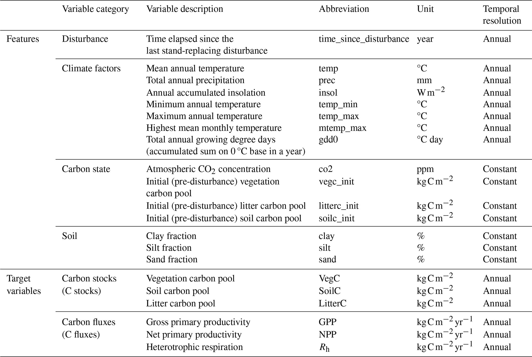
The emulation process was formulated as a supervised learning regression problem, where the features X_i (predictor variables) and targets y_j (outputs) were derived from data generated by the process-based model. The modeling task was to predict either (a) carbon stocks (C stocks) in kg C m⁻², including vegetation carbon (VegC), soil carbon (SoilC), and litter carbon (LitterC), or (b) carbon fluxes (C fluxes) in $\mathrm{kg}\mathrm{C}{\mathrm{m}}^{-\mathrm{2}}{\mathrm{yr}}^{-\mathrm{1}}$, including gross primary productivity (GPP), net primary productivity (NPP), and heterotrophic respiration (R_h), for any given grid cell. We trained separate multi-output regressors for each prediction task (C stocks or C fluxes), as the performance of a single multi-task model was found to be inferior and is not presented here.

We used 15 features as inputs to train the emulators. These included variables related to climate, carbon states prior to a stand-replacing event, soil attributes, and a disturbance timer that tracks the time elapsed since the last stand-replacing disturbance (Table 1). As our emulation application was designed to model forest regrowth following a clear-cut event within LandSyMM, we have included a feature called “time since the last disturbance” (in years) to track forest recovery. Within LandSyMM, this feature will be reset to zero whenever a clear-cut is performed. The input features were aggregated to an annual time step. While some LPJ-GUESS processes operate at finer temporal resolutions (e.g., daily updates for phenology and soil dynamics), key carbon fluxes, such as allocation, are computed annually. Our goal was to develop an emulator that accurately captured interannual variability in carbon dynamics under future climate scenarios while avoiding the complexity and noise associated with higher-frequency inputs. To retain essential intra-annual climate signals relevant to carbon responses, such as the effects of seasonality on productivity, we included variables such as the total annual growing degree days above 0 °C (gdd0). This approach balances model simplicity with the need to represent critical climate-driven processes affecting carbon dynamics.

Table 1 Features and target variables.

2.2.1 Random forest

We developed random forest (RF) regressors (Breiman, 2001) using the scikit-learn Python library's implementation of the RandomForestRegressor (Pedregosa et al., 2011). Mean squared error (MSE) was used as the criterion for evaluating the quality of a decision split. The RF model employed a bootstrap strategy, where training samples were drawn with replacement to fit each tree. A fixed random seed (seed = 42) was used to ensure reproducibility. RF-selected hyperparameters were optimized via grid search, with the selected values and final best settings presented in Table S1 in the Supplement.

2.2.2 Neural network

We developed neural network (NN) regressors using the TensorFlow and Keras libraries (Chollet, 2015; TensorFlow developers, 2024), constructing a fully connected feed-forward neural network. The architecture included an input layer corresponding to the feature space, followed by a series of hidden layers characterized by the number of neurons, activation function, and dropout rate. NN-selected hyperparameters were optimized via grid search, with the selected values and final best settings presented in Table S2.

The output layer consisted of three distinct nodes, each corresponding to one of the target variables (either VegC, SoilC, and LitterC for the C stock regressor or GPP, NPP, and R_h for the C flux regressor). Each output node employed a linear activation function, producing a scalar value for the respective C stock or C flux. The model was compiled using the Adam optimizer (Kingma and Ba, 2017) and the MSE as the loss function. The model was trained for up to 1000 epochs, with an early stopping callback monitoring the validation loss with a patience of 10 epochs. The training process was stopped early when no improvement in validation loss was observed, and the best weights were restored. We used a seed number (seed = 42) to initialize the weights and bias and ensure reproducibility of our results.

The input features were normalized using the MinMax scaler from the scikit-learn library (Eq. 1) to ensure all variables were on a comparable scale, thereby accelerating convergence during training.

$$\begin{array}{}\text{(1)}& X_{\text{scaled}}={\displaystyle \frac{X-X_{\text{min}}}{X_{\text{max}}-X_{\text{min}}}},\end{array}$$

where X_scaled is the normalized value, X is the original value, X_min is the minimum value of the feature, and X_max is the maximum value of the feature.

For NN predictions, we applied a post-processing step to enforce non-negativity in predicted C stocks by replacing all negative values with zero, as negative predictions are not meaningful in this context. This step was not necessary for RFs, which naturally avoid producing negative values due to their structure. Predictions for C fluxes were not post-processed, as they can accept negative values representing flux to the ecosystem in LPJ-GUESS. This approach ensures that all predictions remain physically interpretable.

2.3 Evaluation

The performance of the emulator was evaluated using three metrics: normalized root mean square error (NRMSE), relative bias, and the coefficient of determination (R²). These metrics were computed for each target variable to assess the emulators' predictive accuracy. The NRMSE (Eq. 2) is a normalized version of the root mean square error, scaled by the range of the observed values. The relative bias (Eq. 3) quantifies the systematic error between the predicted and true values as a percentage, and the R² (Eq. 4) indicates the proportion of variance in the true values explained by the emulators.

$$\begin{array}{}\text{(2)}& {\displaystyle }\text{NRMSE}={\displaystyle \frac{\sqrt{\frac{\mathrm{1}}{n}{\sum }_{i=\mathrm{1}}^n(y_i-{\widehat{y}}_i{)}^{\mathrm{2}}}}{max\left(y_i\right)-min\left(y_i\right)}}\text{(3)}& {\displaystyle }\text{Relative bias}={\displaystyle \frac{{\sum }_{i=\mathrm{1}}^n{\widehat{y}}_i-y_i}{{\sum }_{i=\mathrm{1}}^n{y}_i}}\cdot \mathrm{100}\text{(4)}& {\displaystyle }{R}^{\mathrm{2}}=\mathrm{1}-{\displaystyle \frac{{\sum }_{i=\mathrm{1}}^n(y\mathrm{|}i-{\widehat{y}}_i{)}^{\mathrm{2}}}{{\sum }_{i=\mathrm{1}}^n(y\mathrm{|}i-{\stackrel{\mathrm{‾}}{y}}_i{)}^{\mathrm{2}}}}\end{array}$$

In these equations, y_i represents the “true” values as simulated by LPJ-GUESS, ${\stackrel{\mathrm{‾}}{y}}_i$ is the average of all the “true” values y_i, ${\widehat{y}}_i$ denotes the predicted values from the emulator, and n is the number of observations.

The NRMSE provides a normalized error magnitude, enabling comparison across different target variables. Relative bias offers insight into systematic deviations between predictions and true values, while R² indicates the goodness of fit. To evaluate the spatial generalization of the emulator, these metrics were calculated on a test set of grid cells not used during training or validation (see Sect. 3.2). In addition, the emulator's ability to extrapolate was tested by applying it to climate scenarios not included in the training or validation phases.

2.4 Explainable machine learning

Understanding ML model predictions is essential for evaluating their reliability and gaining insights into the factors driving the predictions. In this study, we complemented the evaluation of our models by incorporating SHAP (Shapley additive explanations) values analysis. SHAP is a method based on cooperative game theory used to increase transparency and interpretability of ML models, available in the SHAP Python library (Lundberg and Lee, 2017). SHAP values indicate the most influential features and the direction in which changes in feature values may affect the predicted output. This technique was chosen due to its model-agnostic nature, allowing for consistent interpretability across different algorithms. SHAP assumes feature independence, an assumption often violated in environmental data due to strong correlations among climate variables (Aas et al., 2021). To address this, we adopted a grouping approach (Au et al., 2022), analyzing correlated features through aggregated SHAP values. Specifically, we organized features into four distinct groups based on their correlation patterns, (1) initial carbon pools (soilc_init, litterc_init, vegc_init), (2) climate (temp, insol, temp_min, temp_max, mtemp_max, gdd0), (3) soil properties (clay, silt, sand), and (4) precipitation, which showed no significant correlation with other features. While this approach improves robustness and interpretability under multicollinearity, it reduces feature-level specificity and limits the ability to assess individual feature value effects on model predictions.

To reduce computational time, the SHAP analysis was conducted on a randomly sampled subset of the test dataset (n=500), drawn across grid cells and time steps from the predictions made using the MPI-ESM1-2-HR forcing data for the historical period and climate scenarios (RCP2.6, RCP4.5, RCP7.0 and RCP8.5).

2.5 Computational gain

To evaluate the computational efficiency of our emulators, we compared the execution time of the RF and NN models against the original LPJ-GUESS model. The timing for the emulators encompassed model and data loading, as well as prediction phases for both carbon stocks and fluxes. We quantified the computational efficiency gain using Eq. (5).

$$\begin{array}{}\text{(5)}& \text{gain}={\displaystyle \frac{t_{\text{LPJ-GUESS}}-(t_{\text{cstocks}}+t_{\text{cfluxes}})}{t_{\text{LPJ-GUESS}}}}\cdot \mathrm{100},\end{array}$$

where gain is the computational gain, t_LPJ-GUESS is the baseline execution time (LPJ-GUESS model), t_cstocks is the execution time of the emulator for carbon stock predictions, and t_cfluxes is the execution time of the emulator for carbon flux predictions. We calculated this efficiency metric separately for both the RF and NN models. It is important to note that while LPJ-GUESS simulates all output variables simultaneously, our emulation approach requires separate models for C fluxes and C stocks. Therefore, we summed the execution times of both task-specific emulators to ensure a fair comparison with the LPJ-GUESS runtime.

LPJ-GUESS's computational demand scales quasi-linearly with the number of simulated model grid cells and years, as each pixel is processed independently. For our benchmark, we estimated the computational gain using predictions for a 165-year historical period (1850–2015) simulated with the climate of the MPI-ESM1-2-HR climate model. While this period was selected for practical reasons in our calculations, it is also a widely used simulation period in climate modeling studies. We used 344 grid cells from the validation set for this comparison, expecting that this representative set would capture runtime variations due to differences in the number of simulated woody PFTs and soil-permeable depth across grid cells. For the LPJ-GUESS simulation, we excluded the spin-up period from the timing, instead initializing the historical simulations from a pre-computed state file.

We excluded the time required for generating the training data, training and evaluating the emulators, and the initial development of the LPJ-GUESS model, as these steps occur only during the development phase and are not part of the emulators' operational use. Our focus was on comparing the runtime efficiency of the trained emulators against LPJ-GUESS for making predictions, which reflects their typical practical application. It should be noted that the actual time saved depends on the machine infrastructure and software and may therefore differ from the theoretical estimate.

3 Data

3.1 Data generation

We conducted multiple scenario simulations using the LPJ-GUESS model, focusing specifically on forest grid cells. These cells were identified through an initial global simulation of potential natural vegetation, followed by classification into distinct vegetation types (biomes) based on PFT abundances and leaf area index, as described by Smith et al. (2014). From the globally simulated forest grid cells, we employed a stratified sampling method to ensure balanced representation across eight distinct forest biomes: tropical rainforest, tropical deciduous forest, tropical seasonal forest, boreal evergreen forest, boreal deciduous forest, temperate broadleaved evergreen forest, temperate deciduous forest, and temperate and boreal mixed forests. A total of 15 % of the forest grid cells were selected for emulator development, resulting in a dataset of 3448 grid cells.

The sampled grid cells were then randomly divided into training (80 %), validation (10 %), and test (10 %) sets, with an equal number of cells selected from each biome for each set (Fig. 1). This approach minimizes the risk of over-representing any particular forest biome during training and evaluation, thereby reducing bias in the ML models (Sun et al., 2023), as biophysical properties and climate change responses can vary significantly between them. The training set was used to update the ML model parameters, while the validation set guided hyperparameter tuning and monitoring for overfitting. The test set was reserved for evaluating emulation performance on grid cells unseen during training and validation. By using distinct grid cells for training, validation, and testing, we aimed to assess the robustness of the spatial generalization of the emulation.

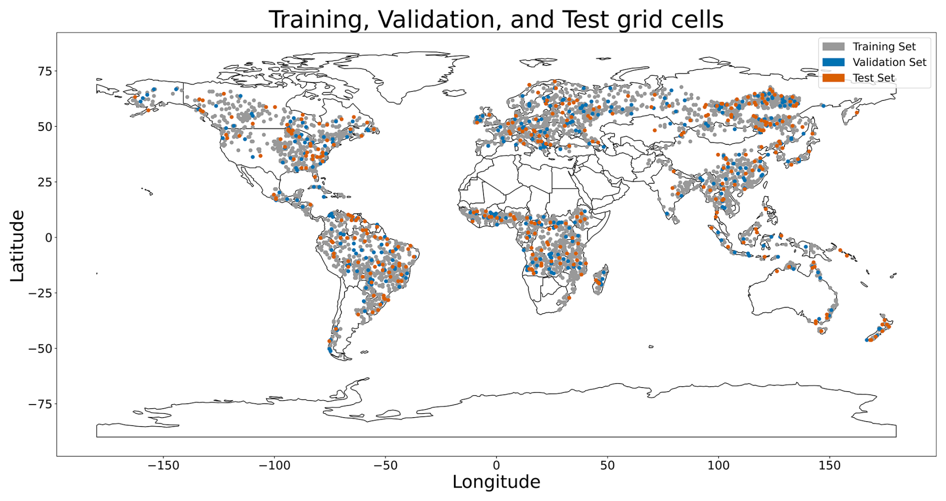
Figure 1 Spatial distribution of the sampled grid cells for training, validation, and testing.

The LPJ-GUESS simulations were driven by climate scenarios derived from the Coupled Model Intercomparison Project Phase 6 (CMIP6; Eyring et al., 2016), bias-corrected for the Inter-Sectoral Impact Model Intercomparison Project phase 3 (ISIMIP3) (Lange, 2019; Lange and Büchner, 2021). We used temperature, precipitation, and solar radiation data from five Earth system models (ESMs): IPSL-CM6A-LR, MPI-ESM1-2-HR, MRI-ESM2-0, GFDL-ESM4, and UKESM1-0-LL, covering four Representative Concentration Pathways (RCPs) – RCP2.6, RCP4.5, RCP7.0, and RCP8.5. Nitrogen deposition data used in the simulations were sourced from Lamarque et al. (2013). Details of the LPJ-GUESS simulation protocol, including model version, modifications, experimental setup, and forcing data, are available in the “Code and data availability” section and Sect. S1 in the Supplement.

3.2 Data pre-processing

To make the emulator model-agnostic, we pre-processed the raw LPJ-GUESS simulation outputs by taking the ensemble mean of the five ESMs for training. The test set was used to assess the emulation performance on data not used during training and validation. For testing, we used the LPJ-GUESS simulation outputs from each climate model individually, rather than the ensemble mean, and included climate change scenarios not used during training and validation. The datasets are described in Table 2.

Table 2 Description of the training, validation, and test datasets. The datasets covered the historical (1850–2014) and future period (2015–2100).

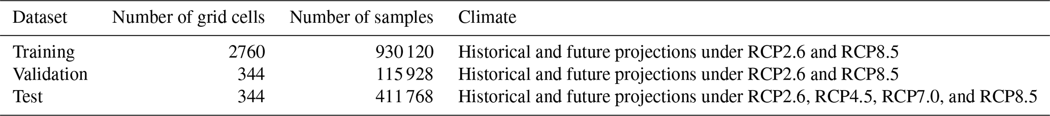
The number of samples refers to the total number of data points in each dataset, calculated by multiplying the number of grid cells by the number of time points (years) in the climate data for each set. Historical data contain 165 years, and the future period contains 86 years. The training and validation sets use ensemble data from five climate models. The test set uses individual simulations from three separate climate models (GFDL-ESM4, MPI-ESM1-2-HR, and MRI-ESM2-0) rather than an ensemble, so we multiplied the future period length by 3.

4 Results

4.1 Emulator performance

The emulators demonstrated a significant reduction in simulation execution time. For the validation set, LPJ-GUESS required 5765 s to run, while the RF and NN emulators completed the simulation in just 1.3 and 2.8 s, respectively, on a single-processor machine. However, as LPJ-GUESS simulations are typically run in parallel on high-performance computing systems, we also calculated runtime per grid cell by dividing the total runtime by the 344 grid cells used in this analysis. This yielded an average runtime reduction of 95 % with the emulators compared to the original model.

We evaluated the emulators' ability to replicate carbon dynamics as simulated by LPJ-GUESS using the test dataset. The emulators were trained on historical climate data and projections from the RCP2.6 and RCP8.5 scenarios. Performance was assessed over the historical period and across four RCP scenarios – RCP2.6, RCP4.5, RCP7.0, and RCP8.5 – capturing a broad range of potential future climate conditions.

4.1.1 Carbon stocks

Overall, both the NN and RF models demonstrated good performance across the different carbon pools and RCP scenarios. As shown in Table 3, the emulators were able to generalize to LPJ-GUESS outputs produced with climate projections (RCP4.5 and RCP7.0) that were not included in the training data, without a significant decline in performance compared to the training scenarios (RCP2.6 and RCP8.5). This indicates that the emulators can generalize across intermediate emission scenarios, which fall within the range defined by the low (RCP2.6) and high (RCP8.5) extremes used during training. However, extrapolation beyond this range would require additional training and evaluation, as black-box models are not inherently robust in extrapolation tasks (Muckley et al., 2023). The NRMSE values were consistently low, ranging from 0.01 to 0.12 across target variables and scenarios, indicating a high degree of predictive accuracy. The RF underestimated C stocks for most of the RCP scenarios. Overall, the NN model exhibited consistently smaller relative bias compared to the RF model, especially in the prediction of VegC, except for SoilC. Among the carbon stock variables, SoilC was predicted with the greatest accuracy by both NNs and RFs, exhibiting the lowest error and highest R² values. Overall, the NN emulator outperformed the RF emulator across the RCP scenarios and target variables.

Table 3 Performance metrics of random forest (RF) and neural network (NN) emulators for predicting carbon stocks in forest ecosystems, including vegetation carbon (VegC), soil carbon (SoilC), and litter carbon (LitterC), across four different climate projections.

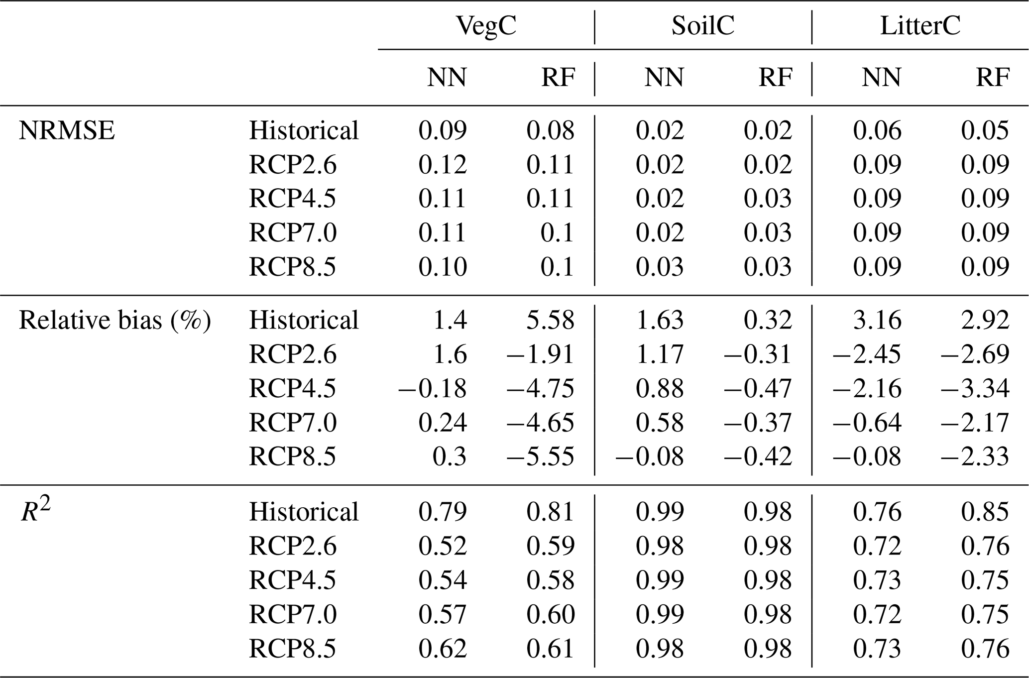
Figure 2 illustrates how well the emulators captured the temporal dynamics of carbon pools across different biomes after a stand-replacing disturbance. Overall, both emulators closely approximated the process-based simulations from the historical period into future projections across RCPs. However, in boreal forests, the RF regressor tends to overestimate VegC during the early years of forest regrowth following a disturbance, while underestimating it by the end of the 21st century across all RCPs. Similarly, the NN regressor showed this pattern in tropical forests, where it also struggled to capture the undulations in VegC likely associated with tree age-related mortality. In temperate and mixed forests, both emulators accurately represented initial regrowth but failed to capture VegC accurately by the end of the 21st century.

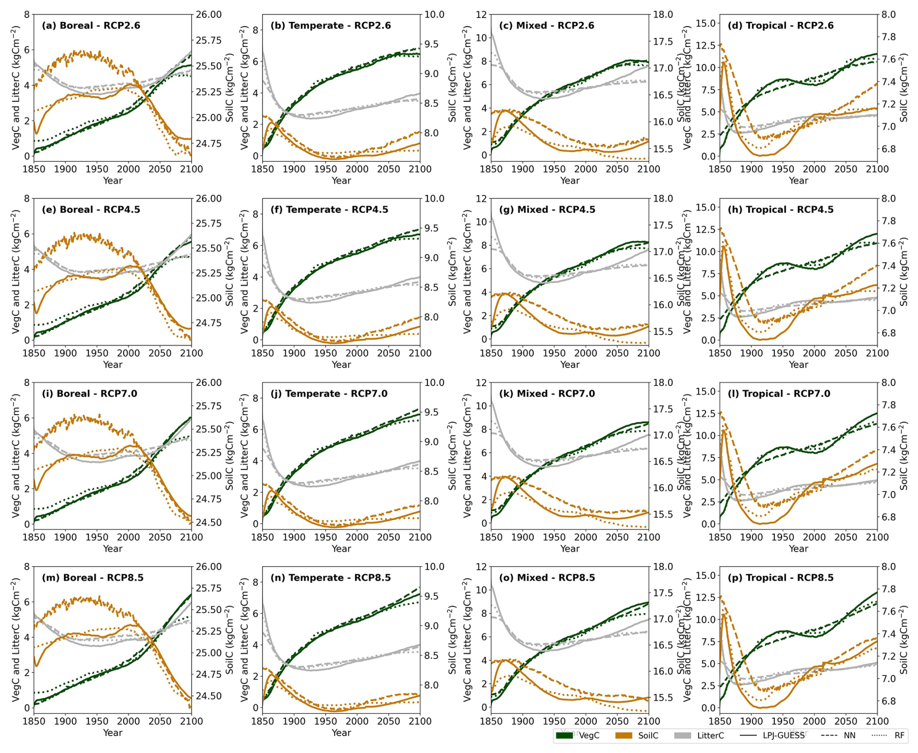
Figure 2 Biome-specific average carbon stock trajectories across a range of climate change projections following a stand-replacing disturbance in 1849. Solid lines represent LPJ-GUESS simulations, while dashed and dotted lines indicate emulator predictions. The predictions are averaged across three Earth system models (GFDL-ESM4, MPI-ESM1-2-HR, MRI-ESM2-0) for the test set.

Both emulators underestimated the peak in LitterC following a disturbance and toward the end of the time series, particularly in temperate and mixed forests. SoilC remains relatively stable over time, with the RF emulator capturing these subtle changes more effectively than the NN emulator, particularly in boreal and tropical forests.

Figure 3 presents the spatial patterns of emulator errors in carbon stock predictions. The RF and NN emulators exhibited distinct spatial errors for VegC. The RF generally underestimated VegC, except for significant overestimation in central Asia. In contrast, the NN tends to overestimate VegC in boreal evergreen forests in central Asia and in temperate broadleaved evergreen forests, particularly in eastern Asia, the southeastern United States, and southern Europe. Additionally, the NN overestimated VegC at the borders of forest biomes, including boreal forests in Russia and North America. Both emulators demonstrated high accuracy in SoilC predictions, with minimal spatial error variation across regions. For LitterC, the RF and NN models showed similar error patterns in tropical forests, although the NN model tends to produce higher errors, especially in eastern China.

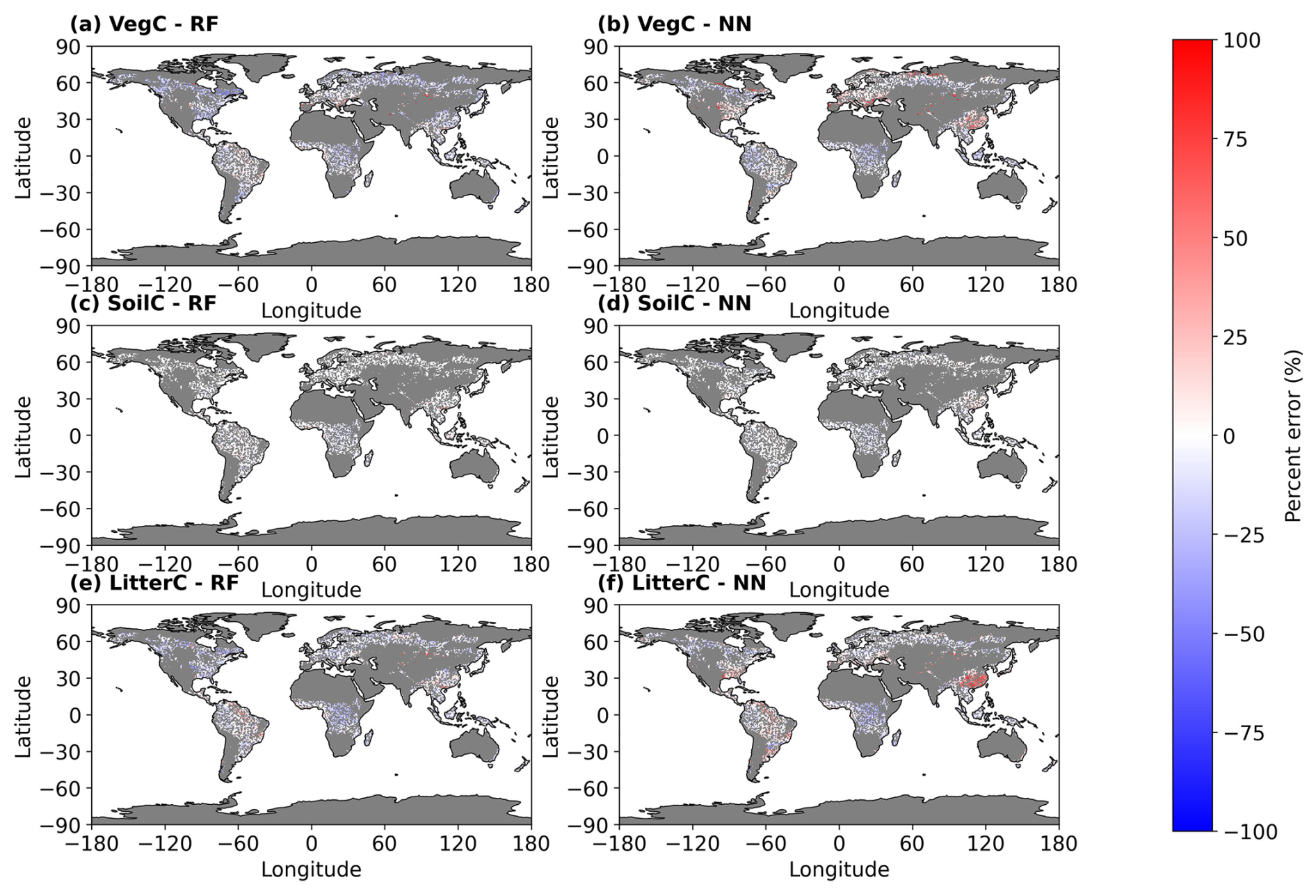
Figure 3 Average percent error in vegetation carbon (VegC), soil carbon (SoilC), and litter carbon (LitterC) stocks (kg C m⁻²) predicted by random forest (RF) and neural network (NN) emulators, compared to LPJ-GUESS model outputs. Errors are averaged over the period 2070–2100. The predictions are based on simulations using climate data from the MPI-ESM1-2-HR Earth system model under the RCP8.5 scenario. The map illustrates predicted errors across all LPJ-GUESS forested grid cells, including those used for training, validation, and testing. Gray pixels indicate non-forested areas.

4.1.2 Carbon fluxes

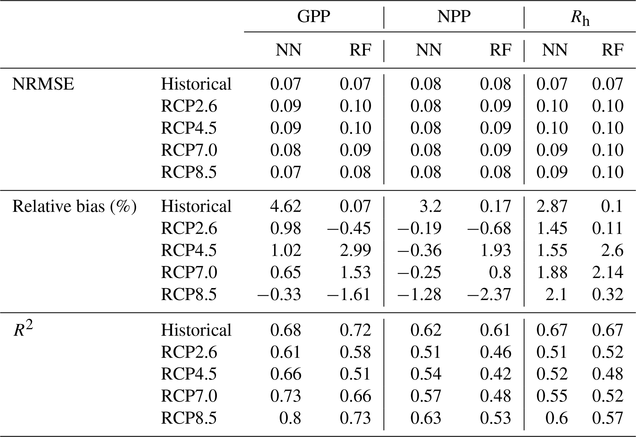
Similar to the C stocks, the NN and RF emulators showed good agreement with the LPJ-GUESS simulations in predicting GPP, NPP, and R_h under the historical period and four RCPs. Both emulators successfully generalized to RCPs not used during the training process. The NRMSE values were consistently low, ranging from 0.07 to 0.10 for both emulators across all carbon flux variables and RCP scenarios, indicating accurate predictions (Table 4).

Overall, the RF model outperformed the NN during the historical period, exhibiting lower error and more accurate predictions. However, performance differences between the models became less pronounced for the RCP scenarios. In the warmer RCP scenarios, the NN showed a slight improvement over the RF model, with the exception of R_h, where the RF model maintained a marginal advantage. This suggests that while the RF model excels under historical conditions, the NN may adapt better to projected warmer climates, providing competitive performance across most C fluxes.

Table 4 Performance metrics of random forest (RF) and neural network (NN) emulators for predicting carbon fluxes in forest ecosystems, including gross primary productivity (GPP), net primary productivity (NPP), and heterotrophic respiration (R_h), across four different climate projections.

The emulators reasonably captured the temporal dynamics of C fluxes across different biomes following a stand-replacing disturbance, as shown in Fig. 4. However, some discrepancies were observed with the RF emulator's predictions of GPP and NPP toward the end of the century across various RCPs and forest types. The NN emulator systematically overestimated GPP in boreal forests. Figure 5 shows the spatial variation in the emulators' errors for C fluxes. The average error for the period 2070–2100 was small, and the error patterns were quite similar between the emulators.

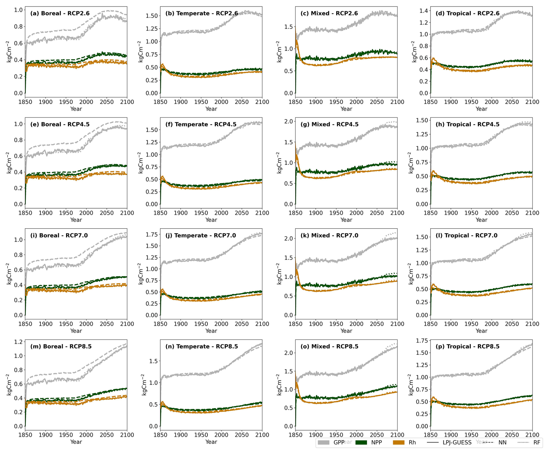
Figure 4 Biome-specific average carbon fluxes across four climate projections (columns) following a stand-replacing disturbance at the year 1849. Solid lines indicate LPJ-GUESS simulations, and dashed lines indicate emulators. The predictions are averaged across three Earth system models (GFDL-ESM4, MPI-ESM1-2-HR, MRI-ESM2-0) for the test set.

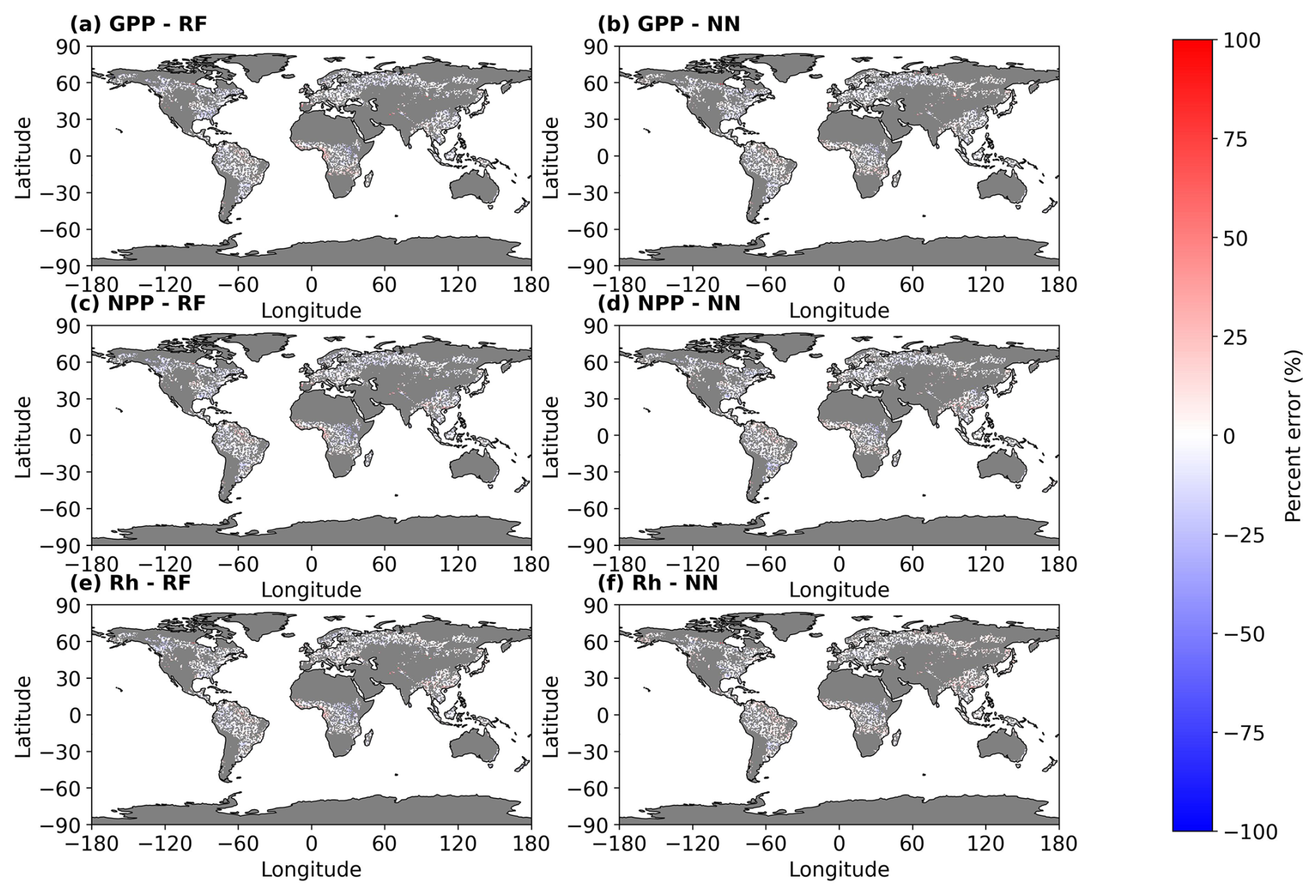
Figure 5 Average percent error in gross primary productivity (GPP), net primary productivity (NPP), and heterotrophic respiration (R_h) ($\mathrm{kg}\mathrm{C}{\mathrm{m}}^{-\mathrm{2}}{\mathrm{yr}}^{-\mathrm{1}}$) predicted by random forest (RF) and neural network (NN) emulators, compared to LPJ-GUESS model outputs. Errors are averaged over the period 2070–2100. The predictions are based on simulations using climate data from the MPI-ESM1-2-HR Earth system model under the RCP8.5 scenario. The map illustrates predicted errors across all LPJ-GUESS forested grid cells, including those used for training, validation, and testing. Gray pixels indicate non-forested areas.

4.2 Emulator explainability

We extended our emulation assessment by presenting an analysis of model explainability through SHAP values. This technique provided complementary insights into the inner workings of our ML-based emulators, indicating which groups of features were most influential in driving predictions.

For carbon stock predictions, the grouped SHAP analysis indicated similar feature importance rankings for both the RF and NN emulators, with only minor differences in the magnitude of feature group contributions to model outputs (Fig. 6). Precipitation and soil attributes emerged as the least influential factors, though these features exhibited slightly higher sensitivity in the NN emulators. Variables associated with the initial carbon state prior to disturbance emerged as the most influential across all carbon stock variables and emulators. Temporal features, such as atmospheric CO₂ concentration and time since disturbance, generally ranked second in importance, except for soil carbon predictions, where climate variables were the second most significant factor.

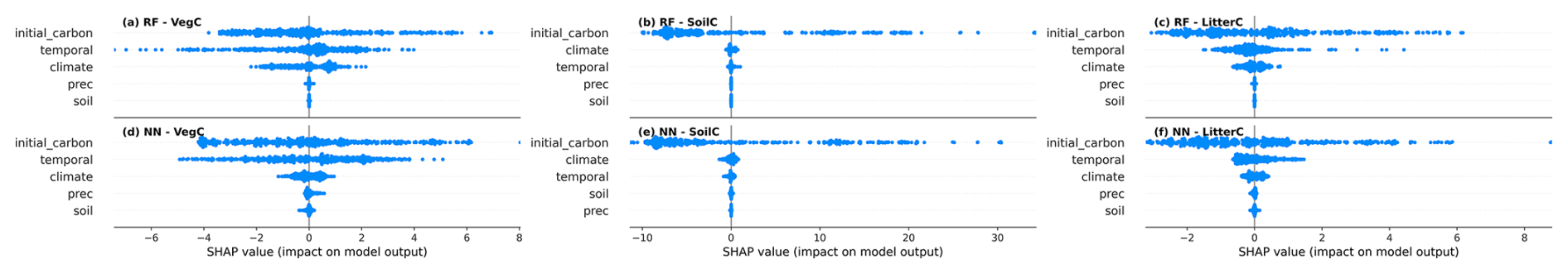
Figure 6 SHAP values for grouped features in carbon stock predictions, including vegetation carbon (VegC), soil carbon (SoilC), and litter carbon (LitterC), using (a–c) random forest (RF) and (d–f) neural network (NN) emulators. The y axis lists feature groups ranked by importance, where correlated features were grouped as follows: initial carbon (soilc_init, litterc_init, vegc_init), climate (temp, insol, temp_min, temp_max, mtemp_max, gdd0), and soil (clay, silt, sand). Precipitation (prec) was not correlated with other features. The x axis displays SHAP values, which represent the impact of each feature group on model predictions. Positive SHAP values indicate an increase in predicted carbon stock, while negative values indicate a decrease. Each point represents a dataset instance, with its position along the x axis reflecting the feature's contribution to that prediction.

Notably, for SoilC, variables beyond the initial carbon state contributed minimally to model outputs, in contrast to patterns observed for other carbon stock components.

For carbon flux predictions, the RF and NN emulators exhibited distinct feature importance patterns (Fig. 7). SHAP values from the RF emulator identified the initial ecosystem carbon state as the most influential feature group. In contrast, the NN emulator emphasized the joint contribution of atmospheric CO₂ concentration and time since disturbance for gross primary production (GPP), while climate variables were most influential for both net primary production (NPP) and heterotrophic respiration (R_h).

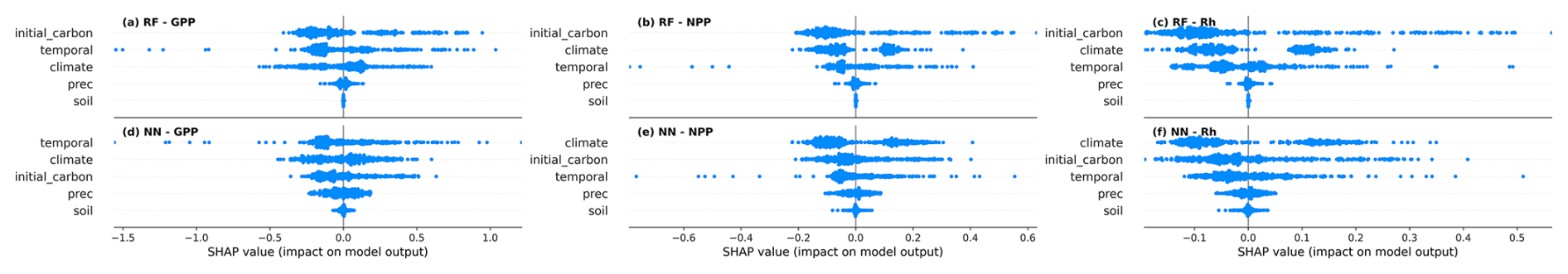
Figure 7 SHAP values for grouped features in carbon flux predictions, including vegetation carbon (GPP), soil carbon (NPP), and litter carbon (R_h), using (a–c) random forest (RF) and (d–f) neural network (NN) emulators. The y axis lists feature groups ranked by importance, where correlated features were grouped as follows: initial carbon (soilc_init, litterc_init, vegc_init), climate (temp, insol, temp_min, temp_max, mtemp_max, gdd0), and soil (clay, silt, sand). Precipitation (prec) was not correlated with other features. The x axis displays SHAP values, which represent the impact of each feature group on model predictions. Positive SHAP values indicate an increase in predicted carbon stock, while negative values indicate a decrease. Each point represents a dataset instance, with its position along the x axis reflecting the feature's contribution to that prediction.

5 Discussion

We developed an ML emulation approach to approximate LPJ-GUESS simulations of carbon dynamics in forest ecosystems. Both RF and NN emulators accurately reproduced the process-based output. However, differences in their generalization to climate scenarios and ML explainability revealed distinct strengths and weaknesses inherent to each model type.

5.1 Emulator performance

Overall, the RF emulator exhibited lower bias during the historical period and outperformed the NN in predicting R_h and in capturing small changes in SoilC. The NN model, on the other hand, outperformed the RF emulator in predicting VegC and under the warmer RCP scenarios. It also showed superior performance for R_h predictions in mixed forests toward the end of the century. These findings align with prior studies comparing these two ML models, which have found negligible differences in their performance (Ahmad et al., 2017), although some reported marginal improvements by RF in regression tasks, especially in tabular data (Nawar and Mouazen, 2017; Grinsztajn et al., 2022). Ultimately, the performance of ML algorithms varies significantly depending on the dataset's dimensionality and the specific application. NNs generally require larger datasets to achieve optimal performance, while RFs are more data-efficient, needing fewer samples for training and minimal hyperparameter tuning. Therefore, the choice of algorithm should always be evaluated in the context of the specific application at hand.

It should also be noted that training emulators on climate projections from ESMs was not our initial approach. We first experimented with stylized climate change scenarios for training, following the methodology of Franke et al. (2020), which used factorial combinations of temperature, precipitation, and CO₂ levels to emulate crop productivity. Our hypothesis was that training the emulators on a factorial experiment, with independent variations in temperature, precipitation, and atmospheric CO₂ concentration, would allow them to learn physical relationships between inputs and outputs and subsequently generalize well to realistic climate projections. However, the trained models failed to extrapolate effectively to the real CMIP6 climate scenarios. An explanation for this is that the stylized scenarios produced combinations of temperature, precipitation, and atmospheric CO₂ concentrations too far removed from those expected in realistic settings. This could have biased the models, reducing their effectiveness when faced with actual climate projections. To mitigate this, we also explored a two-step training approach using the NN emulator: pre-training on the factorial dataset followed by fine tuning on RCP scenarios. However, this approach led to two outcomes. Either (i) the model became biased toward the factorial data and performed poorly on realistic RCP scenarios, or (ii) flexible weight adaptation during fine tuning effectively erased the pre-trained knowledge. Both issues significantly undermined the benefits of pre-training and increased training time. This highlights a fundamental limitation of purely ML-based emulators: they lack the structural constraints of process-based models and may fail to generalize across divergent data distributions. Future work could address this through pre-processing strategies to better balance the training datasets by, for example, oversampling RCP-like examples to counteract the imbalance or including physical constraints in a hybrid approach. However, implementing such flexible emulation strategies was beyond the scope of this study.

Despite these challenges, our ML emulators remain highly effective for their intended purpose. By training on physically plausible RCP trajectories at each grid cell, the models were able to learn realistic covariances among climate drivers.

5.2 Emulator explainability

The selection of predictive models in scientific modeling often overlooks explainability, especially when high predictive accuracy is a primary objective. However, explaining ML models is important for diagnosing model biases, managing multi-objective trade-offs, and mitigating unexpected outcomes in practical applications (Muckley et al., 2023).

Although direct comparisons between ML explainability methods and sensitivity analyses of process-based models such as LPJ-GUESS are inherently challenging due to structural and conceptual differences, we use SHAP values to examine the behavior of the emulation. Specifically, we interpret SHAP values for input features corresponding to LPJ-GUESS forcing, namely, climate variables and atmospheric CO₂ concentrations, drawing on insights from prior LPJ-GUESS sensitivity studies (Ahlström et al., 2013, 2017; Piao et al., 2013). We explicitly exclude comparisons with LPJ-GUESS parameter sensitivity analyses, as these are not directly applicable within the emulation framework adopted here.

In this study, the most important features varied across models and prediction tasks, reflecting how different ML approaches prioritize distinct aspects of the input data. Our results demonstrate that the initial ecosystem carbon state was the most important feature for predicting carbon stock variables in both the RF and NN emulators. Initial carbon pool sizes not only play a critical role in determining potential carbon loss under future warming scenarios (Todd-Brown et al., 2014), but may also serve as implicit indicators of forest biome characteristics in the context of emulation. Because spatial proxies such as geographic coordinates were excluded from the model inputs, baseline carbon pools may have indirectly captured biome-specific carbon allocation strategies. For example, tropical forests tend to store more carbon above ground, whereas boreal forests allocate a larger fraction below ground.

Beyond initial carbon conditions, both models identified time since disturbance and atmospheric CO₂ concentration, grouped as temporal features, as key drivers of forest regrowth and carbon dynamics. Time since the last stand-replacing disturbance likely served as a proxy for forest age, which plays a pivotal role in carbon accumulation. Younger forests typically act as stronger carbon sinks due to rapid growth, while older forests tend to exhibit slower carbon uptake as they reach maturity (Cook-Patton et al., 2020; Pugh et al., 2019). Additionally, elevated levels of LitterC may be predicted in the years immediately following disturbance – i.e., when time since disturbance is low – reflecting biomass transfer from vegetation to litter pools (Zhang et al., 2024). Furthermore, it is important to consider the differences between emulators built for crops and for forest ecosystems. In crops, factors such as time since disturbance typically play a less direct role, as the annual cycle of harvesting and replanting limits the long-term effects of disturbances. Crops are more strongly influenced by climate and CO₂ levels. In contrast, trees are significantly affected by legacy effects and timing of events, and this disparity highlights the need for emulators to incorporate these variables when applied to forest ecosystems.

Ahlström et al. (2017) demonstrated that climate biases influence LPJ-GUESS-simulated vegetation and soil carbon pools with comparable magnitude over time, although long-term soil carbon uptake tends to exhibit lower sensitivity. In line with this, our SHAP analysis indicates that VegC predictions are more responsive to climate variables than SoilC. The limited influence of climate on SoilC predictions may reflect the inherently slow turnover of this carbon pool. Within our simulation time frame, the most influential predictor was the initial carbon stock after the spin-up period, with climate-driven changes contributing only marginally in absolute terms. The inclusion of the highly correlated initial SoilC pool likely simplified the learning task, potentially inflating emulator accuracy metrics for SoilC. This strong dependence on initial conditions may also signal reduced sensitivity to environmental drivers, thereby constraining the emulator's capacity to represent long-term soil carbon responses to climate change. Future work could address this limitation by incorporating regularization strategies aimed at mitigating over-reliance on initial carbon states.

Although precipitation ranked low in importance across most emulators and target variables, it did exhibit an influence on carbon flux predictions. This finding is consistent with a prior study reporting a positive global relationship between GPP and precipitation in vegetation models such as LPJ-GUESS, particularly in tropical ecosystems (Piao et al., 2013). The observed sensitivity of carbon flux predictions to atmospheric CO₂ concentration and time since disturbance also reflects established experimental and modeling literature suggesting that elevated CO₂ can enhance NPP and forest carbon uptake (Ahlström et al., 2012; Piao et al., 2013).

Other climate-related variables – such as temperature, gdd0, and insolation – also emerged as important drivers, particularly for VegC and carbon flux variables. In the NN emulator, climate features ranked highest in importance for NPP and R_h and second – after temporal features – for GPP. As noted in LPJ-GUESS sensitivity studies, a longer and warmer growing season tends to enhance productivity in boreal and temperate regions with ample moisture (Ahlström et al., 2012). In temperate forests, however, the net impact of warming is more nuanced, balancing the benefits of an extended growing season against the drawbacks of increased summer soil moisture stress (Piao et al., 2013). In our emulation framework, such seasonal dynamics could have been captured by the annually accumulated growing degree days. Closer inspection of the individual feature contributions (Fig. S2 in the Supplement) confirms that gdd0 and temperature are among the most influential predictors of carbon fluxes in the NN emulator. It is important to note that, due to the use of an annual time step for input features, some LPJ-GUESS sensitivities to intra-annual climate cannot be fully captured in our simulations. However, we argue that the selected input features are well-suited for capturing the interannual variability in carbon dynamics for our intended application, as demonstrated in the emulator evaluation.

NNs also showed a slightly greater sensitivity to soil properties, although still modest, in all predictions of carbon stocks and fluxes (except SoilC). This is consistent with expectations from LPJ-GUESS, which provides only a coarse representation of soil properties.

Overall, our analysis suggests that the emulators capture key sensitivities present in LPJ-GUESS, albeit in different ways. However, interpreting the behavior of ML models remains challenging when input features are highly correlated, as only coarse groups, rather than individual features, can be analyzed. In addition, structural differences between LPJ-GUESS and the ML emulators make direct comparisons of feature importance difficult. Future emulator designs could benefit from the integration of physical constraints or process knowledge to better reflect plausible relationships between forcing and carbon dynamics, thereby improving the robustness and reliability of the emulation.

5.3 Comparison to previous studies

A common approach in emulating spatially resolved ecosystem variables, particularly with statistical methods, involves developing multiple emulators tailored to specific plant functional types (PFTs), crop types, fire regimes, or biomes (Ahlström et al., 2013; Ekholm et al., 2024; Franke et al., 2020). This strategy facilitates the approximation of complex ecological functions and has been effective for certain applications. However, we argue that biome-specific emulators may be less suited for modeling future climate scenarios, where biome shifts or changes in forest productivity due to CO₂ fertilization are expected to occur. Fitting the parameters of emulators to specific biomes also risks averaging out regional climate change effects, thereby reducing the model's ability to capture the nuanced interactions that drive ecosystem dynamics at finer scales.

While the development of an LPJ-GUESS emulator is not new, our approach differs from previously developed approaches. Ekholm et al. (2024) emulated the effects of climate change on C stocks as a linear function of global mean temperature changes and atmospheric CO₂ concentrations, with separate applications for each biome, while Ahlström et al. (2013) parameterized a statistical emulator mimicking the LPJ-GUESS results when forced by global temperature and atmospheric CO₂ as sole drivers. Although these approaches are computationally efficient and interpretable, their reliance on linear regression may oversimplify the nonlinear ecological responses to climate change and miss regional climate variations that differently impact biomes. In contrast, our approach proposes a single global emulator that does not rely on spatial proxies, and it is not specific to a certain biome type or PFT. This biome-agnostic design allows the emulator to capture both global and regional climate dynamics without averaging the effects of climate change across biomes. This approach can also more effectively model biome shifts and other complex ecosystem responses to future climate scenarios.

5.4 Emulator application

The emulators developed in this study are lightweight models designed to simulate forest ecosystem carbon dynamics in response to climate change. It is important to note that while the emulators were generally able to reproduce LPJ-GUESS's outputs related to forest carbon dynamics for the employed RCP scenarios, they should not be expected to capture all original model sensitivities, including both parameter sensitivities (e.g., parameters governing vegetation dynamics), and the original model's physical responses (e.g., the response of carbon dynamics to atmospheric CO₂ outside the bounds of training data). Furthermore, ML-based emulators should not be assumed to reliably extrapolate beyond the training data distribution without proper validation. In our study, both models were evaluated on scenarios that, while challenging, were within reasonable bounds of the training conditions. As demonstrated in Lakshminarayanan et al. (2017), NNs extrapolate poorly and uncertainty bounds using ensemble techniques may help to encompass the true function, an approach that could be explored in further development of emulation approaches.

While the emulators can be used directly for rapid simulations of carbon pools and fluxes without the need for solving an optimization problem, they were aimed at integration with LandSyMM. Future work will explore this integration to enable addressing questions related to the forest-based climate change mitigation potential in the context of global environmental change. Specifically, the emulators will provide annual forest productivity and track changes in C stocks and CO₂ emissions following clear-cuts. The land use model within LandSyMM, PLUM, will provide information regarding the timing of clear-cuts and affected grid cells so that the emulator can predict the target variables in the future based on the current state of C stocks, annual climate conditions, and other relevant features. Within LandSyMM's coupled framework, the emulator will act as a computationally efficient substitute for LPJ-GUESS at each coupling interval (e.g., every 5 years), rapidly estimating forest carbon potentials. This removes the need for full 100-year simulations for each scenario iteration. However, to maintain realism in projections, the emulator will not be used to simulate actual carbon outcomes for the next 5 years of predicted land use. Instead, LPJ-GUESS will be employed to simulate carbon dynamics during that period, and the emulator will resume operation in the next coupling cycle.

Future development of the emulator may be required to accommodate additional forestry practices, such as various thinning regimes, specific planted PFTs, or harvest probabilities. The emulator's flexibility means it can be retrained or fine-tuned for different horizontal resolutions, as well as adapted for alternative applications, such as more detailed management strategies.

6 Conclusions

The emulators developed in this study demonstrate the effectiveness of ML methods in accurately capturing the process-based dynamics of forest carbon stocks and fluxes under climate change scenarios. However, the differences in model performance and explainability highlight the trade-offs between the generalization ability and overall accuracy of each model type. The NN's tendency to over- and underestimate target variables is contrasted with its ability to generalize well to warmer climate scenarios by the end of the 21st century and its decision-making that is highly consistent with ecological processes. Nevertheless, we do not discard the use of the RF emulator, particularly due to its overall higher prediction accuracy in the first years following a disturbance event. These findings emphasize the importance of model selection based on the specific task at hand and the trade-offs between accuracy and interpretability in future projections. The potential use of an ensemble model for emulation is also worth considering, as it could combine the strengths of both models while offering the advantage of faster predictions. Moreover, further development of the LPJ-GUESS emulator for LandSyMM could benefit from constraining the emulator with LPJ-GUESS “physics”, which would make it more useful in a broader range of applications.

While the emulation development was nontrivial, the whole approach was developed using standard open-source ML libraries, facilitating replication and subsequent improvement efforts. The integration of such ML approaches into modeling frameworks has the potential to improve forest management optimization, offering a valuable tool for policy planning in the face of climate change.