Quantification of CO₂ hotspot emissions from OCO-3 SAM CO₂ satellite images using deep learning methods

This paper presents the development and application of a deep-learning-based method for inverting CO₂ atmospheric plumes from power plants using satellite imagery of the CO₂ total column mixing ratios (XCO₂). We present an end-to-end convolutional neural network (CNN) approach, processing the satellite XCO₂ images to derive estimates of the power plant emissions, that is resilient to missing data in the images due to clouds or to the partial view of the plume owing to the limited extent of the satellite swath.

The CNN is trained and validated exclusively on CO₂ simulations from eight power plants in Germany in 2015. The evaluation on this synthetic dataset shows an excellent CNN performance with relative errors close to 20 %, which is only significantly affected by substantial cloud cover. The method is then applied to 39 images of the XCO₂ plumes from nine power plants, acquired by the Orbiting Carbon Observatory-3 Snapshot Area Maps (OCO3 SAMs), and the predictions are compared to average annual reported emissions. The results are very promising, showing a relative difference in the predictions to reported emissions only slightly higher than the relative error diagnosed from the experiments with synthetic images. Furthermore, analysis of the area of the images in which the CNN-based inversion extracts the information for the quantification of the emissions, based on integrated-gradient techniques, demonstrates that the CNN effectively identifies the location of the plumes in the OCO-3 SAM images. This study demonstrates the feasibility of applying neural networks that have been trained on synthetic datasets for the inversion of atmospheric plumes in real satellite imagery from XCO₂ and provides the tools for future applications.

1 Introduction

Satellite imagery of the total column average dry-air mole fraction of carbon dioxide (XCO₂) from the Snapshot Area Map (SAM) mode of the Orbiting Carbon Observatory-3 (OCO-3) (Eldering et al., 2019) or the forthcoming CO2M mission (Janssens-Maenhout et al., 2020; Meijer et al., 2023) is pivotal for monitoring carbon dioxide (CO₂) emissions. In the vicinity of large CO₂ anthropogenic sources, such as power plants, satellite images may include CO₂ atmospheric plumes emanating from these sources. From these images, atmospheric inversion approaches can estimate the CO₂ emissions of the sources by analysing the signal intensity of the detected plumes (Nassar et al., 2017; Reuter et al., 2019; Chevallier et al., 2019; Wu et al., 2020; Zheng et al., 2020; Nassar et al., 2022; Chevallier et al., 2022; Cusworth et al., 2021).

Various approaches can be used to determine the emissions underlying the XCO₂ plumes in the satellite imagery. The first technique category relies on traditional atmospheric inversion methods that minimize the misfits between the satellite observations and simulations of the plumes with relatively expensive (Eulerian or Lagrangian) transport models to identify the optimal emission estimate (Pillai et al., 2016; Broquet et al., 2018). The second technique category includes light-weight methods that apply the principle of mass conservation to compute the emissions from the CO₂ enhancement of the emission plume (such as integrated mass enhancements, divergence methods, and cross-sectional flux methods) or compare the observed plume with a Gaussian plume model (Gaussian plume inversions). Light-weight methods rely on wind fields taken, for example, from meteorological reanalysis products. These light-weight methods have been evaluated in several studies (e.g. Varon et al., 2018; Hakkarainen et al., 2024; Danjou et al., 2025; Santaren et al., 2025; Kuhlmann et al., 2024; Danjou et al., 2024). Despite the advancements in CO₂ plume inversion techniques, significant challenges remain, notably, (1) the extraction of plumes from XCO₂ backgrounds, which is hindered by low signal-to-noise ratios due to the large amplitude of background variations associated with the CO₂ natural fluxes and to relatively high noise in the image (due to instrumental errors and to uncertainties in the retrieval of mole fractions from the satellite measurements); (2) the complex process of deducing the source emissions from clearly delineated plumes, which is marred by uncertainties in the corresponding transport and dispersion (i.e. in either the transport modelling or in the wind field and assumptions regarding the vertical structure of the 3D CO₂ plume for the derivation of the effective wind driving the 2D XCO₂ plume in the light-weight analysis; Dumont Le Brazidec et al., 2023); and (3) the reconstruction of emissions from images with a partial view of the plumes due to missing data where there are clouds or gaps in satellite coverage.

Machine learning models have been suggested in response to these obstacles and have been primarily applied to CH₄ and NO₂ images (e.g. Lary et al., 2016; Finch et al., 2022; Jongaramrungruang et al., 2021; Joyce et al., 2023; Kumar et al., 2023). Our previous work (Dumont Le Brazidec et al., 2023, 2024a) pioneered the use of deep learning methodologies, specifically convolutional neural networks (CNNs), for the segmentation and inversion of CO₂ plumes for the estimate of point sources. This approach has demonstrated its efficacy in addressing these challenges when tackling synthetic satellite images with a full coverage of the plumes, i.e. without the loss of observations due to cloud cover or quality control in the limited satellite field of view. This paper is a direct continuation of Dumont Le Brazidec et al. (2024a). Specifically, our approach involves developing a supervised-learning CNN system designed to predict CO₂ emissions using XCO₂ images and ancillary data (such as wind fields, time, and NO₂ images which will be measured by CO2M). This CNN is trained on a synthetic dataset, constructed from model simulations, comprising synthetic XCO₂ fields and the corresponding true emissions. Through this training process, the CNN learns to correlate specific features within the input images covering the plume from a targeted point source with certain output values, namely, the emissions from the point source. The CNN's capability to generalize is subsequently assessed using a new, unseen dataset during the training phase. In particular, this assessment is based on tests targeting a source that was not covered by the synthetic images used for the training phase.

Our previous research (Dumont Le Brazidec et al., 2023) evaluated the models using only synthetic images without missing data, comparing them against light-weight alternative methods for which they demonstrated better performance, with an absolute error about half that of the cross-sectional flux method. In the current study, we extend our approach by analysing actual satellite data, specifically examining 39 OCO-3 SAM observations to quantify emissions. These images encompass 64 km² and cover nine power plants located in the USA (seven images), Europe (one image), and China (one image). To make this possible, this paper introduces a new upgrade of the CNN approach to address the third principal challenge in CO₂ plume inversion: handling images with a partial cover of the plumes due to the loss of observations associated with clouds or due to the limited extent of the satellite swath. Furthermore, the training of the CNN involves a novel data augmentation strategy, specifically the incorporation of beta or uniform distribution mappings for plumes and the corresponding emissions. This enhancement aims to improve the robustness and stability of the CNN with respect to predicting CO₂ emissions under various conditions.

The structure of this paper is as follows: Sect. 2 introduces the synthetic dataset, which bears a significant resemblance to that described by Dumont Le Brazidec et al. (2024a) and Santaren et al. (2025), the OCO-3 SAMs utilized exclusively for evaluation, and the dataset's training–validation–test split strategy. Section 3 details the model, the developed data augmentation approach aimed at stabilizing CNN training, the methodology for addressing the problem of clouds, and the training parameterization. In Sect. 4, we successively present the CNN's emission estimations for plumes across the synthetic and OCO-3 SAM datasets. Special attention is given to analysing the model's OCO-3 SAM predictions through the lens of integrated gradients, a method that elucidates the contribution of each input feature to the model's predictions, enhancing interpretability. Finally, Sect. 5 discusses cogent future directions, before we conclude.

2 Dataset

2.1 Synthetic dataset

The synthetic dataset employed in this study is very similar to that used by Dumont Le Brazidec et al. (2024a). The dataset consists of hourly XCO₂ and NO₂ fields from the SMARTCARB project (Brunner et al., 2019; Kuhlmann et al., 2019), which generated 1 year of synthetic CO2M observations from high-resolution CO₂ and NO₂ transport simulations covering power plants in Germany, Poland, and the Czech Republic. The SMARTCARB dataset has been used in various studies for assessing emission quantification methods (e.g. Kuhlmann et al., 2020a, 2021; Hakkarainen et al., 2021; Santaren et al., 2025). For this study, we extracted 32 pixel × 32 pixel (2 km resolution) fields centred on different power plants. For comparison, in Dumont Le Brazidec et al. (2024a), the image size was chosen as 64 pixel × 64 pixel. The transition to focusing the analysis on a more confined area surrounding the hotspots (power plants) is driven by several factors: (i) the critical portion of the plume influencing emission reconstruction typically lies within this central area, as noted in Dumont Le Brazidec et al. (2024a); (ii) satellite swath limitations – the limited spatial extent of a swath and temporal constraints between two swaths makes it unlikely that satellite imaging will consistently capture 128 km² areas centred over emission sources; and (iii) this more focused approach demonstrates a stabilizing effect on neural network training, likely due to the reduction in superfluous information.

To account for the inherent noise associated with satellite instruments, we introduce Gaussian random noise with a standard deviation of 0.7 ppm to the XCO₂ images, reflecting typical noise levels expected for OCO-3 and CO₂M snapshots as reported by Meijer (2020), Taylor et al. (2023), and Danjou et al. (2024). Given the observed strong correlation between NO₂ and CO₂ plumes and CO₂M's capability to measure NO₂, we incorporate noisy NO₂ fields in our analysis, characterized by Gaussian noise with a variance of 1 × 10¹⁵ molec. cm⁻² (Kuhlmann et al., 2019).

Similarly to Dumont Le Brazidec et al. (2024a), we integrate ERA5 wind data as additional input to the CNN model, aligning their original resolution of 28 km with the 2 km resolution used for the CO₂ and NO₂ images. Specifically, we employ 2D u and v wind fields, representing the average zonal and meridional winds, respectively, across the five lowest model levels of ERA5. This averaging process approximates the atmospheric conditions below 100 m.

To include the impact of cloud cover in the inversion of CO₂ plumes, we use the simulated cloud cover fractions extracted from the SMARTCARB dataset to mask pixels where retrievals are not available due to the high cloud fraction. Following Kuhlmann et al. (2019), we use a cloud threshold of 1 % for CO₂ images and 30 % for NO₂ images.

Moreover, we study the impact of introducing temporal information to our CNN inputs, by incorporating the hour of the day, day of the week, and day of the year. To capture the cyclical nature of time, these features are transformed into cosine and sine representations, ensuring proximity between temporally adjacent data points (e.g. the last and first hours of the day). Consequently, each XCO₂ field is associated with a vector of six scalar values encoding the temporal context of the observation. In Fig. 1, we present typical input data used by the CNN to predict the emissions of the local hotspot.

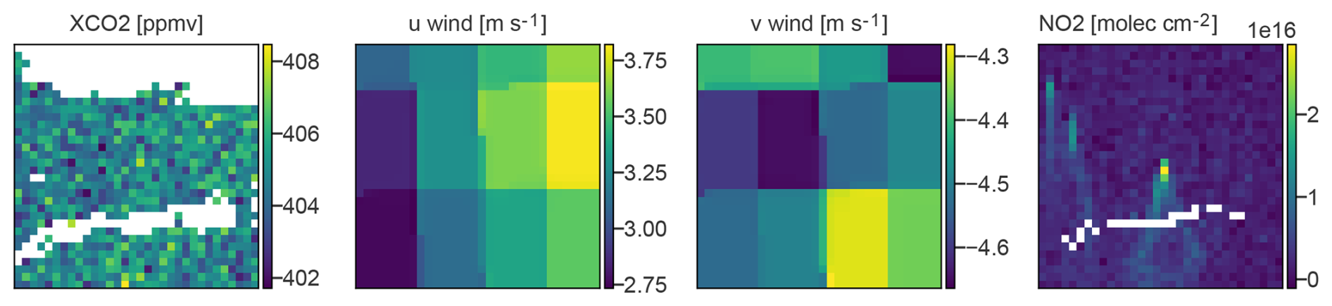
Figure 1 Examples of inputs used by the CNN model. The first, second, third, and fourth columns represent the XCO₂ images, vertically averaged u winds, vertically averaged v winds, and NO₂ images, respectively. The power plant of interest is always located in the middle of the image.

2.2 Set of OCO-3 SAMs

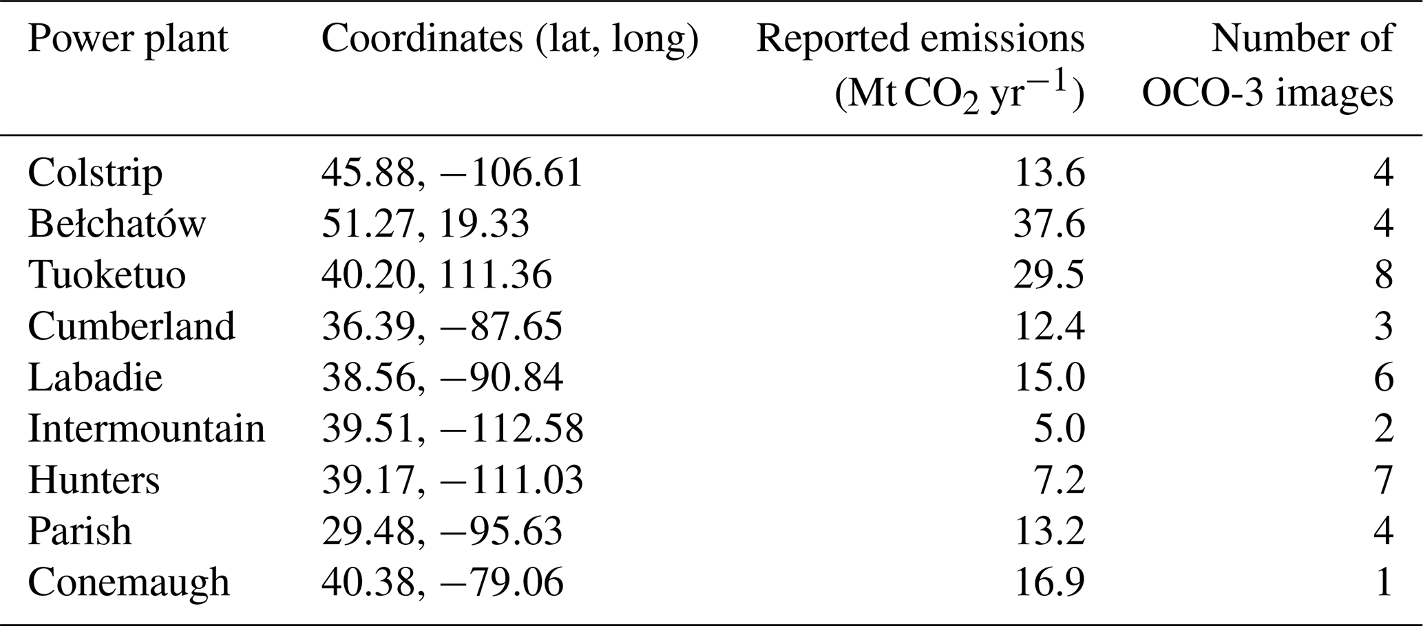
The OCO-3 SAM mode is an observation strategy designed to monitor CO₂ emissions from specific emission hotspots (large urban areas and large industrial point sources). Unlike OCO-3's standard observation mode, which conducts continuous scans of the Earth's atmosphere in nadir or glint mode, the SAM mode is a targeting mode that provides high-resolution XCO₂ images around such emission hotspots. In this study, we selected 39 OCO-3 SAMs at nine power plants to evaluate the applicability and reliability of our CNN model trained on synthetic datasets. We selected OCO-3 SAM images corresponding to (1) power plants for which reports of the emissions are available and have been studied in the scientific literature and (2) a sufficient number of cloud-free XCO₂ retrievals of good quality are available. The list of power plants selected are described, including the average reported emissions and number of collected SAMs, in Table 1.

Table 1 List of power plants selected for this study, along with their annual reported emissions, coordinates, and number of observations used. The data span from 2020 to 2023. Emission statistics are sourced from Nassar et al. (2021), Grant et al. (2021), and Lin et al. (2023), which are based on the US Environmental Protection Agency (EPA, https://www.epa.gov/airmarkets/power-sector-emissions-data, last access: 15 June 2025) and the European Pollutant Release and Transfer Register (E-PRTR, https://www.eea.europa.eu/en, last access: 15 June 2025).

To adapt the raw OCO-3 SAM data for CNN analysis, we first construct a 32 pixel × 32 pixel grid with a resolution of 2 km (similar to the resolution of OCO3 SAMs or CO2M) centred on the power plant. Each grid cell is populated through a weighted interpolation of surrounding OCO-3 SAM data pixel centres, considering only those within a distance of less than 0.66 times the new grid resolution. This specific distance threshold was determined through experimentation to optimally preserve information from the original dataset. Although this mapping strategy provides a straightforward means of converting OCO-3 SAM data into a format compatible with our CNN, it is acknowledged that this approach has limitations and that the observation information might not be perfectly conserved. Additionally, as most OCO3 SAMs used in this study were taken in 2021 or 2022, the synthetic images are adjusted to account for the effect of climate change and the general increase in the CO₂ concentration of 2.3 ppm yr⁻¹ since 2015 (SMARTCARB synthetic dataset year). Using eight examples, Fig. 2 illustrates the process of transforming original OCO-3 SAM data into an XCO₂ field suitable for CNN reconstruction.

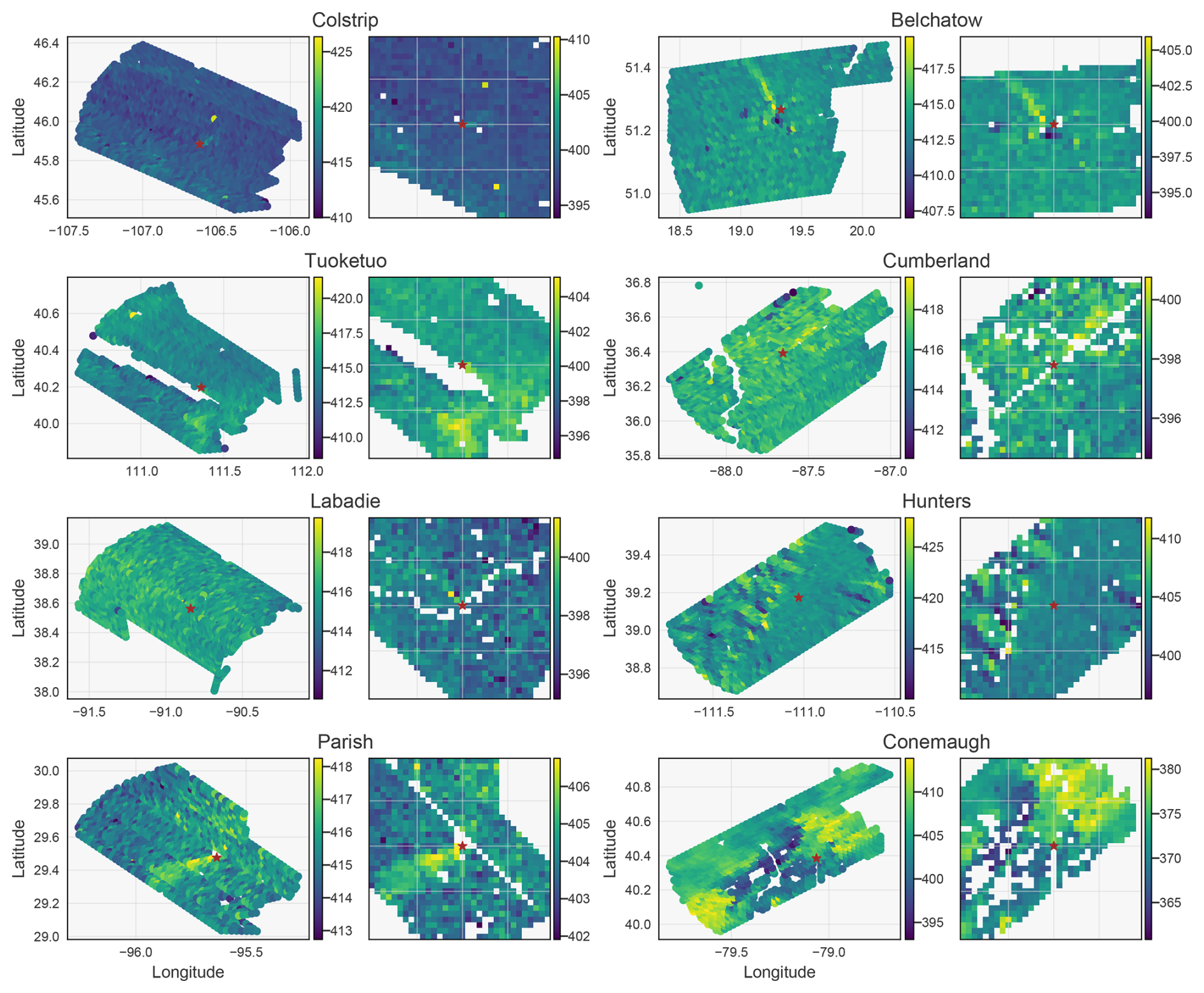
Figure 2 Examples of OCO-3 SAM observations for eight different power plants and the transformation of these observations into CNN-compatible images. For each case, the original OCO-3 SAM data are described on the left, whereas the corresponding CNN-compatible mapping (in which the power plant is always in the centre of the image) is shown on the right. All values are in parts per million by volume (ppmv).

2.3 Training, validation, and test split choices

For tests on synthetic and real data, to avoid data leakage, a rigorous geographical separation is maintained between the power plants used in the training and validation datasets and those used in the test dataset. For instance, when training a model to predict emissions from the Boxberg power plant, Boxberg plumes are excluded from the training set. The validation dataset comprises plumes from a different power plant, Dolna Odra, which is neither used to train nor test the CNNs. This splitting strategy is outlined in Fig. 3.

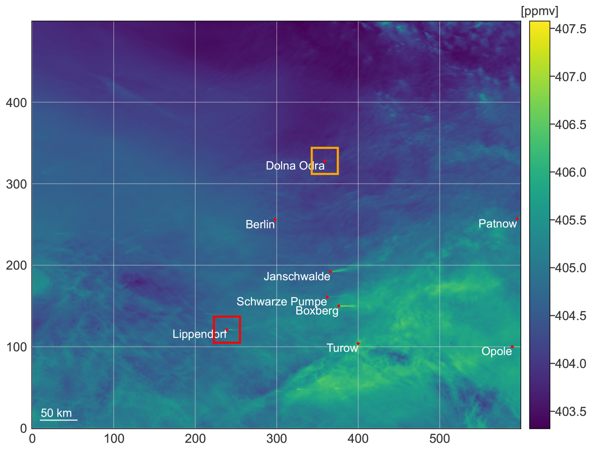
Figure 3 Map of XCO₂ concentrations within the complete SMARTCARB domain on 12 December 2015 at 03:00 UTC. The depicted XCO₂ fields are devoid of synthetic satellite noise for visibility. When constructing a model to predict emissions from Lippendorf, based on Lippendorf-centred fields (indicated by the red square), images from Dolna Odra (indicated by the orange square) are used for validation, whereas images from the remaining power plants serve as training data.

This approach mirrors the strategy adopted in Dumont Le Brazidec et al. (2024a) for the analysis of synthetic images. We focus on the same three power plants for the tests – Lippendorf, Boxberg, and Turów – and train distinct models for each to predict their emissions. These models share the same architectural framework, hyperparameters, CNN structure, and preprocessing layers, but they are trained on a dataset excluding plumes from the target power plant.

The rationale behind selecting Lippendorf, Boxberg, and Turów as test power plants is thoroughly discussed by Dumont Le Brazidec et al. (2024a). Briefly, these power plants were chosen for their distinct characteristics: Lippendorf's average emissions are equal to 15.2 Mt CO₂ yr⁻¹; Boxberg's plume is often located close to other power plant plumes and its average emission amount to 19.0 Mt CO₂ yr⁻¹; and Turów is characterized by low emissions of 8.7 Mt CO₂ yr⁻¹. These selection criteria ensure an evaluation of the proposed CNN architecture across various emission scenarios.

It is critical to underline that while the test dataset for one experiment becomes part of the training dataset for another, each experiment was conducted independently, ensuring that model tuning was not optimized by outcomes derived from the test datasets. Finally, in our assessment of CNNs against OCO-3 SAM data, the training was based exclusively on synthetic data.

3 Deep learning methodology

The goal of this study is to determine the CO₂ emission rate (in MtCO₂ yr⁻¹) of the hotspot in the centre of a XCO₂ image using a CNN model, which takes the XCO₂ image (alongside other data) as input. This section describes the CNN model and the data augmentation strategy, with a particular focus on the method to address cloud interference, and discusses training parameters.

3.1 CNN model and preprocessing layers

This subsection describes the CNN-based inversion system (the CNN model with its preprocessing layers that estimates emissions from images) and how it is trained. The CNN-based inversion system is a compound of preprocessing layers and a core CNN model. Preprocessing layers are operations successively applied to the XCO₂ fields and ancillary data before they are processed by the core CNN model. The core CNN model is a statistical model whose parameters (or neurons) are optimized during the training phase; its function is to identify and extract features from the input data, which it learns to associate with specific levels of emissions. The training phase of the CNN-based inversion system consists of a series of five steps, depicted in Fig. 4 and outlined in the following paragraphs.

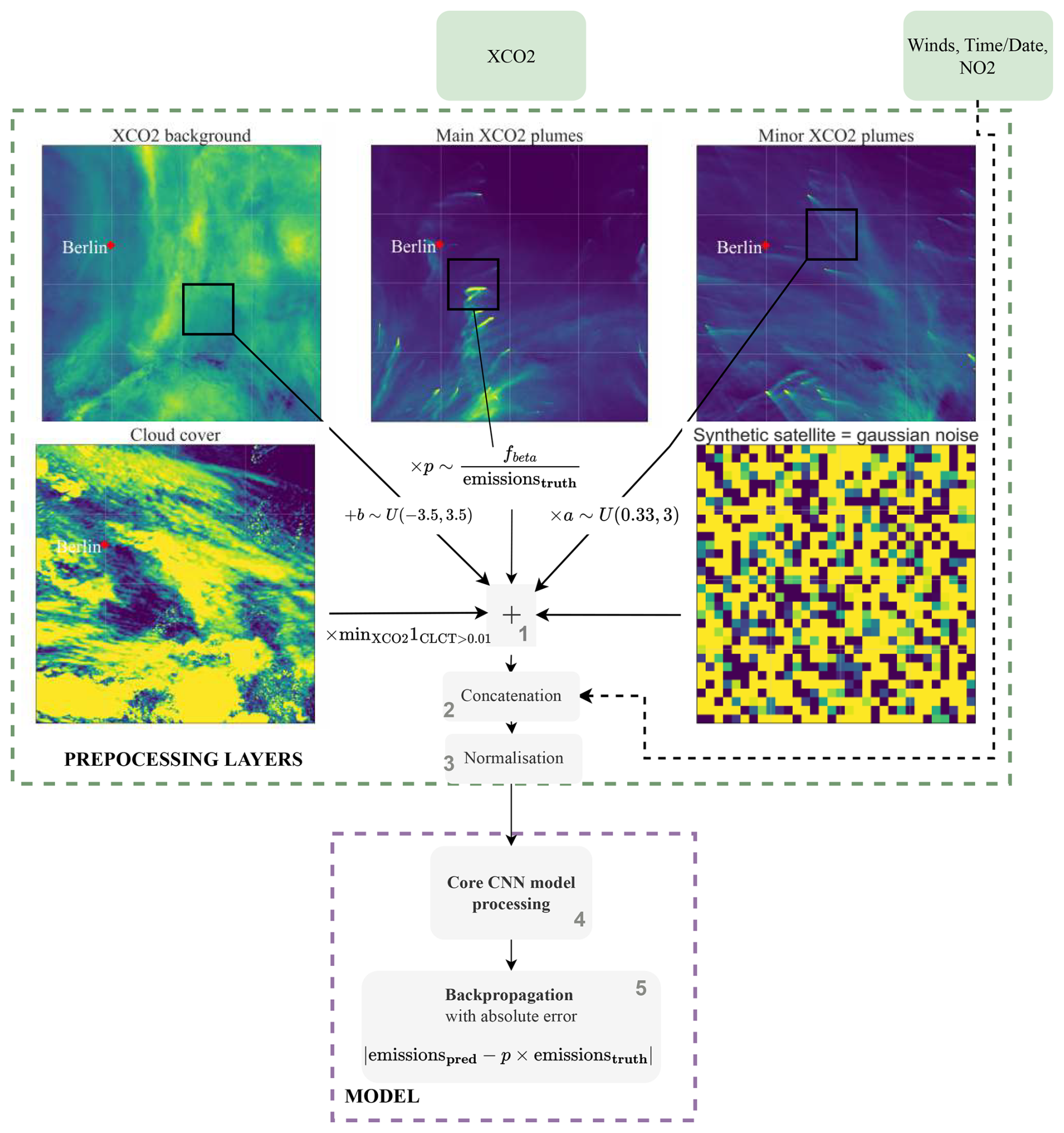
Figure 4 Description of the inversion system at the training time as a compound of preprocessing layers and the model. The CNN-based inversion system consists of five steps. First, in step (1), an XCO₂ field is constructed as the sum of the background XCO₂, major and minor CO₂ plumes, cloud cover, and synthetic satellite noise, with the latter represented by Gaussian noise with a standard deviation of 0.7 ppmv and a 0 mean. The major plumes are scaled using either a beta or uniform distribution (with only the beta distribution shown in the figure), a uniform random field of between −3.5 and 3.5 ppmv is added to the background, and the remaining plumes are scaled by random factors drawn from a uniform distribution of between 0.33 and 3. Pixels in the reconstructed XCO₂ field are marked as missing (NaN) when cloud cover exceeds a specified threshold. The plumes of interest are augmented by a beta or uniform distribution (only beta is represented in the figure), the background is added to uniformly drawn fields of between −3.5 and 3.5 ppmv, and the other plumes are multiplied by a uniform distribution of between 0.33 and 3. The reconstructed XCO₂ field pixels are considered to be NaN or not according to the clouds based on a given threshold. In step (2), concatenation with ancillary data (winds, time, and NO₂) is undertaken. Step (3) involves the standardization of the fields. Step (4) entails processing by the core CNN model. Finally, step (5) involves backpropagation.

3.1.1 Data augmentation

The data augmentation process creates an artificially infinite dataset from the SMARTCARB dataset to prevent the model from overfitting due to the SMARTCARB dataset's limitations. Specifically, instead of using the XCO₂ field directly from the SMARTCARB dataset to train the core model, we use a composition of five different elements:

1. The principal component is a synthetic image centred on a major power plant of interest, exclusively containing the XCO₂ plume from that facility and the other major power plants. The SMARTCARB dataset composition facilitates isolating this field from all other anthropogenic and biogenic fluxes. This first component undergoes a distribution mapping, whereby an emission level is randomly drawn from a probability distribution, either a beta (to mitigate the training on extreme emissions) or a uniform distribution, as shown in Fig. 5, and the plume image is adjusted accordingly (we trained separate CNN models for each distribution choice). Simultaneously, the CNN output is also adjusted at the emission level.

2. A randomly drawn XCO₂ background, which is augmented by summing it with a random number $b\sim U(-\mathrm{3.5},\mathrm{3.5})$ (in ppmv), is added, uniformly across the field, to this first component in a manner analogous to Dumont Le Brazidec et al. (2024a). The selection of the background (and all subsequently described elements) through uniform random drawing is independent of the position of the main plume component.

3. Other anthropogenic XCO₂ plumes identified in the SMARTCARB area, each scaled by a random factor ranging from 0.33 to 3, are added to this.

4. The application of cloud cover constitutes the fourth component. A random selection of cloud cover from the SMARTCARB area is made, independent of the selections for other fields. The XCO₂ pixels are deemed unobserved when cloud cover exceeds 0.01, leading to replacement with NaN, and are subsequently replaced with the minimum value across all XCO₂ fields. This is done in order for the CNN model to learn to ignore this non-informative constant value.

5. The fifth component adds random Gaussian noise with a variance of 0.7 ppmv to the other fields.

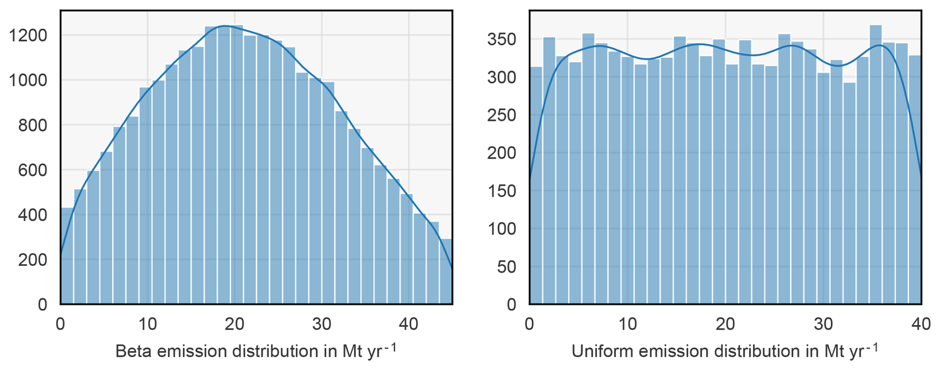
Figure 5 At training time, the hotspot emission and corresponding plume are adjusted based on a random draw from either a beta or uniform distribution.

3.1.2 Concatenation

The concatenation of the main XCO₂ field with the ancillary data represents the second step. The ancillary data may include wind conditions, the time and date of the observation, and the NO₂ field. In instances where the NO₂ field is incorporated, it also undergoes a data augmentation process (not depicted in Fig. 4). Initially, the NO₂ plume is scaled by a random factor drawn from a uniform distribution ranging from 0.75 to 2 to ensure that the NO₂ plume amplitude is decorrelated from that of the CO₂ plume, thereby preventing the core CNN model from relying on the tight correlation between the NO_x and CO₂ emissions for the inversion. In principle, due to the large variations and uncertainties in the CO₂-to-NO_x emission ratios and the lifetime of NO_x, NO₂ should primarily support the plume detection in the overall inversion process. Subsequently, the NO₂ field is partially masked due to cloud cover. For this, we adopt the criterion from Kuhlmann et al. (2019): an NO₂ pixel is marked as NaN if its cloud cover fraction exceeds 0.3. Furthermore, the NO₂ field is subject to Gaussian noise with a variance of 1×10¹⁵ molec. cm⁻² (Kuhlmann et al., 2019).

3.1.3 Normalization

Z-score normalization of each physical field within the concatenated input data constitutes the third step and is performed independently for each channel.

3.1.4 Processing

The fourth step is the core CNN model mapping from XCO₂ and ancillary fields to a scalar emission value. This model, consistent with that described in Dumont Le Brazidec et al. (2024a), features a series of convolutional, max pooling, batch normalization, and dropout layers, with a total of 186 000 trainable parameters. Specifically, if time and date features are used, they are integrated into the CNN following the feature extraction (following the last dense layer).

3.1.5 Backpropagation

The final step entails computing the loss gradient, enabling neuron adjustments within the core CNN model through backpropagation.

In contrast to the training phase, the inversion system in the evaluation phase consists only of the concatenation, normalization, and processing by the core CNN model. The synthetic test dataset consists of preconstructed, physically consistent simulated data (except for clouds, as explained in Sect. 3.2), maintaining consistency with the methodology outlined in Dumont Le Brazidec et al. (2024a).

3.2 Clouds

To assess the impact of cloud cover on CNN performance, we consider models trained and tested on varied datasets distinguished by varying degrees of fraction of cloudy pixels in the XCO₂ images:

• A first series of models are trained and tested on XCO₂ images under clear-sky conditions.

• A second series of models are trained and tested on XCO₂ images with cloud cover ranging from 0 % to 25 %.

• A third series of models are trained on XCO₂ images with cloud cover from 0 % to 50 % but are tested on images with cloud cover from 25 % to 50 %.

• A final series of models are trained on XCO₂ images with cloud cover from 0 % to 75 % but are tested on images with cloud cover from 50 % to 75 %.

These varying degrees of cloud cover are constructed through random sampling of cloud cover over the SMARTCARB domain. This method of training and testing models under varying cloud conditions allows us to compare the degradation of model performance with increased cloud cover. Additionally, training the model tested on cloud cover between 50 % and 75 % on a range from 0 % to 75 % ensures the maintenance of a “universal” model capable of inverting plumes in scenarios with both low and high cloud cover.

3.3 Training parameterization

We configure the training hyperparameters as follows: the model uses the Adam optimizer, with an initial learning rate of $\mathrm{1}\times {\mathrm{10}}^{-\mathrm{3}}$, which is adjusted according to a reduce-on-plateau strategy down to $\mathrm{1}\times {\mathrm{10}}^{-\mathrm{5}}$ with a patience parameter set to 20. The batch size is established at 128, and the training process spans 750 epochs. These parameters were selected based on a rigorous experimental process, combined with adherence to established practices in the field. For the loss function, the mean absolute error (MAE) was chosen.

4 Application to synthetic and OCO-3 SAM observations

4.1 Application to synthetic dataset

Similarly to Dumont Le Brazidec et al. (2024a), we investigate the performance of various CNN models with respect to predicting the emissions of the Lippendorf, Turów, or Boxberg power plants. A collection of CNNs undergo training on subsets of power plants, each excluding one for evaluation. For each power plant, the collection corresponds to models that are trained and tested on images affected by varying levels of cloud cover. In addition, the models are trained with two different input configurations: one that includes XCO₂, wind, time, and NO₂ data and another that includes all of these variables except for NO₂. As a result, a total of 3 (number of target power plants) × 4 (cloud cover scenarios) × 2 (input configurations) = 24 CNNs are trained and evaluated.

Figures 6 and 7 show kernel density estimation (KDE) plots for the absolute relative error and the algebraic difference between the model predictions and the true emissions for the configuration without and with NO₂ input. A comprehensive summary of the results is also provided in Table 2.

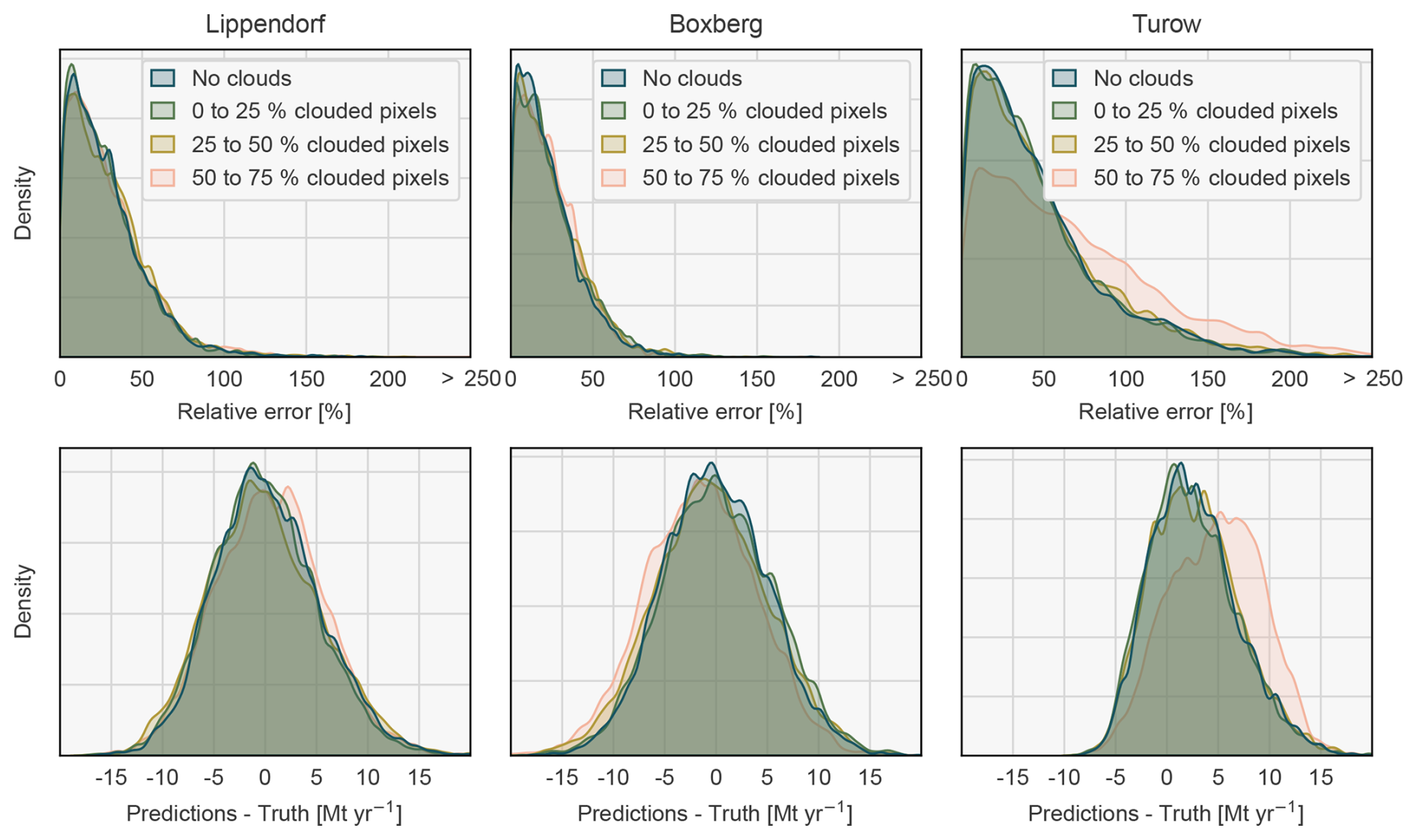
Figure 6 Density plots of the absolute relative error and of the algebraic difference between the CNN predictions and the reported emissions. The CNN models are trained and evaluated with XCO₂, wind, and time input data, affected by varying levels of cloud cover. Predictions with absolute relative errors greater than 250 % or absolute errors greater than 15 Mt yr⁻¹ were set to 250 or 15, respectively, to increase visibility.

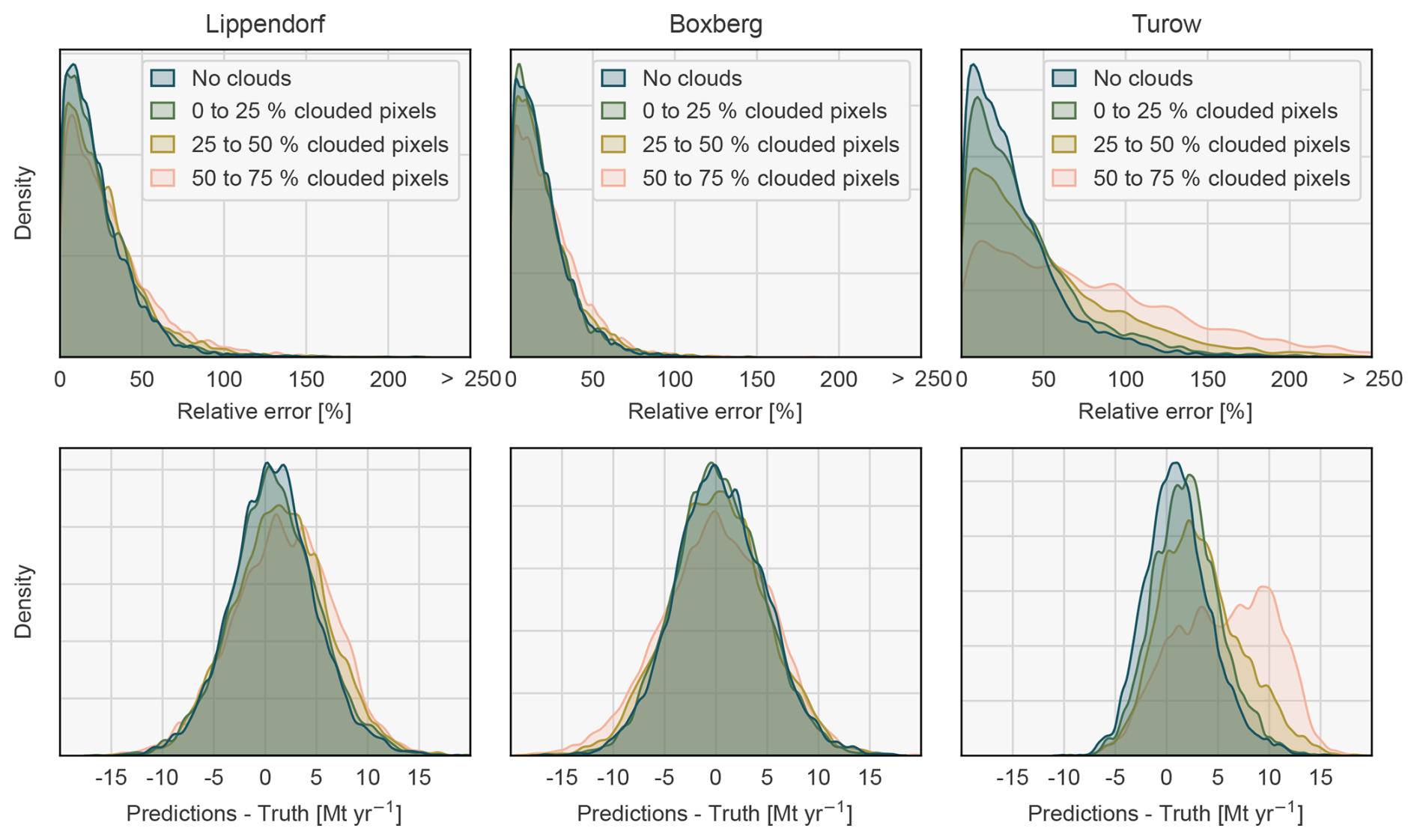
Figure 7 Density plots of the absolute relative error and of the algebraic difference between the CNN predictions and the reported emissions. The CNN models are trained and evaluated with XCO₂, wind, time, and NO₂ input data, affected by varying levels of cloud cover. Predictions with absolute relative errors greater than 250 % or absolute errors greater than 15 Mt yr⁻¹ were set to 250 or 15, respectively, to increase visibility.

Table 2 Median of the relative error between the CNN predictions and the true emissions for Lippendorf, Boxberg, and Turów for varying levels of clouds and input configurations. Entries in the table represent relative errors expressed as percentages of the true emissions.

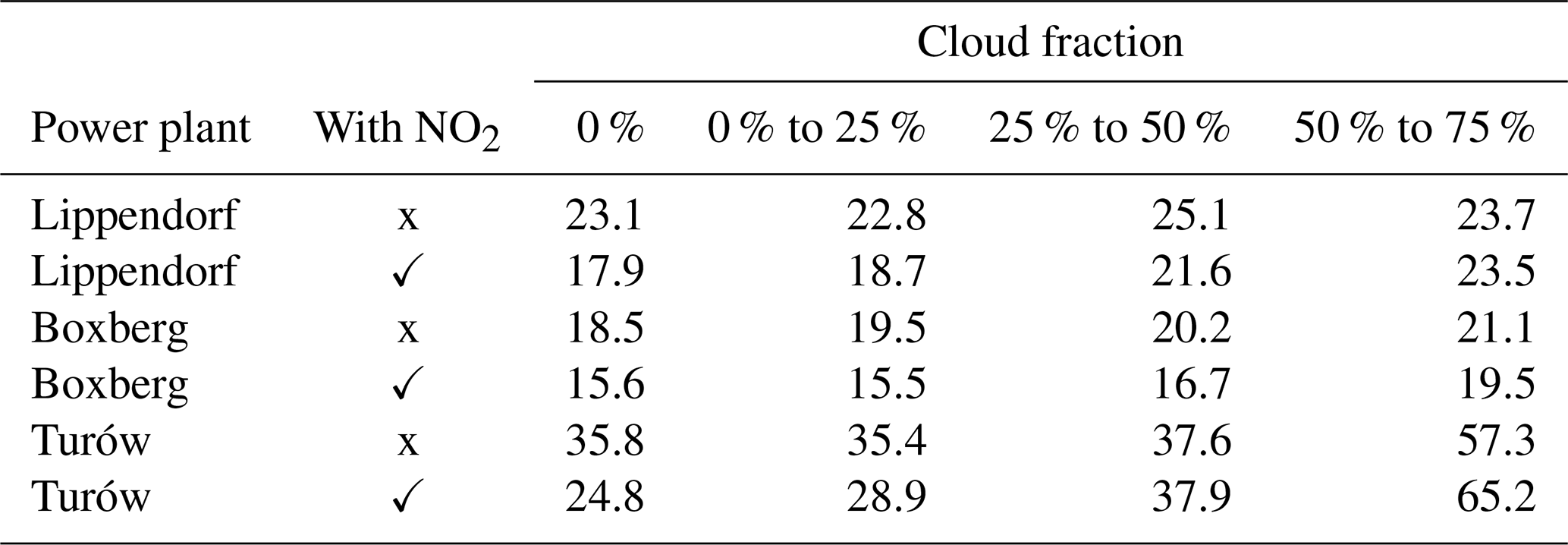
The novel data augmentation strategy presented in Sect. 3.1 improves the stability of the performance of the CNNs in comparison to Dumont Le Brazidec et al. (2024a), making it unnecessary to train a CNN ensemble to achieve satisfactory and consistent results. Significantly, in comparison to Dumont Le Brazidec et al. (2024a), the Boxberg median relative error with NO₂ decreased from 36.9 % to 15.6 %. Furthermore, an improvement in the results is observed when using the mean of the emissions predicted by applying the CNN to an ensemble of images with added Gaussian noise (not shown). Specifically, for added Gaussian noise with a standard deviation of 0.3, the Lippendorf median relative error (without additional inputs) decreases from 23.1 % to 18.5 %. Finally, incorporating time or wind as a feature yields no significant benefit with respect to the performance of the CNNs.

Concerning the influence of clouds, in the cases of Lippendorf and Boxberg, the accuracy of plume emission predictions is not significantly compromised by their introduction, even with a high cloud cover exceeding 50 %. This observation is valid whether or not NO₂ is factored into the analysis. However, for Turów, a power plant with lower emissions, the performance of CNN predictions degrades progressively with an increase in cloud cover, notably when cloud cover exceeds 50 %. The specific decline in prediction accuracy for Turów can likely be traced back to the fact that Turów's plume is mostly indistinguishable from the background. Consequently, the CNN's capacity to accurately estimate Turów's emissions is inherently based on limited information, even in the absence of clouds. The introduction of cloud cover exacerbates this issue by further diminishing the available information.

4.2 Application to OCO-3 SAM observations

In this section, we assess the ability of CNNs trained on power plant plumes from the SMARTCARB synthetic dataset encompassing the power plants of Jänschwalde, Schwarze Pumpe, Boxberg, Lippendorf, Turów, Pa̧tnów, and Opole, to estimate emissions from real plumes observed at power plants by OCO-3 SAM, along with ERA5 wind fields and time information. A total of 39 observations of OCO-3 SAM data for nine power plants are examined.

To obtain meaningful statistics from the small number of images, we use two different methods to increase the number of predictions for each image:

1. an ensemble of 100 images $x_i^{\mathrm{1}},\mathrm{\dots },x_i^{\mathrm{100}}$ for each normalized OCO-3 SAM observation x_i, where $x_i^j\sim \mathcal{N}(x_i,\mathrm{0.3})$;

2. an ensemble of 16 neural networks, all trained with slightly different hyperparameters considering various levels of cloud cover and with either uniform or beta distribution used for augmentation.

Each neural network generates 100 predictions from the 100 images. The ensemble mean should give a more accurate estimate than a single prediction for x_i, as seen with the synthetic data (see Sect. 4.1). Together with the 16 networks, we obtain 1600 predictions for each image, enhancing the robustness and reliability of our statistical analysis.

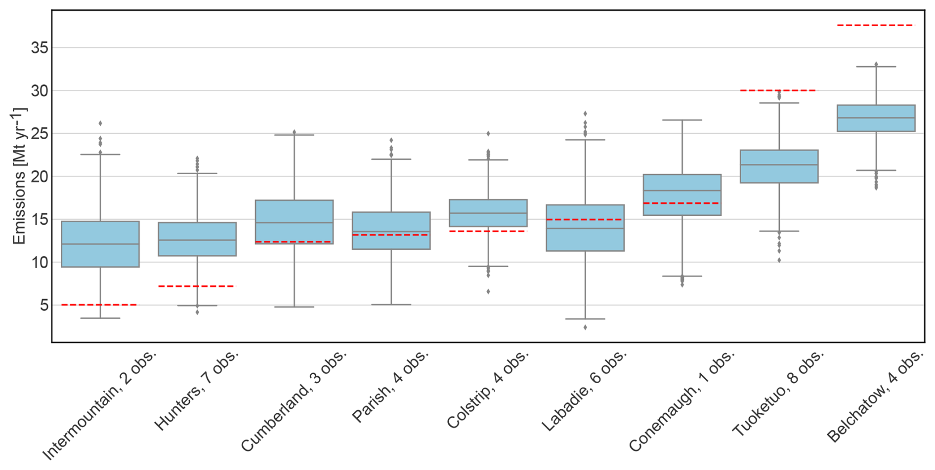
Figure 8 Box plots of the ensembles of predictions based on the OCO-3 SAM observations for various power plants. Comparison with the reported annual emissions of the corresponding power plants (dashed red lines). Boxes span the quartiles (25th to 75th percentiles), whiskers extend to the last points within 1.5 × IQR (interquartile range), and points beyond the whiskers represent outliers

Figure 8 shows the ensemble of predictions for each power plant compared to the annual reported emissions. The median absolute and median absolute relative differences between the ensemble average predictions and the reported emissions are 7 Mt yr⁻¹ and 29 %, respectively. This relative difference of 29 % is only slightly higher than what was observed on synthetic satellite imagery. Specifically, CNNs exhibit a good match with reported emissions for power plants with emissions ranging between 10 and 20 Mt yr⁻¹ (e.g. Colstrip, Cumberland, Labadie, Parish, and Conemaugh). However, the discrepancy with reported emissions largely increases for power plants at the extremes of low or high emissions (e.g. Bełchatów, Tuoketuo, Hunters, and Intermountain). The emissions estimated by the CNNs range from 6.7 to 30.4 Mt yr⁻¹ (considering the 5 % and 95 % quantile predictions), whereas Bełchatów's reported emissions stand at 37.6 Mt yr⁻¹ and Intermountain's stand at 5 Mt yr⁻¹. This indicates that the variance in CNN predictions is significantly lower than that of the reported emissions. Given that the CNNs were trained on plumes with emission levels spanning from 0 to 45 Mt yr⁻¹, it was initially anticipated that they could accurately predict plumes akin to those from Bełchatów or Intermountain. Furthermore, in Sect. 4.1, we show that the CNNs reliably recover the low emissions (8.7 Mt yr⁻¹ on average) of the Turów power plant. The subsequent analyses will explore the causes of the observed discrepancies between extreme reported emissions and CNN predictions.

Figure 9 shows the predictions of a randomly selected CNN model from the ensemble for eight specific OCO-3 SAM images. These images were chosen after a thorough inspection of all 39 snapshots in our dataset to illustrate the key patterns that we identified. For each OCO-3 SAM image, we show a sensitivity map obtained by the integrated-gradient method, which computes the gradient of the model's output (the emissions) relative to its input pixels, indicating how emissions are expected to increase or decrease with changes in pixel values (see Dumont Le Brazidec et al., 2024a, for details). Assuming that emission estimates are directly correlated with the detection of plume pixels, the integrated-gradient maps are anticipated to highlight a collection of positive pixels that effectively reconstruct the plume.

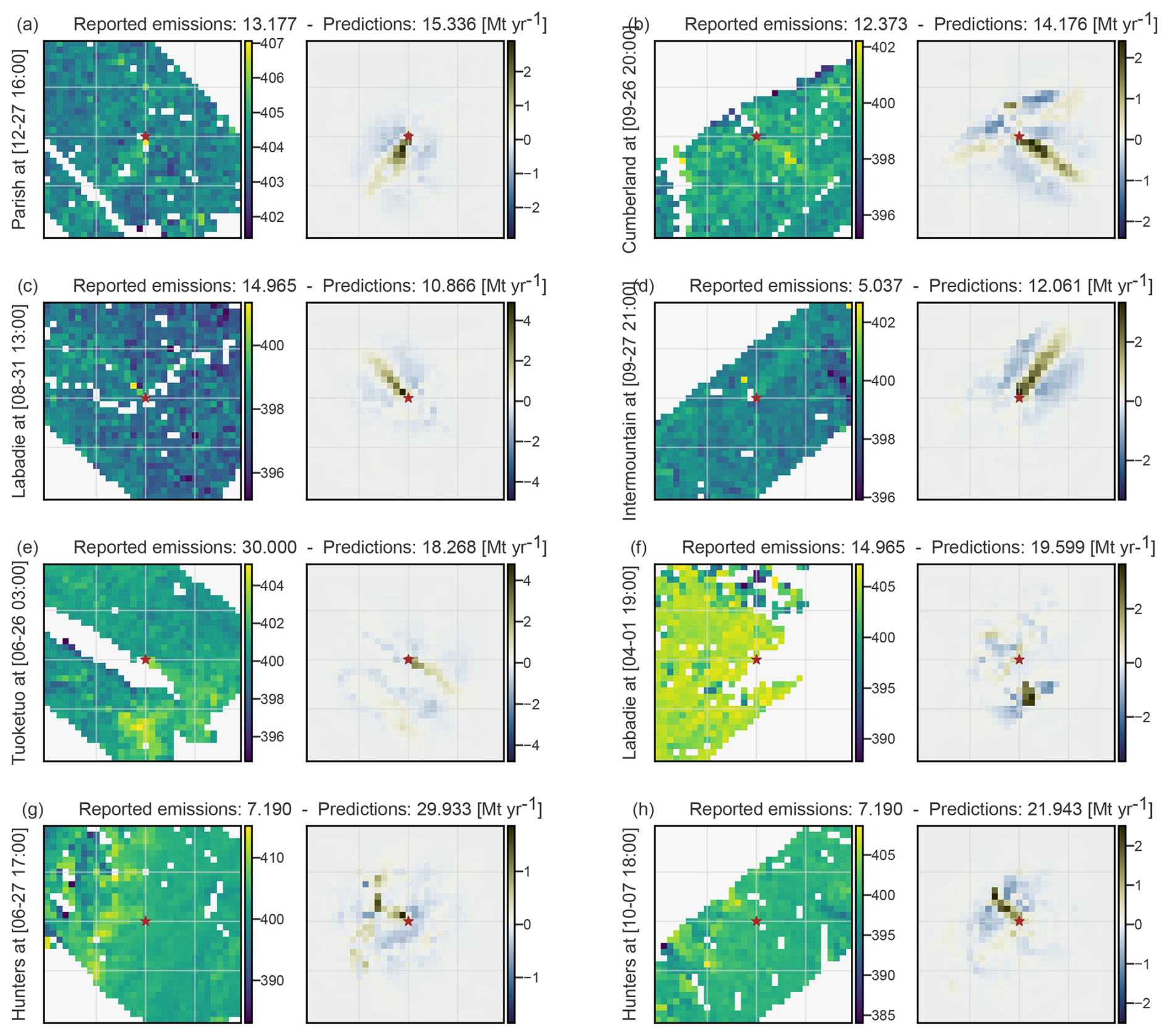
Figure 9 Analysis of the predictions of a CNN (chosen randomly from the ensemble) on eight specific OCO-3 SAM images. Each of the images is presented alongside the resulting map (on its right) from the application of the integrated-gradient method and the reported and predicted emissions in megatonnes per year (Mt yr⁻¹). The power plant is indicated by a brown star. The CO₂ concentration fields on the left are shown in parts per million by volume (ppmv). The integrated-gradient images on the right represent dimensionless scores that indicate the contribution of each pixel to the predicted concentration.

Figure 9a, b, c, and d are four instances of clear identification of the plume by the CNN. The integrated-gradient method in each of these cases reveals collections of positive pixels forming a discernible plume shape. These positive pixels are encircled by negatives, suggesting that if the surrounding pixels intensified to match the plume's pixel values, the CNN would be less likely to recognize these as plume pixels, interpreting the aggregate as elevated background values instead. Predictions closely match reported emissions in each scenario, barring the anomaly of Intermountain. This discrepancy is logical, given that the Intermountain plume is visually detectable in the image, whereas plumes corresponding to emissions of 5 Mt yr⁻¹ in the SMARTCARB dataset are typically obscured by the background.

Figure 9e and f illustrate scenarios where clouds obscure the central portion of the image, thereby concealing a major part of the plume. These examples allow us to investigate how the CNN adapts to such conditions, making inferences based on the limited information available. In Fig. 9e, the CNN identifies a plume adjacent to the obscured area and bases its emission estimate on this collection of pixels. In Fig. 9g, the CNN interprets a significant cluster of high-value pixels as the tail end of the concealed plume and calculates emissions based on this inferred section of the plume.

Figure 9g and h shed light on a primary cause of the supposed overestimation of emissions from low-emission power plants. These images feature barely discernible plumes alongside significant patterns (potentially systematic satellite errors) appearing on the left side of the images in both cases. The CNN mistakenly identifies these patterns as part of a plume in each case. Consequently, the model infers disproportionately high emissions based on this noise, leading to a substantial overestimation of the emissions of these power plants.

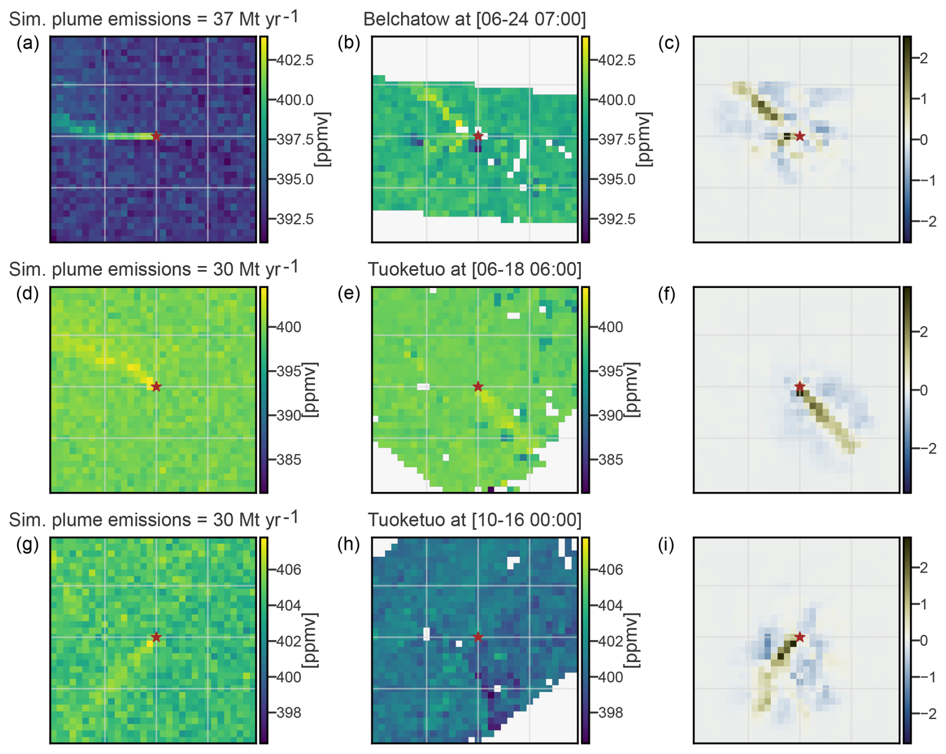
Figure 10 Analysis of the predictions of a CNN (chosen randomly from the ensemble) for three high-emission plumes. One plume from Bełchatów and two from Tuoketuo (b, e, h) are compared against equivalent high-emission plumes from the SMARTCARB dataset (a, d, g). For each OCO-3-SAM-based plume, the integrated-gradient approach is applied and presented in panels (c), (f), and (i). To ensure a fair comparison between columns 1 and 2, identical colour bars have been used. Power plants are indicated by a brown star.

In Fig. 10, we propose a first possible explanation for the underestimation of high-emission plumes by the CNN. Three observed high-emission plumes – one from Bełchatów and two from Tuoketuo – are compared against SMARTCARB plumes at the Bełchatów- or Tuoketuo-reported emission levels. Specifically, the SMARTCARB simulations are chosen to represent emissions of 37 and 29.5 Mt yr⁻¹, aligning with the reported emissions for Bełchatów and Tuoketuo, respectively, and have comparable ERA5 wind speeds to those of the Bełchatów or Tuoketuo snapshot OCO3 SAM images. The simulated plumes appear more pronounced against the background than their real counterparts, suggesting a higher emission magnitude. This observation might account for the model's tendency to estimate lower emissions than Bełchatów- and Tuoketuo-reported emissions. Further validation comes from the integrated-gradient analysis, indicating accurate plume contour predictions by the model and affirming that the relevant information was used for its estimations.

Another reason for the CNN underestimating high-emission plumes could be regression towards the mean in scenarios with high cloud levels. To show this, we train a CNN with a dataset of power plants with uniformly distributed emissions between 0 and 40 Mt yr⁻¹ and a low cloud cover (<25 % of the image covered with clouds). In Fig. 10, we plot the distribution of the predictions of the CNN for synthetic images of the Dolna Odra power plant with uniformly distributed emissions against the truth at different levels of cloud cover.

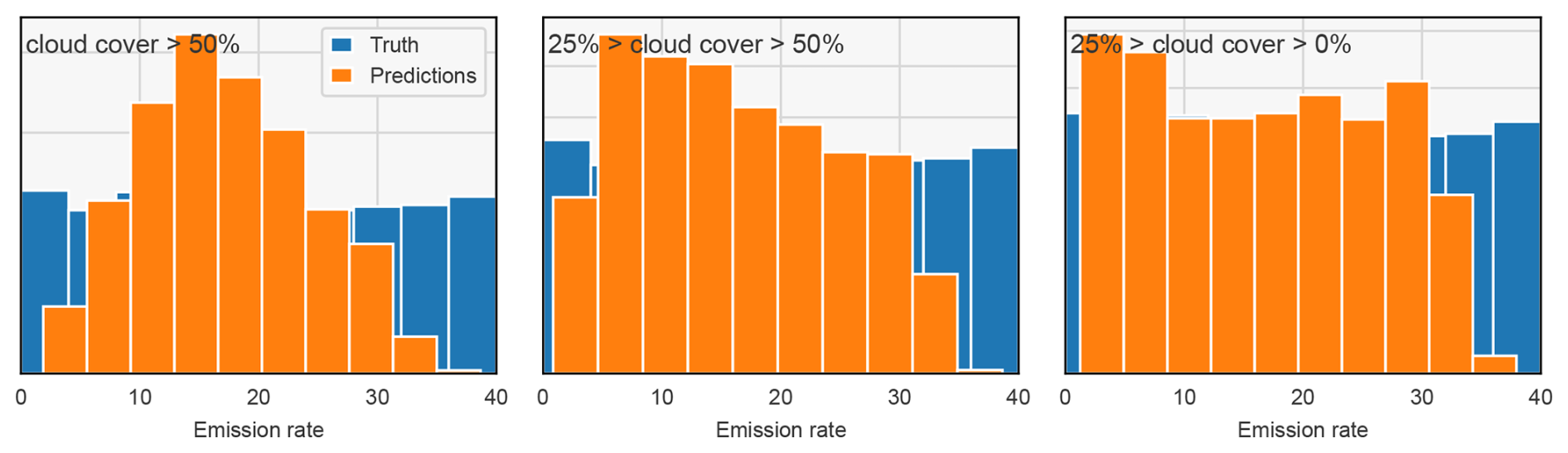
Figure 11 Distribution of the predictions of a CNN trained with uniformly distributed emissions for synthetic images of the Dolna Odra power plant with uniformly distributed emissions against the truth at different levels of cloud cover.

We observe a convergence to average values correlated with cloud cover intensity. When the CNN lacks sufficient information in the image to infer emissions, it tends to average its predictions to minimize loss. A second observation is that, even for low cloud cover, the CNN struggles with emission levels higher than 33 Mt yr⁻¹, while it is trained with emissions uniformly distributed between 0 and 40 Mt yr⁻¹ (note that the CNNs trained in previous sections were trained for emission levels between 0 and 45 Mt yr⁻¹). Increasing the number of high-emission plumes in the training dataset would likely reduce the CNN's bias towards emissions near the upper limit defined in the training data.

5 Discussions and limitations

The ability of CNNs to estimate CO₂ emissions from power plant plumes was validated on synthetic satellite images. The presence of cloud cover does not significantly affect the CNNs performance, except in instances of substantial cloud presence. CNNs demonstrate adaptability, leveraging residual information to accurately estimate emissions under heavily clouded conditions. The inclusion of NO₂ data proves slightly beneficial, enhancing the CNN efficacy under all-sky conditions.

Once trained on simulated XCO₂ images, the CNNs can be directly applied to real-world data with high accuracy, unlike traditional methods, which struggle to detect plumes and distinguish them from the background due to the low signal-to-noise ratio of CO₂ plumes. Nevertheless, it is observed that the spread of the CNN predictions is lower than the spread of the OCO3-SAM-reported emissions. Predictions are significantly higher for low-emission power plants, due to the presence of systematic errors in the image that are falsely identified as plumes, and significantly lower for high-emission power plants. Furthermore, predictions are lower than the reported annual emissions for high-emission power plants. This is likely due to regression towards the mean in weakly informative images and/or discrepancies between the training and evaluation datasets. Finally, it is acknowledged that comparing instantaneous emissions measured during satellite overpasses with reports of annual average emissions from the EPA and E-PRTR inventories presents challenges, owing to the variability and intermittent nature of power production and CO₂ emissions.

The divergence between the distributions of real XCO₂ observations and those of the simulations observed in Sect. 4.2, particularly in terms of systematic satellite errors, creates a domain shift between training and test conditions that likely leads to systematic errors in CNN predictions, necessitating CNN adaptation. To account for systematic satellite errors, a promising approach involves mingling real and simulated data during the training phase, such as overlaying a simulated plume of known emissions onto a real background. This method would introduce systematic errors typical of real satellite data while maintaining a controlled environment for supervised learning.

6 Conclusions and perspectives

In this paper, we improve the CNN model for the inversion of CO₂ plumes from Dumont Le Brazidec et al. (2024a) through the introduction of a novel data augmentation strategy and a dedicated approach to deal with clouds. This methodology was validated using the synthetic CO2M observations from the SMARTCARB dataset, demonstrating its efficacy in handling cloud-covered scenarios. Our findings indicate that, on average, clouds do not pose a significant challenge for CNNs, which maintain high performance levels under both sparse- and dense-cloud conditions. An exception is observed in the case of the Turów power plant, where performance significantly drops. This decline is likely attributable to Turów's relatively low emission levels, which result in its plumes being inherently less distinguishable from the background.

Following its validation, the methodology is applied to OCO-3 SAM observations. In total, 39 observations across nine power plants, adjusted for resolution and shape to match CNN input requirements, are analysed. For each observation, an ensemble of predictions is produced by CNNs trained on the SMARTCARB synthetic dataset. The results are promising, exhibiting a relative difference with the reported emissions only slightly superior to the relative error observed with the synthetic dataset. Specifically, predicted emissions for images from power plants with mid-level emissions, such as Colstrip and Parish, correspond very accurately to reported emissions. Moreover, through the application of integrated-gradient techniques, it is demonstrated that the CNNs effectively identify plumes in the OCO-3 SAM images and accurately estimate emissions from the plumes' physical locations.

However, we observed that images capturing low- and high-emission power plants' plumes are prone to overestimation and underestimation, respectively, in comparison to the reported emissions. Systematic satellite retrieval errors are identified as a frequent cause of overestimation in the images of low-emission power plants. These errors, often non-Gaussian and absent in the synthetic training dataset, lead to significant inaccuracies.

This study demonstrates the feasibility of applying neural networks to real satellite imagery of XCO₂ following training on simulated datasets. Although we advocate for the integration of a hybrid training approach that incorporates both real and simulated images in order to improve the robustness and accuracy of the model, we provide a ready-to-use CNN CO₂ plume inversion tool based on satellite imagery.