Improving winter condition simulations in SURFEX-TEB v9.0 with a multi-layer snow model and ice

In winter, snow- and ice-covered artificial surfaces are important aspects of the urban climate and trigger road maintenance operations. Urban climate and road weather models have specialized in simulating these conditions in cities or in the countryside, respectively. In this study, we intend to bridge the gap between road weather models and urban climate models in terms of cold region urban modelling and artificial surface condition predictions in any environment. We have refined the modelling of road surface processes related to winter conditions in the Town Energy Balance (TEB), an urban climate model designed for complex environments. We have developed an ice content prediction to account for the freezing and melting of the water content on the surface. Additionally, we have enhanced the TEB representation of snow on road, moving from a single-layer snow model (1-L), to a more precise multi-layer snow model known as Explicit Snow (ES). We have isolated the winter surface processes from other physical interactions by limiting the evaluation of the experiments to open environments. The experiments are carried out at two locations: the Col de Porte in the Alps and a road weather station in southern Finland. Our findings show that the enhanced TEB model (named TEB-ES) outperforms TEB, as well as a benchmark model, ISBA-Route/CROCUS, but with mixed results against a multiple linear regression in-sample algorithm. For roads with high traffic and/or winter maintenance operations, future modelling work should focus on the representation of anthropic effects.

1 Introduction

There are significant interconnections between urban climate and winter conditions. As in summer, high-density building distribution can induce a pronounced urban heat island effect (UHI). Few studies tried to study its extent and unveil its drivers. For instance, Malevich and Klink (2011) measured, during winter 2008–2009, an average winter UHI of 1 °C in Minneapolis. In Alaska, in a small settlement of 4600 residents, an average 2.2 °C winter UHI was measured (Hinkel et al., 2003). In a typical Arctic city, Varentsov et al. (2018) measured an average UHI of 1.9 °C with extremes up to 11 °C in Apatity city centre. Hinkel et al. (2003), Varentsov et al. (2018), and Bohnenstengel et al. (2014) agree to say that the anthropogenic heat, released mainly from house heating, is strongly correlated with the UHI magnitude. But its relative impact with other potential drivers on the UHI magnitude is still unclear and there is a need for further studies. The snow cover, which can hold for months on artificial surfaces after some large snowfall, may play an important role in this phenomenon. A few studies based on simulations have shown that the presence of snow cover decreased the surface air temperature (Mori and Sato, 2015; Shui et al., 2016), whereas Malevich and Klink (2011) showed an increased UHI. It is clear that specific events of cold conditions such as snowfall and freezing temperatures have a considerable influence on the city climate (Karsisto et al., 2016). Also, the city climate may have a feedback effect on winter conditions, as some evidence suggests that the urban heat island decreases the amount of snowfall and increases the amount of rainfall (Liu et al., 2024).

The presence of a layer of ice or snow insulates the artificial surfaces from the atmosphere by covering significant parts of the city surface. Therefore, covered artificial surface temperatures evolve by conduction. The soil–atmosphere interaction is driven by the changing properties of the ageing snow, instead of the artificial surface materials. Lemonsu et al. (2008) have shown that snow-covered urban surfaces contribute to changes in sensible and latent heat fluxes. The snow layer stores the incoming energy, modifies the surface output fluxes, and releases energy by melting snow or by sensible and latent heat fluxes (Shui et al., 2019). The net surface radiation seems to be greatly impacted due to the high albedo of the snow (Karsisto et al., 2016). Depending on the characteristics of the snow, the incoming energy from the atmosphere can be stored or released as heat flux or melting snow, as measured in the China case study of Shui et al. (2019). In addition, the ice and snow cover acts as a water reservoir. It delays precipitation runoff and drives urban hydrology (Eimers and McDonald, 2015). These conditions lead to concrete impacts on human activities because of the slippery nature of frozen water. They increase the risk of accidents for drivers, pedestrians, and bicyclists. According to Michaelides et al. (2014), the risk of accidents on icy and slippery roads is 2–3 times higher than on dry roads. In Sweden, Andersson and Chapman (2010) showed that accidents were more frequent under winter conditions with a road surface temperature below −3 °C and snow-covered or icy roads. Remote areas are the most vulnerable, and even light snowfall can have serious consequences in countries not accustomed to these conditions (Vajda et al., 2013). Accurate simulations of the winter conditions on artificial surfaces can help to increase our knowledge of cold urban conditions and increase the safety of artificial surfaces used by citizens.

Simulation tools are needed to simultaneously represent the specific properties of urban environments as a coupling of human activities with the specific processes associated with cold conditions. Land surface models (LSMs) based on the physical heat-balance equation are well suited as they can represent various surface types ranging from natural to artificial surfaces in urban environments. Mainly used to provide boundary conditions for atmospheric models, LSMs are key for the prediction of soil–atmosphere fluxes. Several LSMs have been developed specifically for urban environments: the urban climate models.

In urban environments, specific physical processes are needed to represent the town energetics (Masson, 2000). Simple building-averaged models are able to compute radiative trapping, surface energy budgets, and wind channelling (Masson, 2000). They have demonstrated the ability to simulate the urban heat island in summer driven by urban morphology and the capacity of artificial materials to store energy, e.g. the Town Energy Balance (TEB) model (Suher-Carthy et al., 2023). In comparison, the modelling of urban winter conditions has been less studied in the urban climate community (Pigeon et al., 2008). Lemonsu et al. (2010) showed that coupling the road with a simple one-layer snow model (1-L) in an urban climate model (TEB) leads to improved fluxes in winter. The SUEWS (Järvi et al., 2014), TEB (Masson, 2000), and Lodz-SUEB (Fortuniak, 2003) models include a one-layer snow model to take the effect of snow into account during wintertime. CLMU (Oleson et al., 2010) and JULES (Best et al., 2011) go further and include a multi-layer snow model on the road. Karsisto et al. (2016) compared TEB, SUEWS, and CLM at two Helsinki sites and showed that the snow-covered ground fraction plays a major role in winter and spring for the model flux performance. More studies are needed to model and compare the winter conditions with the observations, in particular, the key processes driving the urban response at the surface: snow cover evolution, ice layer evolution, and human activities. To that extent, road weather models are also well suited to simulate the artificial surface response to winter conditions. Many national weather services run land surface models specifically designed to help road winter maintenance. These so-called road weather models focus on integrating various factors that affect the evolution of road conditions (Qin et al., 2022), including the difficult winter road conditions related to snow and ice.

The Canadian road weather model METRo (Crevier and Delage, 2001) and the Norwegian model NORTRIP (Denby et al., 2013; Nuijten, 2016) predict slippery road conditions with a single shared ice/snow storage content. In Finland, RoadSurf (Kangas et al., 2015) computes two distinct snow and ice reservoirs with a simple approach to the melting of ice and snow on the road. The melting energy is taken into account by using the excess energy to melt the ice and snow instead of warming the road when temperature is above the melting point. The Dutch road weather model takes into account freezing and melting energy (Karsisto et al., 2017). Chen et al. (2023) developed a complex formulation for road ice prediction. It computes an explicit one-layer water/ice energy equation with complex heat exchanges between the road and the atmosphere. In France, a modified version of the ISBA hydrological model coupled with two multi-layer snow models (CROCUS and Explicit Snow (ES)) was built for road maintenance purposes (Bouilloud and Martin, 2006; Boone and Etchevers, 2001). ES and CROCUS compute prognostic heat contents, water contents, and densities and have been validated at many alpine sites. The use of CROCUS within ISBA-Route leads to accurate simulations of road conditions on snow-covered roads (Bouilloud and Martin, 2006).

This study attempts to bridge a gap between urban climate models and road weather models used for road maintenance: on the one hand, as they focus on soil–atmosphere heat exchange, urban climate models do not include processes relevant to winter road maintenance. On the other hand, road weather models, with physics comparable to one-tile urban models (Lipson et al., 2024) struggle to compute accurate urban conditions. Some urban climate models bridge part of the gap by including snow (Lemonsu et al., 2010) and ice accumulation in the road component (Meng, 2017). There are also road weather models that take into account sky-view factors and radiation trapping (Karsisto and Horttanainen, 2023; Denby et al., 2013). The aim of this study is to improve the representation of winter processes in the TEB urban climate model. A new version of TEB (TEB-ES) has been developed. It models the challenging winter artificial surface conditions associated with snow and ice. Our work presents a new ice storage term and an improved snow model with a multi-layer parameterization (ES) of snow over the road surface.

Section 2 of the paper first describes the TEB initial version (simply TEB) and then the new processes added in the new version of the model (TEB-ES). Section 3 presents the experimental set-up to evaluate the models' performances in winter conditions. In Sects. 4 and 5, we present the performance of TEB and the TEB-ES model against measurements at two sites, Col de Porte in France and a road weather station in southern Finland. Section 6 comments on the findings of this study and the limitations of TEB-ES in representing winter conditions on artificial surfaces subject to anthropic impacts. Finally, we conclude this study (Sect. 7).

2 Methods

2.1 Initial TEB model

The Town Energy Balance (TEB) model (Masson, 2000) is embedded in the SURFEX software (SURface EXternalisée). The idea in this system was to build a modular system disconnected from an atmospheric model. Rather than being tied to a single atmospheric model, SURFEX can be launched autonomously or coupled to any atmospheric model to provide surface state variables. SURFEX consists of four submodels that describe different surface types on the globe with TEB appropriate to simulate urban environments. Extensively used to study the urban heat island (UHI) in summer, TEB has been validated and incorporated into the Meso-NH model (Lac et al., 2018). Pigeon et al. (2008) performed a winter evaluation of the model in the 2004–2005 Capitoul campaign and showed that the model accurately simulates surface temperature in cases without snow. Lemonsu et al. (2010) evaluated the one-layer snow model coupled with the road and the roof snow during the Montreal campaign.

TEB is a heat-balance model with a local canyon geometry that represents a simplified urban environment. It models two facing walls separated by a road, as first proposed by Oke (1987), which leads to a fast computation. The TEB model solves distinct heat equations for each surface (roof, wall, and road). The radiative trapping inside the canyon geometry leads to specific shortwave and longwave energy balance equations forced by the atmosphere for each surface. The net longwave radiation absorbed by each surface is computed between an interaction with each TEB component. The direct solar flux received by the road or the walls is computed according to shadowing effects and the direction of the road. The diffuse solar flux is processed using a sky-view factor and a geometric system for an infinite number of reflections. The following description of TEB is restricted to its road component, schematically displayed in Fig. 1, as it is the focus of our study. Depending on the TEB configuration during simulations, the road component can represent, simultaneously, roads, sidewalks, and car park.

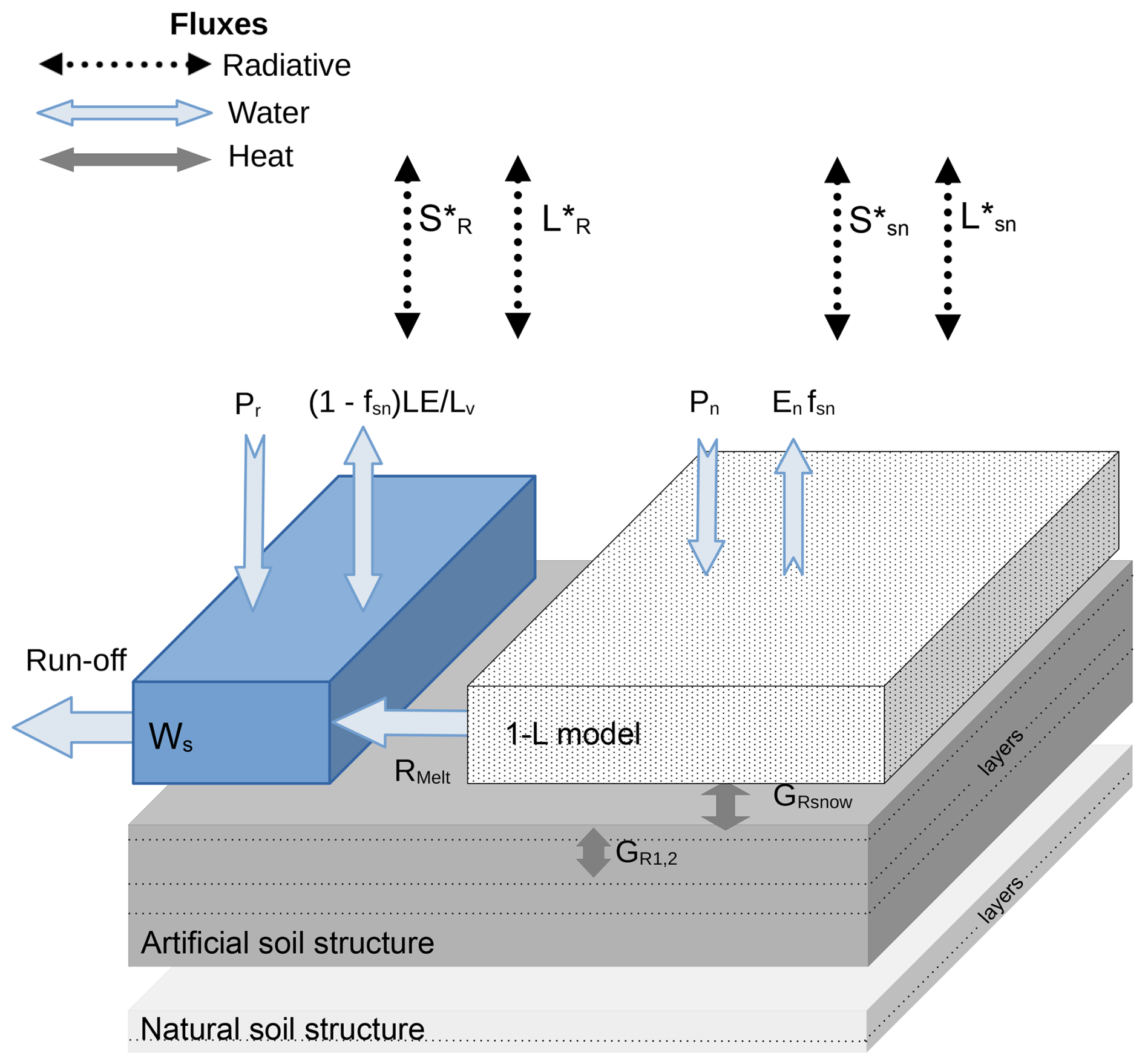
Figure 1 Schematic implementation of the road component in TEB initial version with the 1-L snow model in white, the water content W_s in blue, and their interaction with the road surface in grey. Heat, water, and radiation effects are represented by arrows with radiative fluxes $S_{\text{sn}}^{*}$ and $L_{\text{sn}}^{*}$ (net shortwave and net longwave over snow, respectively).

The ground is discretized with layers of artificial ground representing the road structure and layers of natural soil beneath them. The temperature evolution across all layers is driven by a heat equation that computes the energy stored or emitted depending on weather conditions. The road is assumed to be impermeable, so there is no water drainage within the vertical road layers. The snow and rain intercepted by the soil are confined to the road surface. The snow cover defined as a fraction of the total road surface f_sn partitions the road surface. The snow-covered fraction f_sn is computed from the total snow water equivalent W_snow (kg m⁻²) and the parameter W_snowmax, set to 1 kg m⁻² (Masson, 2000), as

$$\begin{array}{}\text{(1)}& f_{\text{sn}}=W_{\text{snow}}/(W_{\text{snow}}+W_{\text{snowmax}}).\end{array}$$

The snow cover fraction f_sn that depends on the snow water content is included in the heat-balance equation as

$$\begin{array}{ll}{\displaystyle }{C}_{\mathrm{R}\mathrm{1}}{\displaystyle \frac{\partial T_{\text{road}}}{\partial t}}& {\displaystyle }=(\mathrm{1}-f_{\text{sn}}){\displaystyle \frac{\mathrm{1}}{d_{\mathrm{R}\mathrm{1}}}}(S_{\mathrm{R}}^{*}+L_{\mathrm{R}}^{*}-H_{\mathrm{R}}-{\text{LE}}_{\mathrm{R}}-G_{\mathrm{R}\mathrm{1},\mathrm{2}})\\ \text{(2)}& {\displaystyle }& {\displaystyle }+f_{\text{sn}}{\displaystyle \frac{\mathrm{1}}{d_{\mathrm{R}\mathrm{1}}}}(G_{\text{Rsnow}}-G_{\mathrm{R}\mathrm{1},\mathrm{2}}),\end{array}$$

where T_road is the road surface temperature driven by the snow–road conduction flux G_Rsnow, the conduction flux between the first and second road layers G_R1,2, net radiation fluxes $S_{\mathrm{R}}^{*}$ and $L_{\mathrm{R}}^{*}$, shown in Fig. 1, and sensible and latent heat fluxes H_R and LE_R. C_R1 is the heat capacity of the road surface depending on the dry surface heat capacity and of the mass content amount, and d_R1 is the depth of the first road layer with values as described in Table 1.

Table 1 Road configuration and parameters in TEB and the modified model TEB-ES.

According to Eq. (2) the TEB road surface energy budget is divided according to the snow fraction. Indeed, snow cover insulates the road surface from the first canyon air layer and vice versa. The snow-covered road surface budget is only driven by the snow–road conduction term (second right-hand term in Eq. 2). The energy budget on the snow-free fraction of the road is driven by the latent and sensible turbulent fluxes between the road and the interface canyon air layer, by the radiation absorbed by the road, and by the heat conduction from the road sublayers (first right-hand term in Eq. 2).

The rain is intercepted by the snow-free fraction of the road, and transferred into the available water reservoir at the road surface W_s (kg m⁻²). Its maximum capacity W_smax in the snow-free fraction is set to 1 kg m⁻² (Masson, 2000). Thus, the evolution equation of the water equivalent content W_s is

$$\begin{array}{}\text{(3)}& {\displaystyle }{\displaystyle \frac{\partial W_{\mathrm{s}}}{\partial t}}=R+R_{\text{melt}}-(\mathrm{1}-f_{\text{sn}})\text{LE}/L_{\mathrm{v}},W_{\mathrm{s}}\le W_{\text{smax}},\end{array}$$

where R is the rain rate, R_melt represents the snow melting rate ($\mathrm{kg}{\mathrm{m}}^{-\mathrm{2}}{\mathrm{s}}^{-\mathrm{1}}$), L_v is the latent heat of vaporization, and LE is the latent heat flux between the road and the lower air layer of the urban canyon. If W_s reaches W_smax, the excess liquid water leaves the system as runoff.

The TEB road surface is coupled with a one-layer snow model (1-L) with albedo and density parameters adjusted for urban environments (Lemonsu et al., 2010). Temperature, water content, density, and albedo are solved prognostically and represent the evolution of the snow layer state. Simple formulations are used for snow density and snow albedo with exponential evolution laws to represent snow ageing. Liquid water melted from snow, R_melt, is transferred into the available water reservoir, W_s, or it goes into runoff if W_s reaches W_smax.

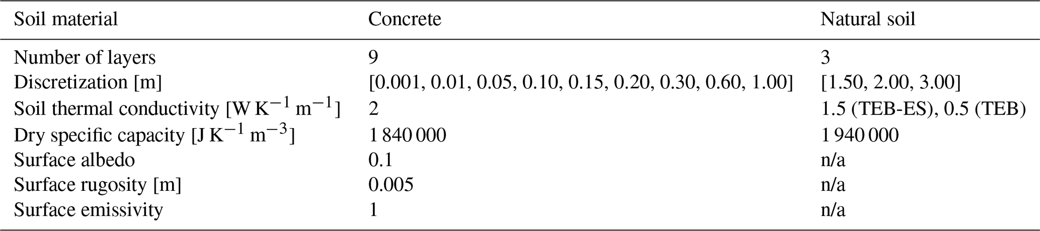
The road component of the TEB initial version described previously and represented in Fig. 1 is then modified to improve the representation of winter processes. The following sections describe the modification within TEB represented in Fig. 2 with a new ice content W_i and an improved representation of the snow mantle with the Explicit Snow (ES) model.

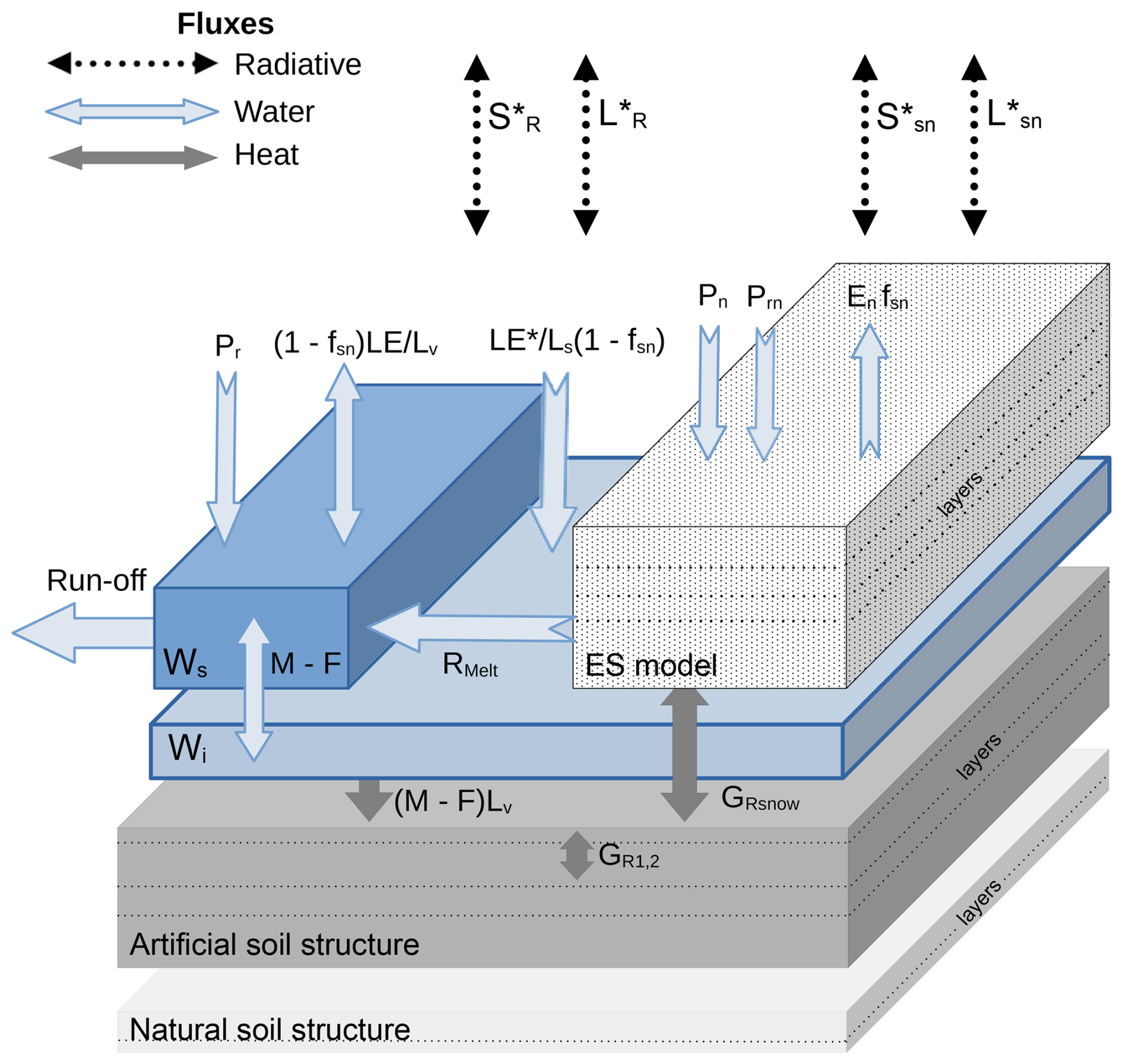
Figure 2 Schematic implementation of the new TEB model (TEB-ES) with the ice content W_i in light blue, the ES model in white, their interaction with the road surface in grey, and the water content W_s in blue. Heat, water, and radiation effects are represented by arrows with radiative fluxes $S_{\text{sn}}^{*}$ and $L_{\text{sn}}^{*}$ (net shortwave and net longwave over snow, respectively).

2.2 Implementation of road ice

To account for icy road conditions, we introduce a prognostic evolution of the amount of ice on the road. It is described by the state variable W_i (kg m⁻²), which represents the liquid water equivalent ice content. W_i evolves by phase-induced changes. First, it interacts with the water content W_s by melting and freezing. Second, it interacts with the atmosphere by deposition as shown in Fig. 2.

To be in agreement with the TEB modelling choices, the ice layer W_i energy, like the water reservoir W_s energy, is not explicitly modelled. Their temperatures are considered indistinguishable from the road surface. Thus, the processes involved in the ice evolution, freezing, melting, and sublimation directly impact the road surface temperature as follows:

$$\begin{array}{}\text{(4)}& {\displaystyle }{\displaystyle \frac{\partial T_{\text{road}}}{\partial t}}={\displaystyle \frac{\mathrm{1}}{d_{\mathrm{R}\mathrm{1}}}}\left(\right(\mathrm{1}-f_{\text{sn}}){\text{LE}}^{*}-(F-M\left)L_{\mathrm{v}}\right),\end{array}$$

with F representing the freezing rate ($\mathrm{kg}{\mathrm{m}}^{-\mathrm{2}}{\mathrm{s}}^{-\mathrm{1}}$), M the melting rate ($\mathrm{kg}{\mathrm{m}}^{-\mathrm{2}}{\mathrm{s}}^{-\mathrm{1}}$), f_sn the snow fraction on road, L_s the sublimation heat constant, and LE^* the solid–gas latent heat flux (W m⁻²). The ice content W_i changes according to

$$\begin{array}{}\text{(5)}& {\displaystyle }{\displaystyle \frac{\partial W_{\mathrm{i}}}{\partial t}}=F-M-(\mathrm{1}-f_{\text{sn}}){\displaystyle \frac{{\text{LE}}^{*}}{L_{\mathrm{s}}}},W_{\mathrm{i}}\ge \mathrm{0}.\end{array}$$

Freezing of water is an exothermic reaction while melting is endothermic. This will affect the energy balance at the surface of the road as shown in Fig. 2. Ice on the roads also changes the exchange coefficient, based on the aerodynamic resistance, resulting in modified turbulent exchange between the road and the first air layer in the canyon. For this process, we assume that the ice is at the first road layer temperature and the aerodynamic resistance is the same as that for water.

Several hypotheses arise from this parameterization. The fraction occupied by ice on the TEB road surface is set to 1. Thus, the ice layer can be partially or completely snow-covered depending on the snow fraction value f_sn. In addition, the ice content can grow without limitation as long as it is supplied by the freezing rate F of the available water content W_s, or by the ice deposition by sublimation on the snow-free fraction $(\mathrm{1}-f_{\text{sn}}){\text{LE}}^{*}/L_{\mathrm{s}}$. As the ice-layer energy is considered indistinguishable from the road surface, the snow-covered ice layer is transparent to the snow–road heat conduction flux G_Rsnow as shown in Fig. 2. Therefore, the ice-layer part that is snow-covered is insulated from the atmosphere and interacts only with the road surface by the melting process M.

The freezing rate, the melting rate, and the solid–gas latent heat flux equations for the ice evolution on the natural surface layer from Boone et al. (2000) are adapted to impermeable artificial surfaces. The insulating effects of the vegetation are removed as well as the phase change coefficients for subgrid-scale effects. The adapted water mass rates for impermeable artificial surfaces are therefore defined as

$$\begin{array}{}\text{(6)}& {\displaystyle }F& {\displaystyle }={\displaystyle \frac{\mathrm{1}}{\mathit{\tau }}}min\left(W_{\mathrm{s}},{\displaystyle \frac{max(O,T_{\mathrm{f}}-T_{\text{road}})}{C_{\mathrm{l}}{L}_{\mathrm{f}}}}\right),\text{(7)}& {\displaystyle }M& {\displaystyle }={\displaystyle \frac{\mathrm{1}}{\mathit{\tau }}}min\left(W_{\mathrm{i}},{\displaystyle \frac{max\left(O,T_{\text{road}}-T_{\mathrm{f}}\right)}{C_{\mathrm{l}}{L}_{\mathrm{f}}}}\right),\text{(8)}& {\displaystyle }{\text{LE}}^{*}& {\displaystyle }={\mathit{\rho }}_{\mathrm{a}}{\displaystyle \frac{\mathrm{1}}{R_{\mathrm{a}}{L}_{\mathrm{s}}}}\left[Q_{\text{sati}}\right(T)-Q_{\mathrm{a}}],{\text{LE}}^{*}\le \mathrm{0},\end{array}$$

with T_f the freezing temperature, L_f the latent heat of fusion of water, R_a the air aerodynamic resistance, ρ_a the air density, τ the characteristic timescale for phase change, and C_l the ice heat capacity thermal inertia coefficient described in Boone et al. (2000). The parameter τ is set to 25 000 s rather than the 3300 s used for natural soil in order to get realistic simulations for this study's experiments. Ice sublimation is assumed to be negligible because its evolution is small compared with F or M. Thus, when the road surface reaches the saturation specific humidity with Q_sati(T)≥Q_a, LE^* is set to 0. So ${\text{LE}}^{*}\le \mathrm{0}$, and deposition as frost on the road can occur. The melting and freezing process couples the evolution of the ice and water contents. Thus, the water reservoir evolution equation becomes

$$\begin{array}{}\text{(9)}& {\displaystyle }{\displaystyle \frac{\partial W_{\mathrm{s}}}{\partial t}}=R+R_{\text{melt}}-(\mathrm{1}-f_{\text{sn}})\text{LE}/L_{\mathrm{v}}-F+M,\end{array}$$

with F, M the freezing and melting rates for ice.

2.3 Improvement of the road snow processes with a multi-layer scheme

The thermal and liquid profiles of the snow mantle cannot be represented by averaged single-layer variables as in one-layer snow model schemes; they require multi-layer models instead (Etchevers et al., 2004). Cristea et al. (2022) showed that using several layers in snow models improves the realism of the heat changes and liquid transfers between the snow layers. Decharme et al. (2016) have also shown that converting a snow model from 3 to 5 layers leads to a more accurate soil temperature evolution. Explicit Snow (ES) (Decharme et al., 2016) is a multi-layer snow model that explicitly resolves the heat-energy balance. The prognostic variables are snow density, heat content, thickness for each snow layer, and albedo. Sun et al. (1999) suggested that at least three snow layers are needed to represent a snow thermal profile.

In this work, ES simulates the snow mantle evolution on a road modelled inside the local canyon geometry of TEB. The snow model is forced by the TEB variables. ES receives the computed shortwave radiation from the road sky-view factor and the trapped longwave radiation. It is also forced by the local atmospheric variables computed inside the canyon, such as the specific humidity and air temperature. Finally, ES intercepts the snow precipitation and the liquid precipitation. Unlike the one-layer snow scheme (1-L), ES computes the impact of the liquid precipitation on the snow mantle. The total liquid precipitation rate R ($\mathrm{kg}{\mathrm{m}}^{-\mathrm{2}}{\mathrm{s}}^{-\mathrm{1}}$) is split into a fraction that enters the snowpack with P_rn ($\mathrm{kg}{\mathrm{m}}^{-\mathrm{2}}{\mathrm{s}}^{-\mathrm{1}}$) and a fraction that is intercepted by the water reservoir with P_r ($\mathrm{kg}{\mathrm{m}}^{-\mathrm{2}}{\mathrm{s}}^{-\mathrm{1}}$):

$$\begin{array}{}\text{(10)}& {\displaystyle }& {\displaystyle }{P}_{\mathrm{rn}}=f_{\text{sn}}R,\text{(11)}& {\displaystyle }& {\displaystyle }{P}_{\mathrm{r}}=R(\mathrm{1}-f_{\text{sn}}).\end{array}$$

The snow fraction, f_sn, defined by Eq. (1) with respect to the TEB initial version is modified as follows:

$$\begin{array}{}\text{(12)}& {\displaystyle }{\displaystyle }{f}_{\text{sn}}=min(\mathrm{1},D_{\mathrm{s}}/\mathrm{0.01}).\end{array}$$

So f_sn=1 when the total snow mantle depth D_s is greater than 0.01 m.

The atmospheric variables in the TEB canyon are modified by this new snow scheme. For both the 1-L and ES options, the amount of radiation received by the snow-free fraction of the road is weighted by the snow cover. The snow–atmosphere interaction is modified by the ES scheme. The net heat flux and the sensible, latent, and radiative fluxes all depend on the local variables inside the snow mantle simulated by ES.

At the bottom of the snow mantle, ES is coupled with the impermeable road surface. Liquid water leaving ES is treated as in 1-L: it is transferred to the water reservoir and then taken into account in the road surface energy balance or it leaves the system as runoff if W_s reaches W_smax. However, the heat conduction between the road surface and the lower snow layer (G_Rsnow) is not treated as in 1-L: the ES scheme is implicitly coupled to the road surface following the procedure of Masson and Seity (2009), to improve stability. Heat conduction between 1-L and the road component heat equations is strictly explicit. It impacts the road surface energy balance as in Eq. (2).

The mass conservation equation for the total snowpack in TEB-ES is

$$\begin{array}{}\text{(13)}& {\displaystyle }{\displaystyle \frac{\partial W_{\text{snow}}}{\partial t}}=P_{\mathrm{n}}+P_{\mathrm{rn}}-R_{\text{melt}}-E_{\mathrm{n}}.\end{array}$$

W_snow is the product of the average snowpack density and the total thickness. It corresponds to the total snow water equivalent (SWE) (kg m⁻²). P_rn is the liquid precipitation rate defined in Eq. 10, P_n the snowfall rate, R_melt ($\mathrm{kg}{\mathrm{m}}^{-\mathrm{2}}{\mathrm{s}}^{-\mathrm{1}}$) the melt rate, and E_n ($\mathrm{kg}{\mathrm{m}}^{-\mathrm{2}}{\mathrm{s}}^{-\mathrm{1}}$) the total latent heat flux caused by evaporation and condensation.

Unlike in 1-L, each ES layer is characterized by a liquid water content of the snow W_li. Index i refers to the layer. It is modelled as a series of bucket-type reservoirs and the layer liquid water content W_li stays <10 % of the layer snow mantle mass represented by W_limax, with

$$\begin{array}{}\text{(14)}& {\displaystyle }{\displaystyle \frac{\partial W_{\mathrm{l}i}}{\partial t}}=R_{\mathrm{l}i-\mathrm{1}}-R_{\mathrm{l}i}+{\displaystyle \frac{F_{\mathrm{s}i}}{L_{\mathrm{f}}}},\end{array}$$

with the condition $W_{\mathrm{l}i}<W_{\text{l}imax}$ and

$$\begin{array}{}\text{(15)}& {\displaystyle }{\displaystyle }{R}_{\mathrm{l}\mathrm{0}}=P_{\mathrm{rn}}-(\mathrm{1}-{\mathit{\chi }}_{\mathrm{1}})E_{\mathrm{n}},\end{array}$$

where R_li−1 and R_li are the water flows between the layers i−1 and i ($\mathrm{kg}{\mathrm{m}}^{-\mathrm{2}}{\mathrm{s}}^{-\mathrm{1}}$), F_si is the phase change heat flux (W m⁻²) that represents the sum of two terms, the available energy for snow to melt and the available energy for the liquid water to freeze (considered as snow W_snow), R_l0 is the flux at the snow surface, and χ₁ is the fraction of the total mass of the frozen surface layer, defined as

$$\begin{array}{}\text{(16)}& {\displaystyle }{\displaystyle }{\mathit{\chi }}_{\mathrm{1}}=\mathrm{1}-{\displaystyle \frac{W_{\mathrm{l}\mathrm{1}}}{W_{\text{snow1}}}}.\end{array}$$

The snow layer density prognostic variable ρ_si (kg m⁻³) changes because of a few factors, such as the weight of the overlying snow, the settling mainly due to fresh snowfall, the thermal metamorphism, and the viscosity of the snow. Also, the fresh snowfall usually reduces the uppermost layer density and is defined as

$$\begin{array}{}\text{(17)}& {\displaystyle }{\displaystyle }{\mathit{\rho }}_{\text{new}}=a_{\text{sn}}+b_{\text{sn}}(T_{\mathrm{a}}-T_{\mathrm{f}})+c_{\text{sn}}(V_{\mathrm{a}}{)}^{\mathrm{1}/\mathrm{2}},\end{array}$$

where T_a is the air temperature inside the canyon in Kelvin, V_a the wind speed, and coefficients a_sn=109 kg m⁻³, b_sn=6 $\mathrm{kg}{\mathrm{m}}^{-\mathrm{3}}{\mathrm{K}}^{-\mathrm{1}}$, and c_sn=26 kg. Melting, infiltration of rainwater, and retention of snow melt also affect the snow layer density as described in Boone and Etchevers (2001).

The snow mantle is slightly transparent to the solar radiation flux. The snow mantle heat-balance equation is modified at each layer by this positive heat flux. The solar transmission heat flux is a negative exponential of the snow depth and the extinction coefficient for shortwave radiation products. This flux is weighted by the snow surface albedo.

In ES, the snow surface albedo process is adjusted for natural environments and computed as in Decharme et al. (2016). The impact of human activity, such as pollution sources, on the whiteness of snow is not considered. Thus, the albedo equation and parameters used in 1-L from Lemonsu et al. (2010) are used in replacement. This directly impacts the solar radiation transmission heat flux.

3 Experimental set-up and assessment

3.1 Model configuration

This study compares the TEB initial version released in SURFEX v9.0 with the modified version called TEB-ES, with the road component processes shown in Figs. 1 and 2, respectively. The TEB-ES version used in this study is published in the repository Colas (2024), focusing on the processes related to snow and ice described previously. Both models are configured in a similar way in order to evaluate the impact of the new processes at the locations selected for this study: Col de Porte in France and Hajala in Finland. Two benchmark road weather models are established and compared with TEB and TEB-ES performance. First, the heat-balance model ISBA-Route/CROCUS described in Bouilloud and Martin (2006), in operation at the French national meteorological office, is used in comparison at the Col de Porte location. ISBA-Route/CROCUS has previously been shown to perform well at this site (Bouilloud and Martin, 2006). Therefore, it is used in comparison at this location only. CROCUS is a more complex snow model than ES and is coupled to the surface of ISBA-Route. CROCUS and ES share many similarities, but CROCUS can explicitly calculate snow metamorphism, including grain size and shape evolution, which impact the mechanical properties and albedo of the snow mantle (Vionnet et al., 2012). Secondly, at each experimental location, a simple statistical model described in Kršmanc et al. (2013), which is built with a multiple linear regression (MLR) method, is used to predict road surface temperature. Simple empirical models are valuable for assessing the need to construct complex physical models for predicting surface variables (Lipson et al., 2024). The best predictive variables for the MLR are found using a stepwise regression procedure as explained in Appendix A, using the same available forcing variables that are used as input for the heat-balance model.

TEB is designed for urban areas, but it needs to be adapted for validation sites located in open areas where the pavement is constructed without adjacent structures. The local canyon geometry configuration of the model cannot be completely removed. So, we flatten the canyon geometry to the limit. The canyon aspect ratio was set to 0.0001, which causes the sky-view factor of the road to be close to 1. This nullifies the radiative trapping of the canyon. The building fraction is set to 0.0001 to limit interactions between the air inside the canyon and the TEB building component. With these settings, TEB is considered to simulate a road in open surroundings. The surface boundary layer option is activated and computes explicit atmospheric variables inside the urban canyon (Masson and Seity, 2009). The explicit calculation of the longwave exchanges is also activated. We set the physical parameters of the pavement structure described in Table 1 to be in agreement with Bouilloud and Martin (2006) for a French highway. The natural soil under the artificial structure is initialized in TEB by the thermal conductivity of the dry soil, whereas for TEB-ES it is initialized with the thermal conductivity of the moist soil (Bouilloud and Martin, 2006). Indeed, at our experiment site, water infiltrates beneath the road from surrounding natural soil. For the Finnish experiment in this article, the TEB-Hydro component is enabled in order to simulate the water drainage on the roads (Bernard et al., 2020), and W_smax is set to 0.6 kg m⁻² rather than 1 kg m⁻² because of the different road properties.

A straightforward parameterization of snow removal operations is implemented in TEB, TEB-ES, and ISBA-Route/CROCUS. Within these models, snow depth and ice content are set to zero when an operator clears the snow. This parameterization is adapted for the snow removal procedures carried out at the experimental sites presented in the next section. In the Col de Porte experiment, snow and ice are reset to 0 on the known date of snow removal by a manual operator. In the Hajala experiment, the exact dates of winter maintenance activities are unknown. So, snow and ice are reset to 0 at 06:00 UTC in the models.

3.2 Experiments

The models are mainly forced by the on-site observations at the experimental set-up location. They are first assessed at the Col de Porte measurement site of Météo-France. It is located at an altitude of 1325 m in the Chartreuse mountain range in the Alps (45.30° N, 5.77° E). This site is in a grassy meadow surrounded by a coniferous forest; it is covered by snow several months a year. In operation since 1959, the Col de Porte Météo-France site is equipped with standard meteorological and snow mantle sensors (Morin et al., 2012). It is a European reference for the study of snow-covered surfaces, thanks to the meteorological conditions and its collection of sensors. Thus, data from this site have been exploited to validate many snow models Decharme et al., 2016; Vionnet et al., 2012; Cristea et al., 2022 and even used for large snow model intercomparison projects (Etchevers et al., 2004). During three winters (1997/98–1999/2000), the Col de Porte hosted a large experiment to study the snow–road interface within the GELCRO project (Muzet et al., 2000). An artificial pavement (2 m×3 m) equivalent to a French highway, shown in Fig. 3, was installed at the site (Bouilloud and Martin, 2006). The road surface temperature, with a probe inside the artificial structure, and the snow depth were monitored. The snow cover was frequently cleared by an operator throughout the entire experiment. The dates of these removal operations are known. This experiment was used to evaluate the ISBA-Route/CROCUS model (Bouilloud and Martin, 2006) used for road maintenance purposes, which is our heat-balance road weather benchmark model for this study.

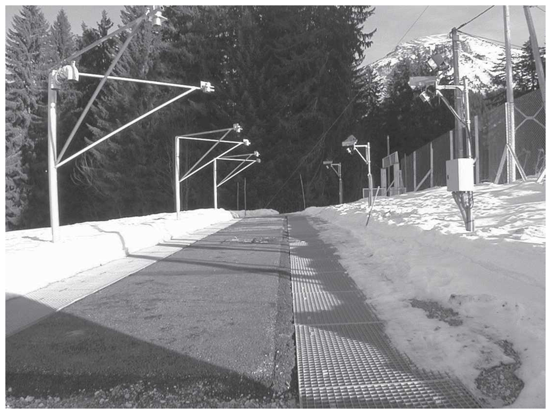
Figure 3 Col de Porte experimental artificial soil during the GELCRO campaign, extracted from Bouilloud and Martin (2006).

TEB-ES is assessed and compared with TEB, ISBA-Route/CROCUS, and MLR. The heat-balance models are forced hourly by the local atmospheric measurements at the nearby meteorological station. The 6 min precipitation measurements are aggregated every full hour to give a precipitation intensity (mm h⁻¹). The precipitation phase is selected by assuming that it is rainfall when the air temperature is >1 °C and snowfall when the air temperature is ≤1 °C as done in Bouilloud and Martin (2006). Jennings et al. (2018) confirmed that the air temperature of 1 °C is the average temperature of separation of the precipitation phase in the Alps. But this assumption can often fail (Jennings et al., 2018). For the other atmospheric measurements, the value closest to the whole hour is considered. The hourly surface observations provide validation data for the models. The models are evaluated with the surface observations of the artificial pavement.

Next, a site with recurring snowy and ice road conditions outside of controlled experimental conditions was selected to assess TEB, TEB-ES, and MLR. In southern Finland, these kinds of conditions are normal in winter and the temperature crosses zero degrees multiple times during the winter season, making surface condition forecasting a challenge. Fintraffic has installed numerous road weather stations to monitor atmospheric variables (wind speed, air temperature, humidity, and precipitation), road surface temperature, and road conditions. The road surface temperature sensors are manufactured by Vaisala and measure road surface temperature with asphalt embedded sensors. Many stations also have optical instruments that measure the thickness of the water, ice, and snow layer. Among several stations with the most sensors, the Salo Hajala road weather station (60.435° N, 22.969° E) shown in Fig. 4 has been arbitrarily selected. From now on it is called just “Hajala”, for the sake of simplicity.

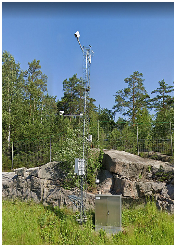
Figure 4 Salo Hajala road weather station in Finland, © Google Street View 2024.

To validate the model, we used the road surface temperature observations from the dataset of Karsisto (2018) used in the study conducted by Karsisto and Lovén (2019). Corresponding atmospheric observations measured by the Salo Hajala road weather station have been provided by the Finnish Meteorological Institute and are available in the Zenodo of Colas (2024). Observed wind speed, air temperature, humidity, and precipitation from the Hajala road weather station are used as atmospheric forcing in the model and processed in the same way as the Col de Porte forcing. Since there is no radiation measurement at the Hajala road weather stations, shortwave and longwave radiation were extracted from ERA5 reanalysis at the closest grid point (Hersbach et al., 2020). Surface measurements including road surface temperature, water/ice contents, and snow water equivalent (SWE) are then used to validate the models. The studied period was from October 2017 to May 2018.

In many cases, optical instruments are considered unreliable for detecting, with precision, road conditions subject to anthropic effects and winter maintenance road operations. Indeed, optical sensors always failed to distinguish between ice and snow content on the road surface. In the Hajala experiment, on the 706 snow occurrences and 743 ice occurrences measured, the sensors recorded 706 occurrences of both ice and snow at the same time, and the other 37 hourly occurrences for ice are at the beginning or at the end of a snow event. Anthropic effects such as traffic and winter maintenance directly influence the physical variables. In addition, an optical sensor might only see the top of the snow or ice layer and is unable to measure the actual thickness. For these reasons, the ice and snow mass contents measured by the optical sensor should not be used to validate the models quantitatively but qualitatively as occurrences. They are compared, in the Hajala experiment, with the snow and ice output variables from the models transformed as occurrences.

Statistical scores are calculated hourly at the Hajala site for the whole simulation, similarly to the Col de Porte experiment. The scores in Tables 3, 4, and 6–8 are calculated from the confusion matrices that report the numbers of true positives (TP), false negatives (FN), false positives (FP), and true negatives (TN). They are calculated as follows: detection rate $=\text{TP}/(\text{TP}+\text{FN})$, missed event rate $=\text{FN}/(\text{TP}+\text{FN})$, false positive rate $=\text{FP}/(\text{FP}+\text{TN})$, and false discovery rate $=\text{FP}/(\text{TP}+\text{FP})$. These metrics help to evaluate the models' performances for important thresholds, in particular for decision-making in the context of road weather forecasts.

Table 2 Scores for TEB, TEB-ES, and the benchmarks (ISBA-Route/CROCUS, MLR) at the Col de Porte location during winter 1998–1999.

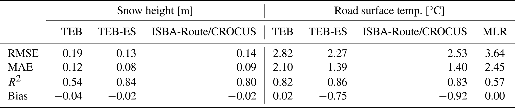
Table 3 Performance of TEB, TEB-ES, and the benchmarks (ISBA-Route/CROCUS, MLR): surface temperature occurrence, below 0.5 °C, at 1 h time steps, at the Col de Porte location during winter 1998–1999.

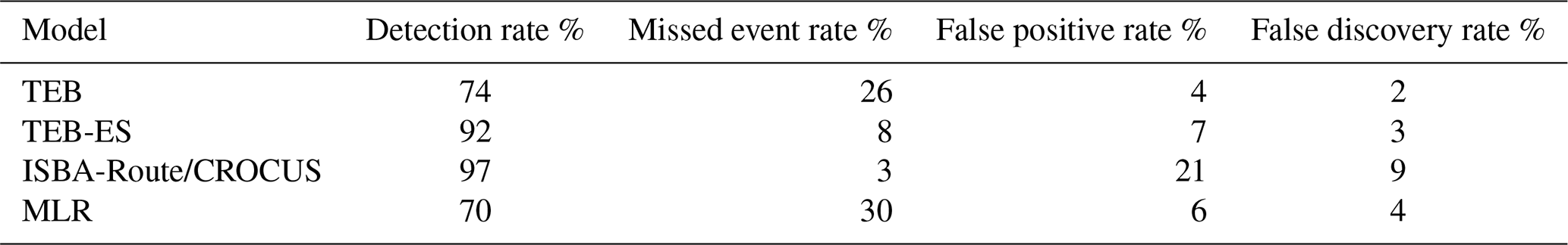
Table 4 Performance of TEB, TEB-ES, and ISBA-Route/CROCUS: snow depth occurrence greater than 0.5 cm, at 1 h time steps, at the Col de Porte location during winter 1998–1999.

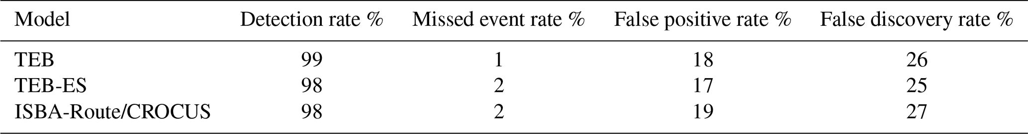
Table 5 Road surface temperature scores for the Hajala site during winter 2017–2018.

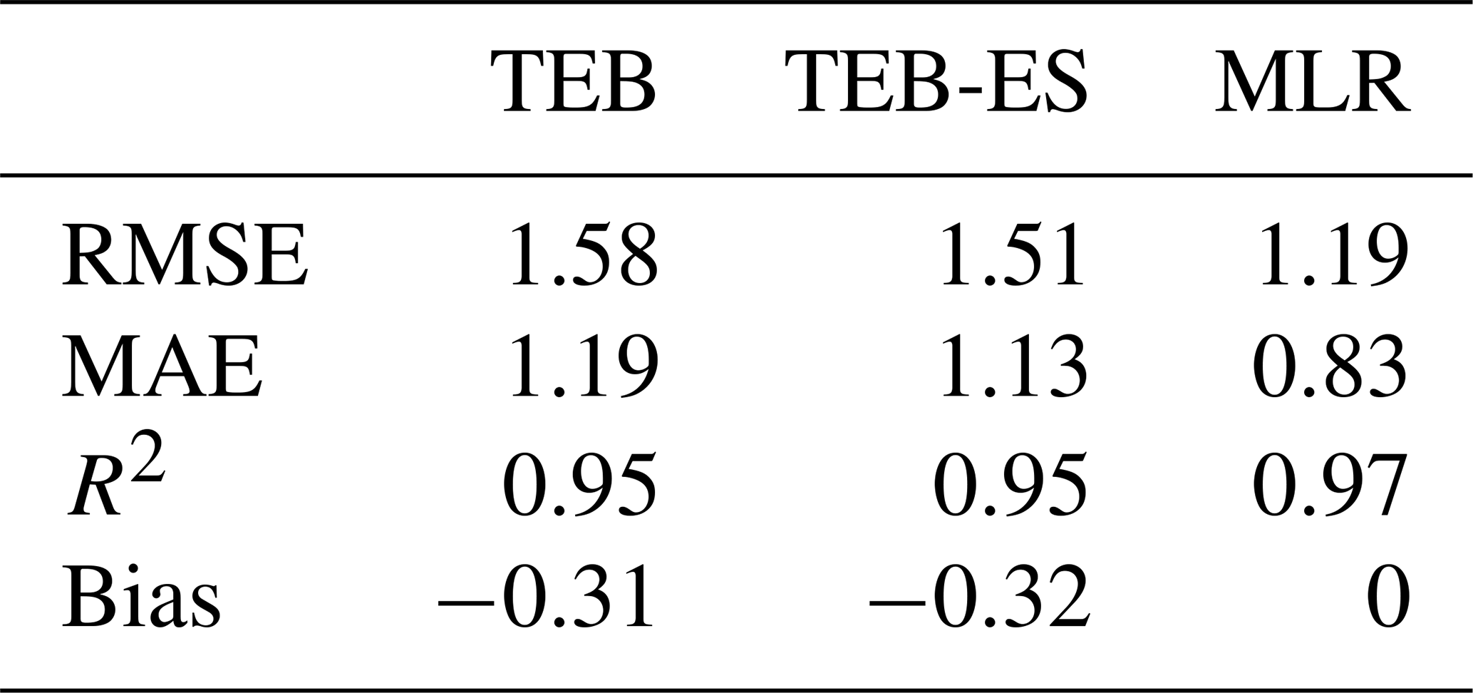
Table 6 Performance of TEB, TEB-ES, and MLR: surface temperature occurrence below 0.5 °C, for 1 h time steps, at the Hajala site during winter 2017–2018.

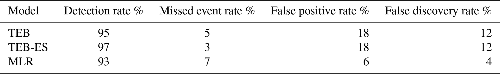
Table 7 Performance of TEB and TEB-ES: SWE occurrence greater than 0.01 mm, for 1 h time steps, at the Hajala site during winter 2017–2018.

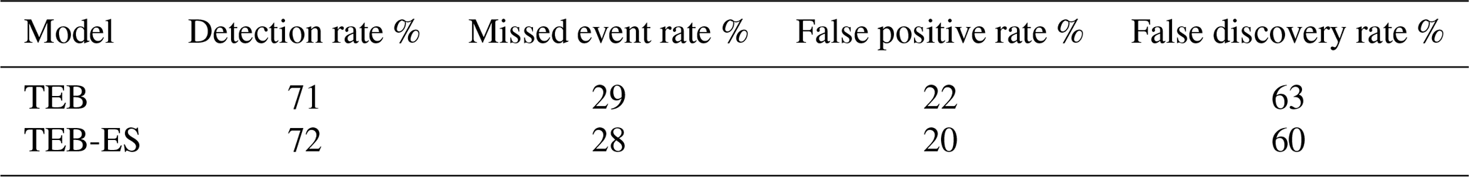
Table 8 Performance of TEB and TEB-ES: ice depth occurrence greater than 0.001 mm, for 1 h time steps, at the Hajala site during winter 2017–2018.

4 Evaluation at the Col de Porte site

First, we compare the performance of TEB, TEB-ES, and the benchmarks at the Col de Porte meteorological site during the GELCRO campaign. They are forced by the in situ measurements and set up to compute the physical variables from 21 October 1998 06:00 UTC to 14 May 1999 04:00 UTC in a continuous simulation over the whole time span. In this reference experiment, the implemented new winter processes are evaluated to see whether they have a positive impact on the model performance and the physics consistency. Snow depth and road surface temperature simulations are compared with the observations.

4.1 7–18 November period

The time range extracted from the simulation from 7 to 18 November in Fig. 5 shows typical snow conditions at the measurement site with five snow events. During this period, the road was cleared three times by hand. Thus, in the models, on 13 November at 12:00 UTC, on 16 November at 11:00 UTC, and on 17 November at 17:00 UTC, the snow heights and the ice contents are reset to 0.

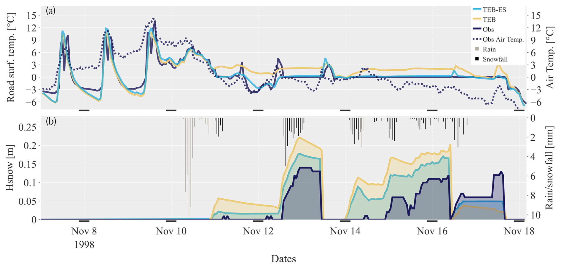
Figure 5 Comparison between the models and the observations at the Col de Porte location. (a) Road surface temperature (modelled and observed) and observed air temperature, (b) snow height (modelled and observed) and observed rain/snowfall with a reversed y axis.

On 7–9 November, a synoptic high pressure centred over western Europe brought calm weather. Conditions were dry with positive air temperature and clear skies. The observed daily evolution of the road surface temperature is accurately simulated by TEB and TEB-ES. Both simulations are nearly identical, except that TEB-ES has a reduced cold bias during the evening and night. Here, the road surface temperature is driven by road–atmosphere interaction and the pavement conduction. The soil–atmosphere interaction in the absence of ice or snow has not been changed in the new version of TEB. But the moisture conductivity in the natural soil under the pavement added in TEB-ES, as seen in Table 1, leads to improved pavement heat restitution and reduces the cold bias by 0.5 °C.

Several weather perturbations occurred during the following days. The first low-pressure system reached the station on 10 November. Rain fell in the afternoon, followed by snow in the evening. TEB-ES simulates smaller snow depths than TEB (around 2.7 cm smaller for the episode). ES melts almost all snowpack and is closer to the observations, as shown in Fig. 5. Therefore, the TEB-ES road temperature follows the observations that report a negative air temperature, whereas the TEB road surface temperature is insulated from the atmosphere by the snow mantle; its road surface heat change is driven by pavement conduction and snow–road heat transfer. TEB-ES road surface simulation is better than TEB on 11 and 12 November. After a small observed snowfall in the afternoon of 12 November, the snow depth evolution is well computed by TEB-ES, with less than a 2 cm difference with the observations. TEB adds fresh snow to the previous snow mantle on the road and leads to a snow cover 6 cm higher than the measured value.

From 14 to 17 November, a low-pressure system persisted over eastern Europe with several rainfall and snowfall events before a strong ridge brought back high pressure and clear skies. At the beginning of this event, the precipitation forcing is wrong; it was rain rather than snowfall that affected the location. This explains the excessive snow cover in both models. The following snow event is well modelled by both models. ES simulates the fresh snow accumulation more accurately due to the mixed composition density of fresh and old snow layers (Decharme et al., 2016). In addition, the road surface temperature is better modelled by ES with a mean absolute error (MAE) of 0.3 °C. 1-L has a MAE of 1.4 °C during this event. This was a typical isothermal event with a snow–pavement interface layer at constant freezing temperature. This effect is poorly represented by the 1-L snow model.

4.2 Statistical results

Twenty-three snow events occurred during the date range from 21 October 1998 at 06:00 UTC to 14 May 1999 at 04:00 UTC at the Col de Porte, which is a large enough sample to show statistical differences between the models. The scores displayed in Table 2 show notable differences in the performance of the road surface temperature and snow height simulations. The heat-balance models outperform the statistical benchmark. In Table 2, the absence of bias in the TEB road surface temperatures is explained by several seasonal biased scores that compensate. Indeed, Fig. 6 shows significant seasonal temperature differences from the observations in TEB. For TEB-ES and ISBA-Route/CROCUS simulations, the seasonal temperature differences from the observations are much lower. TEB-ES's and ISBA-Route's road surface temperatures are more consistent with the observations than the TEB simulation, as shown in Table 2 and Fig. 6. Snow height is better simulated by TEB-ES than TEB in terms of RMSE, MAE, and R², as shown in Table 2. Multi-layer snow model coupling greatly improves the snow height and the road surface temperature performance.

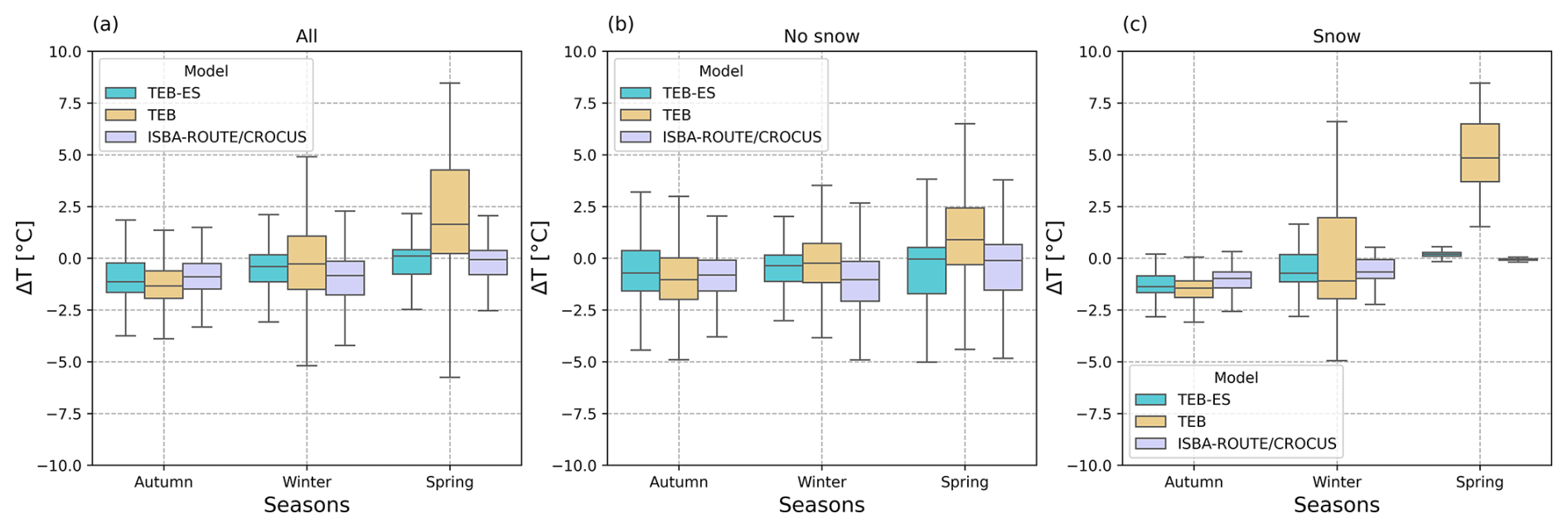
Figure 6 Seasonal road surface temperature difference comparison with the observations between TEB, TEB-ES, and the benchmark ISBA-Route/CROCUS. Figures with road condition partitioned for the situations: (a) all cases, (b) no snow observed, (c) non-zero snow observed. The boxes extend from the first quartile (Q₁) to the third quartile (Q₃), with whiskers up to the farthest point lying within 1.5× the interquartile range (Q₃−Q₁).

In addition, we evaluate the ability of the models to capture the occurrence of significant events that could compromise road safety. Tables 3 and 4 evaluate the ability of the models to predict potential dangerous conditions and snowy road condition occurrences, respectively. Similar confusion matrices are found for the models for snow height >0.5 cm, as shown by the similar rates in Table 4.

Larger differences are observed in road surface temperature simulations between heat-balance models in snow-covered isothermal situations. This is particularly visible during spring 1999, as shown in Fig. 6c, with snow-covered isothermal situations only. In these situations, the TEB road surface temperature is strongly biased, while TEB-ES and ISBA-Route/CROCUS show good performance. ISBA-Route/CROCUS has a slightly better performance than TEB-ES in these situations, due to the complexity of the CROCUS snow model. However, during one particular event in early spring, road surface temperature was very poorly simulated by ISBA-Route/CROCUS. These outliers are not shown in Fig. 6. The TEB-ES detection rate is much higher than TEB for road surface temperature <0.5 °C, as shown in Table 3, which can be attributed to snow-covered isothermal situations.

5 Evaluation at the Hajala site

In this section, we take advantage of the detailed observations at the Finnish Salo Hajala road weather station to further validate the physics of the model, in particular, in terms of water content, ice, and snow water equivalent (SWE) occurrences at the road surface. The model is set up to calculate the evolution of the TEB variables for about 6 months in a continuous run, from 23 October 2017 at 15:00 UTC to 1 May 2018 at 19:00 UTC.

5.1 17–26 January 2018 period

From 17 January 2018 to 23 January 2018, the Salo Hajala site was affected by a cold air mass with road temperatures below −3 °C (Fig. 7). Three light synoptic scale snow events impacted traffic conditions by causing snow cover on the roads. Then, on 24 January, the weather regime changed with a low-pressure system, which brought snowfall, then warmer air with rain.

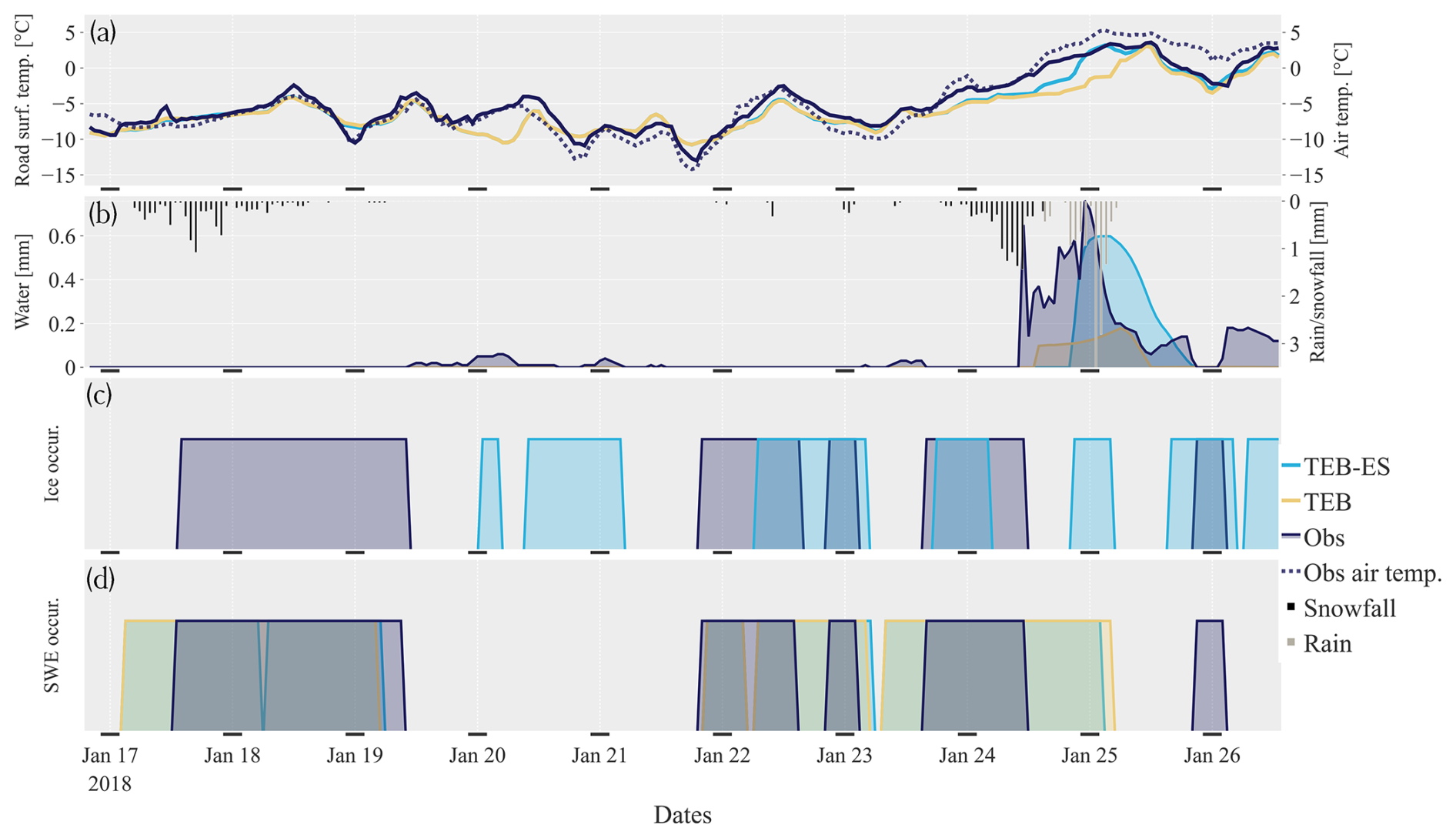
Figure 7 Comparison between TEB, TEB-ES, and the observations at the road surface on a road weather station at Hajala. (a) Road surface temperature (modelled and observed), (b) snow water equivalent (modelled and observed) and observed rain/snowfall, (c) ice on road (modelled and observed), (d) water on road (modelled and observed).

Small persistent snowfalls on 17 and 18 January in the morning are captured simultaneously as ice and snow measurements on the road until 19 January in the morning. This can be attributed to the solid content detection issue with the sensor, which usually does not discriminate between ice or snow. TEB and TEB-ES simulate the snow cover 8 h before the sensor measurement, as shown in Fig. 7. The models fail to match the time span of the event. This could be explained by the strong morning traffic commuting pattern that blew the snow away, removed the thin flake layer on the road, and then delayed the accumulation of the snow cover (Denby et al., 2013). However, the modelled road surface temperatures are consistent with the observed increasing trend during the afternoon of 18 January and show good performance.

On 19 and 20 January, during the nights, the sensor detected liquid water on the road surface. The sky was clear, and the rain gauge did not capture any rain. Thus, it may be spurious water detection by the sensor. TEB-ES simulates a possible small hoarfrost event that could have been classified as water.

Both models' snow mantle evolutions match the beginning of the observed SWE in late evening on 21 January. Afterward, the TEB and TEB-ES snow mantle evolutions are consistent with the observed snowfall. For this episode, the simulated snow occurrence is precise enough to return an accurate road surface temperature for both models.

In this 9 d period, the road surface temperature is well simulated for both models, with similar results. But TEB-ES significantly outperforms TEB on 24 January, which saw moderate snowfall followed by a rainfall episode. This shows an improved modelling of the snow mantle variables with ES for positive air temperatures. In both models, the simulated SWE occurrences are consistent with the observed snowfall but fail to match the observed SWE occurrences on the road. The snow removal parameterization at 06:00 UTC in the models appears to be an oversimplification of road maintenance operations such as salting or snow ploughing.

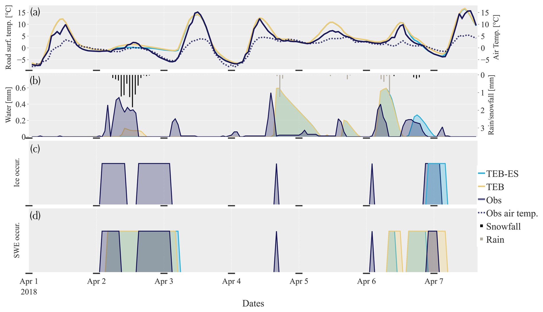
Figure 8 Comparison between TEB, TEB-ES, and the observations at the road surface on a road weather station at Hajala. (a) Road surface temperature (modelled and observed), (b) snow water equivalent (modelled and observed) and observed rain/snowfall, (c) ice on road (modelled and observed), (d) water on road (modelled and observed).

5.2 1–7 April period

Several cold conditions struck Hajala during this 6 d of this mid-spring period (Fig. 8). The road surface temperature is well simulated by both models, especially the diurnal cycle of surface temperature in clear sky conditions on 3, 4, and 7 April. For the road conditions, the models have varying degrees of success in representing the ice and SWE occurrences. In snow and ice-free conditions, the TEB and TEB-ES simulated water content evolutions are similar.

On 2 April at 02:00 UTC, uninterrupted moderate snowfall occurred at the station until 14:00 UTC under a low-pressure system. This standard snow event had probably been anticipated with brine injection during the night, since the water content observed increases as shown in Fig. 8. Since the salting effect is not modelled, both models poorly simulated the SWE occurrences captured by the Vaisala sensors. On 6 April, our precipitation type procedure misdiagnoses, twice, the precipitation types that fall into the rain gauge. This leads to two false positive light snow events on 6 April, at noon and in the afternoon, instead of wet road.

Clear sky conditions during the same night were cold enough to freeze the water on the road. Later, the road was salted, which melted the ice. In TEB-ES, the water produced by the snow mantle melting is frozen and the model accurately reproduces the observed occurrences on the road, which were presumably ice.

5.3 Statistical results

The overall TEB and TEB-ES road surface temperature performances shown in Table 5 are almost similar. TEB-ES is slightly better on RMSE and MAE but does not improve the R² and bias. For TEB-ES, the slight increase in performance is due to better simulation of the snow cover in snow-covered conditions, as shown in Fig. 9. On the panel (c), TEB-ES road surface temperature differences are less spread than TEB and are almost centred over 0 °C, revealing a seasonal performance trend in snow-covered situations with the heat-balance models. This is consistent with the behaviour of the Col de Porte experiment typical of snow isothermal events. However, the statistical benchmark significantly outperforms the heat-balance models with better RMSE, MAE, R², and bias. It is able to retrieve an accurate road surface temperature for each season, as shown Fig. 9. Even though the MLR predictions are mainly unbiased, Fig. 9 shows that in snow-covered conditions the road surface temperature simulated is slightly biased.

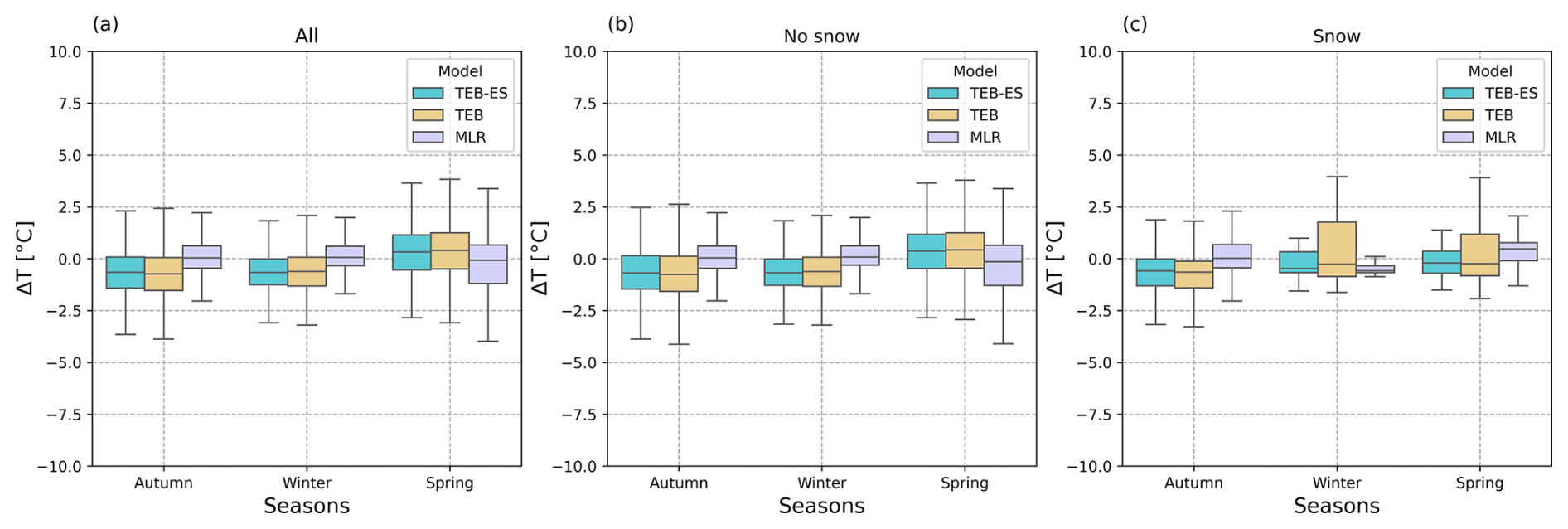
Figure 9 Seasonal road surface temperature difference comparison with the observations between TEB, TEB-ES, and MLR. Figures with road condition partitioned for the situations: (a) all cases, (b) no snow observed, (c) non-zero snow observed. The boxes extend from the first quartile (Q₁) to the third quartile (Q₃), with whiskers up to the farthest point lying within 1.5× the interquartile range (Q₃−Q₁) and without outliers.

As previously seen, the snow removal parameterization at 06:00 UTC in both TEB and TEB-ES is not complex enough to represent road maintenance operations such as salting or snow ploughing; this greatly influences the mass content evolution. For instance, freezing is simulated more often than observed, with 743 observed ice occurrences and 1368 modelled ice occurrences. As said in the sensor descriptions, the optical sensors are not able to distinguish between snow-covered or ice-covered road conditions on busy lanes. This explains the high missed event rate shown in Table 8. The scores are shown in Tables 7 and 8, but only a raw analysis can be extracted from these values. Therefore, the mass content performances cannot be compared between the models on this road, because of human activities.

However, the model simulations are consistent with physics, and tend to accurately represent the road conditions without human activities. The physical consistency of the models with the observed precipitation leads to high detection rates for SWE but a snow cover that is lower in observations than modelled (706 h observed, 1394 modelled by TEB, and 1417 modelled by TEB-ES), which leads to a >60 % false discovery rate on both models, as shown Table 7. In addition, the snow occurrence detection by the model shows <25 % false detection rate and >70 % detection rate. There are a high number of events without snow and ice.

6 Discussion

In this study, the performance evaluation of TEB and its modified version TEB-ES has been carried out in open surrounding areas to investigate whether this urban climate model can accurately reproduce artificial surface conditions predicted by road weather models in winter. We isolated the winter surface processes from other physical interactions by limiting the current experiments to open environments. The surroundings are limited to a few trees and no buildings. Although urban climate and road weather models mainly focus on simulating summer and winter conditions, respectively, we had attempted to bridge the gap between both model types by improving the TEB winter condition modelling by including new processes from road weather models.

TEB and TEB-ES simulations demonstrated physical consistency with the reality. The new developments in TEB-ES improve the performance of the road surface simulation in winter conditions, as seen on the 1998–1999 Col de Porte winter experiment, while beating the ISBA-Route/CROCUS road weather model in operation at Météo-France and even outperforming the in-sample statistical benchmark. TEB-ES appears well suited to simulate the surface response to atmospheric variables in artificial environments. The urban climate model is less effective for roads with human activities with snow ploughing, salting, and traffic, as shown in Hajala experiments. The prediction of the road surface temperature variable is better for TEB-ES than for TEB but they are both outperformed by the in-sample MLR benchmark.

Our study suggests that new developments within TEB are interesting for artificial surface predictions but are flawed for roads impacted by human activities. Indeed, overall model performance for the Finland experiment is poorer than for the Col de Porte experiment, as shown by the experiment's analysis and scores. This inferior performance is caused by several factors caused by human activities: errors in modelling snow removal, salting not modelled, or traffic effects not modelled (snow compaction and heating effects). In fact, traffic has a large effect on snow compaction: it reduces the snow depth and leads to measurement errors. In addition, Finland's winter road maintenance operator salts major roads whenever a slippery road condition is observed or forecast. Snow ploughing and salting is roughly simulated in the models by mechanical snow and ice removal every morning at 06:00 UTC in the Hajala experiment. The actual effects and timings of winter service vehicles are more complicated and impact the water contents and the surface heat energy. Salting indirectly affects road surface temperature by melting the snow cover that insulates the road from the atmosphere. Other measurement errors and sources of uncertainty may decrease the reliability of numerical experiments: lack of precipitation detection by the rain gauge, errors in distinguishing between snow and rain, sensor detection errors, and radiation forcing errors from the ERA5 reanalysis.

The Col de Porte simulations have better performance since no human activity impacts the different variables. This allows us to evaluate in detail the snow–road coupled behaviour in the models with the 1-L and ES snow models. The performance of the TEB-ES road surface temperature appears similar to the heat-balance road weather models at other locations (Meng, 2017; Nuijten, 2016; Denby et al., 2013). Some of these models have been tested in open environments, while others have been tested in urban areas. The main differences in snow height between the TEB and TEB-ES models can be summarized by three processes. First, the TEB-ES snow depth tends to be smaller than the TEB snow depth at the beginning of the events. Heat transfer between the pavement and the snow is better represented in TEB-ES. In addition, fresh snow properties and accumulation on old snow cover are also better modelled in TEB-ES because of the modelling of a specific density for each layer in the model. Secondly, the TEB-ES snow mantle tends to be higher than the TEB a few hours after each snowfall. The snow density of TEB follows a simple formulation with an exponential law to represent the ageing of the snow mantle, while the density of TEB-ES is affected by weight compaction, melting, rainwater infiltration, and snowmelt retention. Third, in snow-covered isothermal situations, there are large differences between TEB and TEB-ES. These isothermal situations are common during early winter and spring snowfalls, when the radiative forcing is high. The pavement returns the energy stored in its structure to the snow cover. The lower layers of the snowpack melt, causing liquid water to drain. In ES, as in the CROCUS snow model, the lower snowpack reaches its maximum liquid water content and the snowpack temperatures are at the freezing point. Thus, in TEB with the simple 1-L snow model, snow–soil heat transfer is underestimated. The difficulty of snow models with one or few layers in representing the evolution of the SWE in the spring melt season has also been shown by Cristea et al. (2022). Overall, the TEB-ES snow height follows the observed evolution more closely, as shown by the significantly higher R². There are some important differences between the snowpack evolution of TEB-ES and ISBA-Route/CROCUS but the overall snowpack heights and road surface temperature in observed snow-covered situations are close. In one snow-covered event in early spring (not shown here), ISBA-Route/CROCUS has a very large error in simulated surface temperature, unlike TEB and TEB-ES. This is caused by the different snow fraction formulation between TEB and ISBA-Route.

Comparison of heat-balance models with statistical benchmarks provides interesting insight for further studies. The artificial surface is a low-inertia and simple enough system with easily modelled behaviour, as shown by the good in-sample MLR performance in the Finland experiment. Although this behaviour is true in an open environment, more validation is needed with roadside components, trees, or buildings. The in-sample MLR Hajala simulation, which has been trained using observed road surface temperature is also capable of correcting the forcing errors and captures the impacts of human activities. So, these components could be systematic and cyclical enough to be easily modelled. It means that there is potential for further studies to take into account these effects in the heat-balance models. In both experiments, MLR models struggle to simulate the road surface temperatures when snow-covered. This leads to poor performance on Col de Porte with a mostly snow-covered road during the 6 month experiment. It suggests that the snow–road coupling is crucial for the heat-balance model performances. Indeed, it is difficult to capture surface physics when the road surface temperature is insulated from the atmosphere by the snow mantle. More complex statistical methods are needed, such as recurrent neural networks, to take into account the long-term system inertia and model the coevolution of road surface temperature with road mass contents. However, training such models is likely to require the acquisition of accurate mass content observations.

Further research is needed to address modelling and evaluation limitations from this study. First, ice content modelling could be improved by finding a better estimate of the characteristic timescale for phase change τ, set now at 25000 s. This parameter value should be evaluated more rigorously in more experiments to get a better estimate. Then continuous effects from traffic, such as heating, snow compaction, turbulence, and splash, and intermittent effects such as winter maintenance activities are not modelled in TEB and TEB-ES despite their major impact on artificial surface conditions (Fujimoto et al., 2014; Giudici et al., 2019). This should be addressed in future work to match the mass content observations on busy road lanes, as in the Hajala experiment. In most road weather models, some of these effects are taken into account, with different levels of complexity (Denby et al., 2013; Karsisto and Horttanainen, 2023), going from simple linear modelling to full parameterization of the salting effects. Finally, in this study, we assessed the model on open environments only, to analyse the specific process at the surface. So, further research is needed to evaluate these new processes in complex environments, such as facing walls or roadside trees (Lemonsu et al., 2012). TEB should behave well in such complex environments, as they have been the focus of TEB developments for the past decades. To complete the evaluation of the model, particularly for using TEB coupled to an atmospheric model, winter fluxes should be extensively assessed at many locations. This could be performed following the Urban-PLUMBER initiative, with extensive model comparisons (Lipson et al., 2024). In relation with the former comment, we propose, in Appendix B, a snow removal parameterization in urban environments to support further studies.

7 Conclusions

Bringing together the best of urban climate and road weather models would benefit both communities. In the urban climate community, cold conditions have been largely understudied, allowing many unknowns about the urban climate response to harsh winter conditions. This study is a first step toward addressing the literature limitations on this topic by improving the modelling of artificial surface winter conditions, which have a major impact on cold city climates. Of particular relevance to the road weather community, improved modelling of artificial surface conditions in an urban climate model could improve the accuracy of road condition predictions in complex environments.

A modified version of TEB from SURFEX-TEB v9.0 has been developed to improve modelling of winter processes. We incorporated basic ice content prognostic evolution to depict frost and water freezing on the surface and a new, precise, snow model that is coupled with the TEB road component. The new physics has been verified at two different winter sites. One experiment was carried out under controlled conditions at Col de Porte in the French Alps, while the other was based on a busy road with traffic and with recurrent winter maintenance operations in Hajala, Finland. TEB-ES significantly improved the surface condition prediction accuracy for the Col de Porte controlled experiment, outperforming the benchmarks provided by ISBA-Route/CROCUS and MLR. Periods that are conducive to slippery conditions are well detected in TEB-ES. During snowfall, the snow coverage of the artificial surface is accurately simulated. Road surface temperatures are also more accurately predicted for both the Hajala and Col de Porte experiment with TEB-ES. However, the Hajala road weather station experiment has shown that further developments are needed to account for anthropic effects. Future works on road heating by traffic, salting, water splashing, and snow compaction are expected to improve the model performance in terms of snow and ice content for high-traffic managed roads.

Appendix A: Statistical benchmark model

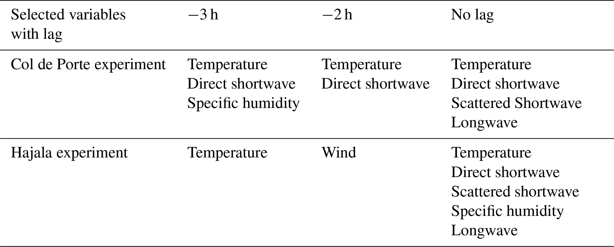
In this study, two multiple linear regressions (MLRs) are developed for predictive purposes as a benchmark for the Col de Porte and Hajala experiment. The models are developed using the same knowledge that the heat-balance models use to simulate the temperature of the road surface. Thus, the wind speed, wind direction, solar radiation – direct and scattered – longwave radiation, air temperature, specific humidity, and pressure forcings are used as input data for the MLR models. Following Kršmanc et al. (2013), the hourly forcing variables from lags of 3 and 2 h and from no lag are concatenated. In total, 24 explanatory variables are considered by the models. A backward feature selection procedure is performed to avoid overfitting. The selection is made using the adjusted-R² criterion, which, unlike the R², is not monotonically nondecreasing by the number of explanatory variables. The results of the selection procedure are drawn in Figs. A1 and A2 with cross-validation estimator performance uses. The maximum mean adjusted-R² calculated by the selection procedure in both experiments, shown in Figs. A1 and A2, is used to select the variables needed for the models. The maximum mean values of adjusted-R² are, respectively, 0.678 and 0.967 for the nine and seven extracted variables shown in Table A1. In this paper, the model predictions are made in-sample. This means that the data used for inference are also used to learn the model.

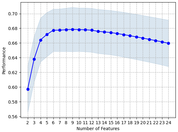
Figure A1 Sequential feature selection performance with 20 cross-validation steps, for the multiple linear regression at Col de Porte with the adjusted-R² as a function of the number of backward selected features, with 0.95 confidence interval.

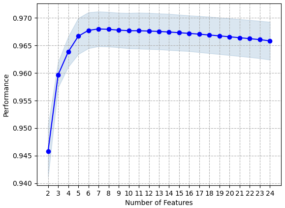
Figure A2 Sequential feature selection performance with 20 cross-validation steps, for the multiple linear regression at Hajala with the adjusted-R² as a function of the number of backward selected features, with 0.95 confidence interval.

Table A1 Variables used for the MLR model learning and inference for the Hajala and Col de Porte experiments.

Appendix B: Snow cover parameterization in cities

In cities, winter operations do not completely remove the snow cover. It remains for much longer on sideways or on car parks, and the excess snow on the road is gathered and packed at specific spots. This is particularly true in cold cities, subject to significant snowfall, with months of snow left over on the surfaces. While for road-focused simulations, the snow fraction is reset to 0 to model the complete removal of the snow cover on the road, this parameterization is incorrect at a city scale. Thus, the snow cover occupation is adapted here for urban environments.

We developed an option that modifies how the snow cover occupation is handled in the model. When a road maintenance operation occurs, snow cover is collected and stacked on a fraction of the total road surface. In the model, we call this fraction f_snstore. This parameter should then be representative of the remaining snow-covered surface fraction from the city snow removal operation procedure.

Between two snow removal operations, fresh snow, from new snowfall, accumulates. The prognostic fresh snow height variable D_fresh evolves as

$$\begin{array}{}\text{(B1)}& {\displaystyle }{\displaystyle \frac{\partial D_{\text{fresh}}}{\partial t}}={\displaystyle \frac{P_{\mathrm{n}}}{{\mathit{\rho }}_{\text{new}}}},\end{array}$$

with P_n the snow rate in ($\mathrm{kg}{\mathrm{m}}^{-\mathrm{2}}{\mathrm{s}}^{-\mathrm{1}}$) and ρ_new the fresh snow density in (kg m⁻³), as defined in Sect. 2.3. D_fresh is set to zero when the snow removal operations occur in the model, as it is then fully considered to be old snow.

This fresh snow is considered to fall first into the snow-covered area of the road, sidewalks, or car park, then to gradually cover the previously cleared roads and sidewalks, as shown in Fig. B1. The fresh snow occupation fraction is modelled as

$$\begin{array}{}\text{(B2)}& {\displaystyle }{\displaystyle }{f}_{\text{snfresh}}=min(\mathrm{1},max(D_{\text{fresh}}/\mathrm{0.01},f_{\text{snstore}}\left)\right).\end{array}$$

So, f_snfresh increases when the fresh snow cover exceeds the “old snow” cover.

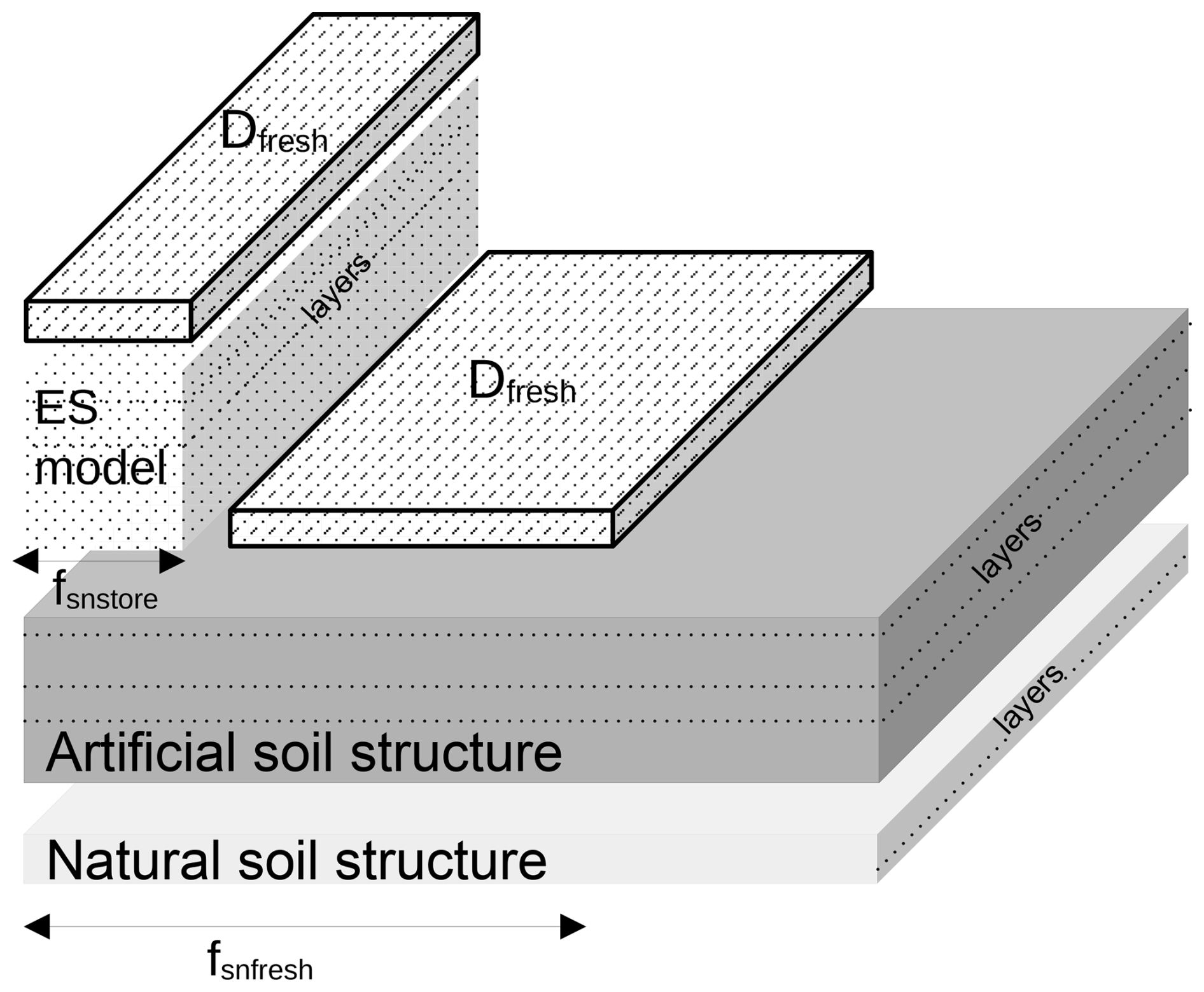
Figure B1 Schematic implementation of the new snow fraction procedure between two snow removal operations, as explained in the text when the fresh snow covers a fraction of the cleared road.

To parameterize the total occupation fraction of the snow cover, this fraction is compared with the total snow mantle depth D_s, which is the sum of the fresh snow and the piled up snow from the previous snow removal operation, used in Eq. 12. Thus, the new fraction is computed as

$$\begin{array}{}\text{(B3)}& {\displaystyle }& {\displaystyle }{f}_{\text{sn}}=min(min(\mathrm{1.0},D_{\mathrm{s}}/\mathrm{0.01}),f_{\text{snfresh}})⟺\text{(B4)}& {\displaystyle }& {\displaystyle }{f}_{\text{sn}}=min(\mathrm{1},D_{\mathrm{s}}/\mathrm{0.01},max(D_{\text{fresh}}/\mathrm{0.01},f_{\text{snstore}}\left)\right).\end{array}$$

This also means that during spring or even relatively warm situations in the cold season, when the total of the snow layer starts to completely melt, the fraction of snow will become smaller than the fraction of impervious surfaces assigned to store the old snow. This modelling is subject to an important assumption: for all computations linked to processes other than cover fraction on the impervious surfaces, the new fresh snow is considered to have the same properties and behaviour as the residual snow mantle. Thus, the evolution of the snow mantle is computed only once with the total snow height D_s, although the properties of the snow layer are not really horizontally homogeneous in the model tile considered.