Accounting for effects of coagulation and model uncertainties in particle number concentration estimates based on measurements from sampling lines – a Bayesian inversion approach with SLIC v1.0

The particle number (PN) emissions of both light- and heavy-duty vehicles are nowadays regulated and are typically measured from a full dilution tunnel with constant volume sampling (CVS). PN measurements for research and development purposes, though, are often taken from the raw exhaust to avoid the high setup costs of CVS. There is, however, a risk with these and any other kind of PN measurements with high number concentrations, which is that physical processes such as coagulation and diffusion losses inside sampling lines can alter, sometimes dramatically, the particle size distribution and bias its measurement. In this paper, we propose a method in the Bayesian framework for inverse problems to estimate the initial, unaltered particle size distribution based on the distorted measurements. The proposed method takes into account particle morphology and van der Waals and viscous forces in the coagulation model and allows the incorporation of prior information on the particle size distribution and, most importantly, a systematic quantification of uncertainty. We analyze raw exhaust PN measurements of a fuel-operated auxiliary heater and find that while a typical sampling line can reduce the PN by more than 50 %, the initial particle size distribution can be feasibly estimated with reasonable computational demands. The proposed method should give more freedom for designing the measurement setup and also aid in the comparison of results obtained at different sampling locations, such as CVS and tailpipe.

1 Introduction

Particulate matter (PM), i.e., particle pollution, poses great health risks to humans and causes environmental damage (Shiraiwa et al., 2017; Manisalidis et al., 2020). Significant PM sources, such as vehicle tailpipe emissions, are therefore in most cases subject to particle mass regulations and nowadays also to particle number (PN) regulations in Europe (Commission Regulation (EU), 2019; Giechaskiel et al., 2021b). PN regulations were introduced to better cover the fraction of ultrafine (<0.1 µm) particles, which is negligible in terms of mass but dominates the ambient atmosphere in terms of PN (80 %–90 % of all particles) (Hofman et al., 2016). These ultrafine particles are a cause of growing concern in the public health community due to their ability to circumvent primary airway defenses and penetrate deep in the lungs (Kwon et al., 2020; Morawska and Buonanno, 2021). Furthermore, the harmful systematic health effects associated with coarse (<10 µm) and fine (<2.5 µm) particulates can often be attributed to the fraction of ultrafine particles (Kwon et al., 2020). At the moment PN regulations are given for particles with a diameter >23 nm, not because smaller particles are any less dangerous, but mainly because smaller particles are very sensitive to sampling conditions and thus hard to measure accurately and with good repeatability (Giechaskiel et al., 2021b). The Euro 7 road vehicles emission standard proposal increases the size range to particles >10 nm (Giechaskiel et al., 2024). Details of the emissions such as those emitted from tailpipes are also important basic knowledge for the purpose of climate change research, as aerosol forcing uncertainty represents the largest climate forcing uncertainty overall (Kahn et al., 2023).

PN emissions are typically measured using condensation particle counters (e.g., Hering et al., 2005) or diffusion chargers (e.g., Schriefl et al., 2019), which can measure total PNs. If more detailed information is required, one can measure PN as a function of particle size, i.e., a particle size distribution (PSD), with an instrument such as the engine exhaust particle sizer (EEPS) spectrometer (TSI, 2024; Wang et al., 2016a). There are, however, aspects of PN measurement that may bias the results considerably unless explicitly accounted for in the design of the experiment (which may not always be possible) or numerically post-measurement. For example, measuring PSD in raw exhaust usually involves the use of sampling lines of different lengths to transfer and possibly cool the sample to the measurement devices. Within the sampling lines, the particles have a window of time to coagulate and diffuse onto the inner walls of the lines, which alters the PSD of the raw exhaust. The shortest possible residence times in the lines are typically targeted because residence times that are short enough (and PN concentrations low enough) limit the effects of diffusion and coagulation, leaving the PSD mostly unaltered. This may not always be practicable, however, and sometimes the PSD undergoes significant changes, up to more than an order of magnitude, especially in the concentrations of the smallest particle sizes. In one study, Giechaskiel et al. (2019) examined the measurement of PN directly from the tailpipe of heavy-duty engines and found that an increase from 0.5 to 4 m in the sampling line length resulted in a loss of 20 %–50 % of particles >10 nm, not explainable with just diffusion losses. Further, Liu et al. (2021) studied the effect of Brownian coagulation on particle evolution in gasoline engine exhaust by measuring the PSD at various locations along a laboratory exhaust system. They found that the PSD evolution mainly occurs for sizes <50 nm, that the evolution is dominated by coagulation, and that a significant (up to 90 %) particle reduction can occur when there is a high number of accumulation mode (>50 nm) particles. Such high losses would render a measurement useless unless the changes in the PSD are rigorously quantified and corrected for.

Of the physical processes in a sampling line, wall deposition losses are nowadays commonly corrected, but the effect of coagulation is typically not. Further, because the effect of coagulation is nonlinear and depends on the PN concentration, it cannot be corrected with a simple calibration measurement. To ensure coagulation and diffusion do not have a significant effect on the PSD, legislation specifies for example the maximum residence time and Reynolds number for a sample in the sampling line (Giechaskiel et al., 2021b), but we have not found in the literature attempts to correct the estimate of a PSD after the measurement has been made. In this paper, we aim to find out if the initial PSD can be estimated based on measurements that have been distorted by coagulation and diffusional losses. Our approach uses methods in the Bayesian framework for inverse problems (Kaipio and Somersalo, 2006) and makes use of a numerical model of the coagulation and wall diffusion process that takes into account the fractal nature of soot particles (Park et al., 2003; Rogak and Flagan, 1992) as well as van der Waals and viscous forces (Alam, 1987). Due to uncertainties related to the measurement (e.g., noise) and to the coagulation model (e.g., poorly known parameters), the resulting estimate is also uncertain to some degree. In the Bayesian framework, this uncertainty is quantified by the posterior probability density, i.e., the probability density of the unknown variable of interest, conditioned on the measurement. The possible prior information on the model unknown and statistics of the measurement noise are also accounted for. From the posterior one can calculate not only the most probable values of the initial PSD, but also the credible intervals to explicitly quantify the uncertainty of the PSD estimate. Robust uncertainty quantification is essential to assess the reproducibility of measurements between different laboratories (Giechaskiel et al., 2018, 2021a).

To test the proposed method, we carry out inversion with both synthetic data and real PSD measurements of a fuel-operated auxiliary heater (Oikarinen et al., 2022). We will compute the estimate of the initial PSD in two ways that are useful in different circumstances. The first one is based on solving an optimization problem, which is computationally fast and can be done in real time when collecting measurements in the field. In this case, the posterior uncertainty is approximated with a Gaussian distribution. The second approach is based on sampling the posterior with Markov chain Monte Carlo (MCMC), which is a lot more demanding computationally but does not need to rely on Gaussian approximations for the uncertainty estimates. The second approach can also be used to take into account the possible uncertainty in the parameters of the coagulation model, as will be shown later. We will also compare and discuss the results between the two approaches. The code and data used to carry out the examples in this paper are available in the package SLIC (Niskanen, 2024).

The remainder of the paper is organized as follows. In Sect. 2, we describe our approach to modeling coagulation and wall deposition. In Sect. 3, we describe and solve the inverse problem of estimating the initial PSD based on measurements done with a system that has a sampling line. In Sect. 4, we apply the method on synthetic and real data, and the results are discussed in Sect. 5. Finally, conclusions are given in Sect. 6.

2 Simulating the microphysical processes in a sampling line

When collecting PSD data from sampling lines, there are two main processes quick enough to affect aerosol particles during the short time (up to a few seconds) a sample resides in a sampling line: coagulation (agglomeration of particles) and wall deposition due to diffusion (particles lost to the sampling line walls). Together these processes reduce the number of particles and increase their size.

The time evolution of a PN concentration density n(v,t) (unit: ${\mathrm{m}}^{-\mathrm{1}}{\mathrm{cm}}^{-\mathrm{3}}$) experiencing coagulation and wall diffusion can be described by the following equation (Seinfeld and Pandis, 2016):

$$\begin{array}{ll}{\displaystyle \frac{\mathrm{d}n(v,t)}{\mathrm{d}t}}=& {\displaystyle }{\displaystyle \frac{\mathrm{1}}{\mathrm{2}}}\underset{\mathrm{0}}{\overset{v}{\int }}\mathit{\beta }(v-\overline{v},\overline{v})n(v-\overline{v},t)n(\overline{v},t)\mathrm{d}\overline{v}\\ \text{(1)}& {\displaystyle }& {\displaystyle }-n(v,t)\underset{\mathrm{0}}{\overset{\mathrm{\infty }}{\int }}\mathit{\beta }(\overline{v},v)n(\overline{v},t)\mathrm{d}\overline{v}-R\left(v\right)n(v,t),\end{array}$$

where the first integral represents a coagulation source, the second a coagulation sink, and R(v) in this case the rate of removal of particles by wall diffusion. Particle volume and time are denoted by v and t, respectively. The rate of coagulation is governed by the coagulation coefficient β(v₁,v₂), which describes the frequency that two particles of volume v₁ and v₂ collide.

To approximate the solution of Eq. (1) numerically, the particle size range is first discretized. We adopt here the sectional method (Gelbard et al., 1980; Jacobson et al., 1994; Lehtinen and Zachariah, 2001) for its computational efficiency and ease of implementation, where the particle size range is divided into a finite number of sections or bins. Here we use geometrically distributed bins so that the logarithm of the bin width is constant. The sectional method conserves total particle volume, and in Salminen et al. (2022) it was even found that for pure coagulation the sectional method can be more accurate than the finite element method with a similar number of discretization points.

In a typical implementation of the sectional method, particles within each bin are approximated to have a constant size equal to the bin middle point. Consider then two particles from bins with volumes v_i and v_j colliding and forming a larger particle with volume v_i+v_j. Unless the volume of the new particle coincides exactly with a center of a bin, the particle is divided into two adjacent bins in a way that conserves the total volume. For this purpose, let us define a size-splitting operator ξ_ijk, which gives the volume fraction of the coagulated particle v_i+v_j partitioned into bin k:

$$\begin{array}{}\text{(2)}& {\displaystyle }{\displaystyle }{\mathit{\xi }}_{ijk}=\left\{\begin{array}{ll}\frac{v_{k+\mathrm{1}}-(v_i+v_j)}{v_{k+\mathrm{1}}-v_k},& v_k\le v_i+v_j<v_{k+\mathrm{1}};k<n_{\mathrm{B}},\\ \mathrm{1}-{\mathit{\xi }}_{ij(k-\mathrm{1})},& v_{k-\mathrm{1}}<v_i+v_j<v_k;k>\mathrm{1},\\ \mathrm{1},& v_k\le v_i+v_j;k=n_{\mathrm{B}},\\ \mathrm{0},& \text{otherwise},\end{array}\right.\end{array}$$

where n_B is the total number of bins. Let us now denote the PN concentration in the kth bin by N_k=n_kΔD_p, where ΔD_p is the width and n_k the PN concentration density (cf. n(v,t) in Eq. 1) of bin k and $k=\mathrm{1},\mathrm{\dots },n_{\mathrm{B}}$. The discretized version of Eq. (1) then reads

$$\begin{array}{}\text{(3)}& {\displaystyle }{\displaystyle \frac{\mathrm{d}{N}_k}{\mathrm{d}t}}={\displaystyle \frac{\mathrm{1}}{\mathrm{2}}}\sum _{i,j}{\mathit{\xi }}_{ijk}{\mathit{\beta }}_{ij}{N}_i{N}_j-\sum _i{\mathit{\beta }}_{ik}{N}_i{N}_k-R_k{N}_k,\end{array}$$

where β_ij is the coagulation coefficient between size bins i and j. Time integration for Eq. (3) can be carried out for example with Runge–Kutta methods. We use here RK45 as implemented in SciPy (Virtanen et al., 2020).

2.1 Coagulation model

Particles collide due to their Brownian, or thermal, motion, as well as motion due to external forces such as laminar shear or turbulent flow and gravitational, van der Waals, Coulomb, and hydrodynamic forces (Seinfeld and Pandis, 2016). Colliding liquid particles coalesce and retain their spherical shape. Solid particles above a certain critical size r₁, however, are not expected to coalesce but instead form fractal-like agglomerates of dense primary particles. The collision frequency for fractal-like particles can be significantly higher than for spherical particles with the same volume (Rogak and Flagan, 1992).

In this work, for coagulation we consider the particles' Brownian motion and the effects of van der Waals and viscous forces, as those are likely to dominate over other factors in coagulation at short timescales and distances. Further, in our specific example with soot particles, we will take into account the particle shape because soot particles are known to form long chains of aerosol agglomerates (Park et al., 2003). Figure 1 demonstrates the effect of fractal geometry and van der Waals and viscous forces on the coagulation coefficient. Although other aspects of coagulation such as the effect of charge or turbulent flow are not modeled in this work, they can be included in the considered framework should the need arise. For examples that have dealt with the Coulombic effects see Mahfouz and Donahue (2021a), Mahfouz and Donahue (2021b), Pfeifer et al. (2023), and Thomas et al. (2024), and for examples on the effect of turbulence see Okuyama et al. (1978), Williams and Crane (1983), and Zhao et al. (2021).

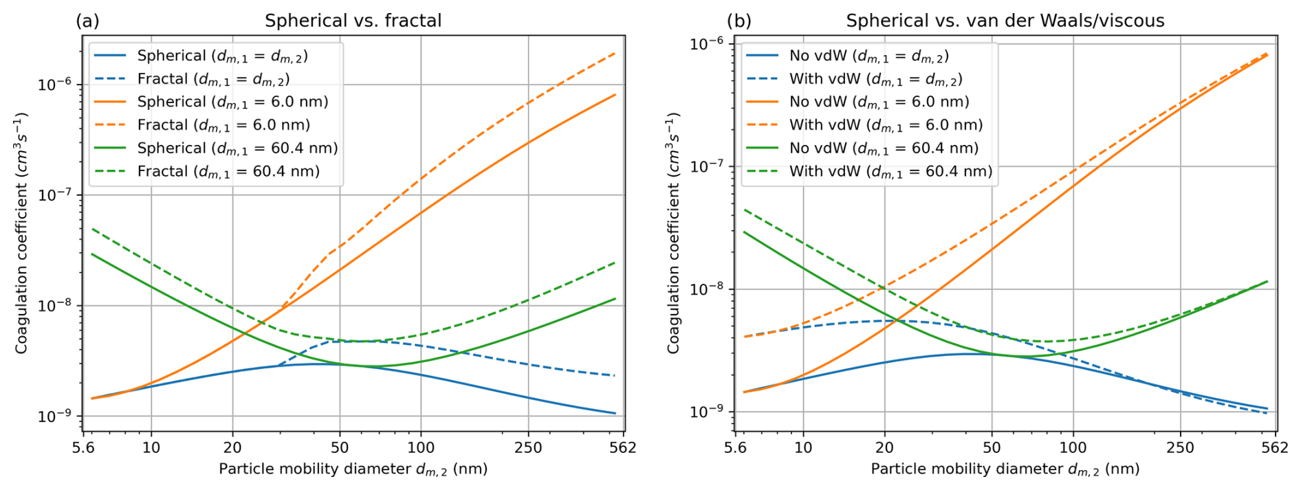
Figure 1 Coagulation coefficients calculated for mobility diameters 5.62–562 nm. (a) Spherical vs. fractal coagulation coefficient (fractal dimension =1.7 and primary particle diameter =30 nm). (b) Spherical coagulation coefficient with and without van der Waals and viscous forces (Hamaker constant $=\mathrm{2}\times {\mathrm{10}}^{-\mathrm{19}}$ J).

2.1.1 Brownian coagulation of fractal-like agglomerates

In this paper, the coagulation of fractal-like agglomerates is modeled following mostly Rogak and Flagan (1992) and Jacobson and Seinfeld (2004), where it is assumed that the agglomerate structure is completely determined by three parameters: the fractal dimension D_f, the primary particle radius r₁, and the number of primary particles 𝒩. All primary particles are thus assumed to be of the same size. The fractal dimension, $D_{\mathrm{f}}\in [\mathrm{1},\mathrm{3}]$, characterizes the shape of the agglomerate. For example, when D_f=1, the agglomerate forms a line, whereas with D_f=2, it fills space like a surface, and as D_f approaches 3, it curls up to resemble a spherical volume. For soot particles, typical values for the primary particle radius are between 10 and 17 nm and the fractal dimension between 1.5 and 2.2 (Wentzel et al., 2003; Lapuerta et al., 2017).

The three parameters above give rise to a number of equivalent radii that characterize the coagulation of non-spherical particles. Let us first highlight two here: the volume equivalent radius and the mobility radius. The volume equivalent radius, r_v, is the radius of a sphere with the same volume as the aggregate, whereas the mobility radius, r_m, is the radius of a sphere that experiences the same drag force as the agglomerate under the same dynamic conditions (Rogak and Flagan, 1992). This distinction is important, because while mobility radii are what is usually measured, the size-splitting coefficient Eq. (2) should be calculated using the volume equivalent radii to conserve particle volume. Thus, for non-spherical particles, the output bin sizes of a typical measurement device should not be used directly for modeling coagulation.

Let us first state 𝒩_i as the ratio of the volumes of the aggregate and the primary particle, ${\mathcal{N}}_i=(r_{\mathrm{v},i}/r_{\mathrm{1}}{)}^{\mathrm{3}}$, where i refers to the index of a size bin. The fractal or outer radius of the agglomerate is then defined as

$$\begin{array}{}\text{(4)}& {\displaystyle }{\displaystyle }{r}_{\mathrm{f},i}=\left\{\begin{array}{ll}{r}_{\mathrm{1}}{\mathcal{N}}_i^{\mathrm{1}/D_{\mathrm{f}}},& r_{\mathrm{v},i}\ge r_{\mathrm{1}},\\ r_{\mathrm{v},i},& r_{\mathrm{v},i}<r_{\mathrm{1}}.\end{array}\right.\end{array}$$

The Brownian coagulation rate between two particles of sizes i and j can be stated in the Fuchs form, modified for fractal geometry, as

$$\begin{array}{}\text{(5)}& {\displaystyle }{\displaystyle }{\mathit{\beta }}_{i,j}=\mathrm{4}\mathit{\pi }(r_{\mathrm{c},i}+r_{\mathrm{c},j})(D_{\mathrm{m},i}+D_{\mathrm{m},j})C_{i,j}^{-\mathrm{1}},\end{array}$$

where r_c,i and D_m,i are the collision radius and Brownian diffusion coefficient of particle i, respectively, and C_i,j is a transition-regime correction factor that extends the validity of the formula from the continuum regime to sizes smaller or comparable to the mean free path of diffusion particles. Following Rogak and Flagan (1992), we set the collision radius equal to the outer radius of the particle, $r_{\mathrm{c},i}=r_{\mathrm{f},i}$.

The expressions for D_m,i and C_i,j require the (transition-regime) mobility radius r_m,i, which is computed by interpolating between the continuum-regime mobility radius r_mc,i and free-molecular-regime mobility radius r_mk,i, as

$$\begin{array}{}\text{(6)}& {\displaystyle }{\displaystyle \frac{r_{\mathrm{m},i}}{C_{\mathrm{c}}\left({\mathit{\text{Kn}}}_{\mathrm{m},i}\right)}}={\displaystyle \frac{r_{\text{mc},i}}{C_{\mathrm{c}}\left({\mathit{\text{Kn}}}_{\mathrm{a},i}\right)}},\end{array}$$

where C_c(Kn) is the Cunningham slip correction factor, given by

$$\begin{array}{}\text{(7)}& {\displaystyle }{\displaystyle }{C}_{\mathrm{c}}\left(\mathit{\text{Kn}}\right)=\mathrm{1}+\mathit{\text{Kn}}(\mathrm{1.257}+\mathrm{0.4}\exp (-\mathrm{1.1}/\mathit{\text{Kn}}\left)\right),\end{array}$$

with Kn representing the Knudsen number. The mobility radius Knudsen number is given by

$$\begin{array}{}\text{(8)}& {\mathit{\text{Kn}}}_{\mathrm{m},i}={\displaystyle \frac{{\mathit{\lambda }}_{\mathrm{a}}}{r_{\mathrm{m},i}}}\end{array}$$

and the adjusted Knudsen number by

$$\begin{array}{}\text{(9)}& {\mathit{\text{Kn}}}_{\mathrm{a},i}={\displaystyle \frac{{\mathit{\lambda }}_{\mathrm{a}}{r}_{\text{mc},i}}{r_{\text{mk},i}^{\mathrm{2}}}}.\end{array}$$

Above, λ_a denotes the mean free path of an air molecule, which can be calculated from

$$\begin{array}{}\text{(10)}& {\displaystyle }{\displaystyle }{\mathit{\lambda }}_{\mathrm{a}}={\displaystyle \frac{k_{\mathrm{B}}T}{\sqrt{\mathrm{2}}\mathit{\pi }{d}^{\mathrm{2}}p}},\end{array}$$

where k_B is the Boltzmann constant, T is the gas temperature, d is the diameter of an air molecule (approximated here as the diameter of a nitrogen molecule), and p is the gas pressure. The free-molecular-regime mobility radius, r_mk,i, is assumed to be equal to the projected-area equivalent radius r_A,i, given by

$$\begin{array}{}\text{(11)}& {\displaystyle }{\displaystyle }{r}_{\mathrm{A},i}=\left\{\begin{array}{l}{r}_{\mathrm{1}}\sqrt{max\mathit{\{}{N}_i^{\mathrm{2}/\mathrm{3}},min[\begin{array}{l}\mathrm{1}+\mathrm{0.67}(N_i-\mathrm{1}),\\ D_{\mathrm{f}}{N}_i^{\mathrm{2}/D_{\mathrm{f}}}/\mathrm{3}\end{array}\left]\mathit{\right\}}},\\ r_{\mathrm{v},i}\ge r_{\mathrm{1}},\\ r_{\mathrm{v},i},r_{\mathrm{v},i}<r_{\mathrm{1}},\end{array}\right.\end{array}$$

and the continuum-regime mobility radius is given by

$$\begin{array}{}\text{(12)}& {\displaystyle }{\displaystyle }{r}_{\text{mc},i}=max\left\{\begin{array}{l}{r}_{\mathrm{f},i}{\left[\ln \left(\mathrm{2}\frac{r_{\mathrm{f},i}}{r_{\mathrm{1}}}\right)+\mathrm{1}\right]}^{-\mathrm{1}},\\ r_{\mathrm{f},i}{\left(\frac{D_{\mathrm{f}}-\mathrm{1}}{\mathrm{2}}\right)}^{\mathrm{0.7}},r_{\mathrm{A},i}\end{array}\right\}.\end{array}$$

Now, the diffusion coefficient can be calculated from

$$\begin{array}{}\text{(13)}& {\displaystyle }{\displaystyle }{D}_{\mathrm{m},i}={\displaystyle \frac{k_{\mathrm{B}}T}{\mathrm{6}\mathit{\pi }\mathit{\eta }{r}_{\mathrm{m},i}}}{C}_{\mathrm{c}}\left({\mathit{\text{Kn}}}_{\mathrm{m},i}\right),\end{array}$$

where η represents the dynamic viscosity of gas, which is temperature-dependent and over the range of 100–1800 K can be determined using the Sutherland equation (Hinds, 1999):

$$\begin{array}{}\text{(14)}& {\displaystyle }{\displaystyle }\mathit{\eta }={\displaystyle \frac{\mathrm{1.458}\times {\mathrm{10}}^{-\mathrm{6}}\text{Pa}\cdot \mathrm{s}\cdot \mathrm{K}{\left(\frac{T}{\mathrm{K}}\right)}^{\mathrm{1.5}}}{T+\mathrm{110.4}\mathrm{K}}}.\end{array}$$

The correction factor C_i,j is given by

$$\begin{array}{}\text{(15)}& {\displaystyle }{\displaystyle }{C}_{i,j}={\displaystyle \frac{r_{\mathrm{c},i}+r_{\mathrm{c},j}}{r_{\mathrm{c},i}+r_{\mathrm{c},j}+\sqrt{{\mathit{\delta }}_{\mathrm{m},i}^{\mathrm{2}}+{\mathit{\delta }}_{\mathrm{m},j}^{\mathrm{2}}}}}+\stackrel{\mathrm{̃}}{c},\end{array}$$

where

$$\begin{array}{}\text{(16)}& {\displaystyle }{\displaystyle }{\mathit{\delta }}_{\mathrm{m},i}={\displaystyle \frac{(\mathrm{2}{r}_{\mathrm{m},i}+{\mathit{\lambda }}_{\mathrm{m},i}{)}^{\mathrm{3}}-(\mathrm{4}{r}_{\mathrm{m},i}^{\mathrm{2}}+{\mathit{\lambda }}_{\mathrm{m},i}^{\mathrm{2}}{)}^{\mathrm{3}/\mathrm{2}}}{\mathrm{6}{r}_{\mathrm{m},i}{\mathit{\lambda }}_{\mathrm{m},i}}}-\mathrm{2}{r}_{\mathrm{m},i}\end{array}$$

and

$$\begin{array}{}\text{(17)}& {\displaystyle }{\displaystyle }\stackrel{\mathrm{̃}}{c}={\displaystyle \frac{\mathrm{4}(D_{\mathrm{m},i}+D_{\mathrm{m},j})}{\sqrt{{\overline{v}}_i^{\mathrm{2}}+{\overline{v}}_j^{\mathrm{2}}}(r_{\mathrm{c},i}+r_{\mathrm{c},j})}}.\end{array}$$

The effective mean free path of a particle size i is given by

$$\begin{array}{}\text{(18)}& {\displaystyle }{\displaystyle }{\mathit{\lambda }}_{\mathrm{m},i}={\displaystyle \frac{\mathrm{8}{D}_{\mathrm{m},i}}{\mathit{\pi }{\overline{v}}_i}},\end{array}$$

with the mean thermal speed

$$\begin{array}{}\text{(19)}& {\displaystyle }{\displaystyle }{\overline{v}}_i=\sqrt{{\displaystyle \frac{\mathrm{8}{k}_{\mathrm{B}}T}{\mathit{\pi }{\overline{M}}_i}}},\end{array}$$

where ${\overline{M}}_i=\mathrm{4}/\mathrm{3}\mathit{\pi }{r}_{\mathrm{v},i}^{\mathrm{3}}\mathit{\rho }$ is the mass of a single particle, with ρ denoting the particle density.

The above model was written in terms of the volume equivalent radius r_v and parameters D_f and r₁ to find the mobility radius r_m; i.e., it forms a relation $f:r_{\mathrm{v}}\mapsto r_{\mathrm{m}}$. On the other hand, measurements of PN concentration are usually modeled with respect to r_m, and hence, a mapping from r_m to r_v is needed. An explicit solution $f^{-\mathrm{1}}:r_{\mathrm{m}}\mapsto r_{\mathrm{v}}$ is not possible, though, and we calculate r_v by solving a minimization problem:

$$\begin{array}{}\text{(20)}& {\displaystyle }{\displaystyle }{r}_{\mathrm{v},i}=\arg \underset{r_{\mathrm{v},i}}{min}\Vert r_{\mathrm{m},i}-f(r_{\mathrm{v},i},r_{\mathrm{1}},D_{\mathrm{f}}){\Vert }_{\mathrm{2}}^{\mathrm{2}}.\end{array}$$

2.1.2 Van der Waals and viscous forces

Van der Waals forces are weak fluctuating dipole–dipole forces that increase the rate of aerosol coagulation (Alam, 1987). Viscous forces, on the other hand, slow down the rate of coagulation. Viscous forces are absent in the free molecular regime but in the continuum regime can even slow down coagulation more than van der Waals forces enhance it (Jacobson and Seinfeld, 2004). These forces can be taken into account by multiplying the Brownian coagulation coefficient Eq. (5) by a correction factor V_i,j. We follow here Alam (1987), who determined an interpolation formula for the correction factor between the free-molecular and continuum regimes as

$$\begin{array}{}\text{(21)}& {\displaystyle }{\displaystyle }{V}_{i,j}={\displaystyle \frac{W_{\mathrm{c},i,j}\left[\mathrm{1}+\stackrel{\mathrm{̃}}{c}\right]}{\mathrm{1}+W_{\mathrm{c},i,j}/W_{\mathrm{k},i,j}\stackrel{\mathrm{̃}}{c}}},\end{array}$$

where $\stackrel{\mathrm{̃}}{c}$ is defined in Eq. (17) and $W_{\mathrm{k},i,j}$ and $W_{\mathrm{c},i,j}$ are correction factors for the free-molecular and continuum regimes, respectively. These are given by

$$\begin{array}{ll}{\displaystyle }{W}_{\mathrm{k},i,j}=& {\displaystyle }{\displaystyle \frac{-\mathrm{1}}{\mathrm{2}(r_i+r_j{)}^{\mathrm{2}}{k}_{\mathrm{B}}T}}\\ {\displaystyle }& {\displaystyle }\times \underset{r_i+r_j}{\overset{\mathrm{\infty }}{\int }}\left({\displaystyle \frac{\mathrm{d}{E}_{i,j}\left(r\right)}{\mathrm{d}r}}+r{\displaystyle \frac{{\mathrm{d}}^{\mathrm{2}}{E}_{i,j}\left(r\right)}{\mathrm{d}{r}^{\mathrm{2}}}}\right)\\ \text{(22)}& {\displaystyle }& {\displaystyle }\times \exp \left[{\displaystyle \frac{-\mathrm{1}}{k_{\mathrm{B}}T}}\left({\displaystyle \frac{r}{\mathrm{2}}}{\displaystyle \frac{\mathrm{d}{E}_{i,j}\left(r\right)}{\mathrm{d}r}}+E_{i,j}\left(r\right)\right)\right]r^{\mathrm{2}}\mathrm{d}r\end{array}$$

and

$$\begin{array}{ll}{\displaystyle }{W}_{\mathrm{c},i,j}=[& {\displaystyle }(r_i+r_j)\\ \text{(23)}& {\displaystyle }& {\displaystyle }\times \underset{r_i+r_j}{\overset{\mathrm{\infty }}{\int }}{\displaystyle \frac{D^{\mathrm{\infty }}}{D_{i,j}}}\left(r\right)\exp \left({\displaystyle \frac{E_{i,j}\left(r\right)}{k_{\mathrm{B}}T}}\right){\displaystyle \frac{\mathrm{d}r}{r^{\mathrm{2}}}}{]}^{-\mathrm{1}}.\end{array}$$

The correction factors include the Van der Waals interaction potential

$$\begin{array}{ll}{\displaystyle }{E}_{i,j}\left(r\right)=& {\displaystyle }-{\displaystyle \frac{A}{\mathrm{6}}}[{\displaystyle \frac{\mathrm{2}{r}_i{r}_j}{r^{\mathrm{2}}-(r_i+r_j{)}^{\mathrm{2}}}}+{\displaystyle \frac{\mathrm{2}{r}_i{r}_j}{r^{\mathrm{2}}-(r_i-r_j{)}^{\mathrm{2}}}}\\ \text{(24)}& {\displaystyle }& {\displaystyle }+\ln {\displaystyle \frac{r^{\mathrm{2}}-(r_i+r_j{)}^{\mathrm{2}}}{r^{\mathrm{2}}-(r_i-r_j{)}^{\mathrm{2}}}}],\end{array}$$

where A is the Hamaker constant, and the diffusion ratio that corrects the diffusion coefficient in the continuum regime for viscous forces

$$\begin{array}{ll}{\displaystyle \frac{D^{\mathrm{\infty }}}{D_{i,j}}}\left(r\right)=& {\displaystyle }\mathrm{1}+{\displaystyle \frac{\mathrm{2.6}{r}_i{r}_j}{(r_i+r_j{)}^{\mathrm{2}}}}\sqrt{{\displaystyle \frac{r_i{r}_j}{(r_i+r_j)(r-r_i-r_j)}}}\\ \text{(25)}& {\displaystyle }& {\displaystyle }+{\displaystyle \frac{r_i{r}_j}{(r_i+r_j)(r-r_i-r_j)}}.\end{array}$$

Typical values for the Hamaker constant of soot are in the range of $\mathrm{1}\times {\mathrm{10}}^{-\mathrm{19}}$–$\mathrm{4}\times {\mathrm{10}}^{-\mathrm{19}}$ J (Liu et al., 2018).

2.2 Wall deposition by diffusion

Aerosol particles adhere when they collide with a surface, and thus their concentration at the surface is zero. This results in a concentration gradient near the surface which causes a continuous diffusion of particles to the surface. In addition to diffusion, other basic mechanisms of wall deposition include electrostatic attraction, i.e., the effect of charges on the walls (Mahfouz and Donahue, 2020); inertial impaction; interception; and gravitational settling (Hinds, 1999). Also surface properties such as roughness can influence deposition (Shimada et al., 1987; Hussein et al., 2012). In this paper, we only model wall deposition by diffusion, but other mechanisms can naturally be included in the model as needed.

For laminar flow of particles through a cylindrical tube, the fraction $P=n_{\text{out}}/n_{\text{in}}$ of entering particles that exit as a result of diffusional losses can be approximated with the help of a dimensionless diffusion parameter μ as (Hinds, 1999)

$$\begin{array}{}\text{(26)}& {\displaystyle }{\displaystyle }P=\left\{\begin{array}{ll}\mathrm{1}-\mathrm{5.50}{\mathit{\mu }}^{\mathrm{2}/\mathrm{3}}+\mathrm{3.77}\mathit{\mu },& \mathit{\mu }<\mathrm{0.009},\\ \mathrm{0.819}\exp (-\mathrm{11.5}\mathit{\mu })& \\ +\mathrm{0.0957}\exp (-\mathrm{70.1}\mathit{\mu }),& \mathit{\mu }\ge \mathrm{0.009}.\end{array}\right.\end{array}$$

The diffusion parameter is defined as

$$\begin{array}{}\text{(27)}& {\displaystyle }{\displaystyle }\mathit{\mu }={\displaystyle \frac{DL}{Q}},\end{array}$$

where L is the tube length and Q is the volume flow rate (m³ s⁻¹) through the tube. For the particle diffusion coefficient D we use D_m from Eq. (13). To transform the penetration P into the removal term R in Eq. (3), we set

$$\begin{array}{}\text{(28)}& {\displaystyle }{\displaystyle }R=-\log \left(P\right)/T,\end{array}$$

where T is the residence time of the aerosol in the tube.

3 Estimating the initial size distribution

Let us now formulate the problem of estimating the initial PSD as a problem of statistical inference within the Bayesian framework. The unknown parameters are modeled as random variables, and all information on them is expressed in terms of probability density functions. The solution to the inference problem is the posterior probability density, a conditional probability density of the unknown parameters conditioned on the measured data (Kaipio and Somersalo, 2006).

Let us denote by $\stackrel{\mathrm{̃}}{\mathit{N}}\in {\mathbb{R}}^{n_{\mathrm{B}}}$ a vector of length n_B that represents a parametrization of the PSD of the aerosol at the entry of the sampling line (i.e., the initial PSD). This will be the model unknown in the Bayesian inference. In the parametrization used below, $\stackrel{\mathrm{̃}}{\mathit{N}}$ consists of the logarithms of the size-discretized PSD $\mathit{N},\stackrel{\mathrm{̃}}{\mathit{N}}:=\log \mathit{N}$, to enforce positivity and to treat the wide range of number concentrations in a numerically more stable way. In what follows, $\stackrel{\mathrm{̃}}{\cdot }$ will be used to denote a variable on the log scale. Further, let $\mathit{y}\in {\mathbb{R}}^{n_M}$ be a vector of length n_M consisting of noisy, indirect observations of the PSD after the particles have undergone coagulation and diffusion processes when transported through the sampling line. The posterior is then given by Bayes' formula,

$$\begin{array}{}\text{(29)}& {\displaystyle }{\displaystyle }\mathit{\pi }\left(\stackrel{\mathrm{̃}}{\mathit{N}}\right|\mathit{y})={\displaystyle \frac{\mathit{\pi }\left(\mathit{y}\right|\stackrel{\mathrm{̃}}{\mathit{N}}\left)\mathit{\pi }\right(\stackrel{\mathrm{̃}}{\mathit{N}})}{\mathit{\pi }\left(\mathit{y}\right)}}\propto \mathit{\pi }(\mathit{y}\left|\stackrel{\mathrm{̃}}{\mathit{N}}\right)\mathit{\pi }\left(\stackrel{\mathrm{̃}}{\mathit{N}}\right),\end{array}$$

where $\mathit{\pi }\left(\mathit{y}\right|\stackrel{\mathrm{̃}}{\mathit{N}})$ is the likelihood function; $\mathit{\pi }\left(\stackrel{\mathrm{̃}}{\mathit{N}}\right)$ is the prior probability density; and π(y) is the value of the marginal probability density of measurements at y, which once the measurements are realized, acts as a normalization constant. The likelihood function describes the likelihood of different measurement outcomes given a realization of parameters $\stackrel{\mathrm{̃}}{\mathit{N}}$. It considers statistics of the measurement noise and the misfit between measurements and the model. The prior density models statistically the information on the parameters before measurements y are accounted for. It should include a higher probability for parameter values we expect to see compared to those we do not expect to see, and can, for example, include an assumption that small differences in number concentration between neighboring size bins are more probable than large ones.

3.1 The prior

We model the prior density as Gaussian with mean ${\stackrel{\mathrm{̃}}{\mathit{N}}}_{*}$ and covariance ${\stackrel{\mathrm{̃}}{\mathbf{\Gamma }}}_{\text{pr}}$. The covariance is constructed to promote smoothness (Lieberman et al., 2010) between adjacent size bins:

$$\begin{array}{}\text{(30)}& {\displaystyle }{\displaystyle }{\stackrel{\mathrm{̃}}{\mathbf{\Gamma }}}_{\text{pr}}(i,j)=\stackrel{\mathrm{̃}}{a}\exp \left\{-{\displaystyle \frac{\mathrm{1}}{\mathrm{2}}}{\displaystyle \frac{\Vert {\stackrel{\mathrm{̃}}{d}}_i-{\stackrel{\mathrm{̃}}{d}}_j{\Vert }^{\mathrm{2}}}{{\stackrel{\mathrm{̃}}{b}}^{\mathrm{2}}}}\right\},\end{array}$$

where $\stackrel{\mathrm{̃}}{a}={\stackrel{\mathrm{̃}}{\mathbf{\Gamma }}}_{\text{pr}}(i,i)$ is the variance of the initial PSD, ${\stackrel{\mathrm{̃}}{d}}_i$ is the size bin center, and $\stackrel{\mathrm{̃}}{b}=\stackrel{\mathrm{̃}}{l}/\sqrt{\mathrm{2}\ln \left(\mathrm{100}\right)}$ is related to the smoothness of the initial PSD over the size range. The degree of smoothness is controlled by correlation length $\stackrel{\mathrm{̃}}{l}$, which is defined as the distance (here, in terms of particle size on a logarithmic scale) over which the cross-covariance ${\stackrel{\mathrm{̃}}{\mathbf{\Gamma }}}_{\text{pr}}(i,j)$ drops to 1 % of $\stackrel{\mathrm{̃}}{a}$. Due to the log transformation, a correlation length $\stackrel{\mathrm{̃}}{l}=\mathrm{1}$ corresponds to 1 order of magnitude. An example of a covariance matrix with $\stackrel{\mathrm{̃}}{l}=\mathrm{3}/\mathrm{4}$ and $\stackrel{\mathrm{̃}}{a}=\mathrm{4}$, when each order of magnitude is divided into 16 bins, is shown in Fig. 2.

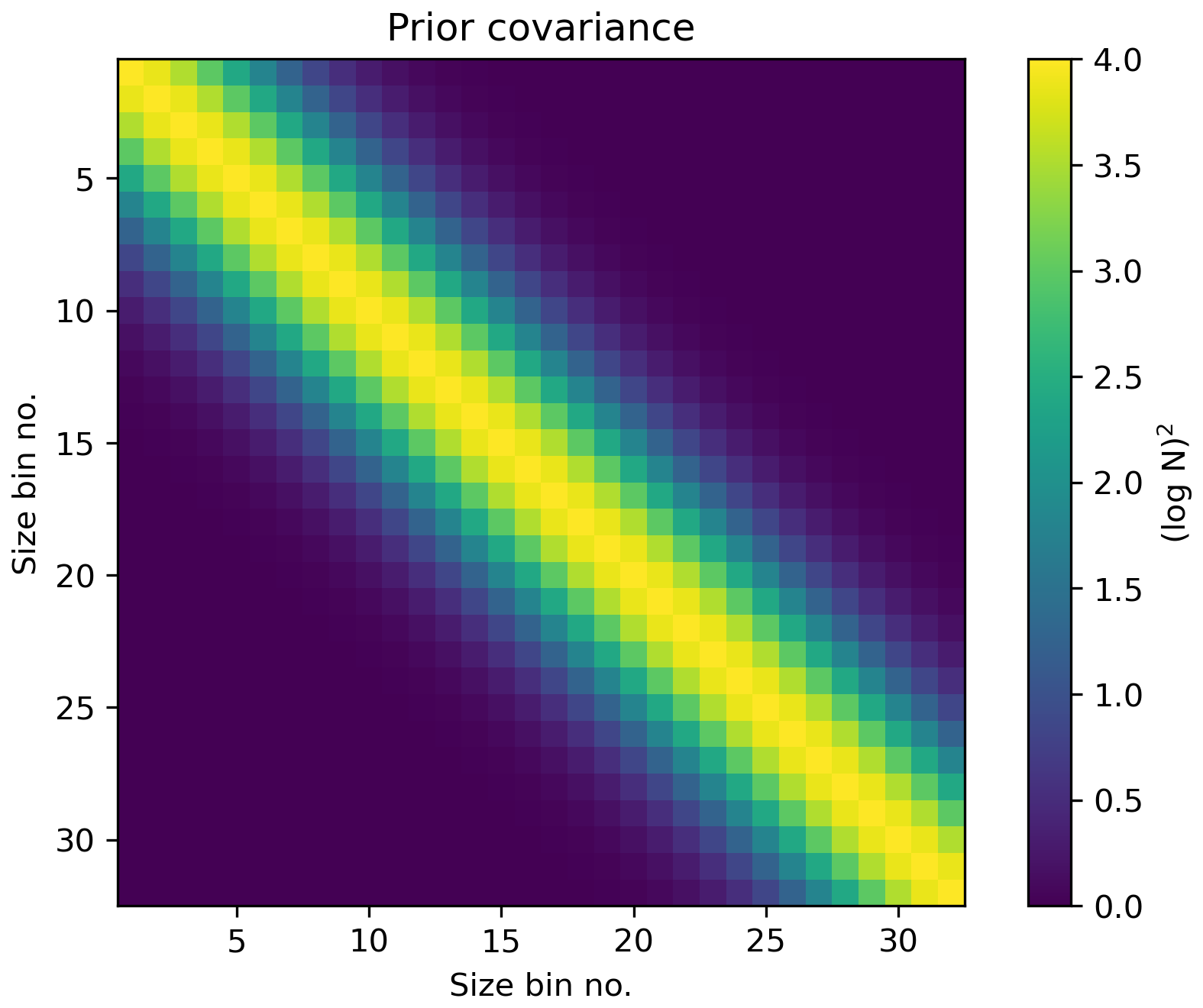
Figure 2 An example prior covariance matrix with size bins covering 2 orders of magnitude and 16 bins per decade.

With the above notation, the prior density can be written as

$$\begin{array}{}\text{(31)}& {\displaystyle }{\displaystyle }\mathit{\pi }\left(\stackrel{\mathrm{̃}}{\mathit{N}}\right)\propto \exp \left\{-{\displaystyle \frac{\mathrm{1}}{\mathrm{2}}}{∥{\stackrel{\mathrm{̃}}{\mathbf{L}}}_{\text{pr}}\left({\stackrel{\mathrm{̃}}{\mathit{N}}}_{*}-\stackrel{\mathrm{̃}}{\mathit{N}}\right)∥}^{\mathrm{2}}\right\},\end{array}$$

where ${\stackrel{\mathrm{̃}}{\mathbf{L}}}_{\text{pr}}$ is a matrix square root of the inverse of the prior covariance, i.e., ${\stackrel{\mathrm{̃}}{\mathbf{L}}}_{\text{pr}}^{\mathrm{T}}{\stackrel{\mathrm{̃}}{\mathbf{L}}}_{\text{pr}}={\stackrel{\mathrm{̃}}{\mathbf{\Gamma }}}_{\text{pr}}^{-\mathrm{1}}$.

3.2 The likelihood

Let $h:{\mathbb{R}}^{n_{\mathrm{B}}}\to {\mathbb{R}}^{n_M}$ denote the parameter-to-observable mapping, i.e., the forward model, which models the dependency between the initial time PSD (or, to be specific, its logarithmic parameters) and the observable quantity; i.e., in this case, h models not only the measurement device but also the coagulation and wall deposition processes that the particle ensemble undergoes while being transported through the sampling line between the initial time and the time of the observation. We will derive the exact form of h in Sect. 4 because it depends on the measurement device used. With the standard assumption that the measurement process is corrupted by additive Gaussian noise $\mathit{e}\in {\mathbb{R}}^{n_M}$, the following observation model can be written for the measurement:

$$\begin{array}{}\text{(32)}& {\displaystyle }{\displaystyle }\mathit{y}=h\left(\stackrel{\mathrm{̃}}{\mathit{N}}\right)+\mathit{e}.\end{array}$$

If we assume that the measurement noise is independent of the unknowns and normally distributed with zero mean and covariance ${\mathbf{\Gamma }}_{\mathrm{e}},\mathit{e}\sim \mathcal{N}(\mathrm{0},{\mathbf{\Gamma }}_{\mathrm{e}})$, the likelihood can be written as

$$\begin{array}{}\text{(33)}& {\displaystyle }{\displaystyle }\mathit{\pi }\left(\mathit{y}\right|\stackrel{\mathrm{̃}}{\mathit{N}})\propto \exp \left\{-{\displaystyle \frac{\mathrm{1}}{\mathrm{2}}}{∥{\mathbf{L}}_{\mathrm{e}}\left(\mathit{y}-h\left(\stackrel{\mathrm{̃}}{\mathit{N}}\right)\right)∥}^{\mathrm{2}}\right\},\end{array}$$

where ${\mathbf{L}}_{\mathrm{e}}^{\mathrm{T}}{\mathbf{L}}_{\mathrm{e}}={\mathbf{\Gamma }}_{\mathrm{e}}^{-\mathrm{1}}$.

3.3 The posterior

The solution to the inference problem, the posterior density Eq. (29), can now be stated by combining the prior Eq. (31) and the likelihood Eq. (33):

$$\begin{array}{ll}{\displaystyle }\mathit{\pi }\left(\stackrel{\mathrm{̃}}{\mathit{N}}\right|\mathit{y})\propto & {\displaystyle }\exp \mathit{\{}-{\displaystyle \frac{\mathrm{1}}{\mathrm{2}}}{∥{\mathbf{L}}_{\mathrm{e}}(\mathit{y}-h(\stackrel{\mathrm{̃}}{\mathit{N}}\left)\right)∥}^{\mathrm{2}}\\ \text{(34)}& {\displaystyle }& {\displaystyle }-{\displaystyle \frac{\mathrm{1}}{\mathrm{2}}}{∥{\mathbf{L}}_{\text{pr}}({\stackrel{\mathrm{̃}}{\mathit{N}}}_{*}-\stackrel{\mathrm{̃}}{\mathit{N}})∥}^{\mathrm{2}}\mathit{\}}.\end{array}$$

The final task in the problem is to summarize the posterior by calculating point and interval estimates, which we will describe next.

3.3.1 Laplace approximation to the posterior

One of the most commonly used approximations to the posterior is the Laplace approximation, in which the posterior density is approximated with a Gaussian distribution (MacKay, 2003). The mean of the distribution is set to the maximum a posteriori (MAP) estimate, and the covariance is calculated based on the curvature of the posterior around the MAP estimate, i.e., $\mathit{\pi }\left(\stackrel{\mathrm{̃}}{\mathit{N}}\right|\mathit{y})\approx \mathcal{N}({\stackrel{\mathrm{̃}}{\mathit{N}}}_{\text{MAP}},{\stackrel{\mathrm{̃}}{\mathbf{\Gamma }}}_{\text{post}})$. The MAP estimate is defined as the point where the posterior density has a maximum:

$$\begin{array}{}\text{(35)}& {\displaystyle }{\displaystyle }{\stackrel{\mathrm{̃}}{\mathit{N}}}_{\text{MAP}}=\underset{\stackrel{\mathrm{̃}}{\mathit{N}}\in \mathcal{D}}{\arg max}\mathit{\pi }\left(\stackrel{\mathrm{̃}}{\mathit{N}}\right|\mathit{y}),\end{array}$$

where $\mathcal{D}\subset {\mathbb{R}}^{n_{\mathrm{B}}}$ is a space of possible values for $\stackrel{\mathrm{̃}}{\mathit{N}}$. In this paper, we use the Gauss–Newton algorithm equipped with line search to compute the MAP estimate. The posterior covariance is given by

$$\begin{array}{}\text{(36)}& {\displaystyle }{\displaystyle }{\stackrel{\mathrm{̃}}{\mathbf{\Gamma }}}_{\text{post}}={\left(\mathbf{J}\left({\stackrel{\mathrm{̃}}{\mathit{N}}}_{\text{MAP}}{)}^{\mathrm{T}}{\stackrel{\mathrm{̃}}{\mathbf{\Gamma }}}_{\mathrm{e}}^{-\mathrm{1}}\mathbf{J}\right({\stackrel{\mathrm{̃}}{\mathit{N}}}_{\text{MAP}})+{\stackrel{\mathrm{̃}}{\mathbf{\Gamma }}}_{\text{pr}}^{-\mathrm{1}}\right)}^{-\mathrm{1}},\end{array}$$

where $\mathbf{J}\left({\stackrel{\mathrm{̃}}{\mathit{N}}}_{\text{MAP}}\right)$ denotes the Jacobian matrix of $h\left(\stackrel{\mathrm{̃}}{\mathit{N}}\right)$ with respect to $\stackrel{\mathrm{̃}}{\mathit{N}}$, evaluated at the MAP estimate.

The Laplace approximation to the posterior covariance can be used to compute parameter uncertainty estimates such as approximate credible intervals (CIs), which in the Bayesian framework can be directly interpreted as statements on the probabilities of the parameter values. This means that the true parameter value is contained within the m % CI with m % probability. The CI does not have a unique definition, but here for the Laplace approximation we define a 95 % credible interval as ${\stackrel{\mathrm{̃}}{\mathit{N}}}_{\text{MAP}}\pm \mathrm{1.96}{\stackrel{\mathrm{̃}}{\mathit{\sigma }}}_{\text{post}}$, where ${\stackrel{\mathrm{̃}}{\mathit{\sigma }}}_{\text{post}}^{\mathrm{2}}\left(i\right)={\stackrel{\mathrm{̃}}{\mathbf{\Gamma }}}_{\text{post}}(i,i)$, i.e., the values on the diagonal of the posterior covariance matrix. Estimates for N can be calculated by transforming the log-parametrized PSD values to the absolute scale as ${\mathrm{10}}^{{\stackrel{\mathrm{̃}}{\mathit{N}}}_{\text{MAP}}\pm \mathrm{1.96}{\stackrel{\mathrm{̃}}{\mathit{\sigma }}}_{\text{post}}}$. Note that due to the parametrization the distribution of N is not Gaussian but log normal.

3.3.2 Full characterization of the posterior

In many cases, the MAP estimate and Laplace approximation are sufficient to summarize the posterior and quantify uncertainty in the parameters. However, to properly assess the validity of this approximation the posterior needs to be fully characterized. In practice, this is done by sampling methods such as Markov chain Monte Carlo (MCMC), which generate correlated samples $\mathit{\{}{\stackrel{\mathrm{̃}}{\mathit{N}}}_i,i=\mathrm{0},\mathrm{1},\mathrm{\dots }\mathit{\}}$ that are distributed according to the posterior probability density. The basic algorithm to construct an MCMC sampler is the Metropolis algorithm (Metropolis et al., 1953), where a proposal ${\stackrel{\mathrm{̃}}{\mathit{N}}}^{\prime }$ for a new sample is generated based on the current sample ${\stackrel{\mathrm{̃}}{\mathit{N}}}_i$, and the proposal is accepted with a probability of the posterior ratio, $min(\mathrm{1},\mathit{\pi }({\stackrel{\mathrm{̃}}{\mathit{N}}}^{\prime }\left|\mathit{y}\right)/\mathit{\pi }\left({\stackrel{\mathrm{̃}}{\mathit{N}}}_i\right|\mathit{y}\left)\right)$. If the proposal is accepted, we set ${\stackrel{\mathrm{̃}}{\mathit{N}}}_{i+\mathrm{1}}={\stackrel{\mathrm{̃}}{\mathit{N}}}^{\prime }$ and otherwise ${\stackrel{\mathrm{̃}}{\mathit{N}}}_{i+\mathrm{1}}={\stackrel{\mathrm{̃}}{\mathit{N}}}_i$. The algorithm has to be run for long enough so that the chain is converged, i.e., will have properly sampled the posterior and sufficiently accurate estimates can be computed. How long is long enough depends on many factors, such as the required accuracy, efficiency of the sampler, and shape of the posterior. Assessing convergence reliably can be difficult but is a requirement before any conclusions from the samples can be drawn.

Once a set of samples representative of the posterior has been obtained, estimates of the conditional mean (CM) and credible intervals can be computed. The CM estimate is the expected value of the posterior, i.e., its center of mass, and is computed as

$$\begin{array}{}\text{(37)}& {\displaystyle }{\displaystyle }{\stackrel{\mathrm{̃}}{\mathit{N}}}_{\text{CM}}=\underset{\mathcal{D}}{\int }\stackrel{\mathrm{̃}}{\mathit{N}}\mathit{\pi }\left(\stackrel{\mathrm{̃}}{\mathit{N}}\right|\mathit{y})\mathrm{d}\stackrel{\mathrm{̃}}{\mathit{N}}\approx {\displaystyle \frac{\mathrm{1}}{n_{\mathrm{s}}}}\sum _{i=\mathrm{1}}^{n_{\mathrm{s}}}{\stackrel{\mathrm{̃}}{\mathit{N}}}_i,\end{array}$$

where n_s is the number of samples. In the case of MCMC we define the m % credible interval as the interval between the two ends, or tails, of the marginal posterior distribution, where both tails contain $(\mathrm{100}-m)/\mathrm{2}$ % of the marginal posterior samples. The true shape of the marginal posteriors can also be visualized by histograms of the samples.

Drawing lots of samples to approximate the posterior is naturally slower than computing the Laplace approximation, and the feasibility of applying MCMC on a given problem depends highly on the efficiency of the chosen sampler. In this work, we use the Metropolis-adjusted Langevin algorithm (MALA) (Roberts and Tweedie, 1996) with adaptive proposals (Haario et al., 2001). Compared to a regular random walk Metropolis algorithm, MALA increases sampling efficiency using the gradient of the posterior to guide the proposals towards areas of higher posterior probability. For more information on MCMC methods, see for example Brooks et al. (2011).

3.4 Uncertainties in the forward model

In addition to the unknown of primary interest, $\stackrel{\mathrm{̃}}{\mathit{N}}$, the forward model includes auxiliary (sometimes also called nuisance) parameters – ones that we are not primarily interested in but nevertheless affect the model output. These include parameters such as exhaust flow velocity, fractal dimension, and the Hamaker constant. Above, the inference of the PSD was written assuming that these parameters are known exactly. This, of course, is seldom the case in reality, and the assumption may lead to erroneous results and unrealistically narrow uncertainty estimates. To quantify the effect of uncertainty in the auxiliary parameters on the posterior probability of $\stackrel{\mathrm{̃}}{\mathit{N}}$, we can use marginalization, where the auxiliary parameters are modeled as additional unknowns and then integrated out.

Let us denote the auxiliary unknowns by $\mathit{\nu }\in {\mathbb{R}}^{n_{\mathit{\nu }}}$ and define a prior π(ν) that is independent of $\mathit{\pi }\left(\stackrel{\mathrm{̃}}{\mathit{N}}\right)$. Then, the augmented form of the posterior reads

$$\begin{array}{}\text{(38)}& {\displaystyle }{\displaystyle }\mathit{\pi }(\stackrel{\mathrm{̃}}{\mathit{N}},\mathit{\nu }|\mathit{y})\propto \mathit{\pi }(\mathit{y}|\stackrel{\mathrm{̃}}{\mathit{N}},\mathit{\nu })\mathit{\pi }\left(\stackrel{\mathrm{̃}}{\mathit{N}}\right)\mathit{\pi }\left(\mathit{\nu }\right).\end{array}$$

By carrying out the following integral,

$$\begin{array}{}\text{(39)}& {\displaystyle }{\displaystyle }{\mathit{\pi }}_{\mathit{\nu }}\left(\stackrel{\mathrm{̃}}{\mathit{N}}\right|\mathit{y})=\underset{{\mathbb{R}}^{n_{\mathit{\nu }}}}{\int }\mathit{\pi }(\stackrel{\mathrm{̃}}{\mathit{N}},\mathit{\nu }\left|\mathit{y}\right)\mathrm{d}\mathit{\nu },\end{array}$$

the effect of ν is integrated out and we are left with a marginal posterior probability ${\mathit{\pi }}_{\mathit{\nu }}\left(\stackrel{\mathrm{̃}}{\mathit{N}}\right|\mathit{y})$. We use the subscript ν to denote the variable(s) over which the posterior is marginalized to avoid confusion with Eq. (34), which implicitly considers ν known. In practice, the integration is done by carrying out MCMC sampling for both $\stackrel{\mathrm{̃}}{\mathit{N}}$ and ν simultaneously. Once a representative set of samples has been collected, the marginalization Eq. (39) is trivial.

4 Case studies

Let us now use the described inversion approach to analyze measurements of particle emissions from fuel-operated auxiliary heaters (AHs) used in vehicle preheating or providing additional heat (Oikarinen et al., 2022). In this kind of measurement, often (i) the PN concentration is high and (ii) the sample needs to be transported some distance from the end of the exhaust to the measurement device – two factors that increase the likelihood of coagulation and wall losses distorting the PSD, as well as raise the question of the validity of the measurements unless these effects are tested and corrected for. We will compute both the Laplace approximation and a full characterization of the posterior with MCMC to compare these approaches. Two cases will be studied, one based on synthetic data where the true initial PSDs are known and one considering real measurements.

4.1 Modeling the measurement setup

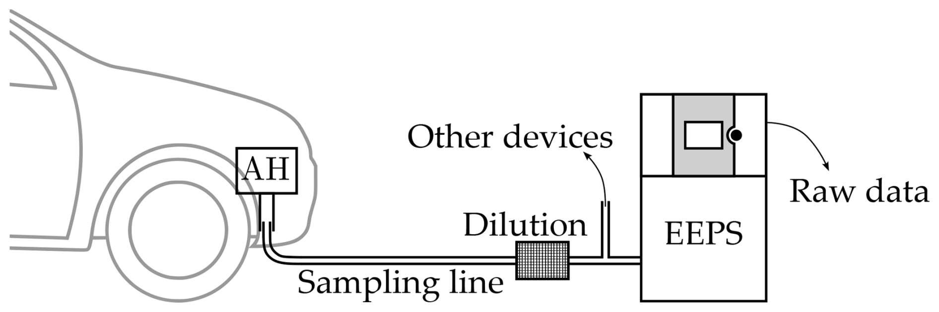
The PSD measurements in Oikarinen et al. (2022) were carried out using the Engine Exhaust Particle Sizer™ (EEPS) model 3090, manufactured by TSI Inc. The EEPS is a spectrometer that estimates PSD based on measurements of electrical mobility. A simplified schematic of the measurement setup in Oikarinen et al. (2022) is shown in Fig. 3, where exhaust gas from the AH is led to the EEPS through a sampling line with a length of 3.2 m and an inner diameter of 5 mm. Flow velocity through the line was 3.5 m s⁻¹, leading to a residence time of approximately 0.9 s. The sampling line was heated to 250 °C, and just before the EEPS the sample was diluted at a ratio that varied between 40:1 and 100:1 to allow for measurements of PN concentrations higher than the upper limit of the instrument.

Figure 3 A schematic of the measurement setup.

The operating principle of the EEPS is, in short, the following (TSI, 2015): a flow of exhaust gas is directed at the inlet, where particles in the gas are positively charged. The charged particles are then directed in a laminar flow through a cylindrical tube that has a positive high-voltage electrode column in the center and a stack of 22 circular electrometers on the outer wall. The electric field between the center electrode and electrometers deflects the particles outwards so that particles with high electrical mobility hit the electrometers near the inlet and particles with low electrical mobility hit the electrometers further along the stack. The striking particles generate currents that are proportional to the particle concentration. Measurements of these currents with their location along the stack can be inverted to give an estimate of the PN concentration. The operating size range of the EEPS is between 5.6 and 560 nm, and the whole size range is measured simultaneously, every 1 s in the present case.

An observation model (cf. Eq. 32) for the EEPS in terms of the raw electrometer currents can be written as (Wang et al., 2016a):

$$\begin{array}{}\text{(40)}& {\displaystyle }{\displaystyle }\mathit{y}=\mathbf{H}\mathit{f}+\mathit{e},\end{array}$$

where y∈ℝ²² is the measured current, f∈ℝ¹⁷ denotes a representation of the size distribution used by the EEPS, and e∈ℝ²² is measurement noise. The size distribution f is mapped to currents with an instrument matrix¹ $\mathbf{H}\in {\mathbb{R}}^{\mathrm{22}\times \mathrm{17}}$, which can be exported from the EEPS². Here we use the SOOT instrument matrix (Wang et al., 2016b), which TSI has developed to give more accurate estimates with soot particles than the instrument's default instrument matrix. To connect the aerosol bin model Eq. (3) to the observation model above, we map the size bin representation to f with an interpolation matrix $\mathbf{B}\in {\mathbb{R}}^{\mathrm{17}\times n_{\mathrm{B}}}$:

$$\begin{array}{}\text{(41)}& {\displaystyle }{\displaystyle }\mathit{f}=\mathbf{B}\widehat{\mathit{N}},\end{array}$$

where $\widehat{\mathit{N}}$ is a size bin representation of the PSD of the sample when it enters the EEPS after it has been altered by the sampling line. Finally, let Ξ represent the coagulation and wall diffusion model so that $\widehat{\mathit{N}}=\mathrm{\Xi }\left(\mathit{N}\right)$, and let ϕ denote a transformation from the log space to the absolute scale $\mathit{N}=\mathit{\varphi }\left(\stackrel{\mathrm{̃}}{\mathit{N}}\right)$. The full observation model is then $\mathit{y}=h\left(\stackrel{\mathrm{̃}}{\mathit{N}}\right)+\mathit{e}$, where the forward model is

$$\begin{array}{}\text{(42)}& {\displaystyle }{\displaystyle }h\left(\stackrel{\mathrm{̃}}{\mathit{N}}\right):=\mathbf{HB}\mathrm{\Xi }\left(\mathit{\varphi }\right(\stackrel{\mathrm{̃}}{\mathit{N}}\left)\right).\end{array}$$

To specify the covariance of the measurement noise, Γ_e, we assume that noise in each electrometer is independent of the other electrometers so that Γ_e is diagonal and consists of the noise variances ${\mathit{\sigma }}_{\mathrm{e},i}^{\mathrm{2}}$ of each electrometer i. These variances can generally be estimated from a calibration measurement with a minimal number of particles using a filtered sample. However, an analysis of the measurement data shows in this case that the noise seems to be approximately proportional to the measured current. Specifically, during time windows that are short enough, where the PSD is expected to stay constant and thus variation in the measured signal can be attributed to noise, the standard deviation of the measurements is roughly 5 %–15 % of the amplitude of the measurement. An exception to this is when the current drops below the electrometer noise floor. We therefore model the noise variance as

$$\begin{array}{}\text{(43)}& {\displaystyle }{\displaystyle }{\mathit{\sigma }}_{\mathrm{e},i}^{\mathrm{2}}=\text{max}\left({\mathit{\sigma }}_{\text{floor},i}^{\mathrm{2}},(\mathit{ϵ}{y}_i{)}^{\mathrm{2}}\right),i=\mathrm{1},\mathrm{\dots },\mathrm{22},\end{array}$$

where ${\mathit{\sigma }}_{\text{floor},i}^{\mathrm{2}}$ and y_i denote the noise floor and measured current of electrometer i, respectively, and ϵ denotes the noise level. Note that in the derivation of the likelihood we assumed that the noise and the unknowns are independent, but here some dependency is introduced between them. In practice, we thus use the measured values of y_i to assess the variance in Eq. (43) instead of reformulating the likelihood model to accommodate for a non-additive noise model that would result from the dependency between N and noise. The effect of this approximation, however, is minor if the noise level is not very high.

4.2 Inversions with simulated data

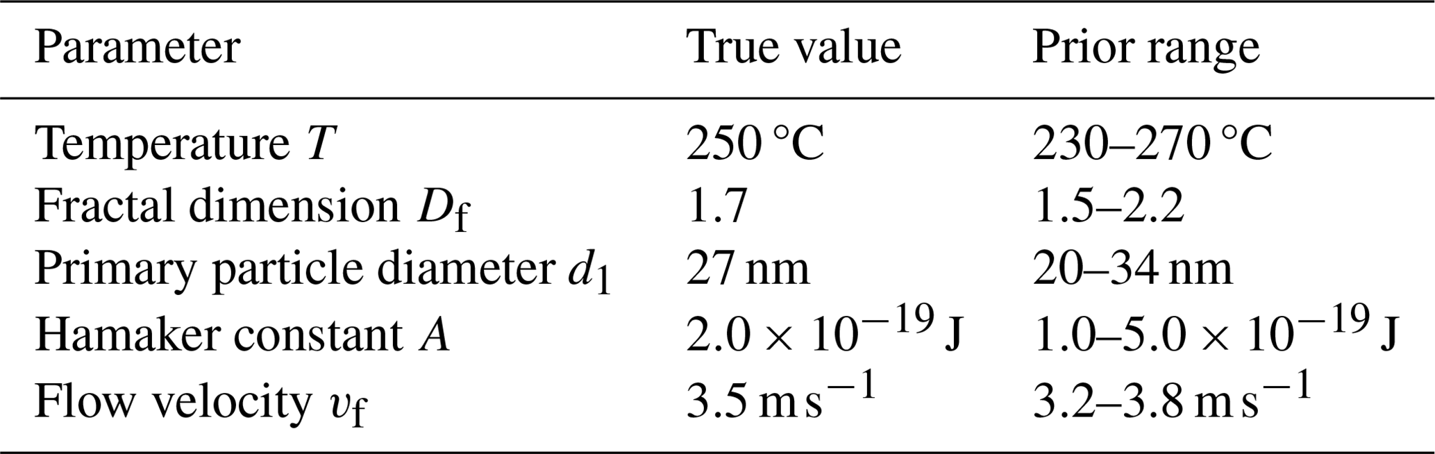
We created simulated data with the above model (Eq. 42), specifying the initial PSD and auxiliary parameters and adding noise with level ϵ=0.10. The initial number concentration was chosen to be high enough to clearly show coagulation effects but still realistic to be comparable to the number concentrations seen in the real measurements shown later. With simulated data, one must be careful to not commit a so-called inverse crime of using the same exact model to create the data and solve the inverse problem (Kaipio and Somersalo, 2006), which might lead to unrealistically good results. To ensure that the (tiny) numerical errors that arise due to discretizing the model are not the same, the data were created using a higher number of size bins than what was used in the inversion. We used 30 and 16 bins per decade for the data-generating and inversion models, respectively. The dilution ratio was set to 100:1, and the auxiliary parameters were set to the values given in Table 1. The expected value of the prior was set to ${\stackrel{\mathrm{̃}}{\mathit{N}}}_{*}=\log ({\mathrm{10}}^{\mathrm{3}}/w_{\text{bin}})$, where w_bin is the logarithmic bin width, and correlation length and variance were set to $\stackrel{\mathrm{̃}}{l}=\mathrm{12}/\mathrm{16}$ and $\stackrel{\mathrm{̃}}{a}=\mathrm{4}$, respectively.

Table 1 True values for the auxiliary parameters that were used to simulate synthetic data and the range over which they are allowed to vary when marginalizing.

4.2.1 Known auxiliary parameters

First, we carried out inversion with the same auxiliary parameters that were used to create the data. In this case, the only source of modeling error with respect to the accurate model used for generating the synthetic data is that caused by the coarser discretization of the particle size. The specified initial PSD and the corresponding generated noisy data points are shown in Fig. 4.

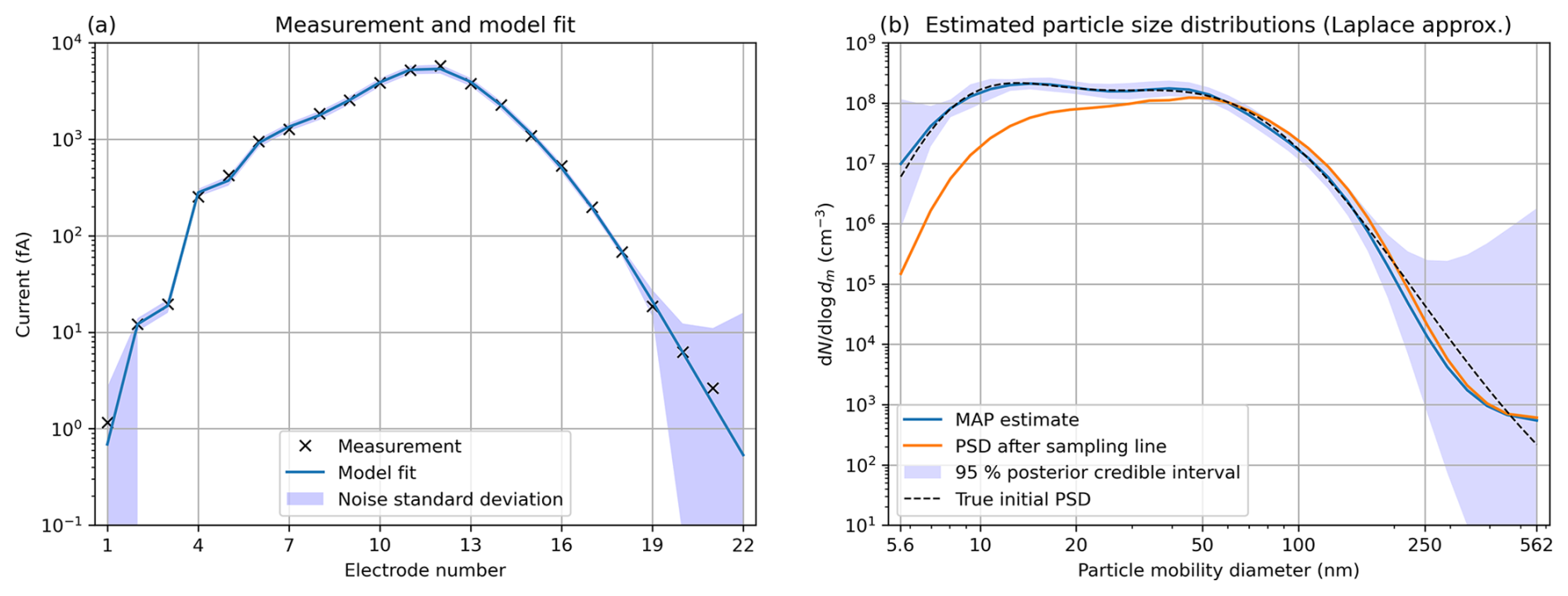
Figure 4 Synthetic data. (a) Simulated noisy data, model fit corresponding to the MAP estimate, and standard deviation of the measurement noise. (b) MAP estimate and 95 % posterior credible interval of the initial PSD, the MAP estimate propagated through the sampling line, and the true initial PSD.

The Gauss–Newton algorithm to compute the Laplace approximation for the initial PSD converged in nine iterations and took 0.4 s. All calculations in this paper were done on a laptop with an Intel(R) Core(TM) i7-12700H processor, using only a single CPU core. The Laplace approximation for the initial PSD and the PSD after the sampling line are also shown in Fig. 4. The PSD after the sampling line is calculated from the MAP estimate with the coagulation and wall diffusion model, and it depicts what would be estimated based on the EEPS data if the effects of the PSD evolution within the sampling line were neglected. A comparison between the estimated PSDs before and after the sampling line reveals a clear coagulation effect; the concentration of the smallest particles has reduced by up to 2 orders of magnitude, and these particles show up as a slightly higher number concentration of larger particles. The initial PSD can be said to be estimated well because the true initial PSD is found within the 95 % CIs over the whole size range. The relative error between the MAP estimate and the true initial PSD is 6.2 %.

To compute the true posterior, we ran the MCMC sampler for 200 000 iterations, which took 20 min. The first 25 % of the samples were removed as burn-in, and the remaining 150 000 samples had an average integrated autocorrelation time of 20.2 samples, which means there were over 7400 independent posterior samples in the chain. Figure 5a–c show the first variable of the MCMC chain (i.e., the smallest size bin) as an example, and a visual inspection of this and the rest of the chains showed no sign of convergence issues. In the remainder of this paper, it is assumed that a similar amount of sampling and a similar convergence analysis are done to validate each presented MCMC result. Figure 5d shows the CM estimate and 95 % CIs. Again, the initial PSD is estimated well and is found within the CIs. The relative error between the CM estimate and the true initial PSD is 7.1 %. The main differences compared to the Laplace approximation are that for particles larger than 200 nm, the CM estimate gives lower concentrations than the MAP estimate and that the CIs obtained by sampling are narrower than those of the Laplace approximation.

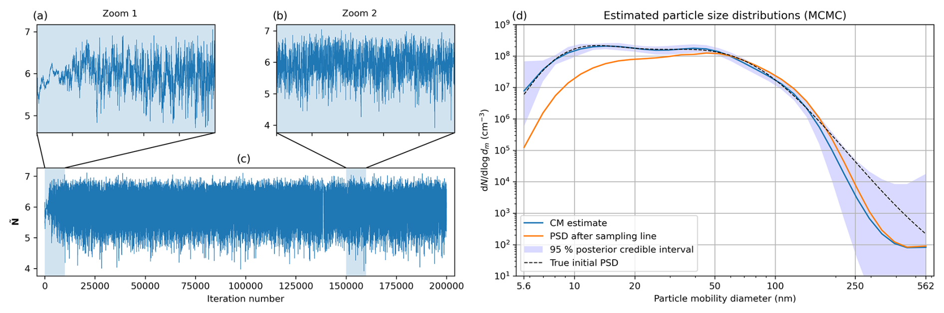
Figure 5 Synthetic data. The full MCMC chain, shown in (c), of the log number concentration of the first size bin and two zoomed-in sections showing (a) the beginning of the chain which is still in burn-in and (b) part of the chain when it has reached the steady state. (d) CM estimate and posterior credible intervals calculated with MCMC using the true auxiliary parameters.

4.2.2 Unknown auxiliary parameters

As mentioned in Sect. 3.4, it not always realistic to assume the auxiliary parameters are known accurately, and one approach to take their uncertainty into account is to model the auxiliary parameters as additional unknowns. An example of what can happen when just one parameter, here the fractal dimension, is incorrectly specified and its uncertainty not modeled is shown in Fig. 6. Here the data were generated with D_f=1.7, but in the inversion we used D_f=2.1, which is well within the possible values for the fractal dimension of soot. Figure 6a shows that, although not a dramatic change from the results in Fig. 5, the initial PSD is underestimated and the 95 % credible intervals do not always contain the truth, especially around 10 nm. In addition, the relative error between the CM estimate and the truth has increased to 18.8 %.

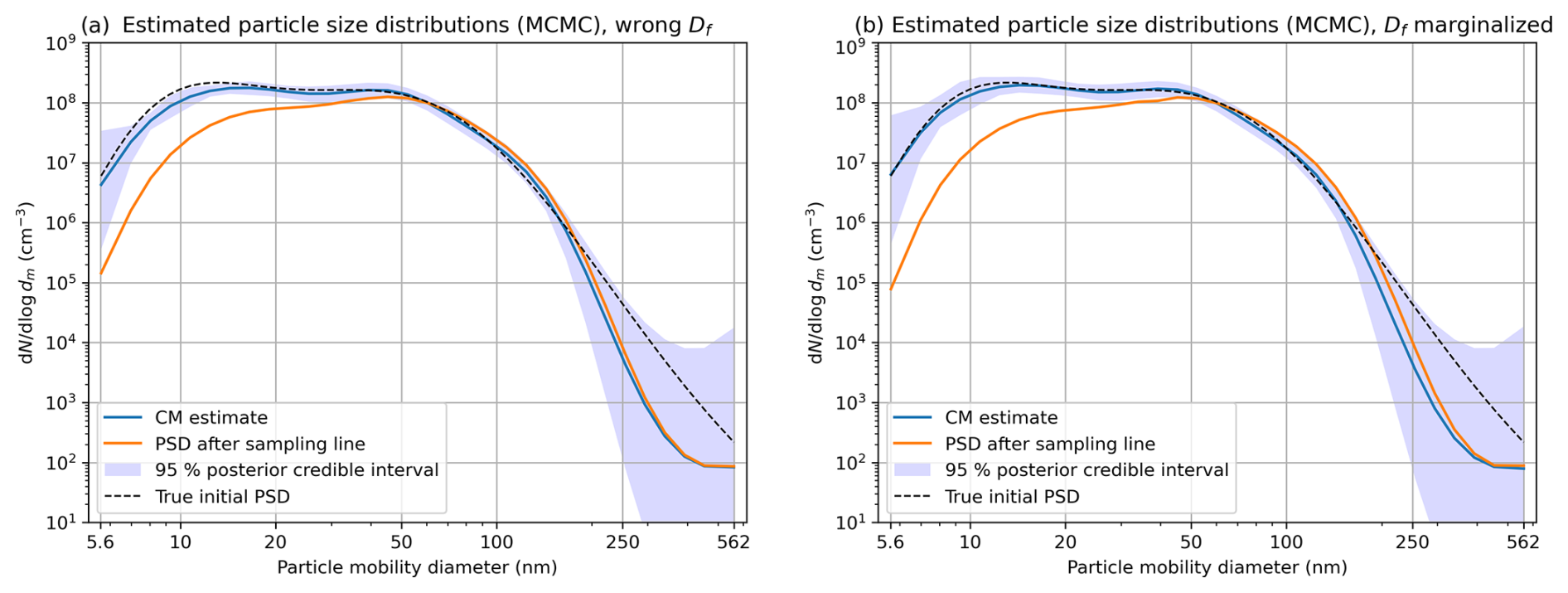
Figure 6 Synthetic data. (a) Posterior distribution with fractal dimension set to an incorrect value. (b) Posterior distribution with fractal dimension marginalized.

Let us now model D_f as an unknown and marginalize it. The resulting posterior is shown in Fig. 6b. Compared to the model where D_f was assumed to be accurate, the CIs of especially particles under 50 nm (which seem to be the most affected by coagulation) are considerably wider and now do include the true initial PSD. The CM estimate is also closer to the truth, with the relative error being 10.1 %.

Finally, let us marginalize all other auxiliary parameters as well, one by one and also all together. A complete list of the auxiliary parameters is given in Table 1, which also lists the ranges over which the integration is carried out. The fixed auxiliary parameters are held at their true values, except for D_f, which is set to 2.1. Figure 7a shows the full posterior in the case where all auxiliary parameters were integrated out at the same time. As is expected, the CIs in this case are wider than when only the fractal dimension has been marginalized. The relative error between the CM estimate and the truth is 6.8 %, which is even lower than when using the correct auxiliary parameters (7.1 %). However, this is likely just a coincidence related to, e.g., the chosen parameter ranges for marginalization and not something to be expected in general.

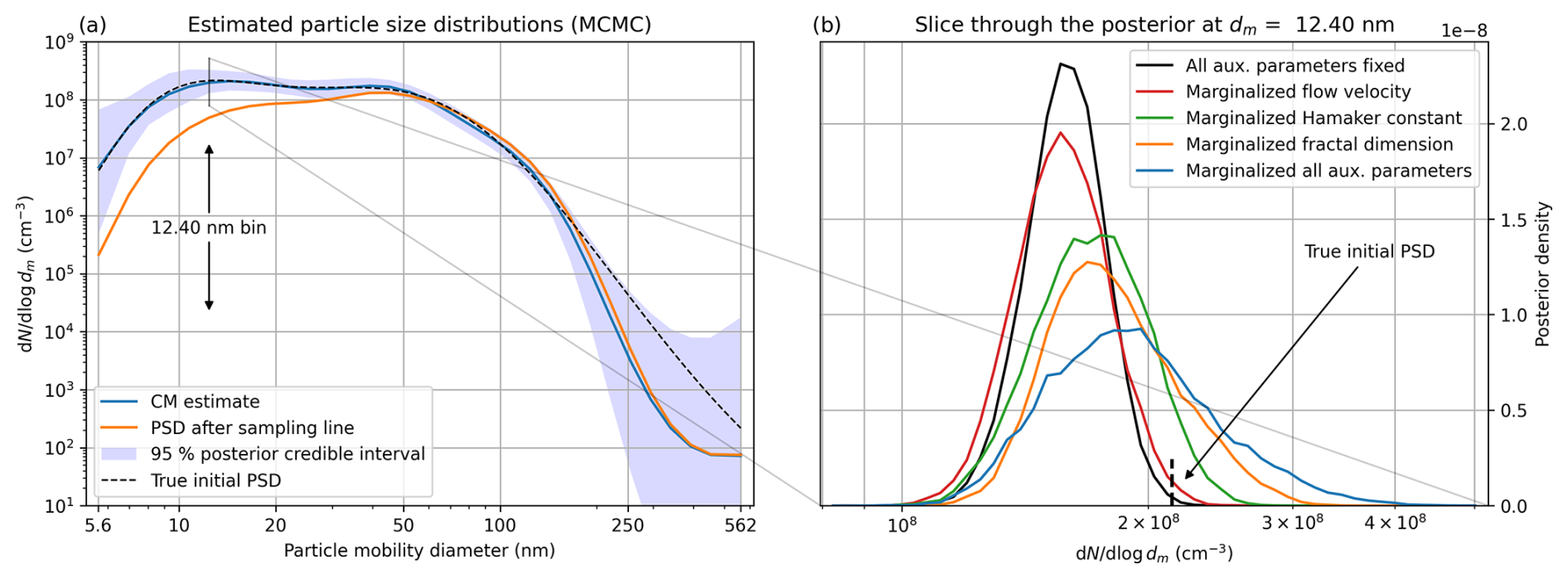
Figure 7 Synthetic data. (a) Posterior with all auxiliary model parameters marginalized. (b) Marginal posteriors of size bin number 5 (12.40 nm) with different auxiliary parameters marginalized.

To visualize the effects of uncertainties in different auxiliary parameters, let us focus on the posterior of a single size bin, i.e., a marginal posterior, which can be plotted as a histogram. Figure 7b shows these marginal posteriors at the sixth size bin (corresponding to d_m=12.40 nm) of five cases, where either the flow velocity, Hamaker constant, fractal dimension, all of the auxiliary parameters, or none of the auxiliary parameters has been marginalized. Note that the particle number in Fig. 7b is shown on the x axis, and the y axis now denotes the posterior probability density. The marginalization of temperature and the primary particle diameter is not shown because their effect on the posterior was minimal. Over the considered integration ranges, the effects of fractal dimension and the Hamaker constant were larger than that of the flow velocity, but in each case the marginalization increased the width of the CIs. Marginalizing all auxiliary parameters at the same time had naturally the largest effect.

4.3 Fuel-operated auxiliary heater measurement

The measurement campaign by Oikarinen et al. (2022) was carried out in February 2021 in Finnish winter conditions (−19 to −7 °C) over several days and with multiple vehicles. For the scope of this paper, we chose a measurement of one of the vehicles, a gasoline-powered 2019 Volkswagen Golf, to analyze as an example. The vehicle had an original equipment manufacturer (OEM)-installed AH manufactured by Webasto Ltd. Emissions of the AH were measured over a half-hour period, which included a cold start and shutdown of the AH. The EEPS was set to measure at 1 s intervals, leading to a total of around 1900 measurements. A more detailed description of the setup and analysis of the EEPS-inverted data is found in the original paper.

As mentioned earlier, computing the Laplace approximation is much faster than doing MCMC sampling and was therefore used to invert the dataset. MCMC was carried out at a few selected measurement points, discussed later. Discretization of the inversion model was set to 16 bins per decade so that the output bins were the same as those of the EEPS. The prior parameters were also kept the same as in the synthetic data inversion. However, because the choice of prior is subjective to some degree, in Sect. 5 we will briefly discuss different choices for the prior parameters and their influence on the PSD estimates. Further, because the data exhibit temporal smoothness, we used the previous MAP estimate as an initial guess for computing the next one, which reduced the number of Gauss–Newton iterations required to minimize the cost function. Inverting the whole dataset took 2 min and 20 s.

The MAP estimates of the initial PSD for the duration of the whole measurement are shown in Fig. 8. The results are qualitatively similar to the ones obtained directly from the EEPS, discussed in Oikarinen et al. (2022), where after startup, the AH emissions are relatively stable, followed by a burst of sub-20 nm particles during shutdown. However, there is a large difference in the total PN. Compared to the (diffusion-corrected) EEPS estimates, the total PN is on average 50 %–100 % higher in the MAP estimates, varying over the measurement period with a peak 230 % higher during the AH shutdown. Because coagulation affects the particle population differently depending on the particle size, also the ratio of PN between the MAP and EEPS estimates depends on the particle size. This is visualized in Fig. 9, which shows the ratio of PNs in the MAP and EEPS estimates for a few ranges of particles sizes. The number of particles under 20 nm may be over 3 times higher with the sampling line modeled, whereas the number of particles over 100 nm is typically reduced by up to 50 %.

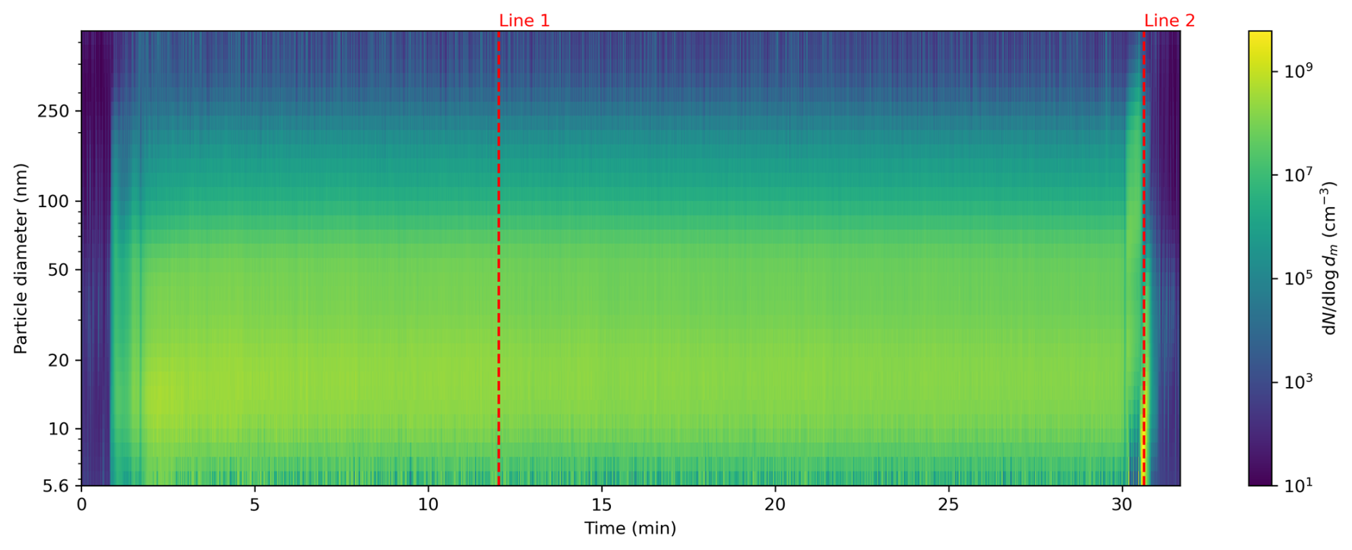
Figure 8 The MAP estimates for the initial PSD for a measurement of AH exhaust emissions of a 2019 Volkswagen Golf. Lines 1 and 2 denote measurement times analyzed in more detail.

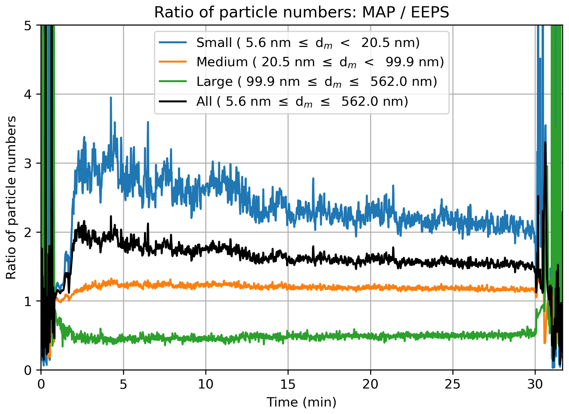
Figure 9 Ratio of PNs between the MAP and diffusion-corrected EEPS estimates during the example measurement. The MAP estimate of the number of small particles is 3 times that of the EEPS estimate in the beginning, whereas the number of particles over 100 nm is only around half of that of the EEPS estimate.

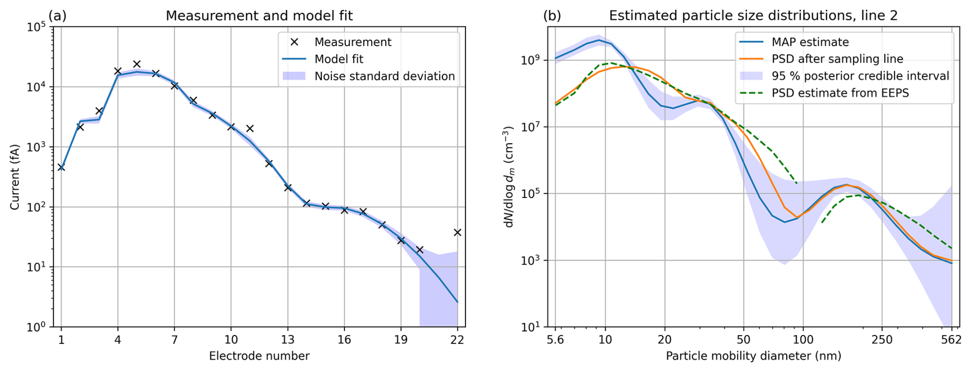
To compare the MAP estimates and EEPS output in more detail, let us analyze the two time instants shown as dashed red lines in Fig. 8. The time instant at Line 1 in the middle of the measurement corresponds to the steady state, and the time instant at Line 2 at the end is the time when the burst of sub-20 nm particles was at its peak. The Laplace approximations and the corresponding data fits at these points are shown in Figs. 10 and 11. First, in both examples, modeling the sampling line increases the number of the smallest particles in the estimates significantly while reducing the number of larger particles. Second, the PSDs after the sampling line are close to the PSD estimates from the EEPS, as they should be if our inversion algorithm was working correctly. The differences between them can be mostly attributed to the different inversion algorithms, choices of prior/regularization parameters, and handling of measurement noise. Inversion in the EEPS is based on a Tikhonov-regularized Gauss–Markov least-squares solution (Mirme et al., 2007; Mirme and Mirme, 2013; Wang et al., 2016a), but its details are not public. Moreover, the EEPS sometimes rounds the PSD estimates of some size bins down to zero, which can be seen in both Figs. 10 and 11 as gaps in the dotted line (values set to not a number (NaN) because of the log scale).

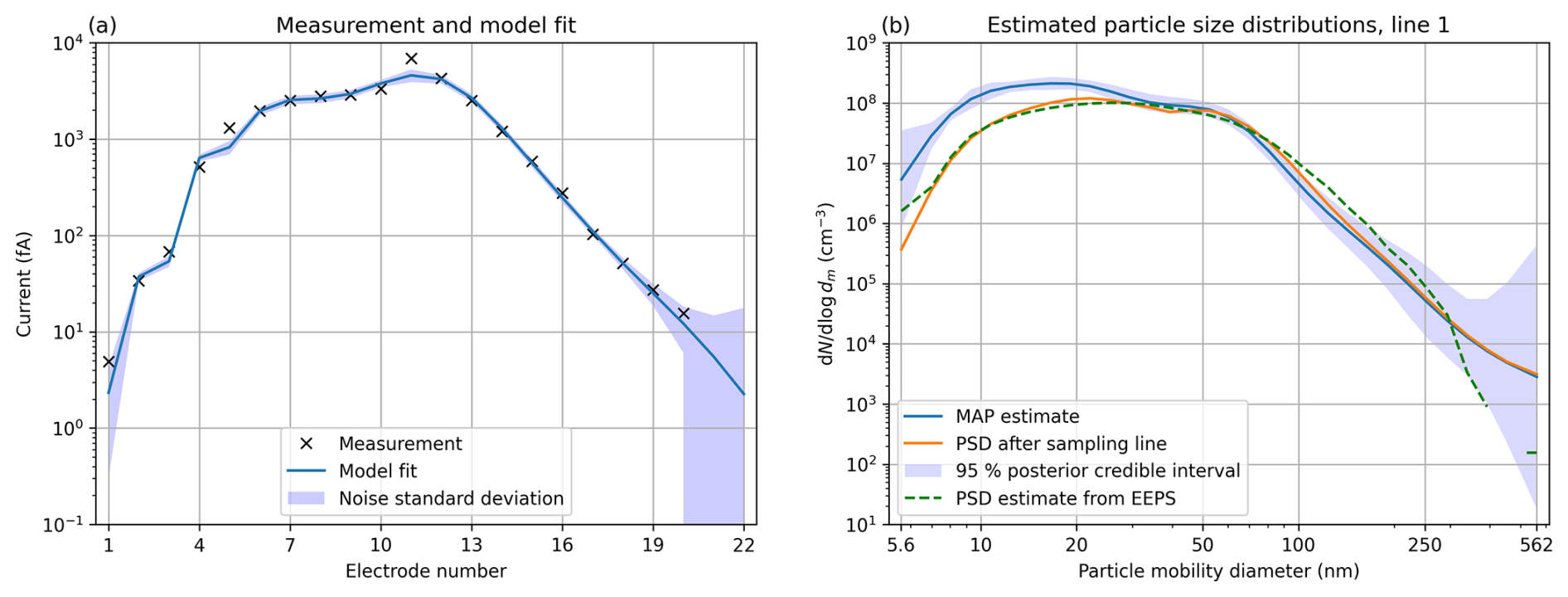
Figure 10 AH measurement at time instant 1 (Line 1 in Fig. 8). (a) Measured data, model fit corresponding to the MAP estimate, and standard deviation of the measurement noise. (b) MAP estimate and 95 % posterior credible interval of the initial PSD, the MAP estimate propagated through the sampling line, and the PSD estimate given by the EEPS.

Figure 11 AH measurement at time instant 2 (refer to the caption of Fig. 10).

Finally, we used MCMC to marginalize the auxiliary model parameters for the measurements at Line 1 and Line 2. The marginalization was carried out simultaneously for all five parameters over the ranges listed in Table 1. The results, shown in Fig. 12, resemble those of the synthetic tests in that the CM and MAP estimates are still close, but the 95 % CIs in the marginalized case are wider especially for the smallest particles.

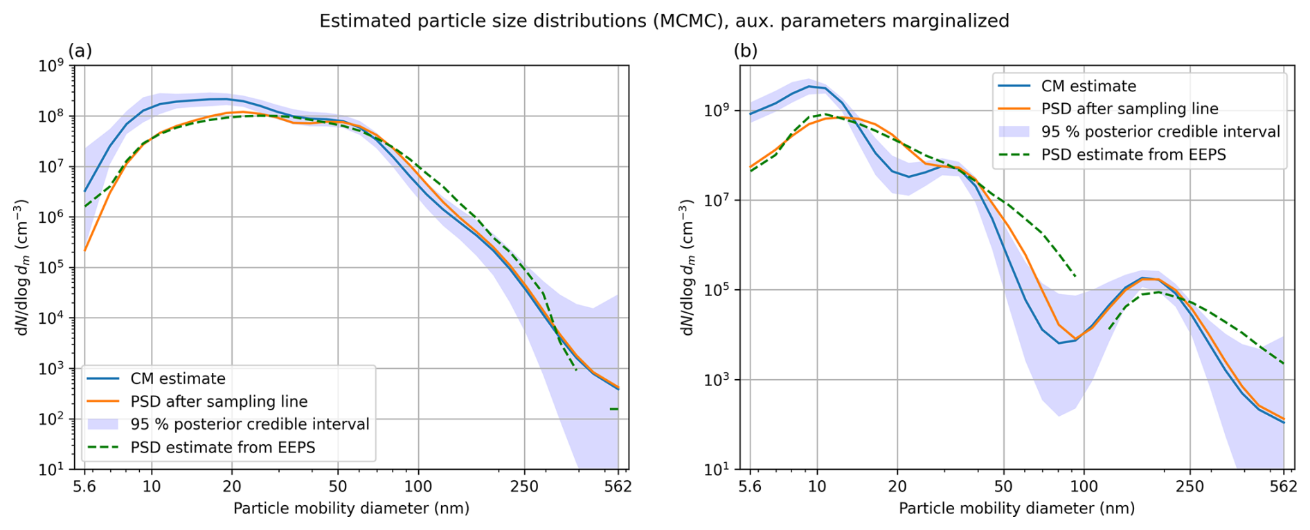
Figure 12 AH inversion results with all auxiliary parameters marginalized using MCMC for (a) Line 1 and (b) Line 2.

5 Discussion

The analyzed synthetic and real measurements show that sampling lines can have a major effect on the PSD when measuring the emissions of fuel-operated auxiliary heaters. The same observation obviously applies to any measurement where the sampling line is long and/or the PN concentration is high. When should one then be concerned about their measurements being distorted and consider applying, for example, the methods in this paper? The answer depends not just on the sampling line and PN concentration, but also on factors such as the particle shape, density, and fluid they are suspended in, which affect the coagulation rate and particle diffusion. In the context of the specific numerical example studied in this paper (see Fig. 4), our model shows that if the length of the sampling line was reduced from 3.2 m to, say, 1 m, the true initial total PN between 5.6 and 562 nm would still be about 33 % higher than what would be measured after the sampling line. It could be possible to define an indicator for a risk of distorted measurements based on the residence time and measured PN, but this is out of the scope of the present study.

A question regarding the inversion is if there is enough benefit to sampling the true posterior with MCMC compared to just computing the Laplace approximation. Based on the results in Sect. 4, the answer is in most cases no; the MAP and CM estimates are similar, and the Gaussian density seems to approximate the posterior well. Most importantly, computing the Laplace approximation is fast enough that it could even be combined with the inversion algorithm in the EEPS and still produce the estimates in real time, only now taking into account the effect of the sampling line and providing uncertainty estimates as well. A major benefit of running MCMC is that parameters in the forward model that we are uncertain of can be integrated out and their uncertainty propagated to the PSD estimates. The trade-off is an increased computation time. However, it could be possible to account for this uncertainty in an approximative manner while still retaining the speed of the Laplace approximation, using the Bayesian approximation error method (Kaipio and Somersalo, 2007; Kaipio and Kolehmainen, 2013), but this has not been pursued in this work.

As mentioned earlier, the inverse problem of estimating the PSD from measurements of currents is highly ill-posed even without considering the sampling line, and hence the uncertainty of the posterior depends to a large extent on the prior assumptions. For example, as the correlation length $\stackrel{\mathrm{̃}}{l}$ (see Sect. 3.1) is increased, the posterior will be constrained to more and more smooth solutions, which also constrains the posterior uncertainty. Let us demonstrate this in Fig. 13 by plotting the Laplace approximations of two posteriors which differ only in the prior correlation length. Note how in addition to smoothing out the MAP estimate, increasing the correlation length also decreases the width of the credible intervals, i.e., decreases the posterior uncertainty.

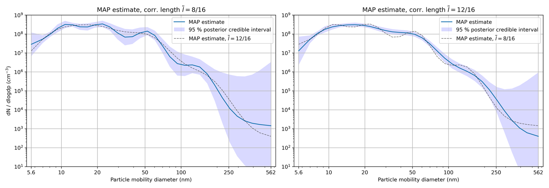
Figure 13 The influence of prior correlation length shown as MAP estimates and 95 % CIs with (a) $\stackrel{\mathrm{̃}}{l}=\mathrm{8}/\mathrm{16}$ and (b) $\stackrel{\mathrm{̃}}{l}=\mathrm{12}/\mathrm{16}$. The overlaid dotted lines are the MAP estimates from the neighboring figure for an easier comparison.

A source of uncertainty related to coagulation that has not been modeled in this work is the influence of particles larger and smaller than what we can measure, >562 and <5.6 nm, respectively, in the case of the EEPS. In the measurable range, coagulation with these larger particles results in higher-than-modeled particle losses, whereas coagulation with the smaller particles both introduces new particles at the lower measurable limit as well as causes particles in the measurable range to grow faster than modeled. Hence, the presence of particles larger than we can measure will lead to underestimating the initial PSD, and the presence of particles smaller than we can measure will have the opposite effect. According to a numerical simulation over a wide size range, however, if we assume the PSD outside the measurable range to continue the downward trend that is seen, for example, in Fig. 12a, its effect on the measured PSD is negligible.

Finally, there are a few loss mechanisms, including sampling losses (extraction of the aerosol at the sampling location), gravitational losses, inertial impaction, thermophoresis, and electrostatic deposition that may modify PN concentrations in a sampling line (Giechaskiel et al., 2012; Hinds, 1999). Most of these are, however, likely negligible in the case studied here and therefore not modeled. Sampling losses, gravitational losses, and inertial impaction mainly affect particles >1 µm, which is larger than what the EEPS can measure. On the other hand, inertial impaction can also cause losses of nanometer-size particles, but these are at or below the measured size range. Thermophoresis, the motion of particles in a temperature gradient, is potentially a major loss mechanism in sampling lines if there is a large temperature difference between the exhaust gas and the sampling line walls. In the measurement by Oikarinen et al. (2022), the sampling line was heated to 250 °C, which is very close to the temperature of the exhaust gas exiting the AH exhaust pipe, and hence the thermophoretic losses are expected to be minimal. Out of the mentioned loss mechanisms here, electrostatic deposition has the potential to have a major effect but at the same time is difficult to quantify because we do not know the charge on either the soot particles or the sampling line walls. We have hence ignored it in this paper but recognize that this effect may result in even higher particle losses than modeled so far.

6 Conclusions

In this article, we investigated how coagulation and wall diffusion in a sampling line modify a sample's particle size distribution and hence bias its measurement. Coagulation was found to become a significant factor especially at high PN concentrations because while the rate of wall diffusion is independent of the number concentration, the rate of coagulation is approximately proportional to its square. As an example of a high-PN case we studied the exhaust emissions of a fuel-burning road vehicle auxiliary heater, but it is worth noting that the presented method is applicable, and extendable, to any measurement where coagulation and/or any other aerosol process (such as condensation or evaporation) is suspected to affect the measurement. Through simulations and examining real data we found that, in a typical measurement setup, coagulation in the sampling line can reduce the total PN by more than 50 % and the number of small particles (<20 nm) even by an order of magnitude. The initial particle size distribution, not yet biased by the sampling line, can, however, be estimated from measurements that were done after the sampling line, given that we have a model for the processes in the sampling line.

Estimating the initial particle size distribution is an ill-posed inverse problem which we solved using methods in the Bayesian framework for inverse problems. In this framework, we can incorporate prior information about the size distribution and carry out a systematic calculation of the uncertainty related to the estimates. Two approaches to exploring the posterior probability density were tested: one where the posterior is fully characterized by MCMC sampling and another where the posterior is approximated as a Gaussian distribution. These resulted in similar estimates for the initial PSD, but both approaches also had distinct advantages. With the Gaussian approximation the inverse problem could be solved in a computationally efficient manner so that computing the estimates of the initial size distribution and its uncertainty could be done in real time even with measurement devices that have fast response times (1–10 Hz, for example). Using MCMC, on the other hand, we were able to take into account the (possible) uncertainty in the parameters of the coagulation and diffusion models, such as particle shape, using marginalization. This results in uncertainty estimates that are more consistent with what we assume to know about the problem but are computationally more demanding to calculate.

In conclusion, when the number concentration is high and the particles are small, the effect of coagulation in sampling lines should be taken into account when carrying out PSD or PN measurements. Otherwise, the particle numbers may be severely underestimated. Further, estimates of the PSDs have major uncertainties associated with them that traditional, deterministic inversion methods do not convey. Bayesian methods for uncertainty quantification could therefore prove useful in assessing the health and environmental impacts of fine particles in the future.