A gradient-boosted tree framework to model the ice thickness of the world's glaciers (IceBoost v1.1)

Knowledge of glacier ice volumes is crucial for constraining future sea level potential, evaluating freshwater resources, and assessing impacts on societies, from regional to global. Motivated by the disparity in existing ice volume estimates, we present IceBoost, a global machine learning framework trained to predict ice thickness at arbitrary coordinates, thereby enabling the generation of spatially distributed thickness maps for individual glaciers. IceBoost is an ensemble of two gradient-boosted trees trained with 3.7 million globally available ice thickness measurements and an array of 39 numerical features. The model error is similar to those of existing models outside polar regions and is up to 30 %–40 % lower at high latitudes. Providing supervision by exposing the model to available glacier thickness measurements reduces the error by a factor of up to 2 to 3. A feature-ranking analysis reveals that geodetic data are the most informative variables, while ice velocity can improve the model performance by 6 % at high latitudes. A major feature of IceBoost is a capability to generalize outside the training domain, i.e. producing meaningful ice thickness maps in all regions of the world, including on the ice sheet peripheries.

1 Introduction

Under atmospheric heating by human forcing, with few exceptions, glaciers have been retreating worldwide at unprecedented rates (Hugonnet et al., 2021), with projections predicting one-third of the mass loss at the end of the century in the most optimal +1.5 °C scenario (Rounce et al., 2023). At present, glacier melting contributes to sea level rise equally to ice sheets (Zemp et al., 2019; Fox-Kemper et al., 2021), with far-reaching implications for coastal communities worldwide (Pörtner et al., 2019). Ice mass loss from glacier shrinkage also impacts water availability for an estimated population of 1.9 billion people living in or depending on glacier-sourced freshwater (Huss and Hock, 2018; Rodell et al., 2018; Immerzeel et al., 2020).

Accurate and continuous knowledge of glacier ice thickness spatial distributions over time is thus of critical importance for informing and refining numerical models to better simulate future scenarios in a fast-changing climate (Zekollari et al., 2022). Measurement campaigns and surveys have led to direct ice thickness measurements for about 3000 of the more than 216 000 existing glaciers (Welty et al., 2020). The data are unsurprisingly sparse, but radar surveys from airborne campaigns have significantly increased the amount of measurements and coverage, particularly over polar regions. Knowledge of absolute glacier volume thus heavily relies on models or physical and mathematical interpolations.

An array of models has been proposed over time, with varying degrees of applicability (Farinotti et al., 2017). Only two have been applied to all glaciers on Earth. They are based on principles of ice flow dynamics and use surface characteristics, including ice surface velocity. The mass conservation approach by Huss and Farinotti (2012) has been extended with four additional regional models to produce a global consensus ensemble (Farinotti et al., 2019). More recently, Millan et al. (2022) also provided a global solution, leveraging a complete coverage of glacier velocities and using a shallow ice approximation (Cuffey and Paterson, 2010) with basal sliding. The degree of applicability of thickness inversion methods is broad. The main challenges relate to the validity of the underlying physical assumptions, parameter calibration, and availability and quality of model input data. As an example, the shallow ice approximation simplifies the stress field by neglecting longitudinal stresses, lateral drag, and vertical stress gradients. This setup works well in the interior of an ice sheet or with ice masses with small depth-to-width ratios. On mountain glaciers, Le Meur et al. (2004) found that this approach can be acceptable for slope values less than 20 %. In relation to challenges of parameter calibration, Millan et al. (2022) tuned the creep parameter A on a regional basis using ice thickness measurements, if present, and, if not, from other regionally averaged values. The basal sliding was parameterized indirectly by imposing assumptions of surface ice velocity : slope ratios. Input data are crucial – for example, a shallow ice approximation can only by used if the ice velocity product is available. For glaciers not covered by these data, the method cannot be applied. Previous methods have also suffered from incomplete surface ice velocity, which is now becoming globally available, and quality surface mass balance data. We refer the reader to Farinotti et al. (2017) for a comprehensive overview of thickness inversion models, their advantages, and their limitations.

A parallel line of research is exploring machine learning methods. Few approaches based solely on deep learning have been explored so far. Clarke et al. (2009) proposed a multi-layer perceptron trained on neighbouring deglaciated regions to reconstruct glacier bedrocks. This method does not invoke physics but assumes similarity between glacier bedrocks and the topography of nearby ice-free landscapes. Convolutional neural networks (CNNs) are now the state-of-the-art architectures for physical model emulators, and they have gained traction in glaciology with Jouvet et al. (2022) and Jouvet (2023). Trained to represent physical models with a much cheaper computational cost, emulators have the versatility to both compute forward modelling and invert for ice thickness. Uroz et al. (2024) trained a CNN to produce ice thickness maps on 1400 Swiss glaciers by ingesting surface velocity and digital elevation model (DEM) maps, with their ground truth consisting of ice thickness fields obtained by a combination of experimental data and glaciological modelling. Growing attention is being directed to physics-informed neural networks, as they provide a natural setup for generating an approximate solution of a differential equation and minimizing the misfit with observational data, if any. For a review, we refer the reader to Liu et al. (2024).

In this work, we present IceBoost, a machine learning system designed for modelling ice thickness across all of Earth's glaciers, including continental glaciers, ice caps, and ice masses at the edges of ice sheets. The method is not explicitly based on any physical law. It is fully data-driven yet contains the versatility to incorporate many relevant features that do not easily lend themselves to classical physics modelling. The only theoretical consideration of significance relates to the architecture choice. We approach the problem as a machine learning regression task, predicting ice thickness at any arbitrary point within a glacier's boundary. IceBoost employs an ensemble of two gradient-boosted decision tree models, XGBoost (Chen and Guestrin, 2016) and CatBoost (Prokhorenkova et al., 2018), both trained with ice thickness as a target. The target data are naturally tabular-structured (measurements localized in space) and are extracted from the Global Ice Thickness Database (GlaThiDa, or GTD hereafter), a centralized effort by the World Glacier Monitoring Service (WGMS) detailed by Welty et al. (2020). The model is informed by a set of 39 numerical features, extracted from an array of (either gridded or tabular) products and organized in a tabular structure. While CNNs are best suited to operation on gridded products (images) when data are tabular-structured, tree-based models often provide a much faster and powerful alternative to neural networks, as highlighted from theoretical considerations (Grinsztajn et al., 2022) and empirically from machine learning practitioners. CNNs are also typically very demanding in terms of training data and computational power and require elaborate methods for the interpretability of internal layers. Instead, gradient-boosted systems allow for straightforward interpretability in terms of which features are important for the thickness inversion of individual glaciers using Shapley values (Lundberg and Lee, 2017).

In the following sections we introduce the model concepts (Sect. 2), describe feature interpretability (Sect. 3), illustrate the model inference and compare its performance against existing global solutions (Sect. 4), describe some limitations and possible improvements (Sect. 5), and consider the computational cost (Sect. 6) before we conclude (Sect. 7).

2 Methods

Hereafter, we describe the datasets used to generate the features for model training and inference. The mass balance feature is presented in Appendix A for brevity.

2.1 Datasets

As a ground truth, we use the GlaThiDa v.3.1.0 dataset (GlaThiDa Consortium, 2020; Welty et al., 2020), which comprises 3.8 million ice thickness measurements, integrated with an additional 11 000 measurements from 44 glaciers included in the IceBridge MCoRDS L2 Ice Thickness product (Paden et al., 2010). The model is trained using the glacier geometries digitized and stored in the Randolph Glacier Inventory (RGI) v.62 (Pfeffer et al., 2014). This version extends version 6 with 1000 additional ice bodies from the Greenland periphery (connectivity level 2 to the ice sheet), hereafter still referred to as glaciers. RGI v.62 thus provides the opportunity to train and test the model's ability to reproduce thickness patterns in an ice sheet flow domain, a region with an extensive amount of available thickness data from the IceBridge mission. RGI glacier geometries include both the glacier external boundaries and the ice-free regions contained therein (hereafter referred to as nunataks). At the inference time, IceBoost supports geometries from either RGI v.62 (n = 216 502) or RGI v.70 (n = 274 531).

Hugonnet et al. (2021)Hugonnet et al. (2021)Millan et al. (2022)Joughin et al. (2016)Mouginot et al. (2019)

Table 1 List of features and products used by IceBoost, together with their units, number of variables, and primary dataset for their calculation. Local features are flagged by circles. No circles indicate glacier mean values. RGI shapefiles are mostly derived from 30 m resolution satellite data, and therefore variables calculated from RGI are indicated with 30 m horizontal resolution. The Tandem-X EDEM has a 3 arcsec horizontal resolution, corresponding to approximately 30 m at the Equator. The model is trained with ice thickness data from the GlaThiDa Consortium (GlaThiDa Consortium, 2020). See Fig. 2 for an analysis of the predictive power of the features.

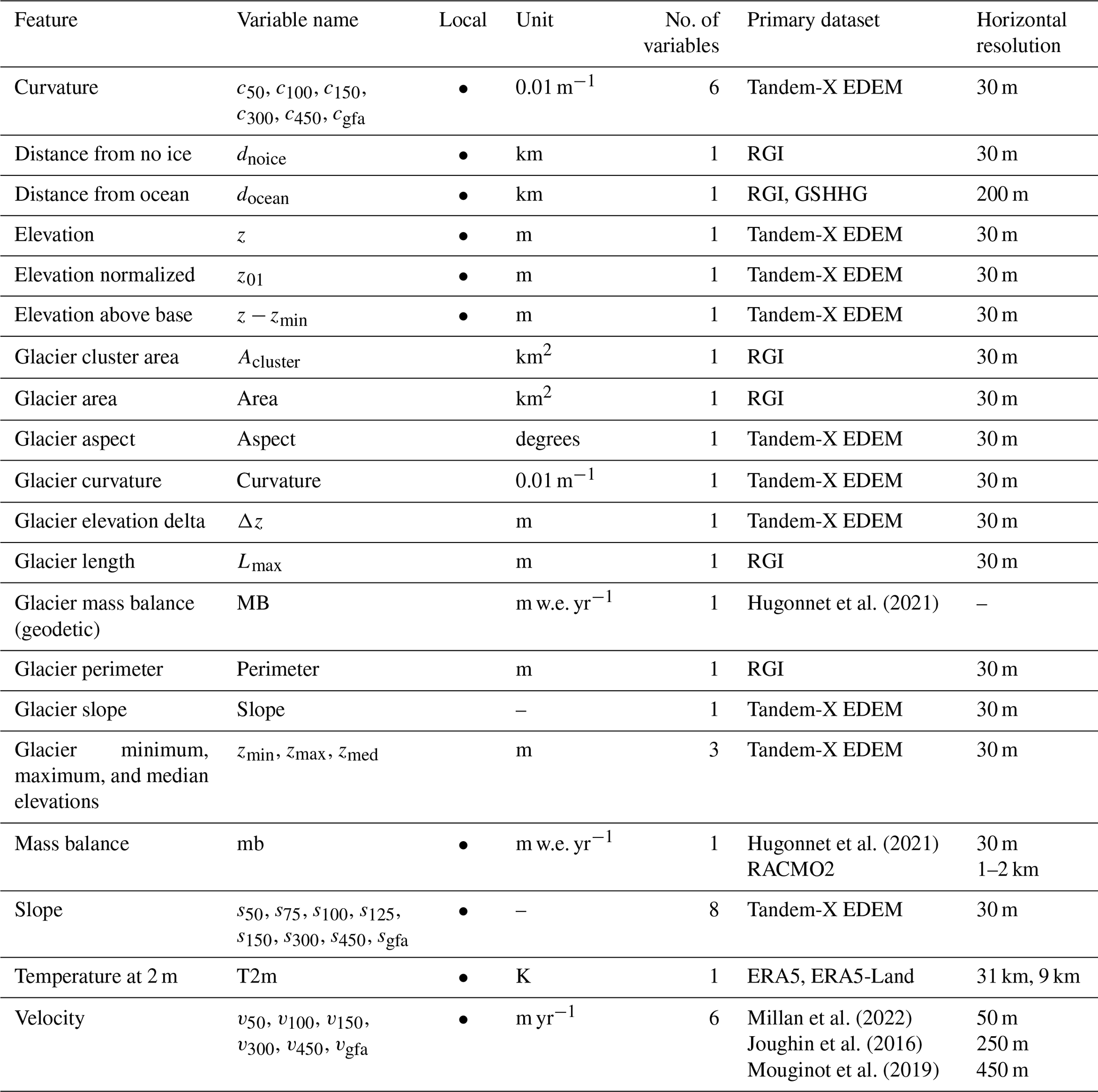
The features used to train the model are computed from various datasets presented hereafter (Table 1). Elevation and geodetic information is computed from the global Tandem-X 30 m Edited Digital Elevation Model (EDEM; Bueso-Bello et al., 2021; González et al., 2020; Martone et al., 2018). The modelled spatially distributed surface mass balance from Greenland and Antarctica is obtained from the Regional Atmospheric Climate Model (RACMO2) products available at different spatial resolutions (Noël et al., 2018; Noël and van Kampenhout, 2019; Noël et al., 2023). Glacier-integrated mass balance values are imported from Hugonnet et al. (2021). Temperature at 2 m (T2m​​​​​​​ hereafter) fields is taken from ERA5 and ERA5-Land (Hersbach et al., 2020; Muñoz Sabater et al., 2021). Surface ice velocity fields are taken from Millan et al. (2022), except for glaciers listed in Antarctica (RGI 19) and Greenland (RGI 5), where we use the velocity products from Mouginot et al. (2019) and Joughin et al. (2016), respectively.

Our solutions are compared with existing global models while acknowledging that additional solutions exist with regional validity. Outside the ice sheets, we compare them with the Farinotti et al. (2019) ensemble and with the shallow ice approximation by Millan et al. (2022). On the Antarctic periphery (RGI 19), we compare them with Farinotti et al. (2019) and BedMachine v3.7 (Morlighem, 2022). On the Greenland periphery, we compare them with Farinotti et al. (2019) and BedMachine v5 (Morlighem et al., 2022). BedMachine Greenland and Antarctica are complete modelled bed topographies and ice thickness maps of the two ice sheets. They are constructed using different methods in different regions and are continuously updated. Mass conservation is typically applied where knowledge of the surface speed is robust and sufficient. Elsewhere, other methods like kriging interpolation and streamline diffusion are adopted. At the time of writing, BedMachine Greenland v5 uses Millan et al. (2022) for isolated glaciers and ice caps and mass conservation or kriging interpolation elsewhere.

2.2 Training features

The model is trained with a set of 39 numerical features extracted from the above-mentioned datasets (Table 1). Some features are local, i.e. vary within the glacier. Others are per-glacier constants. We use the main variables of a steady-state mass-conservation-based inversion or physically based approximations (Huss and Farinotti, 2012; Millan et al., 2022): ice velocity, mass balance, and spatial first- and second-order gradients of the elevation field (hereafter referred to as slope and curvature, respectively). We extend the amount of information with geometrical features that relate to topographies (e.g. U-shaped valleys) crafted in alpine landscapes (distance to margins or internal deglaciated patches) and metrics of glacier size which are typical of scaling approaches (Bahr et al., 2015). We also use variables that carry a fingerprint of a thermal regime and a climate setting (temperature and distance from the ocean). It is worth mentioning that, in a gradient-boosted tree approach, the same variable can be used more than once in the decision tree scheme. For training, the features are calculated and stored offline in a training dataset. At the inference time, all features are calculated on the fly.

2.2.1 Constant features

The following features are per-glacier constants: area (Area), perimeter (Perimeter), glacier minimum (z_min), maximum (z_max) and median (z_med) elevations, glacier elevation delta ($\mathrm{\Delta }z=z_{max}-z_{min}$), length (L_max), and area of glacier cluster (A_cluster).

The elevations are calculated from the DEM. The areas, perimeter, and glacier length are calculated from the glacier geometries. The areas only include the iced region and exclude nunataks. The area of a glacier cluster is determined by summing the areas of all glaciers connected to the glacier under investigation, considering connections up to a maximum level of 3. This feature indicates whether a glacier is isolated (Area = A_cluster) or part of a larger system. The glacier length (L_max) is calculated as the maximum distance between any pair of points that lie on the glacier convex hull (Appendix A1). The glacier convex hull is referred to as the smallest convex set that contains the glacier itself. Except for the elevations, the other constant features are metrics of glacier size. Extensive previous research has been directed at empirical scaling laws to relate glacier volume to, for example, its area (Bahr et al., 2015). IceBoost retains the information carried by metrics of glacier size in a machine learning approach, without imposing explicit laws.

2.2.2 Distance from ice-free regions (d_noice) and distance from the ocean (d_ocean)

Given a point x₀ inside a glacier g, we calculate the distance to the closest ice-free pixel. Such a target point may lie within or outside the glacier. We define a glacier cluster as the collection of all neighbouring glaciers. For example, three glaciers $\mathit{\{}{g}_{\mathrm{1}},g_{\mathrm{2}},g_{\mathrm{3}}\mathit{\}}$ form a cluster if g₁ shares a pixel with g₂ and g₂ shares a pixel with g₃, despite g₁ and g₃ not necessarily being adjacent glaciers. The glacier cluster is calculated by detecting, starting from the glacier that contains the point x₀, all its proximal neighbours. The procedure is repeated iteratively for every neighbouring glacier until no further neighbours are found. In discrete mathematics, this structure is a graph. Once the cluster is computed, all internal shared borders (the ice divides) of the cluster are removed, while internal ice-free nunataks are kept. This procedure potentially results in collections of up to thousands of geometries per cluster. The calculations to create the cluster are made by setting up a graph-network structure using the NetworkX Python library (Hagberg et al., 2008).

The minimum distance from the point x₀ to an ice-free region (d_noice) is the minimum distance between x₀ and all points x lying on the cluster's valid geometries:

$$\begin{array}{}\text{(1)}& d_{\mathrm{noice}}\left({\mathit{x}}_{\mathrm{0}}\right)=\arg \underset{\mathit{x}\in \mathrm{cluster}}{min}d({\mathit{x}}_{\mathrm{0}},\mathit{x}).\end{array}$$

The valid geometries can either be the cluster's external boundaries or all of the cluster's nunataks. The distances are computed by querying K-dimensional trees, an approximate nearest-neighbour lookup method, on the geometries defined in the Universal Transverse Mercator (UTM) projection. We compare the proximal points obtained from this method with those from a brute-force calculation and find indiscernible results. The pipeline is computed as a feature for the creation of the training dataset and at inference time for every generated point. For computational speed-up, at inference time, the number of geometries K used by the KD tree can be capped to the closest 10 000 geometries. An example for d_noice is shown in Fig. A1.

Similar to the distance to ice-free regions, we calculate the closest distance to the ocean. We use the Global Self-consistent, Hierarchical, High-resolution Geography Database (GSHHG), containing all the world's shoreline geometries at resolution “f” (full). Like d_noice, d_ocean is calculated by querying a KD tree in the geometries in UTM projection. We find this feature to be relatively unimportant on continental glaciers far from the coasts but increasingly informative at high latitudes, where many marine-terminating glaciers are located.

2.3 Elevation, curvature, and slope

We use the DEM to calculate the following features: local elevation z, elevation above the glacier's lowest elevation $z-z_{min}$, elevation normalized between 0 and 1 $z_{\mathrm{01}}=(z-z_{min})/(z_{max}-z_{min})$, curvature, and slope.

To calculate the slopes, the DEM tiles are first projected in UTM and differentiated, and the resulting vector magnitude is convoluted using Gaussian filters of different kernel widths to capture the variability across different spatial scales: 50, 75, 100, 125, 150, 300, and 450 m and an adaptive filter, af, in Eq. (2):

$$\begin{array}{}\text{(2)}& \mathrm{af}={\displaystyle \frac{\mathrm{2}A}{\mathit{\pi }{L}_{max}}},\end{array}$$

where A and L_max are the area and glacier maximum length features. af corresponds to the semi-minor axis of an ellipse of area A and the semi-major axis $L_{max}/\mathrm{2}$. This kernel aims at estimating the glacier spatial size. For values lower than 100 or above 2000 m, af is capped to these values. Each training point yields eight slope features. The purpose of using many kernels is to allow the model the freedom to account for different glacier spatial scales. For small glaciers, the small kernels are found to be more important than the bigger kernels and vice versa (Fig. 2).

To limit the computational cost, for the calculation of the curvature, the elevation field is smoothed using only the 50, 100, 150, 300, and 450 m and af kernels, thus resulting in six features per point. All geodetic features are obtained from linear interpolation.

The model is also informed by glacier-integrated (i.e. mean) values of slope, curvature, and aspect (Slope, Curvature, and Aspect; Table 1).

2.3.1 Mass balance

Glacier thickness is controlled by ice flow and mass balance (Cuffey and Paterson, 2010). The latter is the net result of positive precipitation and mass loss mechanisms, both at the surface and at the glacier bed. We use two different mass balance features. The first is the glacier-mean 2000–2020 mass balance value imported as is from Hugonnet et al. (2021). Such a dataset is available for RGI v6 and is therefore suitable for training our model and for inference over RGI v6. For inference on the latest RGI v7 geometries, we reference the two RGI datasets or impute the regional mean for missing IDs. The second mass balance feature is a local map of mass balance, obtained by downscaling glacier-integrated values for non-polar glaciers or directly interpolating RACMO for ice sheet glaciers. It is discussed in Appendix A2 and Appendix D.

2.3.2 Surface ice velocity

Presently, the surface ice velocity is available with almost global coverage and is therefore used as an input feature. The velocity magnitude fields are smoothed with the six kernels 50, 100, 150, 300, and 450 m and af, and they are linearly interpolated. The velocity products used have different resolutions: Millan et al. (2022) (all regions except for Greenland and Antarctica), Joughin et al. (2016) (Greenland), and Mouginot et al. (2019) have resolutions of 50, 250, and 450 m, respectively. If the product resolution is higher than any kernel size, the kernels are set to match the product resolution. For every training point, a total of six velocity features are obtained. At the inference time, the missing velocity features are treated according to the imputation policy described in Appendix B2.

2.3.3 Temperature

The model is informed with the local T2m as a loose regional indicator of thermal regime and ice thickness. Although a weak indicator, this variable may still be useful in a decision tree, helping to split the data at earlier stages and enabling more powerful features to drive predictions at deeper levels of the tree structure. We also use this feature to provide regional context to a global model. We use ERA5-Land (0.1° grid spacing; Muñoz Sabater et al., 2021) and, for the missing pixels caused by imperfect fractional land masks along the coastlines and islands, we incorporate the ERA5 T2m field (0.25° resolution; Hersbach et al., 2020), bilinearly interpolated to the ERA5 0.1° resolution. We consider monthly maps over 2000–2010 and average them over this time period to generate one single global temperature field. This map is linearly interpolated at the measurement points (training) or at the generated points (inference time).

2.4 Data pre-processing and time tagging

A significant number of zero-thickness measurements are found in GlaThiDa. While some of these measurements are found close to glacier boundaries, at times they are found inside glacier geometries. We decided to discard all GlaThiDa zero-thickness entries. GlaThiDa thickness data from glacier RGI60-19.01406 (peripheral glacier in Antarctica; 65.5° S, 100.8° E; maximum elevation 500 m a.s.l.) are erroneously registered with a factor 10 too much (up to more than 3000 m of ice). We divide these data by 10. All datasets used in this work are tied to different time intervals. The glacier outlines refer to 2000–2010 for most glaciers (Pfeffer et al., 2014). The ice surface velocity outside the ice sheets is tied to 2017–2018 (Millan et al., 2022). The Tandem-X EDEM results from acquisitions between 2011 and 2015. The GlaThiDa dataset stores ice thickness measurements from 1936 to 2017. The ERA5 and ERA5-Land fields are tagged to 2000–2010. To homogenize temporally as much as possible all datasets in the creation of the training set while maximizing its size, all ice thickness measurements older than 2005 are discarded. In addition, we discard all measurements that lie outside glacier boundaries or inside nunataks. Overall, the model is conservatively estimated to be trained on data spanning from 2005 to 2017.

The resulting GlaThiDa dataset comprises 3.7 million points collected from 2300 glaciers (Fig. 1). To reduce the amount of correlated data that are close to each other and reduce computational costs, the training dataset is spatially downscaled. Each glacier is divided into a grid of 100 × 100 latitude–longitude pixels, and the per-pixel average is computed for all features and thickness data. The original dataset of 3.7 million points is thus encoded into a final training dataset of 300 000 entries. For baseline comparison, the thickness fields from Millan et al. (2022) and Farinotti et al. (2019) were also downscaled.

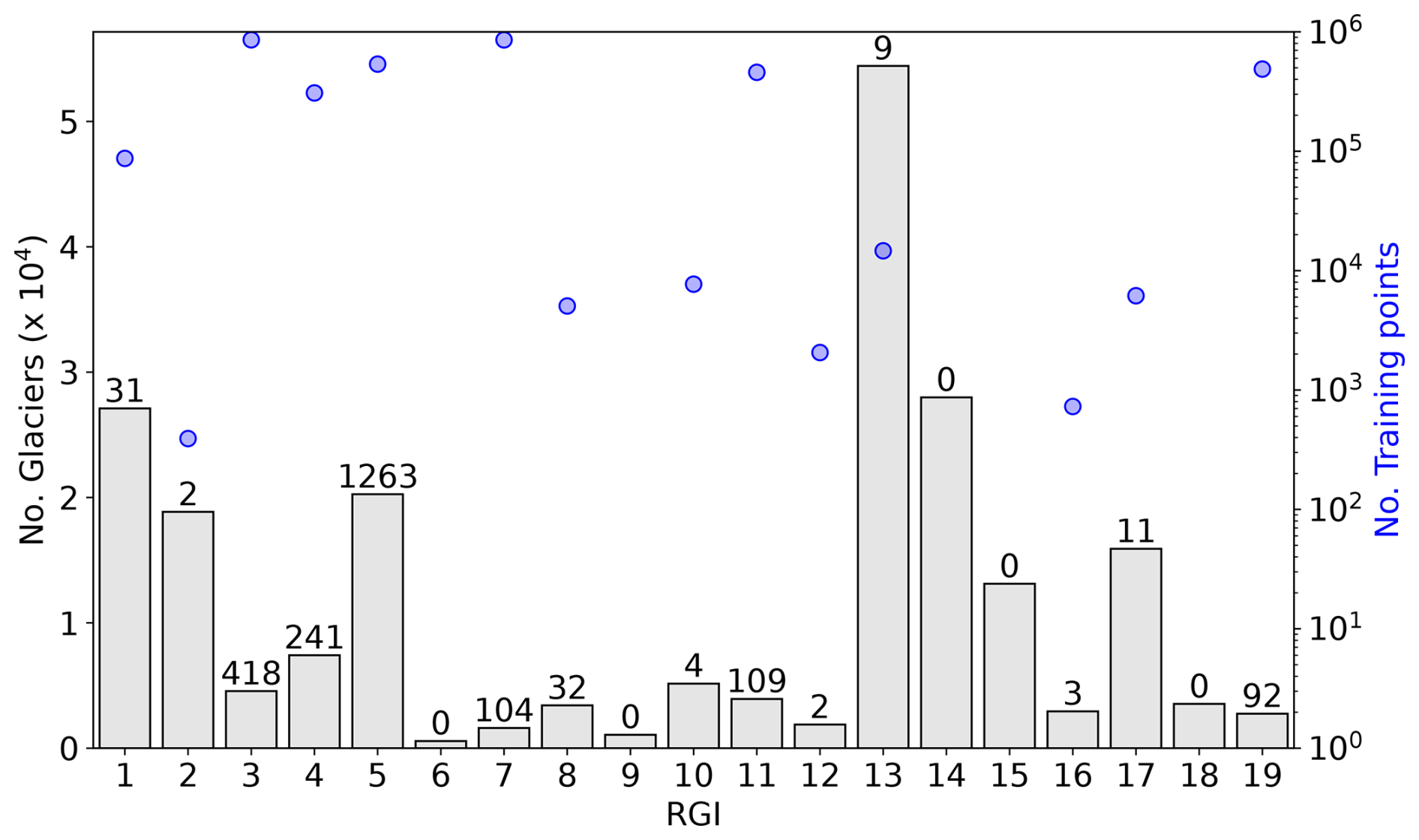
Figure 1 Statistics of glaciers and training data for each Randolph Glacier Inventory (RGI) region. The total number of glaciers in each region is represented by bar lengths on the left axis (10⁴). The numbers over each bar represent the absolute counts of glaciers with available training data (blue circles, right axis). Out of 216 000 glaciers worldwide, only 2300 contain at least one training point. RGI regions 6, 9, 14, 15, and 18 have no training data.

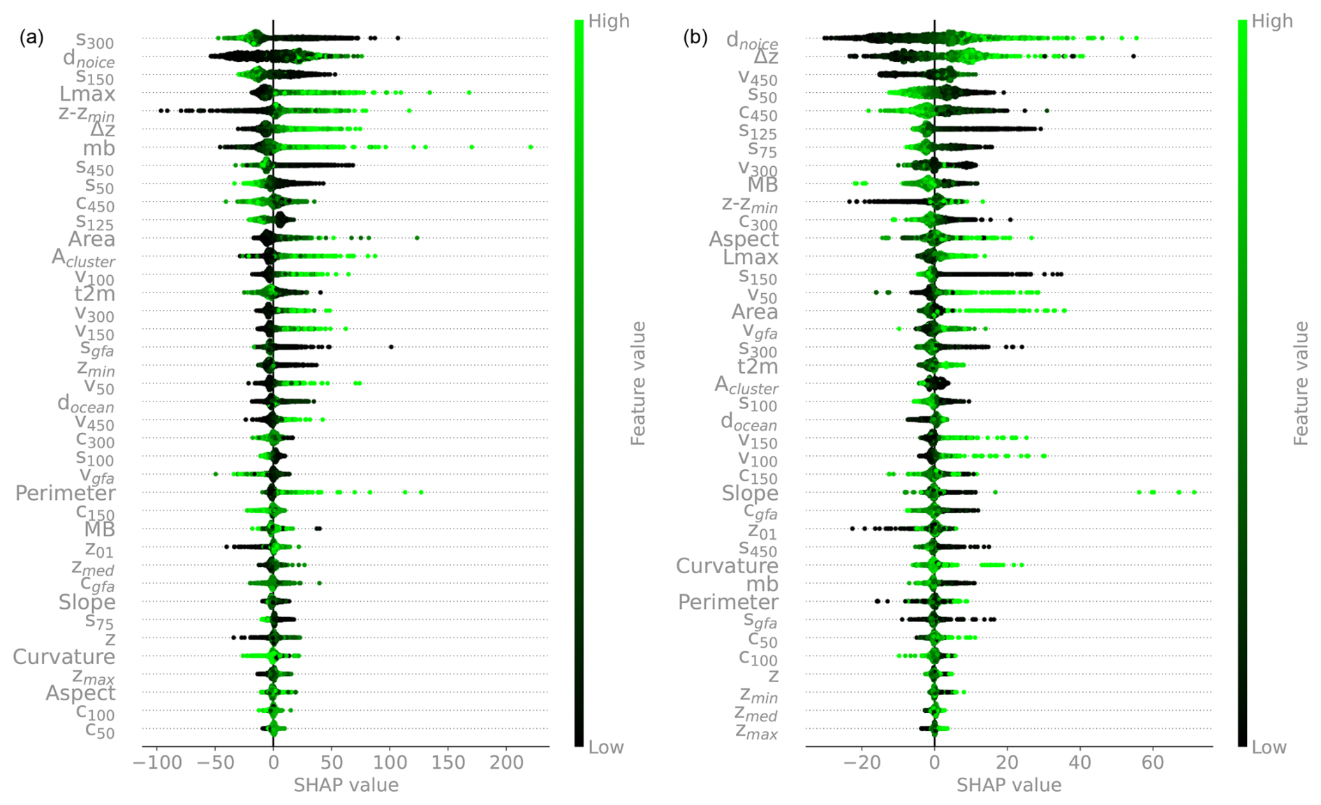
Figure 2 (a) SHAP analysis of n = 2000 random instances (each ice measurement instance is represented by a dot in each feature row). Features are ordered from top to bottom by decreasing mean absolute SHAP values: top features are more important. The horizontal coordinate indicates how the model output changes with respect to its baseline, in a positive or negative direction, and hence how predictive the features are. The colour bar reflects the normalized feature variability range. See Table 1 for the variable names. (b) The same analysis is carried out on a random set of points in RGI 11 (Central Europe). See Fig. A3 for the feature rankings based solely on absolute mean SHAP values.

2.5 Model

We utilize two gradient-boosted decision tree (GBDT) models (Friedman, 2001). A GBDT model consists of multiple additive decision trees and is trained iteratively. In each iteration, a new decision tree is added and tasked with fitting the residuals of the previous tree by minimizing an objective function. Training continues until a stopping criterion is met, either reaching a maximum number of iterations or detecting overfitting through a separate validation dataset. IceBoost is an ensemble model comprising two GBDT variants: XGBoost (Chen and Guestrin, 2016) and CatBoost (Prokhorenkova et al., 2018). Both models use a second-order Taylor approximation of the objective function and employ a depth-wise tree growth scheme. However, CatBoost builds symmetric trees, which tends to act as a regularizer against overfitting and handles categorical features natively without requiring one-hot encoding. We train both models independently using a squared loss, $l=(h-\widehat{h}{)}^{\mathrm{2}}$, where h represents the target thickness data from GlaThiDa and $\widehat{h}$ represents the modelled thickness. The IceBoost ensemble combines them by averaging their respective predictions.

Millan et al. (2022)Farinotti et al. (2019)

Table 2 IceBoost performance and comparison with existing models, as measured by RMSE, on a regional basis. All units are in metres. The numbers in parentheses refer to 1 standard deviation across n = 100 regional cross-validation runs. GTD: GlaThiDa.

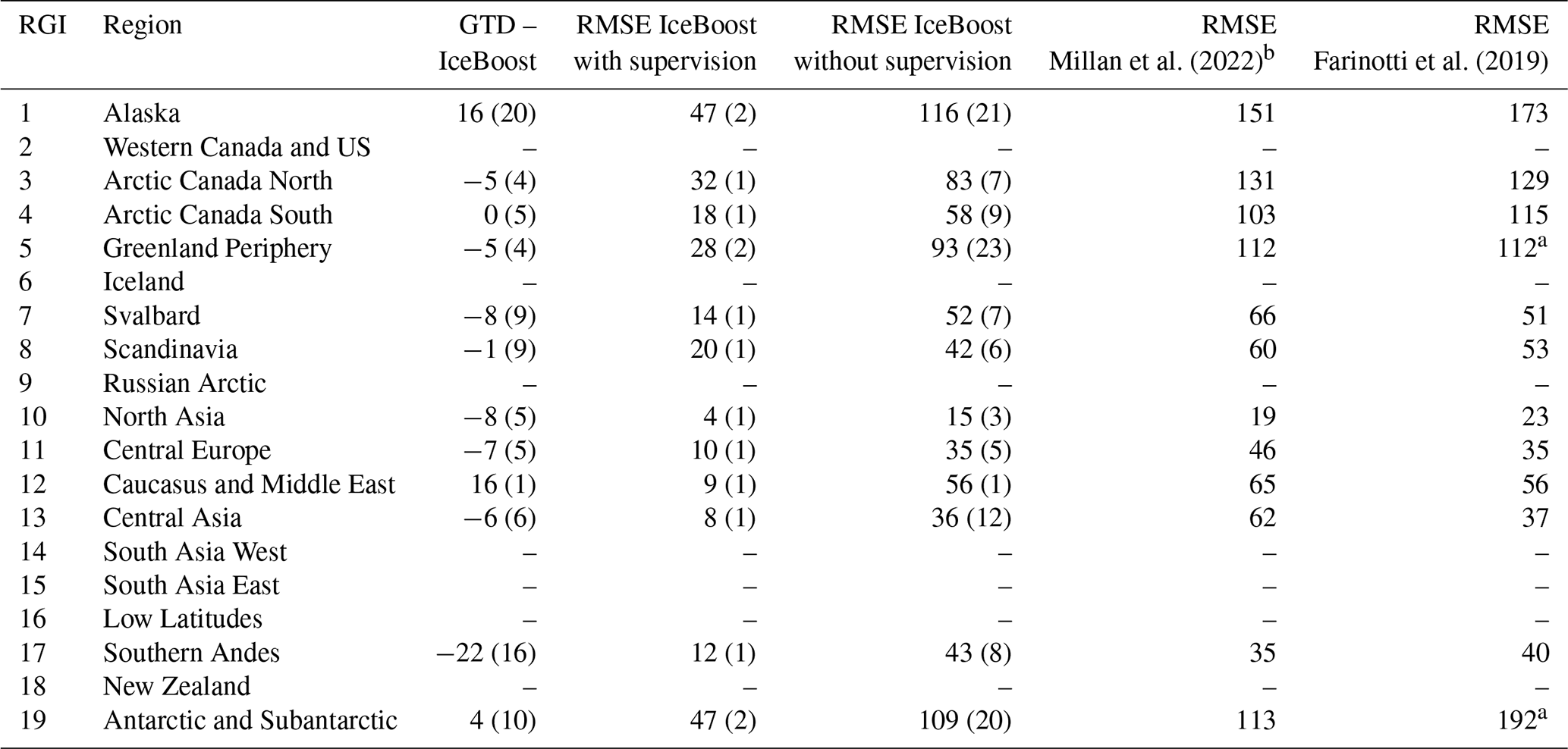
^a The evaluation is limited to glaciers with no connectivity to the ice sheet. ^b In RGI 5, this column integrates the results of BedMachine v.5 (Morlighem et al., 2022b). In RGI 19, this column refers to BedMachine v3.7 (Morlighem et al. 2022a).

Despite the different climates and glacier ice flow regimes in various regions, we decide not to specialize IceBoost regionally but rather to build one single model and optimize its hyperparameters globally. The decision is driven by the ease of deployment and the availability of certain features (particularly mass balance, temperature, and distance from the ocean) that can provide some regional context to the model. It should be noted that the model optimal parameters may reflect the imbalance of the training data among different regions, potentially making them slightly more biased towards polar regions where more training data are available. Potential solutions to specializing the model regionally would include optimizing the hyperparameters separately for each region and/or applying a heavier penalty within the regions of interest. We note that high thickness values are underrepresented in the training dataset (Fig. S1 in the Supplement). However, no significant bias is observed in regions with the thickest ice, such as Greenland and Antarctica (Table 2).

2.6 Model training, hyperparameter optimization, and performance

Hyperparameter tuning is conducted independently for XGBoost and CatBoost, both referred to as “model” for simplicity, and in an identical manner using a Bayesian hyperparameter optimization framework (Optuna; Akiba et al., 2019). The best parameters are determined by training each model over n = 200 trials. In each trial, a different set of hyperparameters is selected, the model is trained on an 80 % random split of the data, and the objective error loss is evaluated and monitored on the remaining 20 % split. Considering that the target ice thickness variable is not uniformly distributed (Fig. S1), to reduce the risk of overfitting to a particular data split, the 80 %–20 % random split is recreated every time the optimizer calls the objective function during a hyperparameter search. This approach effectively incorporates the dataset's variability as part of the noise. Its main advantage is that it helps identify hyperparameters that generalize well across different data splits, aiming for a more robust model. The trade-off is that randomizing the data splits in each trial introduces variability into the objective function, which can make convergence to the optimal hyperparameters more challenging. However, such variability in the loss is generally manageable within Bayesian optimization frameworks. To further prevent overfitting by reducing the model complexity, we enforce early stopping in each optimization trial (for both XGBoost and CatBoost). Early stopping is a form of regularization that halts training if performance on the 20 % split does not improve for a fixed number of rounds (n = 50). The best hyperparameters are identified as those selected in the trial for which the objective loss is minimized (Appendix A3). The XGBoost model is also optimized with respect to the following parameters that combat overfitting: lambda, alpha, and subsample.

We acknowledge that hyperparameter optimization is typically performed by leaving out a smaller third set for offline evaluation. However, we found that such evaluations were highly dependent on the data split, due to the stochasticity of the random split and the non-uniformity of the target variable. This dependency made the results less informative. For example, if Antarctic high-thickness data were included in the test set, the test set error would be disproportionately high. Consequently, no separate test set was created, and the entire dataset was allocated to training (80 %) and validation (20 %).

IceBoost performance is quantified by fixing the best set of hyperparameters, training the model, and evaluating its performance regionally using a cross-validation scheme (Table 2). We evaluate (i) the median of the residual distribution res = GTD − IceBoost and (ii) the root mean square error (RMSE) on a test set consisting of a 20 % random split of the regional data. Cross-validation involves training the model n = 100 times, each time randomizing the regional 20 % test split. Two different routines are considered to produce the 20 % test split. In the first routine (“with supervision”), the 20 % measurements are taken from glaciers where other data are considered for the 80 % training split. This approach allows the model to be trained on one glacier datum and tested on other locations within the same glacier (no data used for training are ever used for testing). In the second routine (“without supervision”), we impose a stricter constraint by creating the 20 % test from completely unseen glaciers. The model performance is reported in Table 2 for regions with sufficient data in the training set (Fig. 1). We cannot evaluate the model performance in regions 2, 6, 9, 14, 15, 16, and 18 due to too few or absent data. For regions 10, 12, 13, and 17, where the limited data are available, statistics are provided but are considered only indicative of regional performance. Nevertheless, a similar model behaviour is likely expected for regions that are geographically close and have a similar ice flow regime and similar mean thickness or feature values: 13–14–15 (extensive Himalayan glaciers), 6–7–9 (high-latitude glaciers and ice caps), and 8–11–12–18 (small- to medium-sized mountain glaciers). An example of one iteration of training without supervision is displayed in Figs. S3–S4.

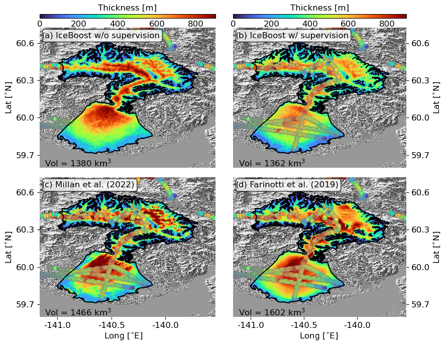
Figure 3 Modelling of Malaspina Glacier (RGI60-01.13696, Alaska) by IceBoost (this work, panels a and b), Millan et al. (2022) (c) and Farinotti et al. (2019) (d). IceBoost is trained without and with supervision in panels (a) and (b), respectively. The glacier ice volume difference between the two cases is 1.3 %. In panels (b), (c), and (d), the ground truth thickness data are represented as large circles. The Tandem-X EDEM hillshade is shown in transparency.

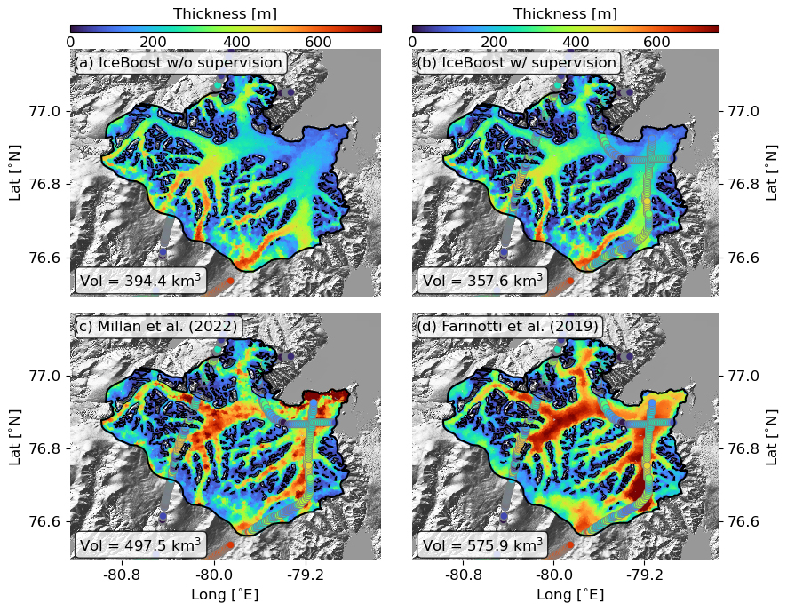
Figure 4 Modelling of Mittie Glacier (RGI60-03.01517, Arctic Canada North) by IceBoost (this work, panels a and b), Millan et al. (2022) (c), and Farinotti et al. (2019) (d). IceBoost is trained without and with supervision in panels (a) and (b), respectively. The glacier ice volume difference between the two cases is 9.5 %. In panels (b), (c), and (d), the ground truth thickness data are represented as large circles. The Tandem-X EDEM hillshade is shown in transparency.

The performance of XGBoost and CatBoost, evaluated individually on ground truth data, is comparable within 1σ statistical fluctuations, with neither consistently outperforming the other (Table S1). A qualitative comparison at inference time on selected glaciers suggests that the same conclusion holds, with similar predicted patterns even in the absence of ground truth data (Academy of Sciences ice cap shown in Fig. S2). We create IceBoost by taking an unweighted mean of XGBoost and CatBoost. Alternative approaches, such as applying regional weighting or per-glacier weighting based on feature explainability, could be explored but are left to future work.

Evaluated against ground truth data, IceBoost error is comparable to state-of-the-art global solutions outside polar regions and is up to 30 %–40 % lower in polar regions (Table 2). The much lower errors when training with supervision indicate that providing the model with glacier context proves to be beneficial. While this conclusion seems consistent on a regional scale, we find that, on a glacier-by-glacier basis, the model is not always sensitive to additional tie points, regardless of where the context is provided (further discussion in Sect. 4). On the Greenland and Antarctic peripheries, it is noteworthy that the Farinotti et al. (2019) model performance is only evaluated on glaciers not connected to the ice sheet. In Greenland (RGI 5), the statistics reported by Millan et al. (2022) combine their own shallow ice approximation for glaciers and ice caps not connected to the ice sheet, with Morlighem et al. (2022) kriging and mass conservation elsewhere. On the Antarctic periphery (RGI 19), as ground truth data are only found in the Antarctic continent (and none in the Subantarctic islands), the reported statistics refer entirely to BedMachine v.3.7 (Morlighem, 2022).

3 Model interpretability

To understand the relative strengths of the features for the model prediction, we carry out a feature ranking analysis using SHapley Additive exPlanations (SHAP; Lundberg and Lee, 2017). For the analysis we consider the XGBoost model. SHAP is a framework based on cooperative game theory where the goal is to equitably distribute the total gains to players (i.e. the model features) based on their individual contributions. A feature SHAP value reflects its marginal contribution to the model, specifically the change in the model's prediction when the feature is added or removed. Positive (negative) SHAP values indicate that the feature increases (decreases) the model prediction with respect to its average baseline (the sum of all SHAP values for a given instance equals the model's prediction for that instance), while SHAP absolute values represent the magnitude of the feature contribution to the model prediction, regardless of the direction.

A SHAP analysis is shown in Fig. 2 for a random global subset of n = 2000 training data points. Each instance is represented by a dot. The features are ordered from top to bottom by decreasing mean absolute values. That is, more important features are on top (a less informative but more compact visualization is shown in Fig. A3). The feature SHAP values are the x coordinates, while the feature values are represented in the colour bar. As an example, points with high distance-from-ice-free-region values typically have higher SHAP values. That is, they will push the model towards higher thickness predictions. For almost all features except for the slope and the curvature, higher feature values will lead to higher ice thickness predictions.

Local slopes and curvature are important features, highlighting the DEM quality as a crucial input for accurate glacier thickness estimates (see Appendix B5 for DEM-driven model artifacts). The elevation from the glacier minimum, rather than the absolute elevation above sea level, is found to be most informative.

The closest distance to ice-free areas is a powerful feature that often mirrors the ice thickness spatial distribution in continental valley glaciers. This feature retains its power even in large glacier systems with multiple nunataks (e.g. Fig. A1).

As is known from area–volume scaling models (Bahr et al., 2015), metrics for glacier extent (Area, L_max) are found to be powerful predictors. By providing regional context for different flow regimes and metrics of continentality, the 2 m temperature, T2m, and distance to the ocean d_ocean are found to be moderately informative. The local mass balance (mb) (Appendix A2) is also found to be relatively informative despite our simple elevation-based downscaling mass balance approach. We also acknowledge that most glaciers are currently out of equilibrium, likely resulting in the accumulation and ablation zones being altered by the climate signal. Ice velocity is found to be a major predictor, but, perhaps surprisingly, it is not as strong globally as those mentioned above. Possibly, the wide range of variability across over 3 orders of magnitude in velocity makes this information difficult to account for, in addition to, possibly, data uncertainty. The role of surface velocity is investigated further by training the model without velocity information. We find that the error increases by up to a maximum of 6 % for high-latitude regions, while no substantial difference is found elsewhere. We speculate that, at high latitudes, where more extensive glaciers are located, geodetic information becomes relatively less informative (low and uniform values of slope and curvature; absolute elevations of glaciers are less informative), increasing the ranking of the surface velocity. Since the largest ice volumes are stored at high latitudes, all velocity features are retained in the model.

Except for the metrics related to glacier size and glacier elevation difference Δz, all other glacier-integrated features (Slope, Aspect, and Curvature) are found to be relatively unimportant, including the glacier geodetic mass balance values mb (see also Appendix C). Overall, the analysis highlights the crucial importance of high-quality DEMs.

The analysis provides a general overview of the predicting power of the feature set by accounting for a random global set of training entries. A slight reshuffling of the feature ranking is expected, however, when evaluating glaciers individually (an example is discussed in Sect. 4) or regionally (e.g. RGI 11 in Fig. 2). The SHAP analysis proves very instructive for accessing the information gain provided to the model by each feature. It can be used to decide which features should be retained and which ones can be dropped without substantial loss of performance.

4 Model deployment

At deployment time, the model ensemble is tasked with producing a continuous glacier ice thickness solution. The pipeline consists in generating n discrete points randomly inside the glacier boundary and outside nunataks, calculating the feature vector x_n and querying the model locally: h_n=IceBoost(x_n). The feature vector x_n is calculated on the fly (Appendix B1). The glacier volume is calculated by Monte Carlo method (Appendix B3). An approximately continuous solution can be obtained in the limit ${lim}_{n\to \mathrm{\infty }}{h}_n\left({\mathit{x}}_n\right)$. Typically, n = 10 000 provides a good representation even for relatively big glaciers.

To investigate the effect of added supervision, we consider Malaspina Glacier (RGI60-01.13696). The glacier, located in coastal southern Alaska, is the world's largest piedmont glacier with an area of 3900 km². Its piedmont lobe is largely grounded below sea level. Measurements on this glacier are found in our training dataset. A recent campaign has vastly increased the number of measurements on the glacier and provided a detailed overview of the terminus thickness distribution and bedrock topography (see Fig. 5 in Tober et al., 2023).

We train the model with and without the available measurements included in the training dataset (hereafter referred to as “with and without supervision”). We note that, in contrast to a kriging technique, IceBoost does not use the data explicitly but rather adjusts its parameters at training time. The model trained without supervision predicts an ice thickness of up to 700–800 m at the terminus and in the other, deepest parts of the glacier (Fig. 3a). Next, we include the measurements in the training set and train the model with supervision. The model output changes drastically at the terminus (Fig. 3b), with the solution values closer to the ground truth, although the model still struggles to fully capture the high thickness values that correspond to localized deep subglacial channels found by radar surveys (Tober et al., 2023). Note that the solution changes in other parts of the terminus as well and also relatively far from the data. Training IceBoost with supervision greatly improves the model skill, suggesting that a significant advantage compared to existing approaches is achieved when data are available by (i) improving the general model performance by increasing the training data and (ii) improving the prediction on individual glaciers. While it is not trivial to understand why IceBoost prediction without supervision deviates from the ground truth for Malaspina Glacier, the model error is consistent with what has been found in this region at cross-validation (RGI 1, Table 2). The RMSE evaluated on ground truth data (n = 588) for this glacier is 147 m when the model is trained without supervision. Incorporating supervision with 20 % of the data reduces the RMSE to 31 m on the remaining 80 %, representing a 4.7-fold improvement. This experiment also shows that, although the model does not explicitly account for dependence between points (in contrast to a neural network structure), it produces a meaningful covariant pattern in both cases.

The same analysis is carried out for Mittie Glacier, a large and surge-type glacier in Arctic Canada North (Fig. 4). The RMSE is 68 m when training without supervision and 27 m with supervision, a reduction by a factor of 2.5 – approximately half the improvement observed for Malaspina Glacier. The comparison would suggest that not all modelled glaciers benefit equally from added supervision. We speculate that the improvement in model performance obtained with supervision is likely attributable to the inclusion of high-thickness data (and/or out-of-distribution feature values), which provide valuable information for modelling deep glaciers.

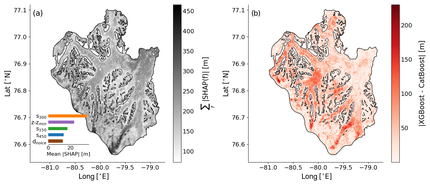
Figure 5 (a) Sum of absolute SHAP values of all features, calculated for Mittie Glacier. Higher (lower) values indicate greater (lesser) contributions from the feature set to the model. The top-five features are displayed in the inset, ranked from most important to least important by decreasing mean SHAP values. (b) Absolute difference between the XGBoost and CatBoost individual modules. The reader is referred to Fig. 4 for the geographical setting of the glacier.

To assess how the feature set influences the model prediction, we conducted a SHAP analysis of Mittie Glacier, evaluating feature SHAP values using the XGBoost module (Figs. 5 and 6). At each point, the sum of all feature SHAP values, ${\sum }_f\left|\mathrm{SHAP}\right(f\left)\right|$, reflects the overall contribution of the feature set to the model prediction (Fig. 5a). On Mittie Glacier, the feature set provides the most information in the deep ice streams of the south and at the marine terminus in the north-east. Differences between individual XGBoost and CatBoost predictions reach up to 150–200 m in the deepest regions (Fig. 5b). These differences mimic the IceBoost-averaged output (Fig. 4b). Averaged across the whole glacier, the five most important features (inset in Fig. 5a) are the slope (s₃₀₀, s₁₅₀, and s₄₅₀), the elevation above the glacier base ($z-z_{min}$), and the distance to ice-free regions (d_noice). The spatial variability in SHAP values reveals the areas where each feature contributes most (Fig. 6). The slope field smoothed with the widest kernel (s₄₅₀) is particularly informative near broad, flat glacier streams, while the slope smoothed with the smallest kernel (s₁₅₀) provides value over the steep, mountainous terrain located in between nunataks. The d_noice feature is also most informative near nunataks, whereas the elevation above the base ($z-z_{min}$) is especially valuable at the marine terminus and less so elsewhere. While the IceBoost model does not inherently provide an uncertainty estimate of predicted ice thickness, valuable insights can be derived by using the Shapley analysis on the feature set and to some extent by comparing the separate predictions of XGBoost and CatBoost.

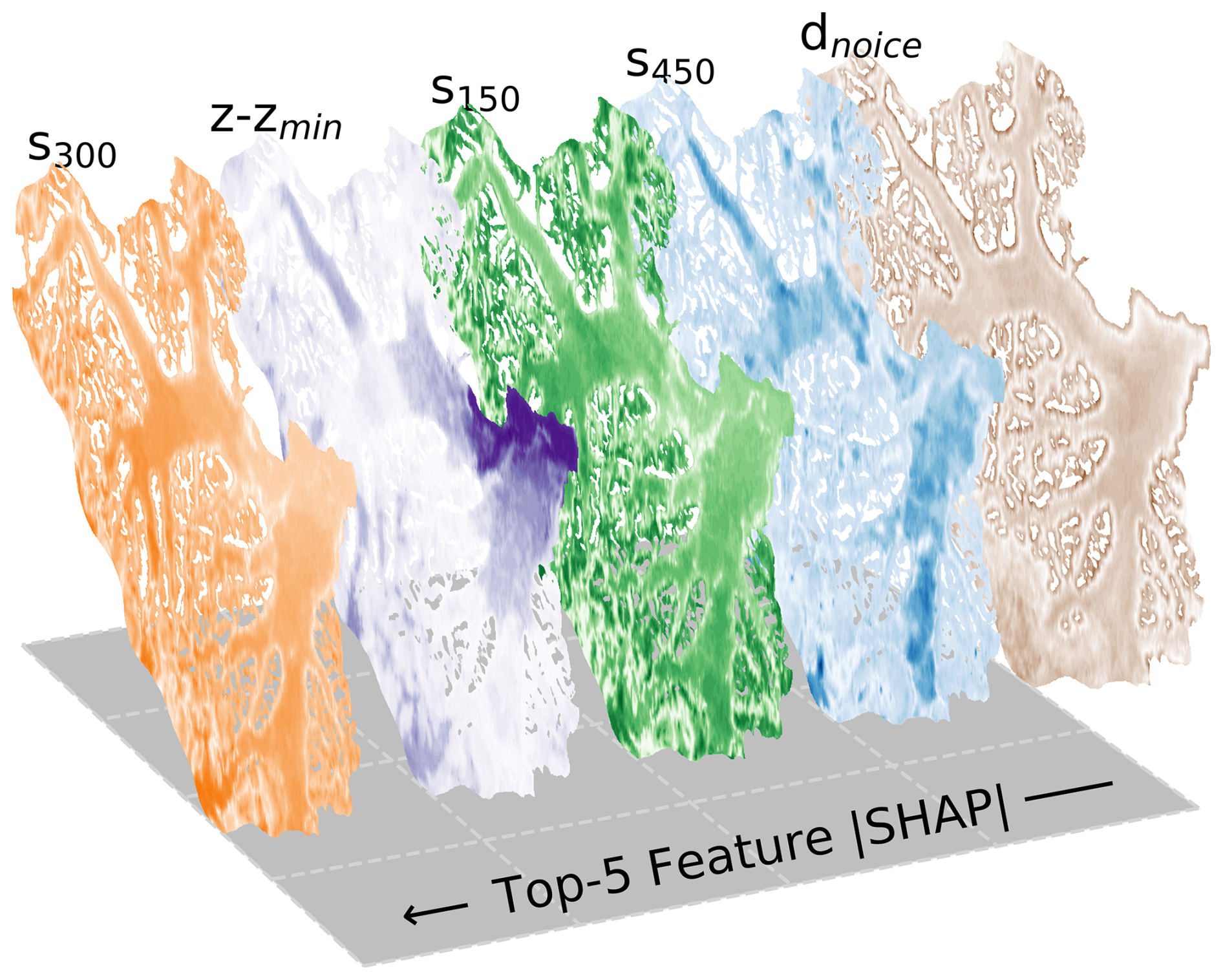
Figure 6 Absolute SHAP spatial variability of the top-five ranked features, calculated for Mittie Glacier. The colours range from white (low values) to saturated (high values). d_noice is important close to the glacier ice-free regions. The slope features s₁₅₀, s₃₀₀, and s₄₅₀ show similar patterns, with the widest 450 m slope more informative on the broad ice rivers and less valuable elsewhere. The $z-z_{min}$ feature is very informative close to the marine terminus.

The spatial resolution of the IceBoost model is considered hereafter. The input features are extracted from products with varying resolutions (Table 1). For example, the satellite products range from 30 m (DEM) to 250 m for surface velocity fields over the ice sheets. Convolution with various kernels of different sizes is also implemented when generating the features, enlarging the receptive field. Other features are per-glacier constants. The minimal spatial variation of the thickness maps generated by IceBoost, loosely referred to as the model resolution, is evaluated by visually assessing the predictions (examples in Fig. 7), and it is estimated to be ≃ 100 m. The model has neither the capabilities (it is not trained to) nor the resolution to predict smaller-scale basal features, unless their fingerprints are clearly reflected on the surface.

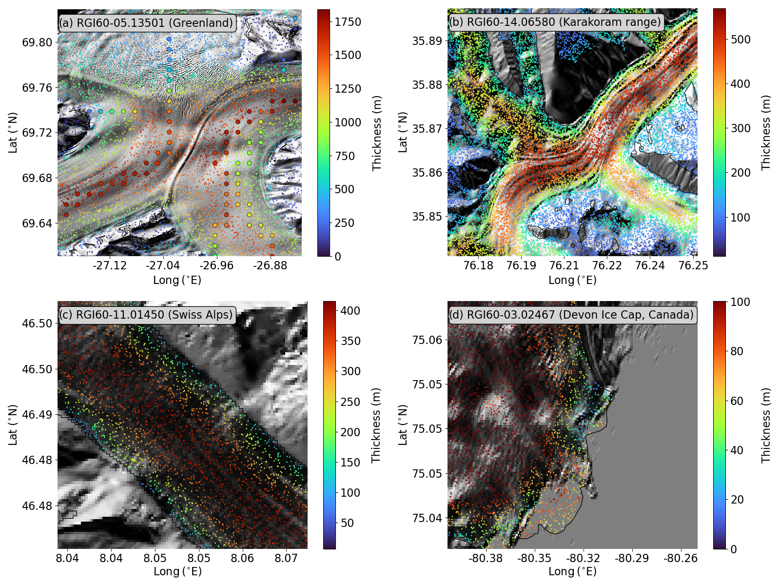
Figure 7 IceBoost-modelled glaciers at different spatial scales, overlaid on the Tandem-X EDEM hillshade. The small circles reflect the modelled ice thickness evaluated at random locations. In panel (a) the ground truth thickness data are represented as large circles.

We note that the model predicts at times rather fine-grained details in ice thickness, such as transitions close to ice shelves or in the proximity of high-elevation gradients (Fig. 7).

An extensive comparison between IceBoost and other models can be found in the Supplement (see the “Code and data availability” section) for 190 glaciers. For each 1 of the 19 RGI regions, n = 10 glaciers are modelled with IceBoost and compared to Millan et al. (2022) or BedMachine (whenever applicable, RGI 5: Morlighem et al., 2022, and RGI 19: Morlighem, 2022) and the ensemble of Farinotti et al. (2019).

5 Applications, improvements, and limitations

The ice thickness maps produced by IceBoost have significant potential in numerical modelling of future glacier evolution by providing a modern initial condition. Valuable insights can also be gained by utilizing IceBoost-derived maps compared to outputs from other inversion techniques, such as those of Millan et al. (2022) and Farinotti et al. (2019). A notable advantage of a machine learning model operating on tabular data is its flexibility in predicting point estimates of other variables, such as surface ice velocity or mass balance, by setting them as a training target. In these cases, ice thickness, if known, can serve as an additional input feature. Ice velocity maps (or mass balance) can be generated from scratch or used to fill gaps in existing products. Additionally, modelling the ice thickness of past glaciers can be explored, if their geometry is known, by leveraging knowledge of past feature records or using present-day features under specific assumptions.

Improvements to IceBoost can be explored by expanding the training dataset, both in the number of entries and the inclusion of more informative features. Prioritizing an increase in high-thickness data would be particularly beneficial. Ensembling with other machine learning models, such as a multi-layer perceptron, may further enhance performance by reducing point estimate error and improving the smoothness of the output solution, which is an important factor in numerical modelling. Additionally, implementing or running in parallel other machine learning schemes that generate probability distributions as output (e.g. NGBoost; Duan et al., 2020) could yield valuable uncertainty maps alongside predictions.

Enhancing the quality of the products used to generate the features, particularly the DEM, will certainly improve the model. Artifacts in the input DEM are the primary source of errors in the generated thickness maps. They are directly reflected in the model outputs, leading to visible inaccuracies in the proximity of the artifact (Fig. B3). Artifacts can also occur when the smoothing kernels applied to the input products are not sized appropriately. For instance, in the case of Glacier RGI60-19.00134 (Alexander Island, Antarctica, Fig. B3), the kernels used in this study may be too small to adequately capture and remove the elevation roughness present at the spatial scales of this glacier (∼ 4000 km²). This mismatch results in artifacts manifesting as (likely unrealistic) high ice thickness gradients (Fig. B3).

6 Computational cost

The memory load for creating the training dataset is 80 GB, primarily due to the memory necessary to import, merge, and operate on the DEM tiles. Downgrading to Tandem-X 90 m would certainly reduce the computational cost at the expense of accuracy. Model training and deployment can be done on either a GPU or a CPU. Model training requires a few minutes. The inference phase requires generation of the feature vector on the fly and querying of the model. The former requires between 1 s and 1 min for the most complex glaciers, almost independently of the choice of the number of points to generate (10⁴–10⁵). The latter is faster and requires approximately 10⁻¹ s per glacier. The feature generation dominates the computational cost, and parallelization with multiple processors is implemented in the model for regional simulations. For higher spatial details, the point density can be selectively increased locally up to O(10⁵). We recommend not increasing n above a million points as the information gain is limited by the model resolution (≃ 100 m). The hard disk memory recommendation is 500 GB. All of Earth's glaciers can be run conservatively on a 1 TB hard disk, 128 GB of RAM, and 1–20 CPUs. Unless feature calculation is moved to a GPU (e.g. RAPIDS Development Team, 2023), a graphics card is deemed unnecessary since the time overhead of data transfer surpasses the benefit of a marginally faster model query on a GPU.

7 Conclusions

To the best of our knowledge, IceBoost is the first global machine learning model capable of predicting ice thickness at arbitrary coordinates, enabling the creation of distributed ice thickness maps for glaciers worldwide. The model operates using a set of 39 numerical features; its parameters are optimized globally. The model error is similar to state-of-the-art models in mid- to low-latitude glaciers and is up to 30 %–40 % lower at high latitudes. However limited, the comparison with BedMachine also demonstrates the skills of the machine-learned approach in the ice sheet peripheries. As is typical of machine learning methods, the model performance is expected to improve by increasing the training dataset's size. Data from future measurement campaigns should be integrated into the training dataset. The large amount of training data available at high latitudes and the model errors in these regions suggest that, for our modelling approach, providing more data is more beneficial than providing more accurate data. Providing supervision (i.e. measurements) further reduces the model error by a factor of roughly ≃ 2 to 3. Measurement campaigns targeting deep ice zones would prove extremely beneficial for improving IceBoost estimates of ice volumes. However, we find that not all glaciers benefit equally from added supervision on an individual basis. With the exception of DEMs which are available at high resolution and increasing accuracy, our modelling approach is not hard-constrained by the availability of a specific input feature, notably ice velocity. Ice velocity improves the model by up to 6 % at high latitudes, though no improvement is found elsewhere. Despite its marginal impact, this area holds the majority of Earth's ice volume. The most informative features are the distances to ice-free regions, surface slopes, surface curvature, and metrics of glacier size. An improved mass balance feature will likely improve the model performance. We consider that our current local mass balance feature is only a simplified estimate. Our machine learning approach is fully data-driven, with its primary advantage being the ability to learn directly from data. However, deeper insights can be achieved by integrating physical principles into machine learning systems. Research in this direction would be a logical step forward.

Appendix A: Training features

A1 Glacier length (L_max) and distance from ice-free regions (d_noice)

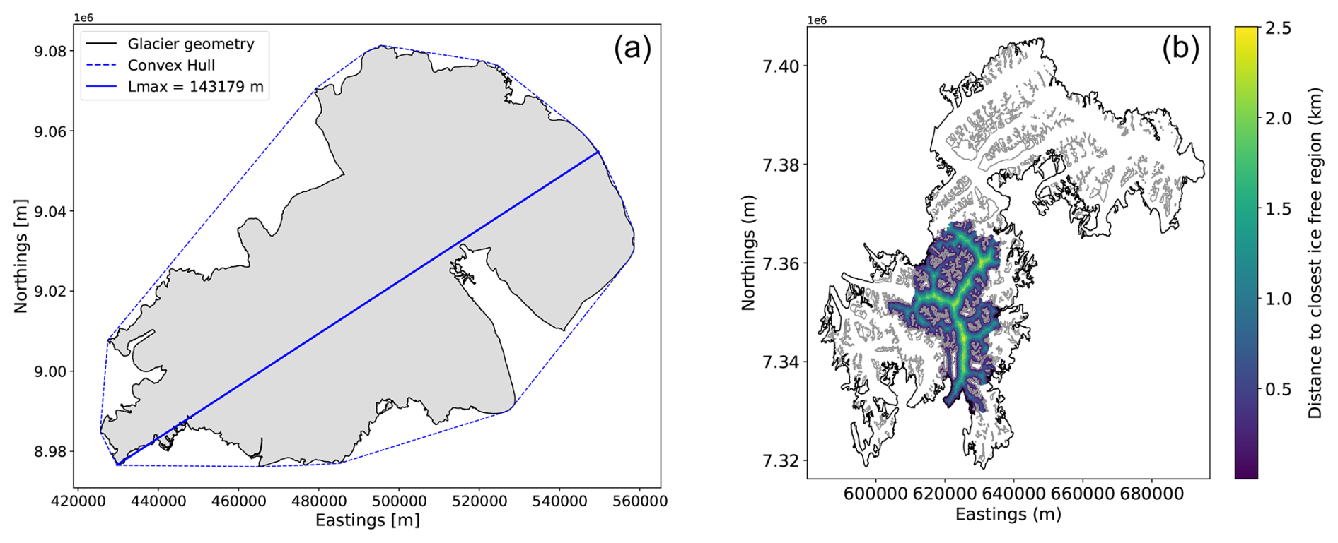
Figure A1 (a) RGI60-10315 glacier length (L_max). (b) RGI60-05.13995 glacier feature d_noice. The cluster external geometry with ice divides removed is shown in black. All cluster nunataks are shown in grey.

A2 Mass balance

A2.1 Polar ice sheet peripheries

In addition to glacier-averaged mass balance data from Hugonnet et al. (2021), we inform the model with local mass balance values. For the Greenland and Antarctic peripheries, we leverage the RACMO2 (Noël et al., 2018) product versions, downscaled, respectively, to 1 km (Noël and van Kampenhout, 2019) and 2 km (Noël et al., 2023). Before linearly interpolating the mass balance fields, we (i) compute the time average over the 1961–1990 and 1979–2021 time periods and (ii) fill some gaps in the dataset by convolving with Gaussian kernels of 1 and 2 km, respectively. A few gaps still remain in the mass balance fields in some areas and glaciers (Subantarctic islands and a few glaciers off the coasts of the Antarctic Peninsula) not covered by these datasets. For these areas, as well as for all the other glaciers, we use the approach described below.

A2.2 Glaciers outside polar ice sheets

For all glaciers outside the Greenland and Antarctic peripheries, we use the 2000–2020 mean glacier-integrated mass balance values from Hugonnet et al. (2021) and estimate the local variability by downscaling using approximate elevation–mass balance rates. In particular, for all glaciers within the same region, we assume a linear variation of mass balance with elevation:

$$\begin{array}{}\text{(A1)}& y=s\cdot h+q,\end{array}$$

where y is the mass balance and h is the elevation. s expresses the rate of change in the mass balance with elevation, while q reflects the mass balance at zero elevation. For any pair of glaciers,

$$\begin{array}{}\text{(A2)}& {\displaystyle }{y}_{\mathrm{1}}=s_{\mathrm{1}}\cdot h_{\mathrm{1}}+q_{\mathrm{1}},\text{(A3)}& {\displaystyle }{y}_{\mathrm{2}}=s_{\mathrm{2}}\cdot h_{\mathrm{2}}+q_{\mathrm{2}}.\end{array}$$

By using the glacier mean values $\mathrm{mb}=\stackrel{\mathrm{‾}}{y}$ from Hugonnet et al. (2021) and further assuming that for close glaciers $s_{\mathrm{1}}=s_{\mathrm{2}}=m$ and $q_{\mathrm{1}}=q_{\mathrm{2}}=q$, we obtain

$$\begin{array}{}\text{(A4)}& {\displaystyle }s={\displaystyle \frac{{\mathrm{mb}}_{\mathrm{1}}-{\mathrm{mb}}_{\mathrm{2}}}{\stackrel{\mathrm{‾}}{h_{\mathrm{1}}}-\stackrel{\mathrm{‾}}{h_{\mathrm{2}}}}},\text{(A5)}& {\displaystyle }q={\mathrm{mb}}_{\mathrm{1}}-s\stackrel{\mathrm{‾}}{h_{\mathrm{1}}}={\mathrm{mb}}_{\mathrm{2}}-s\stackrel{\mathrm{‾}}{h_{\mathrm{2}}}.\end{array}$$

For a given glacier i, compute its mean rate s_i by extending the calculation in Eq. (A4) to all the other glaciers in the region j≠i, weighting the mean by the inverse of the glacier distances:

$$\begin{array}{}\text{(A6)}& {\displaystyle }{s}_i={\displaystyle \frac{\sum _{i\ne j}\frac{\mathrm{\Delta }{\mathrm{mb}}_{ij}}{\mathrm{\Delta }{h}_{ij}}\cdot \frac{\mathrm{1}}{d_{ij}^{\mathrm{2}}}}{\sum _{i\ne j}\frac{\mathrm{1}}{d_{ij}^{\mathrm{2}}}}},\text{(A7)}& {\displaystyle }{q}_i={\mathrm{mb}}_i-s_i\stackrel{\mathrm{‾}}{h_i},\end{array}$$

where $\mathrm{\Delta }{\mathrm{mb}}_{ij}={\mathrm{mb}}_i-{\mathrm{mb}}_j$ and $\mathrm{\Delta }{h}_{ij}=\stackrel{\mathrm{‾}}{h_{\mathrm{1}}}-\stackrel{\mathrm{‾}}{h_{\mathrm{2}}}$ are the differences in glacier mass balance and average elevation between glacier i and some glacier j, while d_ij is the distance between the two glacier centre values.

As an example, the distribution of (s_i, q_i) calculated for all glaciers in RGI 11 (Central Europe, 3927 glaciers) is shown in Fig. A2.

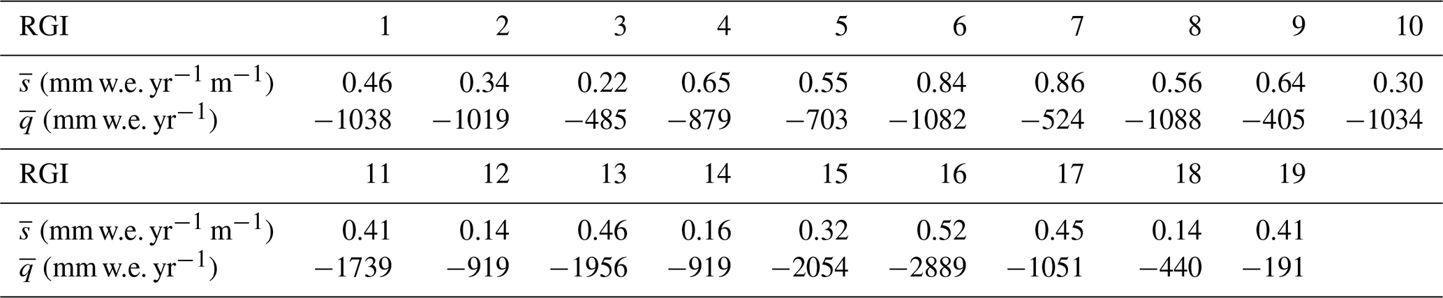
To compute mass balance maps for each glacier in each region, we use the regional mean values $\stackrel{\mathrm{‾}}{s}$ and $\stackrel{\mathrm{‾}}{q}$ listed in Table A1.

Using this method, we can replicate the glacier-integrated mass balance values (Hugonnet et al., 2021) within a factor of ≈ 2–3. Given all the hypotheses made, we consider our downscaling approach to be an attempt to provide the model with crude, yet local, mass balance approximations. An analysis of the impact of uncertainties in ($\stackrel{\mathrm{‾}}{s}$, $\stackrel{\mathrm{‾}}{q}$) on the modelled glacier volumes is presented in Appendix D.

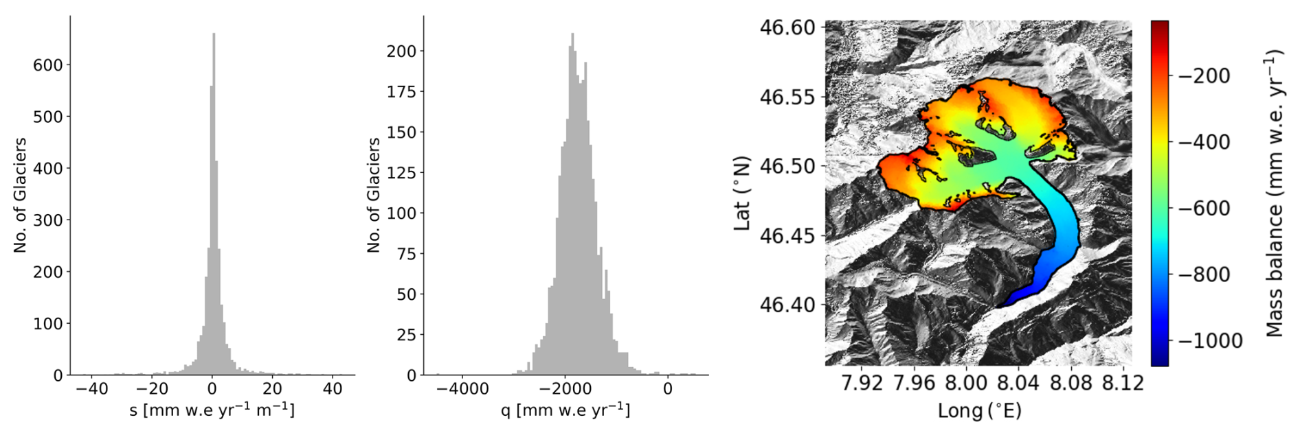
Figure A2 Distribution of (s_i, q_i) for RGI 11 along with the mass balance distribution for the Aletsch Glacier.

Table A1 Regional values of $\stackrel{\mathrm{‾}}{s}$ and $\stackrel{\mathrm{‾}}{q}$.

A3 IceBoost hyperparameters

The best XGBoost hyperparameters found during the Bayesian optimization pipeline are tree_method=hist, lambda=76.814, alpha=76.374, colsample_bytree=0.9388, subsample=0.741501, learning_rate=0.079244, max_depth=20, min_child_weight=19, and gamma=0.18611. We use 1000 trees (num_boost_round) with early_stopping_rounds=50. For CatBoost, iterations=10 000, early_stopping_rounds=50, depth=6, and learning_rate=0.1. For the parameter description, we refer to the XGBoost documentation at https://xgboost.readthedocs.io/en/stable/parameter.html (last access: 16 October 2024) and the CatBoost documentation at https://catboost.ai/en/docs/concepts/parameter-tuning (last access: 16 October 2024).

A4 Mean absolute SHAP values

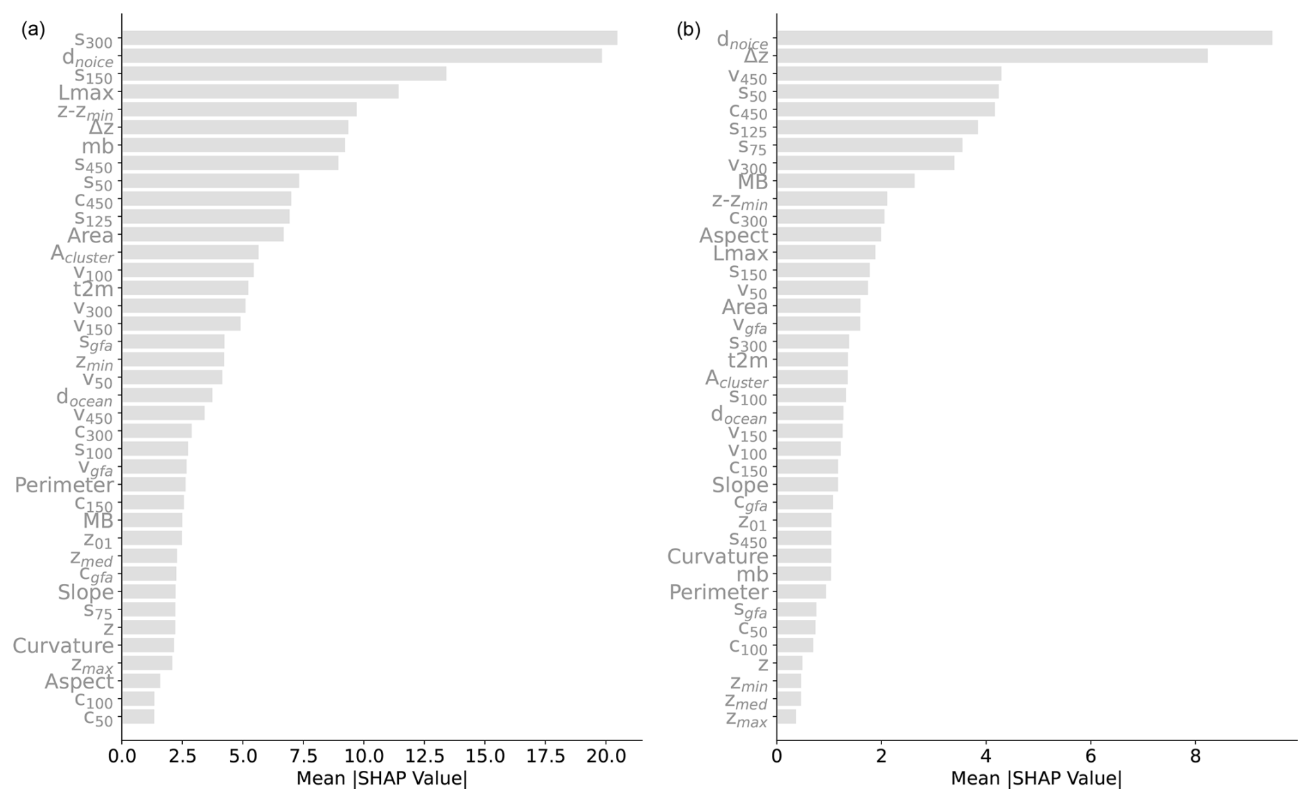
Figure A3 Feature ranking: the ranking of each feature is taken to be the mean absolute shape value for that feature over n = 2000 random samples (a) and over n = 2000 samples from Central Europe (RGI 11, b).

Appendix B: Model inference

B1 Fetching features on the fly

At inference time, the features are generated on the fly following the same pipeline described for the creation of the training set. As an example, Fig. B1 shows the extraction of the v₅₀ feature for n = 1500 random points.

Figure B1 Pipeline for feature generation at inference time. (a) Ice velocity (v₅₀, from Joughin et al. (2016) over glacier RGI60-05.13501 in East Greenland). (b) Feature calculated for n = 1500 random points.

B2 Feature imputation policies

Feature imputation is needed whenever any feature is not available, either for the creation of the training dataset or at inference time. Unless specified, we adopt the same policy in both cases. Hereafter we describe the imputation policies for ice velocity and mass balance.

B2.1 Ice velocity

No imputation is implemented at training time: if any velocity feature is missing at any point, the point is not included in the training dataset. This condition occurs if the training point falls outside the velocity field (old measurement or measurement inside a nunatak or incomplete velocity coverage) or if it is too close to the geometry such that the interpolation fails. At inference time, complete velocity feature coverage is required as input for the model. A three-layer progressive policy is implemented to fill any missing data and ensure complete coverage of all velocity features: (i) kernel-based interpolation using a fast Fourier transform convolution and Gaussian kernels, (ii) glacier-median imputation, and (iii) regional-median imputation.

B2.2 Mass balance

• Glacier-mean values: for glacier IDs listed in RGI v.62 but not present in the Hugonnet et al. (2021) mass balance dataset, which is tied to the RGI v.6 glacier dataset, we impute a regional median value. To be able to use the Hugonnet et al. (2021) dataset for glaciers in RGI v7, we link all glacier IDs from RGI v6 to RGI v7 by finding the glacier in RGI v7 that has the maximum area overlap with any RGI v6 glacier. If no glacier is found, we impute a regional median value from RGI v6.

• The RACMO products used for Greenland and Antarctica do not cover some glaciers located on islands proximal to the ice sheets. Among them are almost all glaciers from the sub-Antarctic islands. For these, we use the downscaling approach described in Appendix A2.2.

B3 Glacier volume calculation

The glacier volume is approximated by Monte Carlo method as $V_{\mathrm{gl}}=A_{\mathrm{gl}}{N}^{-\mathrm{1}}\cdot {\sum }_{x,y}h(x,y)$, where A_gl is the glacier area, h(x,y) is the modelled thickness at point (x,y) inside the glacier, and N is the total number of generated points. This method, tested by comparing Farinotti's interpolated thickness values against their true values, allows us to quantify its error to be less than 1 %, even for the biggest glaciers. While N=10⁴ allows for a precise volume estimate, to better evaluate the spatial variability of the solution over scales of tens of metres, N can be increased to O(10⁵), depending on glacier size, or increased locally to target specific regions.

B4 Comparison with BedMachine Greenland

Figure B2 shows a comparison between IceBoost and BedMachine v5 (Morlighem et al., 2022) for a glacier with a direct connection to the ice sheet. Note the additional complexity of the fjord system predicted by IceBoost compared to BedMachine. While an extensive comparison with BedMachine is beyond the scope of this work, we highlight the potential of IceBoost on the ice sheet peripheries.

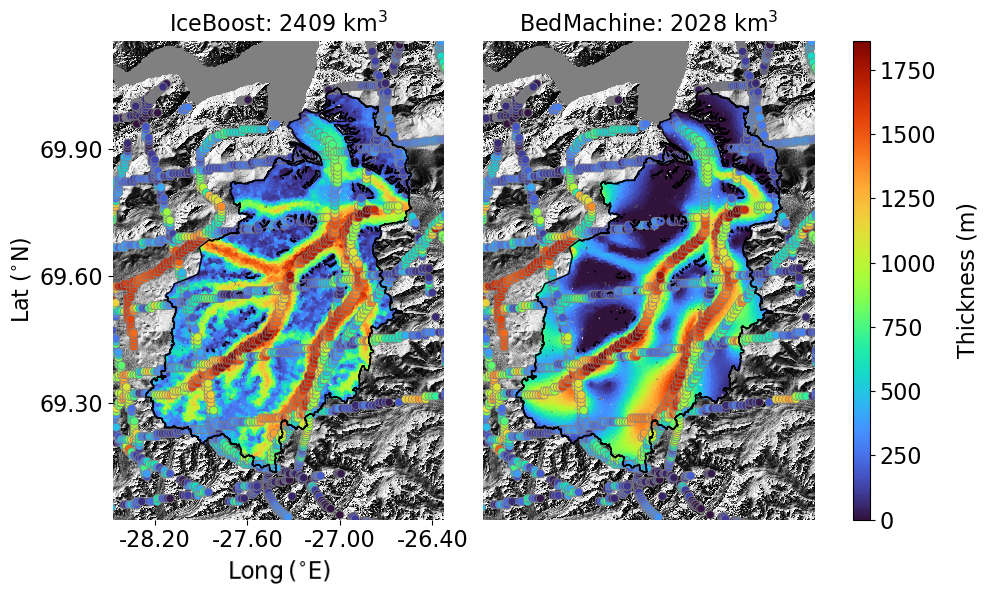
Figure B2 Glacier RGI60-05.13501 modelled by IceBoost and BedMachine v5 (Morlighem et al., 2022).

B5 Artifacts in the modelled output

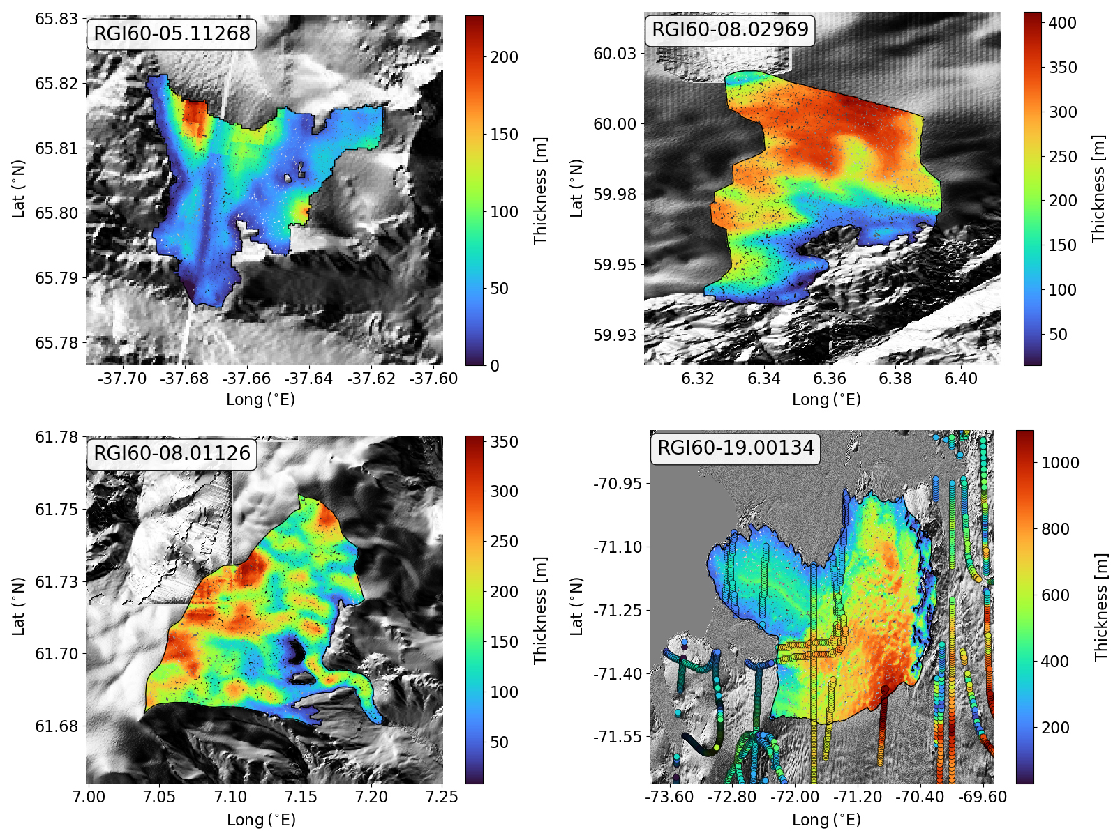
Figure B3 Modelled glacier ice thickness. Artifacts in the Tandem-X EDEM are visible for glaciers RGI60-05.11268, RGI60-08.02969, and RGI60-08.01126. The effects of such artifacts are visible in the modelled thickness map. Glacier RGI60-19.00134's modelled thickness shows some high-frequency noise that mimics the roughness of the surface.

Appendix C: Sensitivity of model outputs to the input glacier-integrated mass balance

We assess the model's sensitivity to input mass balance values (feature mb, imported from Hugonnet et al., 2021) using the Unteraargletscher (Switzerland; 46°34^′0^′′ N, 8°13^′0^′′ E) as a case study. This glacier was chosen due to extensive surveys conducted by Swiss glaciologists over decades, together with ground truth measurements. The reference mass balance value is −1.59 m w.e. yr⁻¹ (Hugonnet et al., 2021). IceBoost is run over a range of mass balance values from −4.0 to 4.0 m w.e. yr⁻¹, extending beyond realistic limits for this glacier and including the reference value −1.59 m w.e. yr⁻¹ (Fig. C1). Glacier volume shows limited dependence on mass balance, varying by at most 20 % across the entire range, with some predictions differing by less than 0.001 km³. In our model setup, glacier-integrated mass balance is a weak predictor of local ice thickness. This finding aligns with global results obtained from the variable ranking analysis of the training dataset (Sect. A4, Fig. A3).

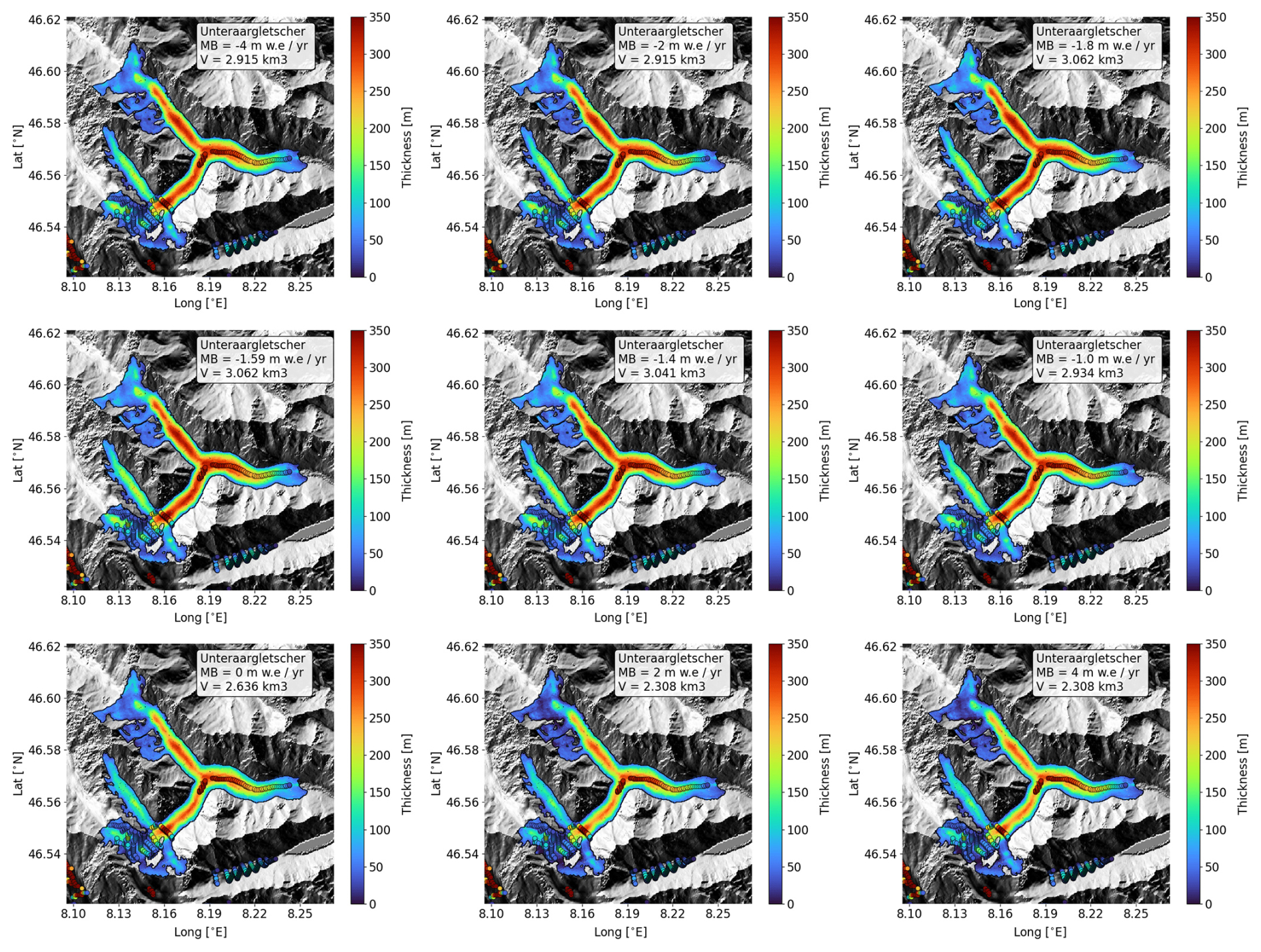
Figure C1 Unteraargletscher ice thickness modelled with different input mass balance values indicated in the insets. The reference mass balance for this glacier is −1.59 m w.e. yr⁻¹ (Hugonnet et al., 2021). The circles refer to ground truth data.

Appendix D: Sensitivity of model outputs to the input spatially distributed mass balance

The uncertainty in the inferred regional values of ($\stackrel{\mathrm{‾}}{s}$, $\stackrel{\mathrm{‾}}{q}$) used to calculate mass balance maps (feature mb; see Appendix A2.2) is investigated here. These parameters represent, respectively, the rate of change in the mass balance with elevation ($\stackrel{\mathrm{‾}}{s}$) and the mass balance at zero elevation ($\stackrel{\mathrm{‾}}{q}$). The parameters are calculated regionally, and hence all glaciers in the same region share the same values.

We analyse two glaciers in Switzerland: Unteraargletscher (46°34^′0^′′ N, 8°13^′0^′′É) and Aletsch (46°26^′32^′′ N, 8°4^′38^′′ E). For both glaciers, $\stackrel{\mathrm{‾}}{s}=\mathrm{0.41}$ mm w.e. yr⁻¹ m⁻¹ and $\stackrel{\mathrm{‾}}{q}=-\mathrm{1739}$ mm w.e. yr⁻¹ (Appendix A2.2). We conduct three Monte Carlo simulations with n = 500 iterations. For each set of simulations, random noise drawn from a Gaussian distribution is added to the $\stackrel{\mathrm{‾}}{s}$ and $\stackrel{\mathrm{‾}}{q}$ input variables, with widths of 10 %, 20 %, and 50 % of their nominal values. The resulting distributions of modelled output volumes are shown in Fig. D1, compared to the nominal values of 3.06 km³ (Unteraargletscher) and 14.4 km³ (Aletsch) obtained without added noise.

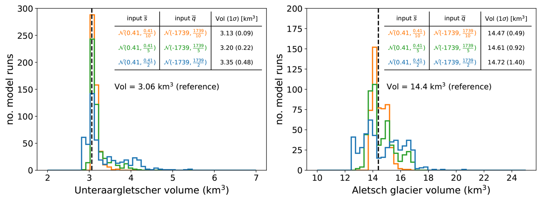
Figure D1 Monte Carlo simulations of modelled glacier volumes for Unteraargletscher and Aletsch, incorporating Gaussian noise into the input parameters ($\stackrel{\mathrm{‾}}{s}$ and $\stackrel{\mathrm{‾}}{q}$). Noise levels of 10 % (orange), 20 % (green), and 50 % (blue) are applied. These parameters are used to compute the spatially distributed mass balance (Appendix A2.2). The black line represents the modelled glacier volume without added noise.

For a 50 % uncertainty in $\stackrel{\mathrm{‾}}{s}$ and $\stackrel{\mathrm{‾}}{q}$, the modelled glacier volume changes, on average, by 9.5 % (Unteraargletscher) and 2.2 % (Aletsch), with variabilities of 14 % and 9.5 %, respectively. The total uncertainties, combining systematic and random components, are ±17 % for Unteraargletscher and ±9.8 % for Aletsch. With a 20 % uncertainty, the volume errors are ±8.2 % (Unteraargletscher) and ±6.4 % (Aletsch), while for a 10 % uncertainty they are ±3.7 % and ±0.5 %, respectively.

This sensitivity test, though limited to two glaciers in Central Europe, suggests that the error in the modelled glacier volumes due to uncertainty in the mass balance parameterization can be safely considered to not exceed 15 %.