The ensemble consistency test: from CESM to MPAS and beyond

The ensemble consistency test (ECT) and its ultrafast variant (UF-ECT) have become powerful tools in the development community for the identification of unwanted changes in the Community Earth System Model (CESM). By characterizing the distribution of an accepted ensemble of perturbed ultrafast model runs, the UF-ECT is able to identify changes exceeding internal variability in expensive chaotic numerical models with reasonable computational costs. However, up until now this approach has not seen adoption by other communities, in part because the process of adapting the UF-ECT procedure to other models was not clear. In this work we develop a generalized setup framework for applying the UF-ECT to different models and show how our specification of UF-ECT parameters allows us to balance important goals like test sensitivity and computational cost. Finally, we walk through the setup framework in detail and demonstrate the performance of the UF-ECT with our new determined parameters for the Model Across Prediction Scales-Atmosphere (MPAS-A), the substantially updated CESM atmospheric model, and realistic development scenarios.

1 Introduction

Scientific numerical computer models have existed for as long as modern computers. From test weather problems run on ENIAC (Easterbrook et al., 2011; Charney et al., 1950) to large-scale climate models run on some of the largest supercomputers in the world, these models have pushed the boundaries of computational resources and techniques. Ensuring correctness in these models as they evolve is key to having confidence in their predictions but is particularly difficult when considering the complexity of their code bases, the computational cost to run the models, and the chaotic dynamics often present. For instance, the Community Earth System Model (CESM) code base has been in development for over 25 years, contains over 2.5 million lines of code, exhibits strong chaotic behavior, and can easily require hundreds of thousands of core hours for a climate-scale model run (Danabasoglu et al., 2020).

Changes are constantly occurring between versions and implementations of a given numerical model. These changes might represent porting to a new computing cluster, a new compiler version or optimization, or changes to the code base itself. In short, these kinds of changes occur continuously in the normal course of model development and use. Identifying when these changes result in different scientific conclusions is a key part of software quality assurance. Exact definitions vary, but some would consider it to be part of “correctness” and “verification” tasks (Oberkampf and Trucano, 2008).

In strictly deterministic numerical models this task may appear to be relatively easy; one can compare the outputs of two model implementations directly and test for equivalence. This approach is referred to as bit-for-bit (BFB) equivalence, and historically this is indeed how correctness was ensured in weather and climate modeling (Easterbrook and Johns, 2009). However, requiring BFB equivalence can be quite onerous because of how many common changes may violate it. Bugs or programming mistakes will result in a BFB difference, but so too will porting to a new architecture (Rosinski and Williamson, 1997), changing software libraries or compiler versions, or making mathematically equivalent changes to the source code. And, if chaotic dynamics exist, what are initially small differences can quickly grow. As heterogeneous computing approaches become more common, like the use of GPUs, it is likely that BFB equivalence will become even more difficult, if not impossible, to achieve (see, e.g., Ahn et al., 2021).

Without BFB equivalence, distinguishing innocuous from scientifically meaningful changes has traditionally been a laborious task. For the CESM, testing involved the creation of numerous long climate runs (typically 400 years) using both the new and accepted model configurations. Those simulations would then be analyzed and compared by climate scientists. This approach required substantial computational and human resources. Because so many common changes can result in non-BFB changes, these costs were incurred frequently. The need for better verification and reproducibility tools has been noted repeatedly in scientific computing (see Gokhale et al., 2023; Clune and Rood, 2011).

Absent the ability to ensure BFB equivalence, and attempting to avoid analyzing multi-century model simulations by hand, the ensemble-based consistency test (ECT) was introduced in Baker et al. (2015) for use with the atmospheric portion of CESM. The ECT approach relies on the characterization of a reference numerical model configuration created with a large ensemble of perturbed initial conditions. After characterizing the reference configuration, a hypothesis test can be run to determine whether a small number of test model runs from a new configuration is “consistent” with the distributional characteristics of the reference configuration. The term “consistency” emphasizes the fact that some statistical form of correctness is still possible without BFB equivalence. A major practical improvement occurred by moving to ultrafast (hence UF-ECT) model runs, as described in Milroy et al. (2018). For UF-ECT, models were run for just 4.5 simulation hours (or nine time steps) compared to the 1-year-long runs in the original ECT work (in this work we will focus exclusively on the UF-ECT method). This approach provided both a quantitative and replicable approach for consistency testing while substantially reducing the computational cost. The ECT and UF-ECT approaches were made available as part of the PyCECT software library (Baker et al., 2015), a Python-based implementation available from GitHub (https://github.com/NCAR/PyCECT, last access: 3 April 2025) and have been incorporated into the CESM code base since 2016.

However, up to the present time, UF-ECT development has been closely intertwined with CESM. Configurable test parameters were specified based on the version of CESM at the time the method was created, sometimes in a fairly ad hoc way. In this paper we develop a generalized setup framework for applying the UF-ECT to different models. This setup framework is designed to specify test parameters such that they fulfill two main goals. The first is to ensure that the test is sensitive to changes throughout the model. This requires that the model is run long enough and characterized accurately enough that changes are detectable in the outputs. The second is to ensure the usability of the test by avoiding erroneous failures, whether they are caused by numerical issues or errors and biases resulting from inadequate samples. In this paper, we will examine the theoretical and statistical impacts of the test parameters as they relate to these goals, allowing model developers to utilize the UF-ECT with greater confidence.

The setup framework developed here should only have to be followed once as long as the overall structure and model size remain roughly the same. For example, developers could switch to using a new cluster as the accepted configuration without needing to again use the setup framework to determine UF-ECT parameters. However, if substantial new physics are added to a model, resulting in many new output variables, the test parameters may need to be updated, as we will explore later.

This paper is divided into four main sections. First, we provide an overview of the UF-ECT method and show how key test parameters can impact the method's performance. Second, we apply our setup framework to a different global atmospheric model, the Model Across Prediction Scales-Atmosphere (MPAS-A) (Skamarock et al., 2012), not used in previous ECT works. Third, we consider a recent version of the Community Atmosphere Model (CAM) in CESM, which, when measured by its number of default output variables, has roughly doubled in size since the UF-ECT was first developed. We investigate whether such substantial changes to CAM necessitate updating the UF-ECT test parameters and whether those parameters should work for multiple model resolutions. Finally, we perform a variety of experiments using UF-ECT with MPAS-A, demonstrating the effectiveness of our setup framework to specify appropriate test parameters.

2 UF-ECT overview

The UF-ECT was designed as an objective means of identifying statistically meaningful changes for expensive numerical models, where BFB equivalence is unreasonable and chaotic effects cause small changes to grow quickly. UF-ECT enables efficient consistency testing by characterizing the output distribution from a “reference” computer model to test new configurations of the model against. If the two configurations of the model are found to be statistically distinct, UF-ECT cannot tell us which version is actually correct, in the sense of matching the underlying equations or physics. For example, it is possible that a changed configuration of the model actually better approximates some underlying physical law. UF-ECT only attempts to answer the following question: is the new model configuration statistically distinguishable from the reference configuration?

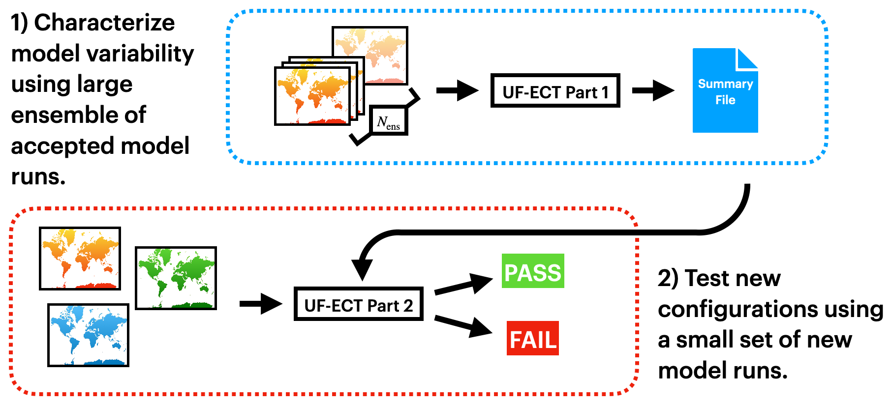
Figure 1 Diagram of the UF-ECT procedure. The test is designed so most work is done only once, when generating the reference ensemble. New model configurations can be tested with just three model runs.

A detailed description of the UF-ECT is included below, but at a high level it involves two parts. First, a large ensemble of perturbed model runs from a reference configuration is created and characterized in a lower-dimensional orthogonal space. Second, a small number of runs from a new test configuration are created and then used to determine whether the null hypothesis that the test configuration and the reference model configuration came from the same distribution can be rejected (Fig. 1).

The design of the UF-ECT achieves a few important goals. First, compared to relying on subjective human analysis, it is objective and does not require high levels of expertise in the scientific domain of question. Second, using short model runs makes ensemble generation computationally cheap. Third, the approach is designed to have most of the work, creating the large ensemble, done only once, requiring very little computational expense when new configurations are tested.

Distributions of numerical model outputs are created by slightly perturbing the initial conditions of the model, then running it forward for a relatively small time span and using those final instantaneous values. When used for CESM, this involved a 𝒪(10⁻¹⁴) perturbation to the initial temperature field. Other models could perturb a different variable as long as it is strongly coupled into the rest of the model, so model outputs quickly take on unique trajectories in state space. Previous works have even explored other sources of variability such as different compilers (Milroy et al., 2016). The spread of the perturbed ensemble relies on the same chaotic dynamics that prohibit BFB comparisons of outputs. How long to run the models is related to how quickly perturbations spread through the model and how well we can characterize the output distributions; this shall be addressed later.

The UF-ECT was initially designed for large spatial climate model codes. Characterizing model behavior when there are many output variables across multiple spatial dimensions has traditionally been difficult (though recent work has made progress by utilizing sparse graphical models and orthogonal basis vectors Krock et al., 2023). For UF-ECT, spatial variables defined at each grid cell are spatially averaged to one global mean value at each time slice (this includes averaging across the vertical component of any three-dimensional variables). The spatial averaging step of UF-ECT allows the subsequent assumption that output distributions of the global means can be estimated as Gaussian distributions due to the central limit theorem. With the large number of spatial outputs generally found in these models (on the order of 1 million grid points across three dimensions), this has proven a reasonable assumption.

Despite the loss of information incurred by spatial averaging, this has not been found to adversely affect the ECT approach during substantial use with CAM (shown across a wide variety of tests in Baker et al., 2015; Milroy et al., 2016, 2018). While modifications will likely result in new spatial distributions for model outputs, it appears very difficult to create a non-contrived change that does not also impact the spatial means in a detectable way. But, this may not always be the case. If a configuration change affects only the spatial distribution of an output field without modifying the average magnitude of that field, spatial averaging would prevent the test from being effective. This behavior was found in Baker et al. (2016) where spatial averaging ended up erasing the effect of configuration changes in a global ocean model, where there are relatively very few output variables to consider and very different spatial and temporal timescales from atmospheric models. Our recommended setup framework will help determine whether spatial averaging is appropriate if model developers are unsure.

A key step in the UF-ECT involves the transform of output variables using principal component analysis (PCA). Because large scientific numerical models often contain many related output variables, PCA is used to give us an orthogonal basis on which to compare model configurations, typically using fewer dimensions than the original output. Using PCA also enables the characterization of the relationship between variables, a key factor in the sensitivity of UF-ECT. For example, considered in isolation, one variable describing high rainfall and another describing zero cloud cover might both be “in distribution”. But, when considering the relationship between clouds and rain, such a combination would be quite unusual. PCA helps avoid the need for the high levels of model expertise necessary to distinguish related from unrelated output variables.

The use of PCA is one reason to exclude some variables before beginning the UF-ECT. Using constant or exactly linearly correlated variables can introduce numerical issues to the PCA step due to the resulting low-rank matrices (these are identified using a QR-factorization approach described in Sect. 3.3). Traditionally discrete variables have also been excluded to avoid any possible issues related to the assumption of continuous distributions. This requirement may be relaxed in future work but in our experience has not been onerous as most discrete variables have a related continuous variable that provides information about the same part of model behavior. For example, a vertical level index for the height of the tropopause is closely related to other continuous pressure variables.

Like other testing methods, the UF-ECT approach must strike a balance between sensitivity to true failures, meaning those that produce statistically meaningful changes in the model, and minimizing the number of tests that fail when they should actually pass, also known as the false positive rate (FPR). In our context, FPR is evaluated by determining the rate at which runs from the reference ensemble fail the test. If the test is not sensitive enough, it will not detect important changes impacting the output of the model. Conversely, if it is too sensitive, it will result in too many false positives, a frustrating result which could prevent model developers from wanting to use the approach at all. Hence, the approach presented in this paper works to balance these two characteristics to achieve the overall objective of the test.

Other approaches to correctness testing have been proposed and used in the scientific computing field, all attempting to address the chaotic variability of numerical models while maintaining reasonable computational cost. Some rely on the approach of quantifying perturbation growth over time (see, e.g., Rosinski and Williamson, 1997; Wan et al., 2017). Works like that of Mahajan et al. (2019a) (see also Mahajan et al., 2017, 2019b) employ an ensemble approach but do so in a symmetrical way where test and accepted ensembles are of a similar size. How to balance the cost of long runs and ensemble sizes is a common issue; for instance, Massonnet et al. (2020) use much smaller five-member ensembles than UF-ECT, but they are run for 20 years of simulated time. Similarly, approaches must decide whether to use a smaller subset of output variables of a model (like the 10 variables used in Wan et al., 2017) and whether to compare outputs with or without spatial averaging (like in Mahajan, 2021). The UF-ECT combination of asymmetrical ensemble sizes, short model runs, and PCA transforms appears to still be unique in the literature.

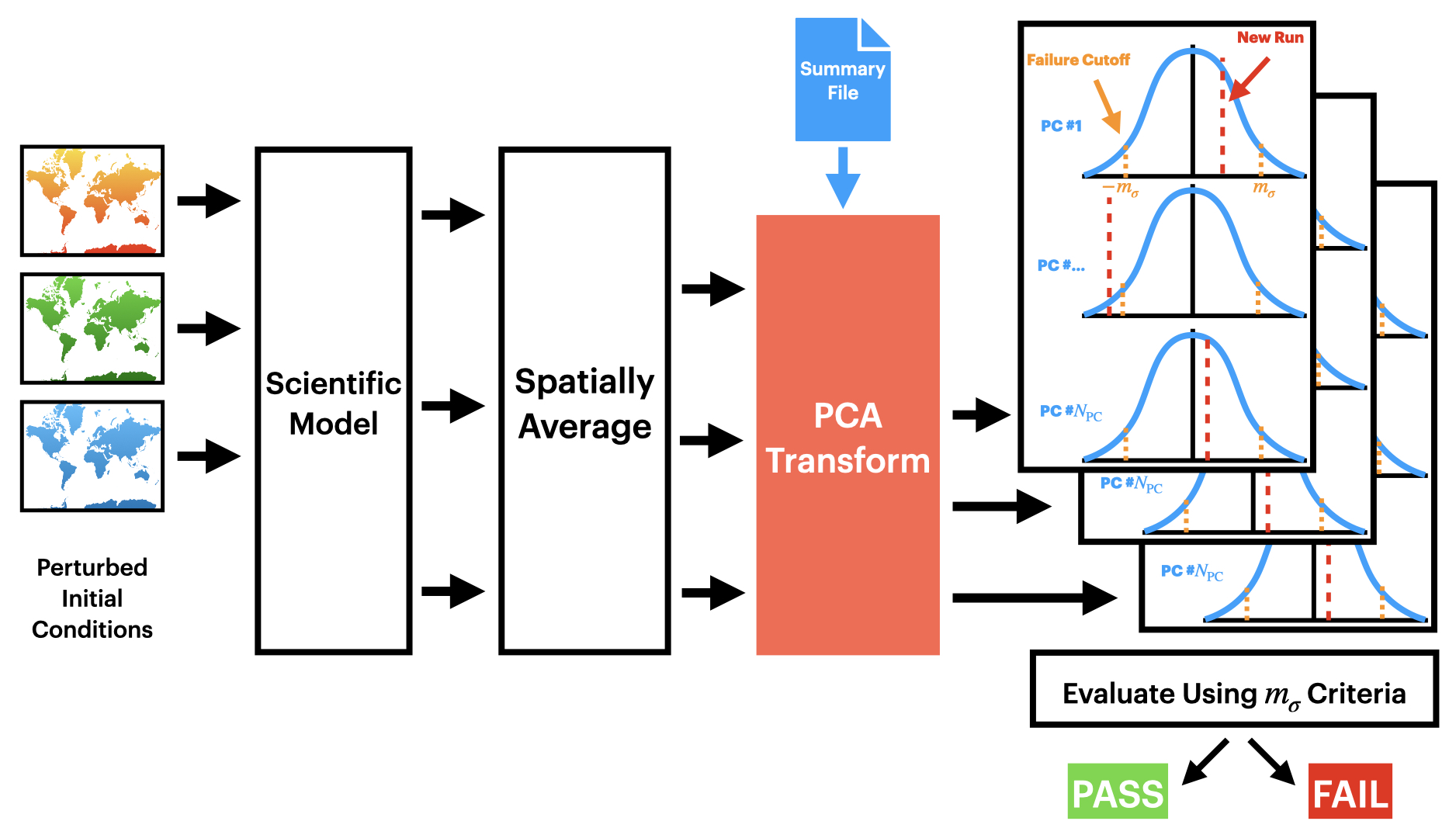
Figure 2 Diagram of the procedure for testing a new configuration with UF-ECT.

2.1 UF-ECT procedure

We now outline the UF-ECT procedure. This procedure is implemented as part of the previously mentioned PyCECT software library.

• 1.

  Generate an ensemble of N_ens numerical model runs from the reference configuration.

  • -

    In the PyCECT implementation, ensembles are generated by perturbing a field of the initial conditions by machine-level perturbations and running the model forward for time T. There may be other ways to generate an ensemble that captures the internal variability of the model to be tested but perturbations to the temperature field are the most common for CESM ensembles. The final instantaneous state of the model at time T is considered the output.

• 2.

  Exclude variables.

  • -

    Before characterizing the ensemble, variables with zero or very small variance, linearly correlated variables, and noncontinuous variables (such as integer valued outputs) are excluded to avoid numerical issues associated with low-rank or non-invertible matrices.

• 3.

  Spatially average variables.

  • -

    If the numerical model output includes spatial variables, those spatial output variables are averaged down to a single scalar. This averaging may look slightly different depending on the variable and model. Generally a weighted averaging scheme is used if outputs are defined on cells with different sizes.

• 4.

  Characterize the ensemble using principal component analysis (PCA).

  • -

    Before calculating the PCA transformation, variables are standardized, resulting in zero mean and a standard deviation of 1. This step is important in settings where variables may be measured on very different scales, common in scientific models. The associated shifts and scales are saved for equivalently transforming the output from the new configuration to be tested.

  • -

    This step will result in a set of PCA loadings, the vectors used to transform from the model's output space to the PCA space, and standard deviations (σ) for each principal component (PC), an estimate of the underlying variance of that PC. Each PC has a mean of zero by construction.

  • -

    Retain the first N_PC loadings and σ values that explain most of the variance of the model output.

• 5.

  Generate N_new model runs from the test model configuration, then transform the output variables using the PCA loadings (Fig. 2).

  • -

    N_new=3 is considered fixed for this paper.

• 6.

  Determine a failure or pass using the following steps.

  • -

    Categorize each PC of each new test run as a failure if it lies more than m_σ standard deviations away from the mean. For example, if m_σ=1.0, then a particular PC will be categorized as a failure if it falls more than 1.0 standard deviation a way from the mean of the reference ensemble. In this way m_σ defines the width of the test's acceptance region.

  • -

    The overall ECT results in a failure if N_pcFails PC components fail N_runFails or more of the new test runs.

  • -

    m_σ is chosen in order to achieve a desired FPR. N_pcFails=3 and N_runFails=2 are considered fixed for this paper.

2.2 PCA estimation bias

Because the failure of a particular PC from a test model run depends on where it lies within the distribution estimated from the reference ensemble, effective estimation of that distribution is key to the ECT method. Unsurprisingly, the accuracy of estimating the underlying distribution improves with more samples (i.e., a larger ensemble). However, PCA estimation error does not affect each PC randomly. Instead it follows a structure described in Lawley (1956) and Jackson and Jackson (1991), where, with ensemble size n and true PC variance λ_i, the expected value of estimated variance l_i is

$$\begin{array}{}\text{(1)}& E\left(l_i\right)={\mathit{\lambda }}_i\left[\mathrm{1}+{\displaystyle \frac{\mathrm{1}}{n}}\sum _{j\ne i}^p\left({\displaystyle \frac{{\mathit{\lambda }}_j}{{\mathit{\lambda }}_i-{\mathit{\lambda }}_j}}\right)\right]+O(\mathrm{1}/n^{\mathrm{2}}).\end{array}$$

As stated in Jackson and Jackson (1991), “the general effect is that the larger roots will be too large and the smaller roots will be too small,” where roots refer to the variance of a particular PC dimension (Fig. 3). This effect decreases as ensemble size grows and also depends on the relative size of the true variances.

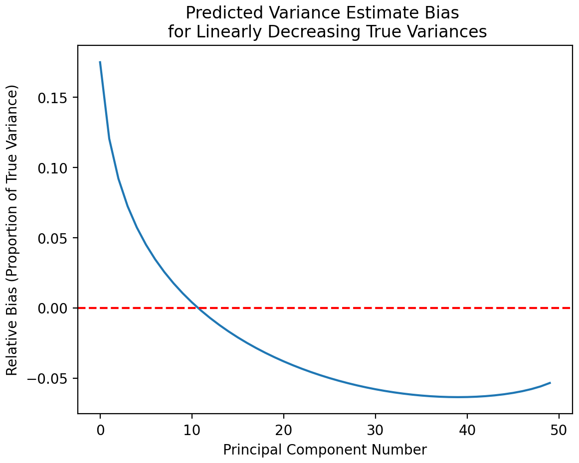
Figure 3 Theoretically predicted variance of a system with linearly decreasing true PC variances. The system contains 50 dimensions and 1000 samples. We see a region where early (i.e., larger) PC variances are overestimated (positive bias) and a region where later (smaller) PC variances are underestimated (negative bias). This bias affects the UF-ECT in multiple ways.

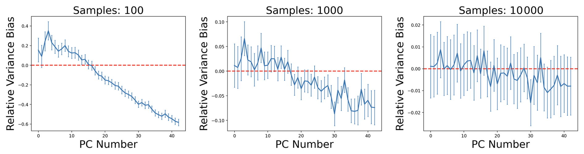
Figure 4 PCA variance estimation bias observed when randomly generating samples from a multivariate Gaussian distribution created to emulate the structure of scientific model outputs. One can see the clear impact of increasing the number of samples (also known as ensemble members) with sample size growing left to right. While the overall structure of bias predicted by Eq. (1) can be seen, it is neither smooth nor predictable. This makes accounting for the bias without increasing the ensemble size difficult.

Figure 5 True PC distributions are in blue and estimated PC distributions are in red. Vertical lines represent true and estimated m_σ. If the estimate of a PC variance is overestimated (as in a) the ECT will miss failures that occur in the blue region. Alternatively, if the estimate of variance is underestimated (as in b) the ECT will return additional false positive failures in the red region. Importantly, the effects of different directions of PC bias (as in Fig. 4) do not cancel each other out.

This bias affects the ECT in multiple ways. For PCs whose variance is overestimated, a new test run is less likely to fail than if the variance were perfectly known. This is because the region of acceptance is increased as the estimated σ grows. In contrast, for PCs whose variance is underestimated, new test samples that should not fail instead fail more often than they would with perfect knowledge of the variance. This occurs because the region of acceptance is reduced as the estimated σ shrinks (see Fig. 5). A key note is that the effects of overestimated and underestimated PCs do not cancel each other out. Instead, a poorly estimated PCA transform could result in both additional missed true failures and false positives. Finally, this bias can impact one's estimate of how many PC dimensions are needed to capture the underlying dimensionality of the numerical model.

If the bias was smooth and predictable it would be easy to account for. Unfortunately, the interplay of stochastic noise and the bias terms results in a highly noisy bias (as shown in Fig. 4). The impact of bias on the ECT was explored in previous work (Molinari et al., 2018) and alternative estimators were tested. Alternative estimators were found to reduce bias on average but introduce unacceptable uncertainty to the estimates of PC variance. In this current work, conscious of these effects, our goal will be to generate a sufficiently large ensemble and specify the number of PCs used to manage the effects of the bias.

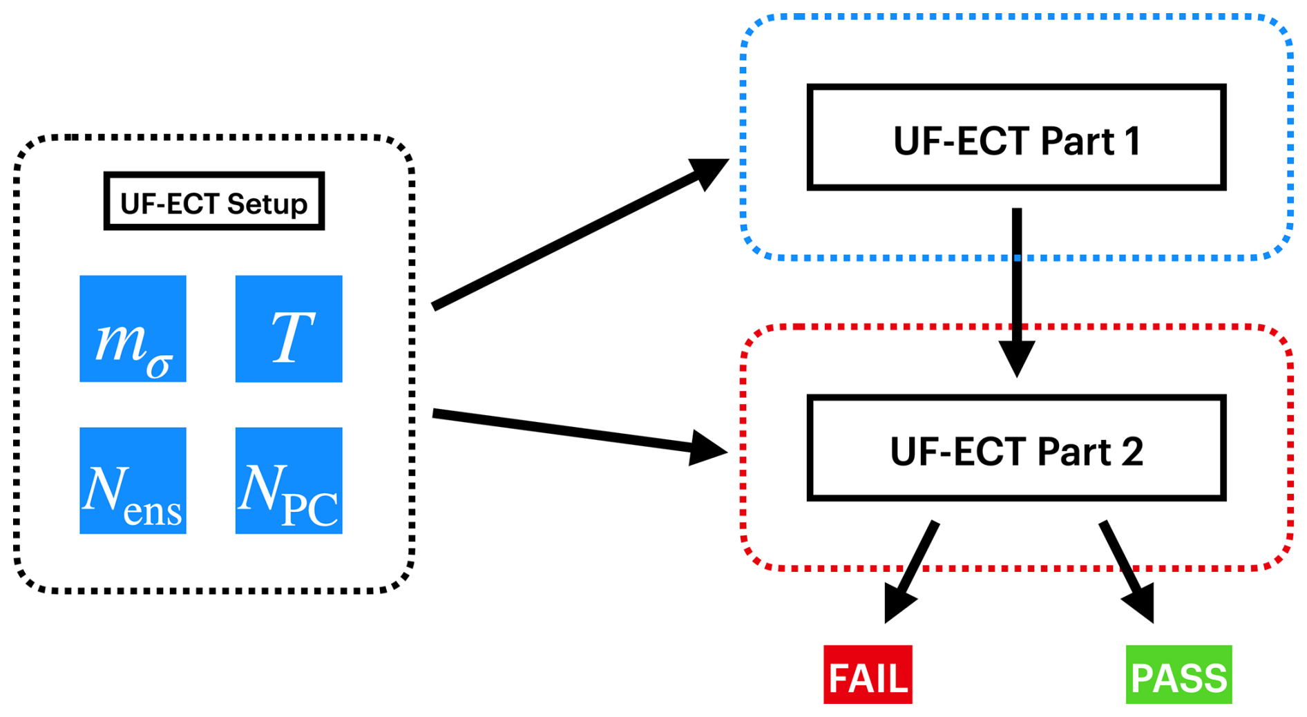
Figure 6 When applying the UF-ECT to a different model, developers must first undertake certain setup steps to appropriately specify test parameters that reflect the size and behavior of their model. These test parameters affect all parts of the test, from generating the large reference ensemble and characterizing it using PCA (part 1) to running and evaluating runs from the new test configuration (part 2).

3 A generalized setup framework for applying the UF-ECT to different computer models

In this work we develop a general setup framework for applying the UF-ECT to different models and specifying the values of relevant test parameters. One can think of this work as a setup phase (Fig. 6) of the test, which model developers must undertake when first adapting the UF-ECT procedure to their application. This work only has to be done once for a given numerical model or when an existing model undergoes substantial scope changes, such as adding significant new science. (If users, for instance, want to designate a new computing cluster as the source of their accepted configuration, this setup phase will not have to be redone.)

Because of the interaction of various test parameters, we propose the following ordering when specifying parameters to use the UF-ECT method on a new or updated model. Exactly how to specify these parameters is explained in the following section.

1. Generate a sufficiently large experimental ensemble for the setup phase.

2. Determine an appropriate model run length, T.

3. Determine which output variables to exclude from the test.

4. Determine the number of PC dimensions to use in the test, N_PC.

5. Determine the width of the acceptance region, m_σ, and reference ensemble size, N_ens.

3.1 Generating an experimental ensemble

The first step to specifying appropriate UF-ECT parameters involves the generation of a large experimental ensemble of numerical model runs. These runs are generated in the same way as they would be for the test itself, with two important differences. First, the number of ensemble members is higher than it will be for the eventual summary file creation in part 1 of UF-ECT (see Sect. 2.1). This allows us to test a range of parameter values and ensemble sizes (and multiple permutations of each ensemble size) to be confident in our parameter specifications. Second, because we do not yet know how long the model must be run for, we must save multiple time slices of the model and use longer runs than will eventually be required.

Both of these requirements result in increased computation and storage costs. However, it is important to remember that even if models are run for twice as long and the ensemble is twice as large as required in part 1, the cost will still be reasonable because of the length of the ultrashort runs. In addition, if storage of multiple time slices is an issue, one can reasonably save every nth time step without substantially impacting one's conclusions.

Based on our experience with the numerical models in this paper, we recommend beginning the setup phase with an experimental ensemble size (N_exp) equal to 10 times the number of output variables of the model, after known constant and non-floating-point variables are excluded (again, this large experimental ensemble is used only for the setup framework and will be used to specify needed UF-ECT parameters, including N_ens). This size is a heuristic based on our experience. Having a larger experimental ensemble than necessary will not negatively impact our results. Also, in a subsequent step we will be able to determine if the heuristic recommendation is too small and generate additional runs for a larger experimental ensemble.

To demonstrate our generalized setup framework we will include results using MPAS-A (Skamarock et al., 2012). For all MPAS-A results we use version 7.3. MPAS-A uses a C-grid staggered Voronoi mesh, and our work uses a quasi-uniform 120 km mesh with 55 vertical levels and 40 962 cells. The default output files from MPAS v7.3 contain over 100 variables. However, a number of these variables are actually constant over time (e.g., the area of each grid cell) or are purely diagnostic, in the sense that they are computed from the model prognosed state but in no way influence the simulation. Eliminating constant variables and diagnostic variables left 43 variables in the model output, and hence we begin with a recommended experimental ensemble size of N_exp=430. In general, determining the appropriate set of output variables is best done by or in conjunction with model developers.

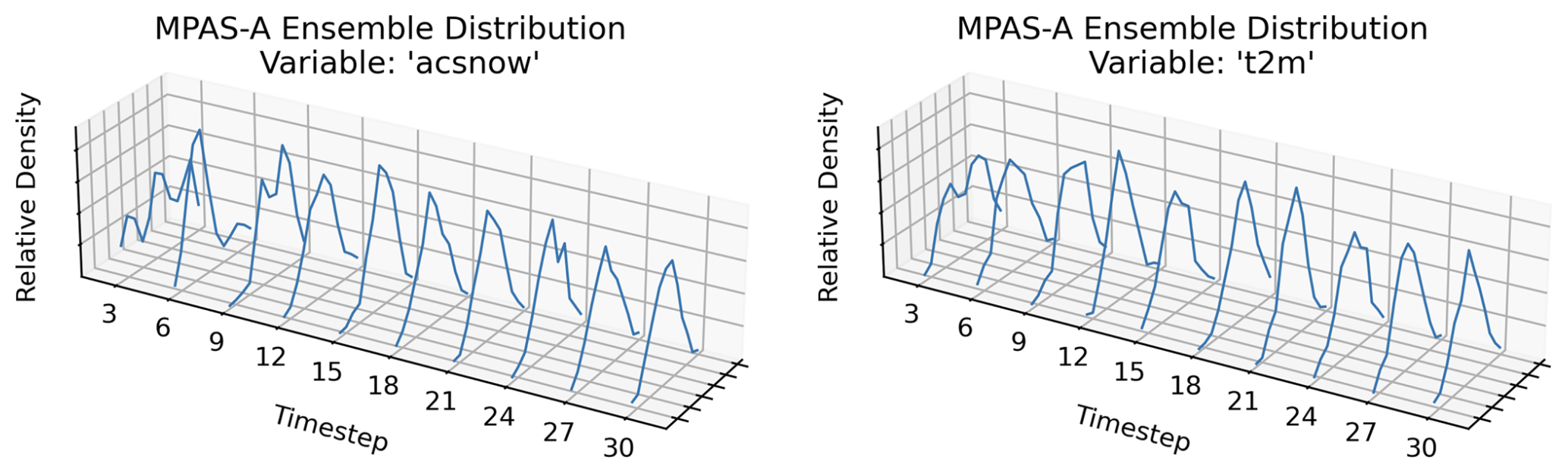
Figure 7 Plots demonstrating the evolution of an experimental ensemble of spatially averaged outputs from MPAS-A. The distributions of both variables (with acsnow representing accumulated snow and t2m representing temperature at 2 m height) look roughly normal after 12 time steps of the model (approximately 2.5 h of simulated time). However, t2m looks roughly normal earlier, perhaps reflecting closer coupling to the original perturbations.

3.2 Determining an appropriate model time slice

The UF-ECT method relies on effectively quantifying the underlying variable distributions of each numerical model. For this purpose we seek to run the model long enough that we can effectively detect the impact of model changes in model outputs. Running too long will lead to excess computational expense or, worse, having the output signal totally dominated by chaotic effects as model trajectories diverge according to the Lyapunov exponents of the system. Initially, and for the first few time slices, the spatial average of most variables will not be normally distributed across the experimental ensemble, as only a single variable field was perturbed. As the ensemble is allowed to run for longer, the ensemble distribution of each variable will generally spread out (see Fig. 7) until they reach the limits of the model's underlying phase space.

This behavior is directly related to our reliance on the central limit theorem to approximate the spatial means of numerical model outputs and their PCA transformations as normal distributions. The assumption of variable outputs as random fields is only valid if the model has been run long enough where each variable's output can be treated as a stochastic process despite only perturbing one variable's initial conditions.

As the perturbations of one variable field propagate through the numerical model, the number of variable distributions failing a test of normality quickly decreases before stabilizing. We have found this transition to normality to be a useful way to determine when a model has been run long enough to be used for the UF-ECT. One measure of normality is the Shapiro–Wilk test (Shapiro and Wilk, 1965). An in-depth discussion of the Shapiro–Wilk test as applied to CESM can be found in Molinari et al. (2018). In Fig. 8 we see a plot of how many variables fail the Shapiro–Wilk test (with the commonly used p=0.05 cutoff). One can see that the number of variables failing the normality test falls from an initial peak and then stabilizes around a lower number, though usually not zero. For MPAS-A, this transition appears to take place after approximately 12 model time steps (using the default time step length of 12 min), so we set T=12 time steps. If the number of variables failing the Shapiro–Wilk test does not decrease and then stabilize, a user should be concerned that their model is not behaving like those we investigated and perhaps the initial perturbations are not propagating across fields. Since the Shapiro–Wilk test is probabilistic, this number would not go strictly to zero even if all the variables were sampled from normal distributions. In reality variable distributions are unlikely to all be strictly normal. We will revisit that possible issue in the next section.

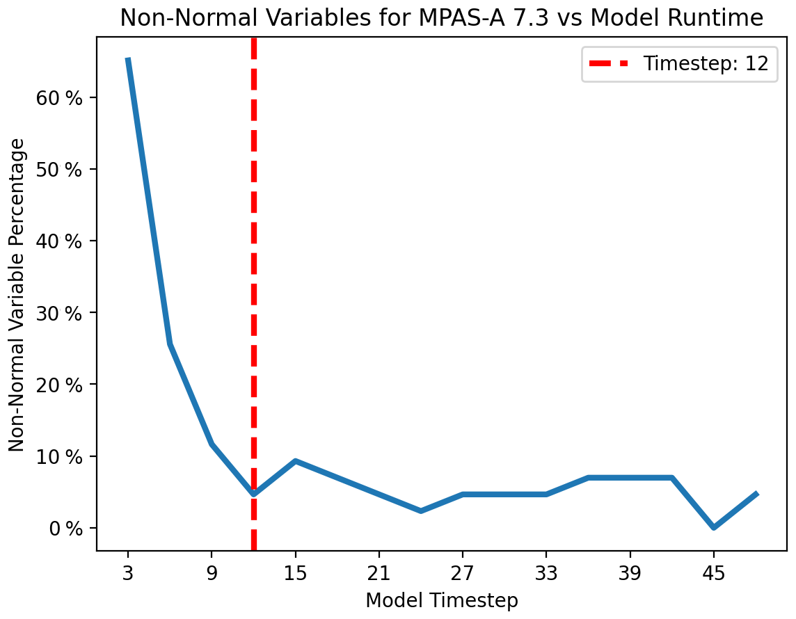
Figure 8 Number of MPAS-A output variables failing the Shapiro–Wilk normality test (considered a p value < 0.05) as a function of model run length. One can see the number of non-normal variables decreasing before stabilizing. This transition is used to specify an appropriate length to run the model (T). The dashed red line is placed at time step 12.

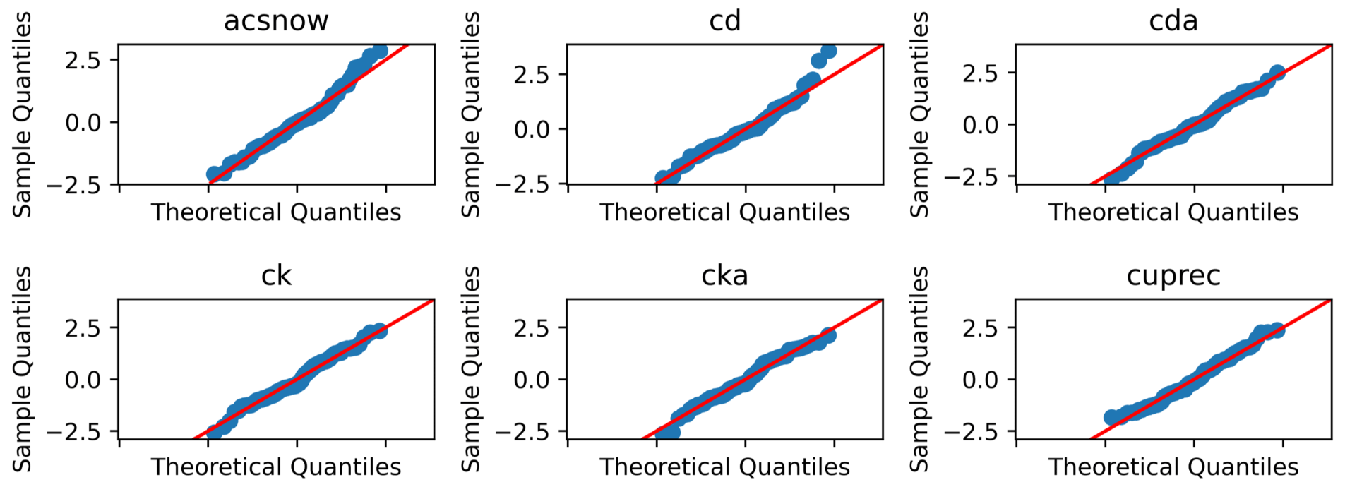
Figure 9 Selection of MPAS-A Q–Q plots. Samples falling along the diagonal red line indicate that the distribution matches a theoretical normal distribution. Variable descriptions are as follows – acsnow: accumulated snow, cd: drag coefficient at 10 m, cda: drag coefficient at lowest model level, ck: enthalpy exchange coeff at 10 m, cka: enthalpy exchange coefficient at lowest model level, and cuprec: convective precipitation rate.

In some numerical models, default initial conditions may not be representative of a fully spun-up model state, where fields are in balance and contain structure commensurate with the model grid resolution. In these cases it is possible that the UF-ECT, and the setup framework developed here, should use an initial state generated after some amount of spin-up. MPAS-A developers indicated that hydrometeor fields require some model spin-up, so all MPAS-A results begin from a state generated from a 1 d spin-up simulation. No significant difference was observed in the amount of time required for the count of non-normal variables to stabilize. But, as the incurred computational cost from a single spin-up run is small, if model developers believe default initial conditions are unrealistic we recommend using a post-spin-up set of initial conditions for creating the ensemble.

Another way to analyze the normality of variables is using Q–Q plots like in Fig. 9. These plots visualize whether the density quantiles of the ensemble match those of a theoretical normal distribution. All ensemble members (blue markers) falling on the red line would indicate matching a normal distribution. We found visual inspection of Q–Q plots to generally agree with conclusions drawn from the Shapiro–Wilk test. However, as each variable generates a plot at each time slice, this approach can become unwieldy for any substantial number of variables. Therefore, they are not recommended as part of the generalized setup framework for specifying the time slice to use for UF-ECT but could be a helpful tool if a user of the framework is running into oddities.

3.3 Determining which variables to exclude from the test

Large scientific numerical models may output a variety of variables by default, some of which should first be excluded before using the UF-ECT. Generally this is because some variables do not carry unique information and/or may introduce numerical issues in later steps. While model users may already be able to identify many such variables (for instance a variable used to describe the grid whose value does not change over time), we now consider such variable categories and their impact on UF-ECT performance.

Variables that are constant, or very nearly constant in a numerical sense, across the ensemble are the first to be excluded. Such variables introduce numerical issues when introduced to the PCA algorithm. As they do not help us characterize the ensemble, excluding them does not cause a loss in sensitivity of the test. Because the test relies on quantifying and comparing to continuous distributions, discrete outputs are excluded. Model developers should be careful if their model's output is largely integers or other non-floating-point variables. Both of these classes of variables are already excluded as part of the PyCECT software.

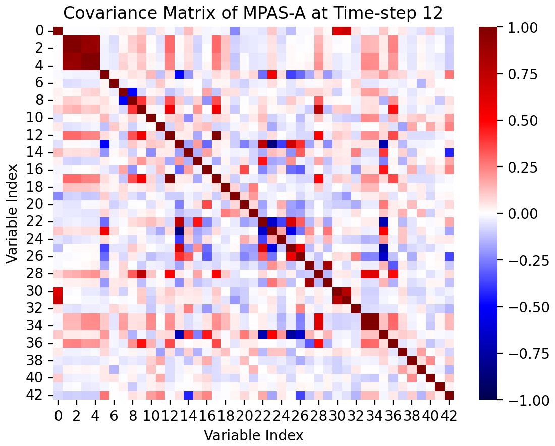
Figure 10 Correlation plot of MPAS-A output variables at time step 12. Relationships between highly correlated variables can be seen in dark red and dark blue.

Correlated variables can be common in scientific models. For example, temperature, potential temperature, and temperature at 10 m are all output by MPAS-A. Variables that are almost exactly linearly correlated, and thus result in a rank-deficient covariance matrix, are already excluded as part of the PyCECT software (using a QR-factorization approach with a tolerance based on machine epsilon and degrees of freedom) because they have the potential to introduce numerical issues. Further, due to being almost exactly linearly correlated, they will not help us better characterize the model. However, other variables still have a range of correlation intensity. A plot of correlation coefficients for MPAS-A can be seen in Fig. 10. From the 43 MPAS-A variables considered there were 13 variable pairs considered highly correlated. For this analysis we investigate variables having greater than a 0.75 correlation coefficient but not resulting in a rank-deficient correlation matrix as identified using the QR factorization described above.

Does including variable pairs with correlation coefficients in this range, not enough to cause numerical issues but far from being independent, negatively impact the UF-ECT method? Since all outputs will be transformed using PCA, we expect the correlated variables to be handled in that step. Indeed, dealing with correlated data is one of the main reasons for PCA. To test this assumption we ran a large set of UF-ECT simulations using a 430-member MPAS-A experimental ensemble.

These tests were done as follows.

1. Randomly select 200 members of the 430-member MPAS-A experimental ensemble.

2. Select a random set of three samples from the remaining members of the MPAS-A ensemble to serve as test members.

3. Record how often each individual PC from the test runs fell outside the m_σ acceptance region according to the standard ECT procedure.

4. Repeat steps 2 and 3 for 100 iterations.

5. Repeat steps 1–4 for 100 iterations.

This approach was used to calculate which PC dimensions contributed most to failures and, by transforming the failing PC dimensions back into the variable space, which model variables contributed most. As all these model runs were from the same model configuration, these failures are “false positives”. We see in Fig. 11 that the rate at which an individual PC dimension from a test run would fall outside the m_σ acceptance region steadily grows as the estimated variance of that PC dimension grows. This is a result of the PCA variance estimation bias discussed earlier.

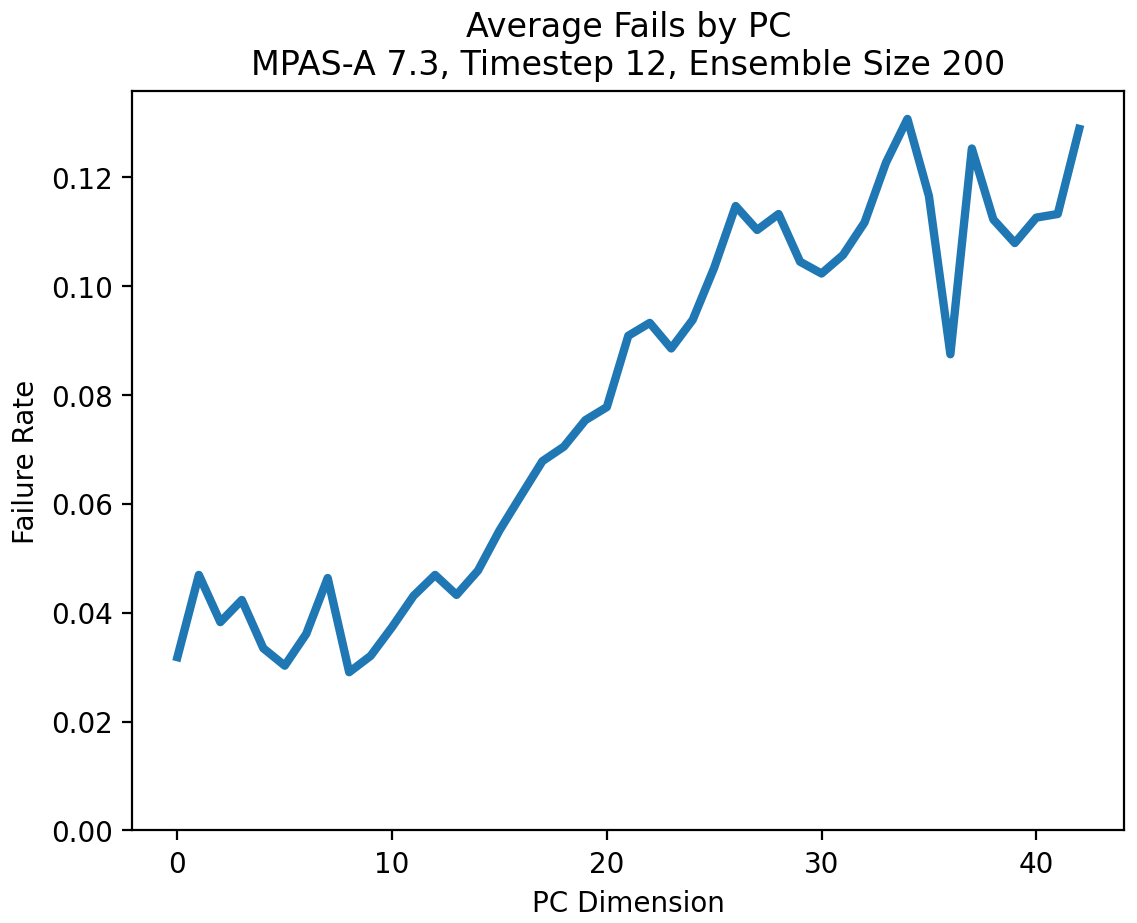
Figure 11 Average failure rate of each MPAS-A PC dimension based on samples from the same model configuration. Note that this failure rate is not the same as the overall UF-ECT FPR as it only signifies that a particular PC falls outside the acceptance region (this is why the failure rate is much higher than the expected UF-ECT FPR). The figure indicates that the later PC dimensions representing a smaller proportion of the ensemble's variance are more likely to fail due to bias in their estimate.

In Fig. 12 we see the average contribution to failure of each MPAS-A variable. The x axis is arbitrary and reflects the original ordering of the variables in their output files. One can see that the likelihood of contributing to a failing PC dimension is roughly equal across all included MPAS-A variables. It appears that no specific variables, including the correlated variables highlighted earlier, cause disproportionate rates of false positives.

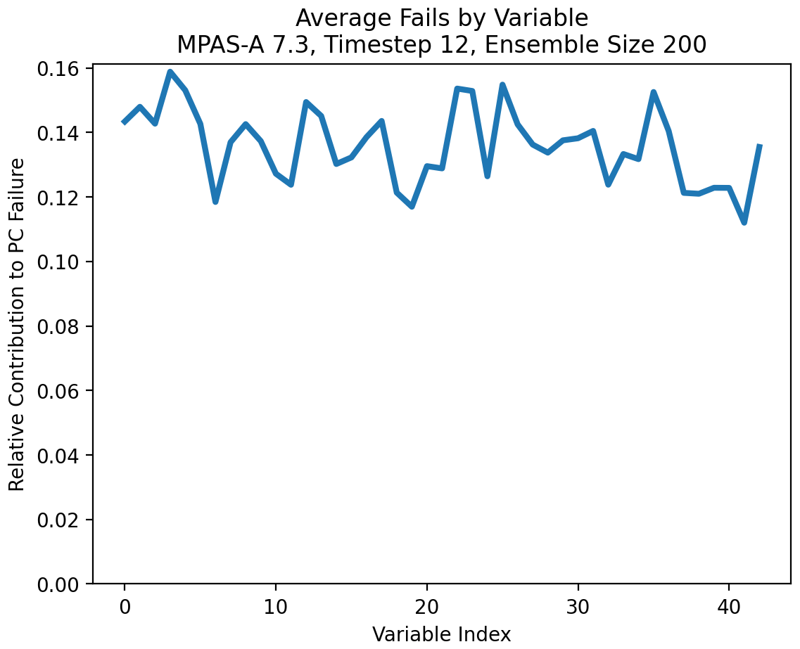
Figure 12 Result of transforming the failing PC dimensions from Fig. 11 back into the MPAS-A variable space. This figure shows the relative contribution of each model variable to failing PCs. Again these values do not equate to the overall UF-ECT FPR, but this figure shows that all variables contribute roughly equally to false positives. This gives us confidence that our setup framework has excluded numerically problematic variables.

This also gives us confidence that every spatially averaged variable distribution being strictly normal is not a requirement for the UF-ECT. When we specified a time slice, we waited until the number of variables whose distribution across the ensemble was non-normal stabilized (Fig. 8). But some variables may continue to fail the test for normality in later time slices (Fig. 7 gives an example of how variable distributions may look in later time slices). Again, Fig. 12 indicates that variables failing the normality test do not contribute disproportionately to false positives.

Based on these results we do not recommend additional exclusions beyond those historically excluded by the PyCECT software library based on numerical issues. These include variables that are constant, numerically close to being constant, non-floating-point, and linearly dependent (due to resulting rank-deficient covariance matrices). Therefore no new correlation calculations are required as part of the setup phase.

It is worth mentioning that we expect the existing procedure to adequately handle the case where a user has added additional derived variables or where it is difficult to distinguish which output variables are natively calculated versus derived.

3.4 Determining how many PC dimensions to use

PCA forms an important part of the UF-ECT method. Transforming the spatial means into an orthonormal basis allows us to compare to each PC dimension independently. Also, if the underlying dimensionality of our data is less than the number of output variables, PCA allows us to utilize a smaller number of dimensions. In this case we can ignore PC dimensions that do not capture information about the model.

But we do not want to miss an error because we discarded too many PCs, a result referred to as a false negative, and thus failed to capture information about part of the model. Including a sufficient number of PCs is key to achieving the goal of accurately characterizing the model. A common approach to determining how many PCs to use is to consider the cumulative variance explained of the first N PCs. We will adopt this approach to specify a sufficient number of PC dimensions using a standard of explaining 95 % of the ensemble's variance. While not used in this approach, it is worth noting that numerous methods of determining the appropriate N_PC exist as described in Cheng et al. (1995), Richman and Lamb (1985), and North et al. (1982). While variance explained has proven sufficient for our current method, an alternative method may be explored in future work.

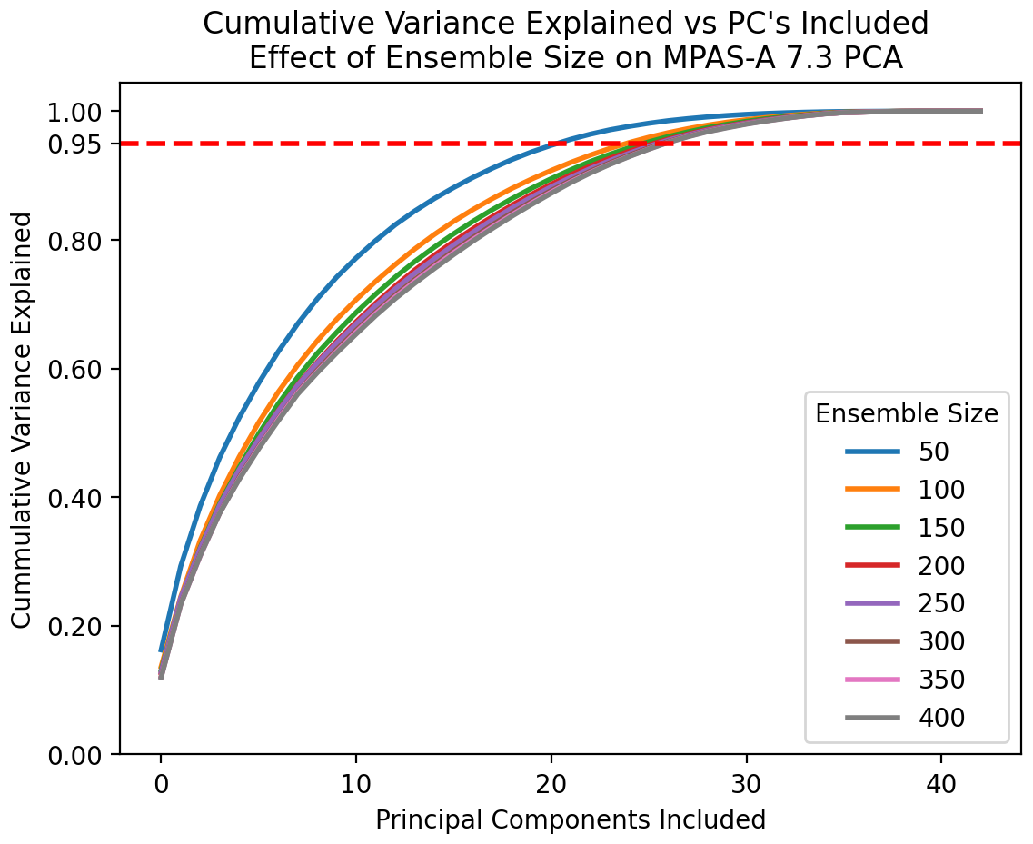
Figure 13 Estimated cumulative variance of a given number of PC dimensions for MPAS at various sample sizes. One can see that small sample sizes underestimate the number of PCs required to explain a given amount of variance. Figure reflects the mean of 10 sets of samples at each ensemble size.

However, another side effect of the PCA bias discussed earlier is that using an insufficient ensemble size causes one to underestimate the number of PCs required to explain a given amount of variance. With a small ensemble size, the variance of the early (larger) PCs is overestimated. This effect is seen in Fig. 13. As the ensemble size used to estimate the PCA transform grows, the curves converge to a stable estimate.

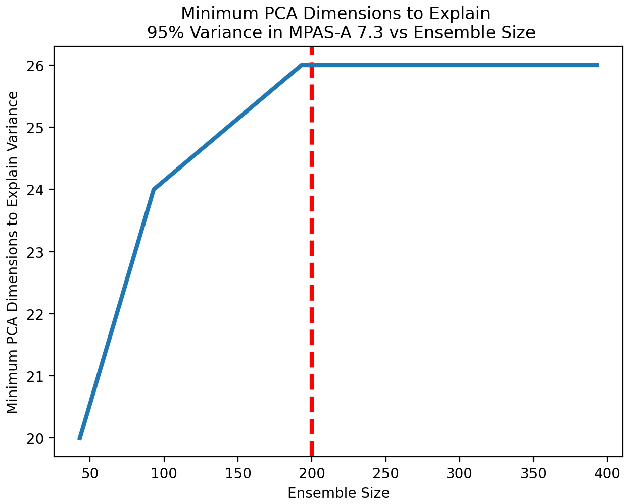
Figure 14 Estimated number of PC dimensions required to explain 95 % of the variance in MPAS as a function of ensemble size. This number rises as the effect of bias is reduced, eventually stabilizing to 26 PC dimensions after an ensemble size of 200 members. The figure reflects the mean of 10 trials at each ensemble size.

For the UF-ECT setup phase, our goal is to include enough PC dimensions to explain 95 % of the variance of the numerical model. We can see that our required PC dimensions needed to explain 95 % of the variance stabilize beyond a sufficient ensemble size (Fig. 14). We consider the required PC dimensions to have stabilized when their value stays constant over a 250-sample-size increase (in steps of 50 samples). We will use this stabilized count for N_PC. In addition, this provides a minimum ensemble size (N_ens) to use. If our estimate of N_PC does not stabilize with an ensemble size smaller than our experimental size, with a sufficient margin to conduct repeated trials, we know we must create a larger experimental ensemble. In this way we are able to adjust our original experimental ensemble size heuristic as needed.

Based on this process, we recommend N_PC=26 for UF-ECT when used with MPAS-A.

3.5 Determining an appropriate acceptance region and ensemble size

We have now determined the time span to run the numerical model, the number of PCs, and the ensemble size that gives us a stable estimate of overall model variance. These steps address the important task of ensuring that we are sensitive to changes across a scientific model code, as long as all portions of the code are represented in the output variables.

We must also ensure that the number of false positive results remains below an acceptably low rate, where model configurations that should pass are issued failures. Too many false positives reduce the practical usefulness of the UF-ECT, but some false positive results are an intrinsic effect of the probabilistic nature of the UF-ECT. Even results from the original model's distribution of outputs will sometimes fall outside the acceptance region defined by m_σ. The likelihood of failing the test, holding other test parameters fixed, goes up as we increase N_PC, just as the odds of rolling double ones on a pair of dice go up when given more attempts.

For a given value of m_σ, we can derive the theoretical FPR as a function of N_PC, assuming distributions are perfectly Gaussian and we have exact knowledge of each distribution's variance. When m_σ=2.0, as it has been the default in previous works, the probability of an individual PC failing a specific run is equivalent to the likelihood of a Gaussian variable falling more than 2 standard deviations from the mean or

$$\begin{array}{}\text{(2)}& {\displaystyle }& {\displaystyle }{m}_{\mathit{\sigma }}=\mathrm{2.0},\text{(3)}& {\displaystyle }& {\displaystyle }r=\mathrm{2}\cdot \mathrm{\Phi }(-m_{\mathit{\sigma }})=\mathrm{0.0455},\end{array}$$

where Φ(x) represents the cumulative distribution function of the standard normal distribution. The constant value of 2 is a result of considering values both sufficiently less than and more than the mean. The probability of a specific PC failing two or more runs out of three can be derived from the cumulative distribution function of the binomial distribution. It is equivalent to asking the following question: given three trials, what is the likelihood of two or more successes when the probability of one success is r? It can be calculated as

$$\begin{array}{}\text{(4)}& p=\mathrm{3}{r}^{\mathrm{2}}(\mathrm{1}-r)+r^{\mathrm{3}}=\mathrm{0.006}.\end{array}$$

Finally we can calculate the probability of N_pcFails=3 or more failures when using N_PC PCs using the same cumulative distribution of the binomial distribution but where each trial's chance of success is now p. The equation is simplified if we subtract the probability of failing two or fewer PC dimensions (results that would actually result in a test pass) from one to give us our failure rate:

$$\begin{array}{}\text{(5)}& \mathrm{FPR}\left(N_{\text{PC}}\right)=\mathrm{1}-\sum _{k=\mathrm{0}}^{\mathrm{2}}\left(\genfrac{}{}{0ex}{}{N_{\text{PC}}}{k}\right)p^k(\mathrm{1}-p{)}^{N_{\text{PC}}-k}.\end{array}$$

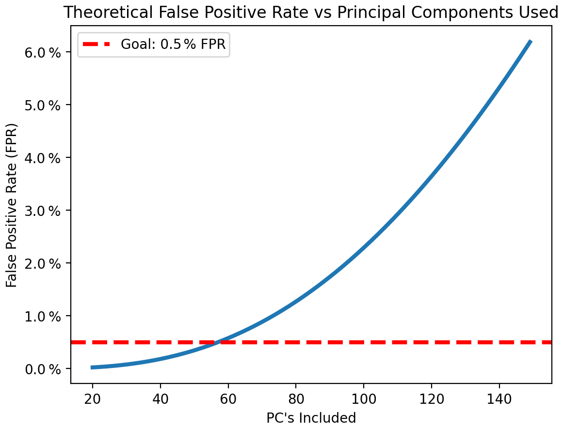
Figure 15 Theoretical FPR of the UF-ECT as a function of N_PC if PC distributions were Gaussian and their variance was perfectly known when m_σ=2.0.

Plotting this function for a range of N_PC we see that, when using 26 PC dimensions as we chose for MPAS-A, the theoretical FPR falls below our goal of 0.5 % (Fig. 15). If this was not the case, as we will see later when examining CESM, we can adjust m_σ. For MPAS-A, we continue to use the default m_σ=2.0 (extensive discussion of the ECT FPR and a derivation of the theoretical FPR can be found in Molinari et al., 2024).

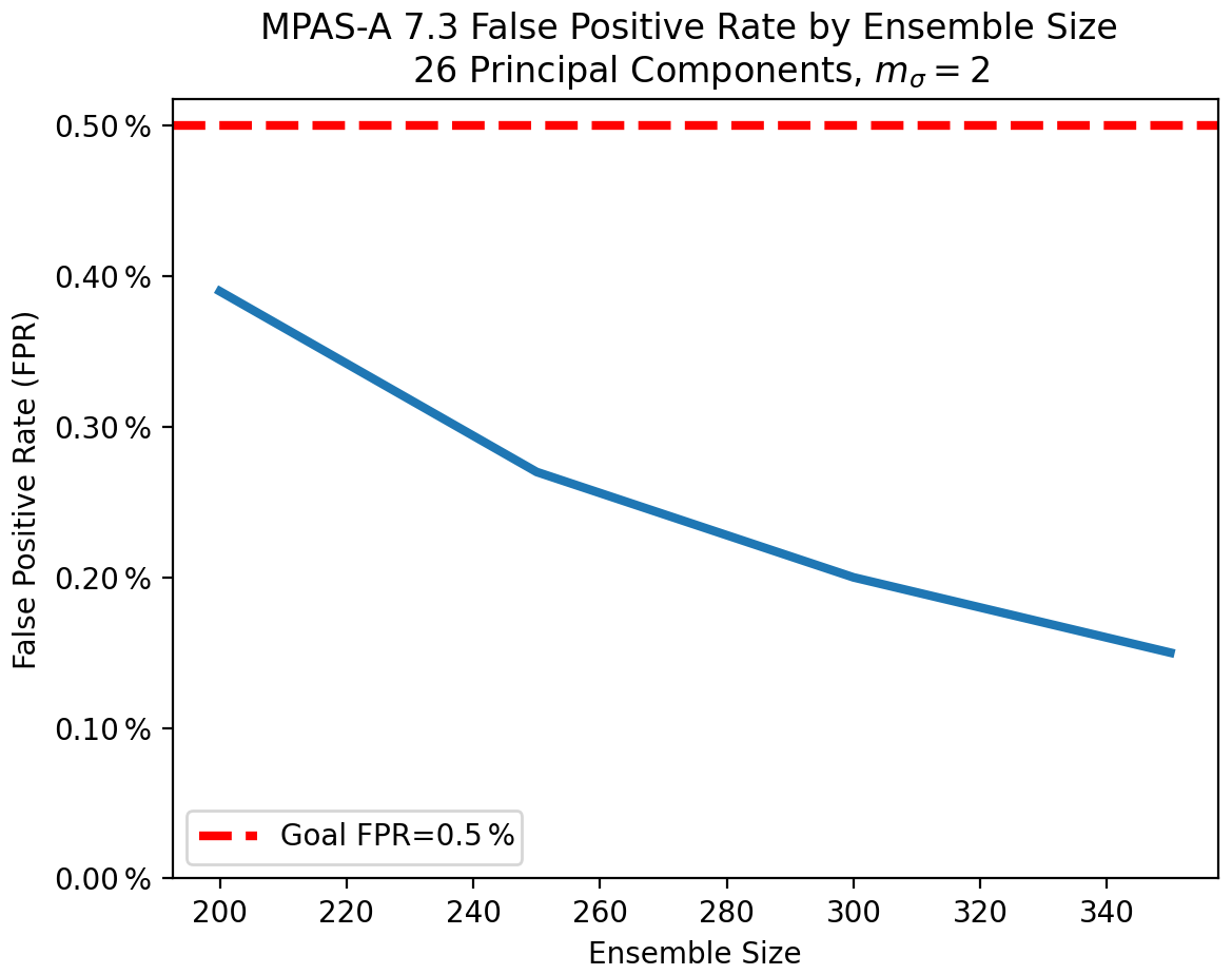
Figure 16 Experimental FPR for the UF-ECT when used with MPAS and N_PC=26. The plot represents a mean of 10 000 trials at each ensemble size.

However, just because we can theoretically achieve a FPR below 0.5 % does not mean this occurs in practice. The PCA bias discussed earlier, as well as deviations from normality, can cause additional false positives. These effects are reduced as we increase our ensemble size (an in-depth exploration of the effect of ensemble size on FPR can be found in Molinari et al., 2018). By repeatedly running the UF-ECT using subsets of our larger initial experimental ensemble and testing remaining runs we can estimate the actual FPR for a model at a given ensemble size (Fig. 16). We see that an FPR less than 0.5 % is achieved at the ensemble size of 200 that yielded stable variance explained estimates in the last step. Therefore for MPAS-A we recommend N_ens=200.

These last two steps, determining N_PC and N_ens, inform our recommendation to initially generate a larger experimental ensemble of runs for the setup framework. In order to be confident that our ensemble size estimates are valid we need a substantially larger experimental ensemble to draw from.

We have now estimated all needed UF-ECT test parameters. For MPAS-A these were T=12 time steps, N_PC=26, m_σ=2, and N_ens=200. In Sect. 5, we will test the effectiveness of these parameter choices.

4 Re-evaluating the UF-ECT for CESM 2.3

In the previous section we detailed a setup framework to determine appropriate parameters for the UF-ECT when applying it to a different model. Here we consider a slightly different task but for which we can apply the same approach. UF-ECT has been in use during CESM development for a number of years (again, we use the term CESM here, though we only focus on outputs from the atmospheric portion of the model, CAM). Indeed, UF-ECT was designed specifically for use with CESM and, as such, parameters like m_σ and N_PC were tailored to the model. However, in the intervening years CESM has gone through substantial development. Importantly for our purposes here, the model has grown to encompass new physics processes, reflected in a substantial increase in default output variables (after excluding variables as described above the model has gone from 108 default variables in the CESM version 1.3 series to 275 default variables in the version 2.3 release series). It is possible that some of the variables reflect simple transforms of existing variables. But, CESM developers are justifiably concerned that the UF-ECT parameters initially determined are no longer appropriate.

We begin our process as before, with the creation of an experimental ensemble 10 times larger than the default output size. With 275 output variables (after exclusions as outlined in Sect. 3.3) this results in an experimental ensemble of N_exp=2750 perturbed model runs. For the following analysis, we use the CESM 2.3 series release with the F2000climo compset and the f19_f19 resolution, which corresponds to a roughly 2° resolution on a finite-volume grid (we will refer to this resolution as “2-degree” for convenience). The CAM component is version 6.3.

Finally we will consider this important question: can we expect test parameters calculated for one model resolution to hold for other resolutions? To answer this question we will repeat our setup framework with CESM 2.3 but run using the f09_f09 resolution, corresponding to approximately a 1° resolution.

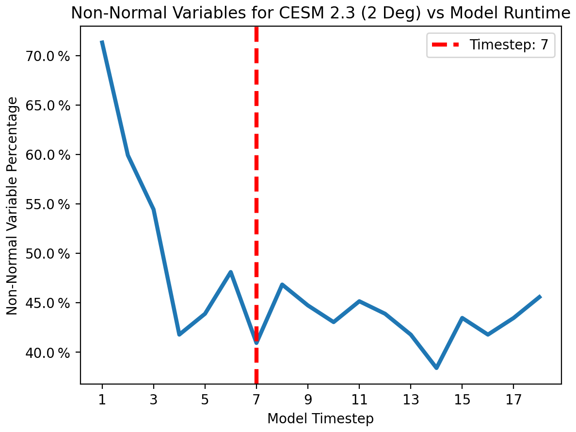
Figure 17 Non-normal variables (those with Shapiro–Wilk p score < 0.05) compared to model run length. In order to compare across all run lengths, variables that are not calculated at every time step are excluded. While this trend is noisier than with MPAS-A above, we see a clear trend. We identify seven time steps (marked with a vertical red line) as the point at which the quantity of non-normal variables stabilizes.

4.1 Determining an appropriate run length

With a sufficiently large experimental ensemble, the second step when applying UF-ECT to CESM 2.3 is to determine an appropriate model run length. Again, this is done by identifying the point at which the number of non-normal variables stabilizes. This transition represents the point at which the initial temperature perturbations have propagated to most other model variables and enables us to employ the central limit theorem. In Fig. 17 we can see that this occurs after just seven time steps. Identifying this transition is slightly more difficult than with MPAS-A above due to more noise in the results. Given the low additional cost of going from five to seven time steps, the slightly longer run length is selected to ensure that perturbations have fully propagated through the model. This length is roughly aligned with the previous use of nine time steps in Milroy et al. (2018). Some model variables in CAM are only calculated on odd time steps, and thus we only consider odd time steps to be viable candidates. Based on this process, we set the first test parameter: T=7 time steps.

4.2 Determining how many PC dimensions to use

With a run length specified we can now determine how many PC dimensions to use. Again, we seek to capture the bulk of the variability in our ensemble (and thus capture most of the behavior of the numerical model in question). But, due to PCA estimation bias, we will underestimate the number of PC dimensions required if we use an ensemble that is too small. By increasing our ensemble size until the required number of dimensions stabilizes we can be confident that we are fully representing the model.

Figure 18 Number of PC dimensions needed to explain 95 % of the variance in CESM 2.3 at time step 7 compared with sample size. The number of PCs required stabilizes at 130 beyond an ensemble size of 1450. The reported value represents a 10-trial mean.

In Fig. 18, we see that 130 PC dimensions are required to capture 95 % of the ensemble's variance. This estimate stabilizes beyond a sample size of roughly 1450. So, N_PC=130 for CESM 2.3.

4.3 Determining an appropriate acceptance region and ensemble size

Our final step to prepare the UF-ECT for use with CESM 2.3 is to ensure that our FPR is not too high, causing users to have to deal with too many erroneous false positives that do not actually correspond to meaningfully distinct outputs. The FPR is affected by PCA estimation bias but also increases as the number of PC dimensions increases as an unavoidable by-product of the test design. In Fig. 15 we saw the theoretical limit for FPR if we could perfectly estimate the underlying PC distributions. When 130 PCs are included in Fig. 15 we see that the theoretical FPR is well above our goal FPR of 0.5 %.

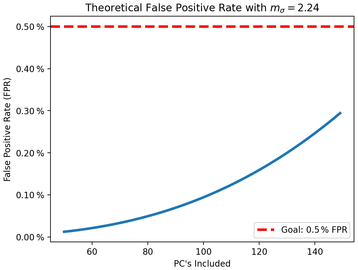
Figure 19 Theoretical FPR of the UF-ECT as a function of N_PC if PC distributions were Gaussian and their variance was perfectly known when m_σ=2.24.

By adjusting m_σ we can tune the sensitivity of the UF-ECT. Figure 15 is made using the test default of m_σ=2.0. Increasing m_σ means reducing the likelihood of a failure on a particular PC, allowing us to achieve our overall goal of a 0.5 % FPR when additional PC dimensions are used. Knowing that some PCA bias will occur and that our distributions will not be perfectly represented by normal distributions, we numerically calculate a value for m_σ that results in a theoretical FPR of 0.2 % at N_PC=130 based on Eq. (5). A 0.2 % theoretical FPR is the heuristic chosen based on comparing the theoretical and experimental FPRs for MPAS-A and CESM. In effect it provides a buffer for the inevitable impacts of PCA variance estimation bias and slightly non-normal variable distributions. This results in m_σ=2.24 and a new theoretical FPR curve (Fig. 19).

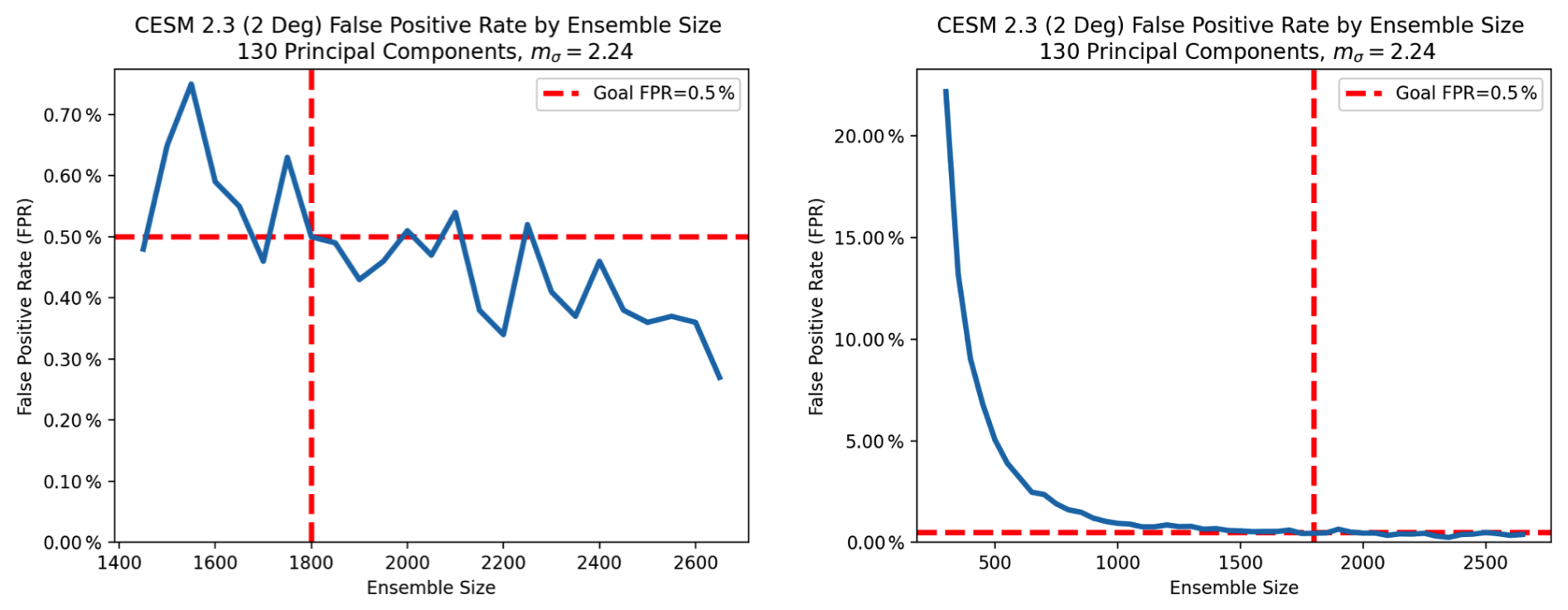
Figure 20 Experimental FPR for the UF-ECT when used with CESM 2.3, N_PC=130, and m_σ=2.24. The effects of PCA variance estimation bias can be clearly seen in the right-hand plot. While a sufficient ensemble size is key to reducing the FPR, there is a diminishing benefit to very large ensembles. Plots represents mean of 10 000 trials at each ensemble size and display the same data with different axis ranges.

With a new value for m_σ we can now test our actual FPR using samples from our base ensemble like we did before. These results are shown in left plot of Fig. 20. While there is some stochastic variation, we see that at ensemble sizes above 1800 the FPR is approximately at or below our goal of 0.5 %. It is important to consider the larger trend (shown in the right plot of Fig. 20) where the importance of sufficient ensemble size for FPR is clear. We see a diminishing benefit of increasing the ensemble size further.

Based on these results we set N_ens=1800. To summarize, we recommend the following UF-ECT test parameters for use with CESM 2.3: T=7 time steps, N_PC=130, m_σ=2.24, and N_ens=1800. While this larger ensemble represents an increase in the computational expense from what was specified in Milroy et al. (2018), it is still computationally reasonable due to the short length of the model runs and the fact they can be created in parallel. Further, because of the design of the UF-ECT, additional computation is only required when creating the model summary for the reference configuration, which is done infrequently. The work required to test new configurations against the reference configuration is the same as before.

4.4 Testing another model resolution

Models like CESM and MPAS-A are not limited to a single resolution. We now repeat our setup framework for CESM 2.3, but using the f09_f09 resolution (“1-degree”). As providing distinct test parameters for every resolution would be a significant burden for users, we then ask if the magnitude of differences is minimal enough to justify a single set of recommendations across resolutions.

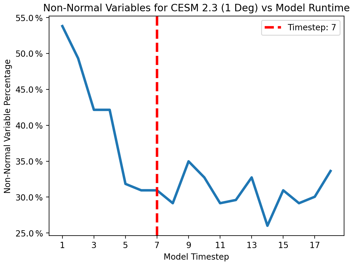
Figure 21 Non-normal variables (those with Shapiro–Wilk p score < 0.5) compared to model run length for 1-degree CESM 2.3. It appears that seven time steps (marked with a vertical red line) is again appropriate as the point at which the quantity of non-normal variables stabilizes.

Again, our setup framework begins with a large experimental ensemble of 2750 members. Using this experimental ensemble we specify an appropriate length to run the model for. In Fig. 21 we identify the point at which the number of non-normal variables stabilizes. It appears that seven model time steps is again a reasonable selection for the model run length. Again, this step may require additional knowledge of the model design. Because some variables are only updated on odd time steps in CESM 2.3, we only consider those lengths.

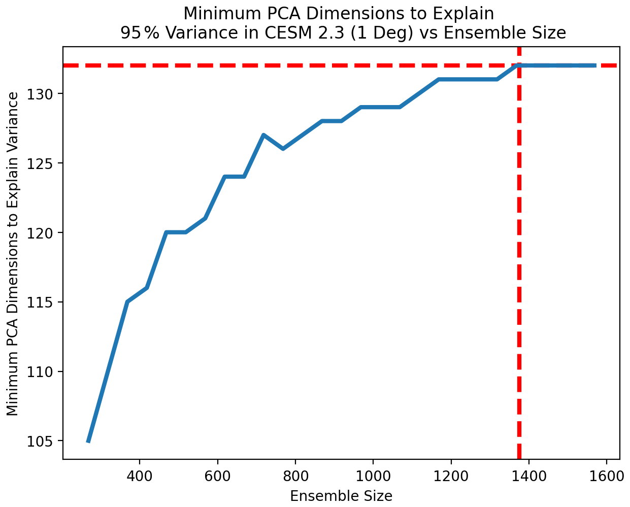
Figure 22 Number of PC dimensions needed to explain 95 % of the variance in 1-degree CESM 2.3 at time step 7 compared with sample size. We see the number of PCs stabilize at 133 beyond an ensemble size of 1375. This is an increase from the 130 PCs recommended for the 2-degree model configuration. However, the variance explained by those additional three PC dimensions is small. With 1400 runs of 1-degree CESM 2.3, the estimated variance explained by 130 PC dimensions is 94.8 %. This difference from our goal of 95 % is small enough to justify the use of the same number of PCs across resolutions. The reported value represents a 10-trial mean.

Using a model run length of T=7 time steps, we move to the next step of the setup framework where we determine the number of PC dimensions needed to accurately characterize the model. As small ensemble sizes will underestimate the variance explained by later PC dimensions we increase the ensemble size until the estimate of the number of PC dimensions required to explain 95 % of the variance stabilizes. We see in Fig. 22 that our estimate stabilizes at 133 PCs beyond an ensemble size of 1400.

With the 2-degree CESM 2.3 runs we found that our estimate stabilized at 130 PC dimensions, so the change in resolution has resulted in a different recommendation here. However, when considering our goal of accurately characterizing our model's behavior we may reasonably ask how much additional variance is explained by those additional three PC dimensions. It turns out that when using 1400 samples, the first 130 PC dimensions explain 94.8 % of the 1-degree model variance. Given how close this value is to our goal of 95 %, it is reasonable to use the same number of PC dimensions for both resolutions.

Figure 23 Experimental FPR for the UF-ECT when used with the 1-degree CESM 2.3 model, N_PC=130, and m_σ=2.24. While the estimated FPR at an ensemble size of 1800 is larger than our goal of 0.5 %, the difference is small (roughly 0.1 %). We can see in the right-hand plot that we are clearly in a similar region. Plots represent a mean of 10 000 trials at each ensemble size and display the same data with different axis ranges.

Using the same N_PC=130 means that we also will use the same value for the acceptance region, m_σ=2.24. Our final task is to ensure that our ensemble size is large enough to limit our FPR to a sufficiently low value. The experimental FPR values for 1-degree CESM 2.3 are seen in Fig. 23. While the experimental FPR is slightly higher for the 1-degree runs than the 2-degree runs at 1800 ensemble members, the difference is small (0.6 % vs 0.5 % FPR). The difference is especially minor when comparing the overall effect of ensemble size in the right-hand plot. Therefore we also find the use of an ensemble size of 1800 reasonable for 1-degree runs.

Overall, we see small differences between the recommended UF-ECT parameters for 2-degree and 1-degree CESM 2.3 runs. The exact cause of these differences is unknown but may be explored in future work. However, based on the magnitude of the differences it is reasonable to expect they will have a minimal impact on the test's effectiveness. This justifies the use of one set of UF-ECT parameters across multiple CESM resolutions. Users of other models may find this sufficient justification to only use the setup framework for a single resolution and employ the determined parameters across other resolutions. However, if a user is unsure whether the impact of resolution in their model is likely to be similar to CESM, they could also follow the setup framework with a second resolution and compare as done here.

5 MPAS-A UF-ECT testing results

In order to be considered effective, our setup framework must produce test parameters that enable the UF-ECT to properly return a failure for changes known to produce statistically distinct output. In addition, changes without statistically distinct outputs should rarely be categorized as failures (at or less than our goal FPR of 0.5 %). Generating such test cases is not an easy task. In past works (Baker et al., 2015; Milroy et al., 2018) most tests have been suggested by model developers. We take a similar approach here while also being able to rely on tests used in previous works.

As in Milroy et al. (2018), test behavior is analyzed using an approach known as the exhaustive ensemble test (EET), where 30 model runs are conducted for each change and the percentage of possible combinations of three runs (4060 total possible) that would fail the full UF-ECT procedure (EET failure rate) is reported. As discussed before, due to the stochastic nature of the UF-ECT test, a failure rate of 0 % is not expected even when runs are generated from the same configuration.

The reference configuration for all tests was created using MPAS-A v7.3 with NCAR's Cheyenne computing cluster, using the default Intel compilers (2022.1), 36 computing cores, and -O3 compiler optimization level.

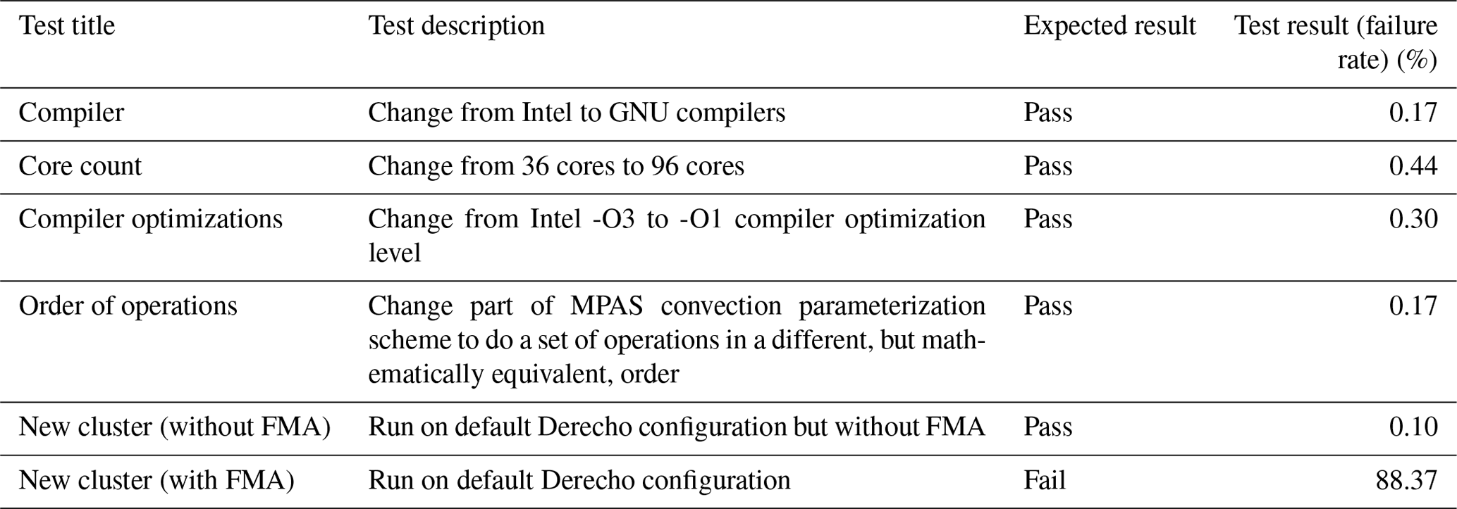
Table 1 UF-ECT MPAS-A testing results using non-scientific modifications. The UF-ECT with prescribed parameters detects expected failures while avoiding erroneous false positives.

5.1 Changes expected to pass

Changes we expect to pass include the type of non-scientific configuration changes that a model user would commonly encounter. These include changing compilers, compiler optimization levels, or the number of cores the model is run with. This also includes running on a different cluster entirely (here using NCAR's Derecho machine). Finally, we tested a code change that reordered operations in a mathematically equivalent way. We see in Table 1 that all test scenarios expected to pass do so with an FPR below our goal of 0.5 %.

5.2 Changes expected to fail

A non-scientific change that failed resulted from running the model on the Derecho computing cluster at NCAR with default compiler options. This change is representative of the type that originally inspired the ECT approach, so its failure could be concerning. But, similar to results seen in the original UF-ECT work (Milroy et al., 2018), this failure is actually due to the use of the fused multiply–add (FMA) operation. This hardware-enabled option, which allows a multiplication and subsequent addition to happen with a single rounding step, is, by default, turned off on Cheyenne but used on Derecho. While the exact mechanism by which FMA affects results is still unclear, this result is consistent with previous results.

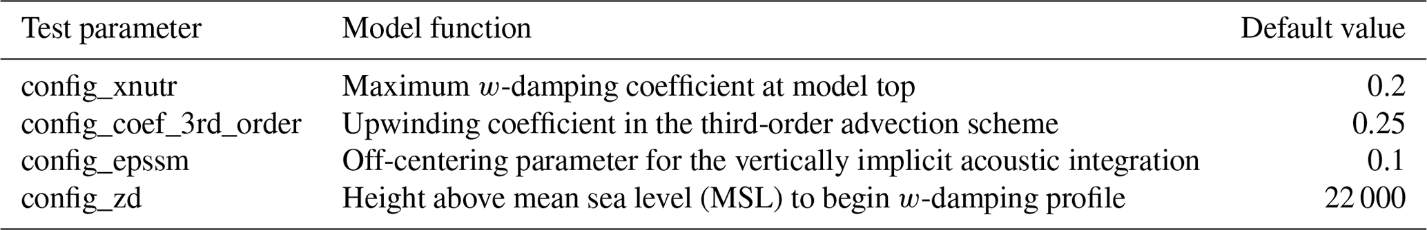
Table 2 MPAS-A scientific model parameters used for UF-ECT testing.

We initially hoped to test the impact of a change from double to single precision. Model developers of both MPAS-A and CESM believed changing precision in such a way should fail. In earlier work (Milroy et al., 2018) a precision-based test scenario passed the UF-ECT for CESM. However, in that case only one subroutine was modified, keeping field representations in double precision, whereas our change for MPAS-A would impact the entire model code.

Unfortunately, due to initial perturbations being on the order of machine epsilon for double precision, they are essentially erased when applied to a temperature field represented by single precision. This prevents the creation of independent test runs. How to effectively test configurations when the accepted ensemble used a higher level of precision than the test configuration remains an open question.

Another set of tests expected to fail includes scientific changes to the model in the form of model parameter changes. In previous ECT work (Baker et al., 2015), the model parameter changes suggested by scientists ranged in magnitude from approximately 5 % to 100 % of the original parameter values and all but one resulted in ECT failures. Each test only modified a single parameter by a fixed amount. For instance, a CESM configuration with a dust emission parameter set to 0.45 was tested against an ensemble generated with that parameter set to a default value of 0.55.

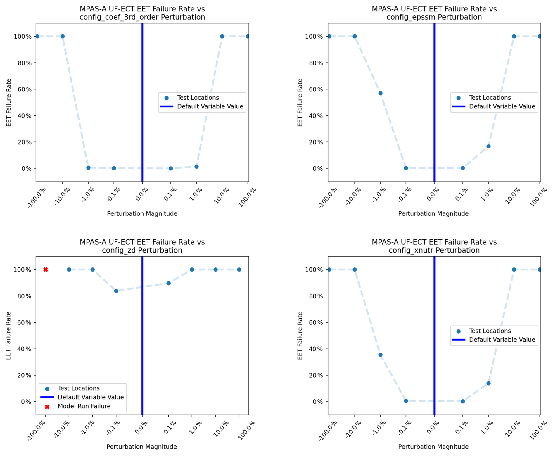
Figure 24 Average UF-ECT failure rate as a result of perturbing different physical parameters by various magnitudes. For all parameters, changes are detected when perturbation is 10 % (or more) of the default parameter value. For the parameter config_zd, perturbations as small as 0.1 % are detected.

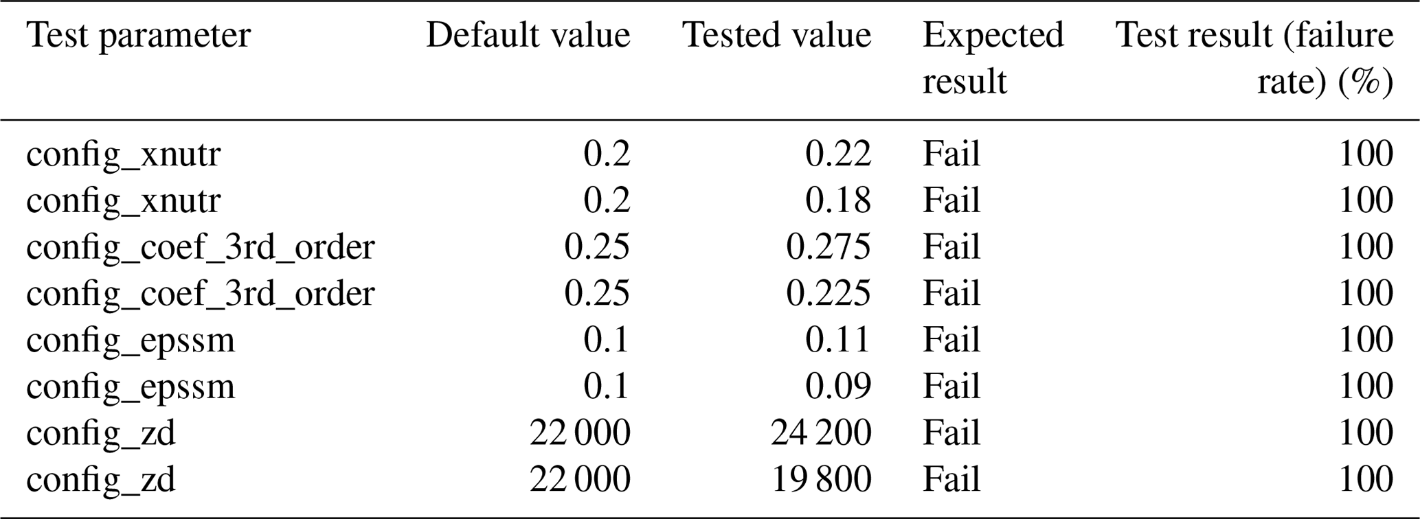
In this work we have expanded this analysis by testing the UF-ECT failure rate of four model parameters when perturbed by four different orders of magnitude (from 100 % to 0.1 % of the original parameter value) in both positive and negative directions (for another example testing the sensitivity of a test to a range of model parameters, see Mahajan, 2021). We also report the failure rate due to a change of 10 % in Table 2, analogous to previous ECT works. The sensitivity of the UF-ECT across a range of perturbation magnitudes is seen in Fig. 24.

We see a clear relationship between the degree to which the parameters were perturbed and the rate of failing the UF-ECT. Overall the test appears to be sensitive to parameter perturbations larger than 1 % to 10 % in magnitude, depending on parameter. This aligns with the magnitude of change that domain scientists expected would affect output in previous works. The damping height parameter config_zd appears to be the outlier, with UF-ECT being sensitive to changes as small as 0.1 % of the default parameter value.

Table 3 UF-ECT testing using MPAS-A scientific model parameters perturbed by 10 %.

5.3 Off by one: a realistic bug scenario

In addition to the changes noted earlier that would not be expected to give inconsistent results – running on a different machine, building the model with different compilers, and running the model using different numbers of processors – there is another important class of changes that turn up during numerical model development that should not change results, namely the refactoring of code. To demonstrate the effectiveness of the UF-ECT and its value in the model development process, we consider a hypothetical, though entirely realistic, scenario in which a small piece of code is generalized and rewritten. We compare a correct refactoring with a version where an “off-by-one” error (also known as a “fence-post” error) is introduced. This type of error is simple but common (and also quite old, having been documented by individuals as far apart as Vitruvius and Dijkstra Pollio, 1999; Dijkstra, 1982).

Numerical atmospheric models contain code to implement various filters and other dissipation methods, and in MPAS-A, one such piece of code is used to enforce a lower bound on the eddy viscosities employed by a horizontal Smagorinsky-type filter in the uppermost layers of the model. First, we consider Algorithm 1 for implementing this lower bounding, where K(n) represents the eddy viscosity at layer n in a model grid column, N_layer is the number of vertical layers (with 1-based indexing, layer N_layer represents the uppermost layer), and μ is a constant physical eddy viscosity that is controlled by a model runtime parameter.

Algorithm 1 Baseline

$K\left(N_{\text{layer}}\right)=\text{max}\mathit{\left\{}K\right(N_{\text{layer}}),\mathrm{3}/\mathrm{3}\times \mathit{\mu }\mathit{\}}$

$K(N_{\text{layer}}-\mathrm{1})=\text{max}\mathit{\left\{}K\right(N_{\text{layer}}-\mathrm{1}),\mathrm{2}/\mathrm{3}\times \mathit{\mu }\mathit{\}}$

$K(N_{\text{layer}}-\mathrm{2})=\text{max}\mathit{\left\{}K\right(N_{\text{layer}}-\mathrm{2}),\mathrm{1}/\mathrm{3}\times \mathit{\mu }\mathit{\}}$

Next, we consider Algorithm 2, a generalized version of Algorithm 1, where the algorithm has been refactored to use an arbitrary number of levels in the lower bounding.

Algorithm 2 Generalized

$i\leftarrow (N_{\text{layer}}-N_{\text{filter}}+\mathrm{1})$

while i≤N_layer  do

$K\left(i\right)=\text{max}\mathit{\left\{}K\right(i),(\mathrm{1.0}-(N_{\text{layer}}-i)/N_{\text{filter}})\times \mathit{\mu }\mathit{\}}$

end while

It may easily be verified that when N_filter=3, and under the assumption of exact arithmetic, Algorithms 1 and 2 apply identical lower bounds over the top three layers in each model grid column. When implemented in MPAS-A, however, the results from model simulations employing each of the two algorithms were found not to provide bitwise identical results with double-precision real values using the GNU 13.2.0 compilers with optimization level -O0. This is likely a result of a change in the ordering of underlying floating-point operations.

Finally, we consider Algorithm 3, a variation of the generalized lower bounding (Algorithm 2) that contains an off-by-one error (highlighted in red) in the computation of the coefficient for μ.

Algorithm 3 Generalized, with off-by-one error

$i\leftarrow (N_{\text{layer}}-N_{\text{filter}}+\mathrm{1})$

while i≤N_layer  do

$K\left(i\right)=\text{max}\mathit{\left\{}K\right(i),(\mathrm{1.0}-(N_{\text{layer}}-i+\mathrm{1})/N_{\text{filter}})\times \mathit{\mu }\mathit{\}}$

end while

Table 4 The root mean square (rms) difference and maximum pointwise absolute difference in two model fields after 30 time steps (6 h of simulated time) using Algorithms 1, 2, and 3. Simulations were done with a typical case used for initial testing in MPAS-A and employed a 120 km quasi-uniform horizontal mesh and 55 vertical layers up to a model top located 30 km above mean sea level. Test simulations were started from a “spun-up” model state saved in a checkpoint or restart file. The variable u refers to horizontal normal velocity at edges of cells. The variable w refers to vertical velocity at vertical cell faces.

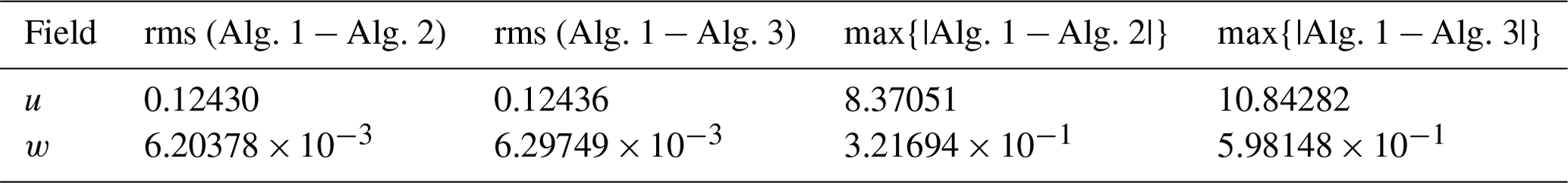
By changing the coefficients multiplied by μ, the off-by-one error in Algorithm 3 is no longer mathematically equivalent to Algorithm 1 and, as expected, produces different results numerically. However, when used in a typical test case scenario the magnitude of differences between the three algorithms is similar (see Table 4). This prevents the easy identification of refactoring errors.

The scenario described here is not unrepresentative of those that occur in the course of typical model development. When refactored model code produces bitwise identical results, the modified code is often accepted, but when there are even small differences in results without compiler optimizations, deeper investigation is often needed in order to ascertain whether the refactored code has introduced an error. In this example, two simple metrics – rms difference and maximum pointwise absolute difference – shown in Table 4 are of the same order of magnitude when considering “correct” code and “incorrect” code, and it might therefore be difficult for a model developer to determine whether their generalized code was in fact correct.

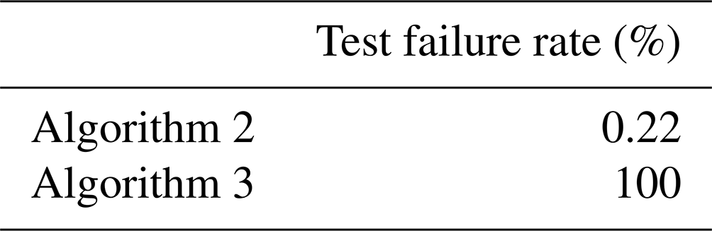
In contrast, when Algorithms 2 and 3 are compared to Algorithm 1 using UF-ECT, the results very clearly indicate the faulty version (Table 5). These results demonstrate the usefulness of UF-ECT for identifying common refactoring mistakes when BFB equivalence is not possible and basic tests (like those described in Table 4) fail to provide conclusive results. In practice, the UF-ECT has recently proven valuable for catching errors introduced when refactoring CESM code for GPUs.

Table 5 UF-ECT test failure rates of Algorithms 2 and 3. In this setup, Algorithm 1 was used to create the accepted ensemble and other UF-ECT test parameters were specified as described earlier in the paper. UF-ECT is able to correctly return a fail result for the algorithm containing an off-by-one error while passing the correctly refactored code.

6 Key lessons learned

6.1 Output variable selection is key

A foundational assumption of the UF-ECT method is that the output variables used to run the test effectively represent the behavior of the numerical model. This means they must be diverse and important enough to the model that they will capture the impact of any bug or unexpected configuration change. But every model may have different norms about what is included in default output variables. Some models may be set up to output few variables, assuming users will add outputs for any relevant science. Other models may be designed to output almost everything by default, relying on users to remove fields they do not find useful. While UF-ECT helps reduce the need for domain expertise during testing, knowledge from model developers is still key to ensuring that the output variables provide good coverage of model behavior.

6.2 Accounting for PCA variance estimation bias is vital

The bias in estimating a PC dimension's variance, described in Sect. 2.2, is often ignored when PCA is used for other purposes. For example, if a data scientist only cares about finding linear combinations of variables with high variance, then the bias is unlikely to matter much for their work (though the bias should probably be accounted for more when deciding how many PC dimensions to use, similar to our approach in Sect. 3.4).

In contrast, the UF-ECT approach specifically relies on the distribution of those linear combinations across the ensemble of numerical model runs. The mean and spread of PC dimensions are what determine whether the outputs of a new model configuration pass or fail. As we have shown here, ignoring the bias and not accounting for it through test parameter choices and ensemble size can cause high rates of erroneous failures, known as false positives. This lesson should apply for similar approaches as well. When a method relies on characterizing the distribution of PCs, as the UF-ECT does, then accounting for bias in the variance of those distributions becomes extremely important.

6.3 Non-scientific changes can have a similar effect as scientific ones

Our results from applying UF-ECT to MPAS-A emphasize the fact that both scientific and non-scientific modifications can affect model output to similar degrees (when viewed in the distributional sense of UF-ECT). To have a rather innocuous modification like FMA be as impactful as changing a scientific model parameter by 1 % to 10 % may take some model developers by surprise. But, in fact, this issue appears for similar changes in other codes (Ahn et al., 2021).

These results prompt a variety of questions. The exact way in which FMA affects the distribution of a chaotic model's outputs is still unknown. Past work (Milroy et al., 2018) has shown good agreement between changes detected using the ultrafast runs and year-long runs. Further exploration of the effect of non-scientific changes on long runs is warranted.

The presence of test failures due to FMA is also a reminder that UF-ECT cannot tell us which particular configuration of a model is correct. In theory, enabling FMA should result in more accurate results due to the fewer rounding steps. UF-ECT failures just indicate that a statistically significant difference exists. The exact nature of how these configuration changes affect scientific computer models is a question for future work. What we know is this: numerical configuration decisions can easily affect model outputs as much as scientific ones.

7 Conclusions

In this work we have developed a generalized setup framework for specifying necessary test parameters for the UF-ECT method when applying it to different or updated scientific models. This approach was based on an in-depth examination of the effect of each parameter on the effectiveness of the test, with particular attention paid to the effects of PCA variance estimation bias. UF-ECT test parameters were specified for the MPAS-A atmospheric model as well as the most recent version of CESM with the CAM atmospheric component. We showed that changes to model resolution are unlikely to have a significant impact on the test effectiveness.

We also demonstrated the performance of the specified test parameters using the MPAS-A atmospheric model with a variety of realistic test scenarios. This testing demonstrated the effectiveness of the test while also giving insight into the power of non-scientific configuration changes for model outputs.

In future work we plan to develop better tools for analyzing test failures when they do occur. The Ruanda tool (Milroy et al., 2019; Ahn et al., 2021) makes significant progress toward the goal of providing insight into the cause of a test failure, but more work is needed to better enable its use in practice. Deeper investigation into the effects of FMA or precision changes will help further our understanding of how non-scientific model changes affect output distributions. This will be useful not just for designing effective consistency testing methods, but also determining how models should be implemented numerically and run.

As numerical scientific models continue to grow in size and complexity, and the computing platforms they are run on become less deterministic, the need for efficient, objective consistency testing will only grow. The generalized setup framework developed in this work will enable new users to easily apply an ultrafast ensemble-based consistency testing approach to their own models, enabling this powerful technique to be used outside the CESM community.