Sensitivity studies of a four-dimensional local ensemble transform Kalman filter coupled with WRF-Chem version 3.9.1 for improving particulate matter simulation accuracy

Accurately simulating severe haze events through numerical models remains a challenge because of uncertainty in anthropogenic emissions and physical parameterizations of particulate matter (PM_2.5 and PM₁₀). In this study, a coupled Weather Research and Forecasting with Chemistry (WRF-Chem)–four-dimensional local ensemble transform Kalman filter (4D-LETKF) data assimilation system has been successfully developed to optimize particulate matter concentration by assimilating hourly ground-based observations in winter over the Beijing–Tianjin–Hebei (BTH) region and surrounding provinces. The effectiveness of the 4D-LETKF system and its sensitivity to the ensemble member size and length of the assimilation window are investigated. The promising results show that significant improvements have been made by analysis in the simulation of particulate matter during a severe haze event. The assimilation reduces root mean square errors in PM_2.5 from 69.93 to 31.19 µg m⁻³ and of PM₁₀ from 106.88 to 76.83 µg m⁻³. Smaller root mean square errors and larger correlation coefficients in the analysis of PM_2.5 and PM₁₀ are observed across nearly all verification stations, indicating that the 4D-LETKF assimilation optimizes the simulation of PM_2.5 and PM₁₀ concentration efficiently. Sensitivity experiments reveal that the combination of 48 h of assimilation window length and 40 ensemble members shows the best performance for reproducing the severe haze event. In view of the performance of ensemble members, an increasing ensemble member size improves ensemble spread among each forecasting member, facilitates the spread of state vectors about PM_2.5 and PM₁₀ information in the first guess, favors the variances between each initial condition in the next assimilation cycle, and leads to better simulation performance in both severe and moderate haze events. This study advances our understanding of the selection of basic parameters in the 4D-LETKF assimilation system and the performance of ensemble simulations in a particulate-matter-polluted environment.

1 Introduction

Although great progress regarding air pollution control has been made during recent years, China is facing the highest levels of particulate matter in the world (van Donkelaar et al., 2016). Particulate matter consists of PM_2.5 and PM₁₀, referring to particles with aerodynamic diameters of less than 2.5 and 10 µm, respectively. A high concentration of particulate matter is a major factor for severe haze events (air quality index larger than 200) in the Beijing–Tianjin–Hebei (BTH) region of China, especially during winter (Yan et al., 2016; Zhang et al., 2018). Numerical models are considered to be useful tools for simulating haze events as they take complex physical and chemical mechanisms into account, but the uncertainty in emissions and physical parameterizations still remains a significant barrier in improving the simulation accuracy (Gao et al., 2017; Feng et al., 2018).

As an effective statistical approach, data assimilation is capable of improving the accuracy of pollution simulations by limiting the performance of models. A lot of data assimilation approaches have been applied to atmospheric science, including three-dimensional variation (3D-Var) (Lorenc, 1986; Parrish and Derber, 1992; Sun et al., 2020), four-dimensional variation (4D-Var) (Huang et al., 2009; Benedetti et al., 2009), and ensemble Kalman filter algorithms and their variants (Evensen, 1994; Whitaker and Hamill, 2002; Miyazaki et al., 2012a). Among them, four-dimensional local ensemble transform Kalman filter (4D-LETKF) has shown unique characteristics in numerical simulation (Evensen, 2003; Kong et al., 2021). Firstly, derived from finite-forecasting members, the background error covariance matrix of 4D-LETKF features flow-dependent characteristics, and the linear combinations of ensemble members produce a global analysis (Hunt et al., 2007). Secondly, the computational time for 4D-LETKF remains robust as the observation numbers increase, exhibiting strong computational ability in the parallel architecture when assimilating various measurements (Miyoshi et al., 2007; Hunt et al., 2007; Dai et al., 2021). Lastly, 4D-LETKF can assimilate time slots of asynchronous observations to optimize the current state within the assimilation window, which efficiently improves the quality of pollution prediction (Evensen, 2003; Ott et al., 2004; Dai et al., 2019; Cheng et al., 2019).

The characteristics of 4D-LETKF underscore the importance of the ensemble member size and length of the assimilation window for its effectiveness. The background error covariance matrix, which represents the uncertainty in the ensemble simulations, is determined by the spread of the ensemble members (Peng et al., 2017). In general, 4D-LETKF considers approximate model trajectories by observing linear combinations of the background ensemble trajectories. However, limited numbers of ensemble members may bring about insufficient dispersion of ensemble systems (Hunt et al., 2004). Overall, the 4D-LETKF system can greatly improve the utilization rate of observations by constraining the state variables in an asynchronous hourly slot within the assimilation window. A longer assimilation window efficiently reduces the computational load by avoiding frequent switches between state and forecast variables. But the trajectories in a long assimilation window may diverge enough that linear combinations will not approximate the model trajectories. Moreover, the model ensemble trajectory may not fit the observations well over the entire interval with the presence of model errors (Dai et al., 2019). Many studies have discussed the choice of these two parameters for ensemble Kalman filter algorithms and their variants. When optimizing hourly aerosol fields by satellite observations, Cheng et al. (2019) revealed that the forecast with a 24 h assimilation window was comparable to those with 1 h; the root mean square error for aerosol optical depth (AOD) is 0.091 and 0.110, respectively, indicating the weights determined at the end of the 24 h assimilation window are valid to optimize the ensemble trajectories. However, Dai et al. (2019) proposed that over 80  % of the hourly assimilation efficiencies for the 1 h assimilation window are higher than those with 6 or 24 h in 4D-LETKF experiments, suggesting that assimilation efficiency decreases with the increase in the assimilation window interval. These different opinions reveal that there is still a large uncertainty in the selection of parameters in the 4D-LETKF assimilation system.

The accuracy simulation of severe haze events with air quality index (AQI) larger than 200 has been a challenging problem for a long time, posing severe threats to human daily life and public health (Wang et al., 2014; Kong et al., 2021; Gao et al., 2017). Although 4D-LETKF has unique advantages in computational efficiency and analysis, there is little research that investigates the impacts of 4D-LETKF assimilation on pollutant simulations, especially in severe haze events; in addition, it is also imperative to explore the basic optimal combination of assimilation parameters and its explanation in this method. Our major objectives are to not only evaluate the performance of 4D-LETKF in reproducing particulate matter concentration during a severe haze event, but also summarize the influence rules of ensemble size and assimilation window length on particulate matter simulation and explore whether these rules are applicable to a moderate haze event (air quality index smaller than 200) as well. The results have great significance for verifying and quantifying the effect of 4D-LETKF assimilation on numerical simulations of PM_2.5 and PM₁₀, subsequently providing a general rule for parameter selection in the 4D-LETKF during severe haze events. Herein, we utilize the 4D-LETKF system, which is coupled with the Weather Research and Forecasting with Chemistry (WRF-Chem) model to improve simulative skill of particulate matter among northern China during the winter of 2020. Section 2 briefly introduces detail setting of WRF-Chem model, 4D-LETKF, observations and numerical experiment designs. Section 3 compares the assimilation with those in the prior simulation, summarizes and explains sensitivity rules for parametric selection, and followed by a conclusion in Sect. 4 lastly.

2 Methodology

2.1 Configuration of the forecast model

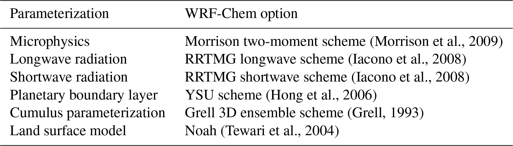
In our implementation, the fully coupled online WRF-Chem version 3.9.1 is employed as a numeral forward model to describe the meteorological and chemical conditions simultaneously, in which it fully considers extensive chemical transport processes including advection, convection and sedimentation processes (Grell et al., 2005). The WRF-Chem model is configured with two domains (d01 and d02), both using 100 (west–east) × 100 (south–north) grid points but with horizontal resolutions of 30 and 10 km, respectively. As shown in Fig. 1a, the d01 domain covers most of east Asia, and the area under the blue shadow is the d02 domain. The vertical grid contains 40 full sigma levels, extending from the surface to 50 hPa.

The initial and lateral boundary conditions of meteorological fields are derived from the National Centers for Environmental Prediction Final (NCEP FNL) analysis data with a spatial resolution of 1° × 1° and temporal interval of 6 h. A state-of-the-art and highly non-linear gas-phase chemical mechanism Regional Atmospheric Chemistry Mechanism (RACM) (Stockwell et al., 1997) is selected as the gas-phase mechanism, and Goddard Chemistry Aerosol Radiation and Transport (GOCART) (Schwartz et al., 2012) is adopted as the aerosol mechanism. The parameterization scheme used in research is shown in Table 1.

Table 1 WRF-Chem parameterization scheme in this study. RRTMG stands for Rapid Radiative Transfer Model for General Circulation Models, and YSU stands for Yonsei University.

The anthropogenic emissions are obtained from the Multi-resolution Emission Inventory for China (MEIC, 2024) compiled by Tsinghua University. The inventory includes anthropogenic emissions from agriculture, industry, power, residential, and transportation sectors (Zheng et al., 2021). The inventory has a spatial resolution of 0.25° × 0.25° and has been interpolated to match the simulation resolution. The biogenic emissions are calculated online by Guenther scheme (Guenther et al., 1995). The PM_2.5, PM₁₀ concentrations output from WRF-Chem are linearly interpolated to site observations. The evaluation of uncertainty in the emission inventory has been shown in previous research (Zhang et al., 2009).

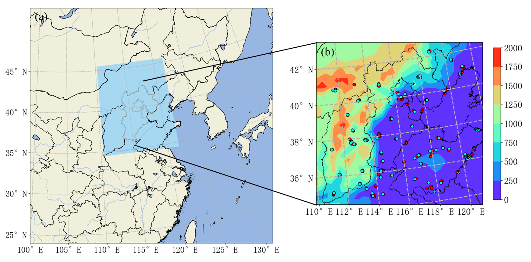
Figure 1 (a) WRF-Chem model domains. The grey border implies the BTH region. (b) Location of assimilated and independent verification observation sites with topography (m). The red and blue dots imply the assimilated and independent verification observation site, respectively. Publisher's remark: please note that the above figure contains disputed territories.

2.2 The 4D-LETKF algorithm and the state variables

The 4D-LETKF coupled with the WRF-Chem model is implemented to investigate the influence of assimilation on particulate matter simulation in this research. In this section, we introduce the 4D-LETKF algorithm and corresponding state variables briefly, a more detailed information can be found in Hunt et al. (2007). The LETKF features a flow-dependent covariance matrix from ensemble simulation and determines the analysis ensemble mean, ${\stackrel{\mathrm{‾}}{x}}^{\mathrm{a}}$ (a posteriori), according to the following formula:

$$\begin{array}{}\text{(1)}& {\stackrel{\mathrm{‾}}{x}}^{\mathrm{a}}={\stackrel{\mathrm{‾}}{x}}^{\mathrm{b}}+{\mathbf{X}}^{\mathrm{b}}{\stackrel{\mathrm{‾}}{w}}^{\mathrm{a}},\end{array}$$

where ${\stackrel{\mathrm{‾}}{x}}^{\mathrm{b}}$ and X^b denote the ensemble mean of the first guess and background ensemble perturbations, respectively. The ensemble perturbation matrix (X^b) is calculated by $x^{\mathrm{b}}\left(i\right)-{\stackrel{\mathrm{‾}}{x}}^{\mathrm{b}}\mathit{\{}i=\mathrm{1},\mathrm{2},\mathrm{\dots },k\mathit{\}}$, where k represents the ensemble member size. The perturbation weight matrix ${\stackrel{\mathrm{‾}}{w}}^{\mathrm{a}}$ is the Kalman gain which linearly determines the increment between the analysis and the first guess, and can be calculated as follows:

$$\begin{array}{}\text{(2)}& {\stackrel{\mathrm{‾}}{w}}^{\mathrm{a}}={\stackrel{\mathrm{̃}}{P}}^{\mathrm{a}}{\left(Y^{\mathrm{b}}\right)}^T{\mathbf{R}}^{-\mathrm{1}}({\mathit{y}}^{\mathrm{0}}-{\stackrel{\mathrm{‾}}{y}}^{\mathrm{b}}),\end{array}$$

where ${\stackrel{\mathrm{̃}}{P}}^{\mathrm{a}}$ is the analysis error covariance in ensemble space. y⁰ and ${\stackrel{\mathrm{‾}}{y}}^{\mathrm{b}}$ denote the observations vector and ensemble mean background observations, respectively. Ensemble mean background observations derived from applying the observation vector to the ensemble member state vector H (${\stackrel{\mathrm{‾}}{x}}^{\mathrm{b}})$. The matrix R is the observation error covariance matrix. The matrix Y^b represents ensemble background observation perturbations, whose ith column is $y^{\mathrm{b}}\left(i\right)-{\stackrel{\mathrm{‾}}{y}}^{\mathrm{b}}$, $\mathit{\{}i=\mathrm{1},\mathrm{2},\mathrm{\dots },k\mathit{\}}$. ${\stackrel{\mathrm{̃}}{P}}^{\mathrm{a}}$ can be obtained as follows:

$$\begin{array}{}\text{(3)}& {\stackrel{\mathrm{̃}}{P}}^{\mathrm{a}}=[\left(k-\mathrm{1}\right)\mathbf{I}/\mathit{\rho }+({\mathbf{Y}}^{\mathrm{b}}{)}^T{\mathbf{R}}^{-\mathrm{1}}{\mathbf{Y}}^{\mathrm{b}}{]}^{-\mathrm{1}},\end{array}$$

where I denotes the identity matrix and k is ensemble member size. The multiplicative inflation factor ρ is necessary to avoid the filter divergence (Anderson and Anderson, 1999; Sekiyama et al., 2010), which is set to 1.1 to inflate the analysis covariance (Dai et al., 2019; Anderson, 2007). Analysis ensemble perturbation (X^a) is calculated by

$$\begin{array}{}\text{(4)}& X^{\mathrm{a}}={\mathbf{X}}^{\mathrm{b}}{\left[(k-\mathrm{1}){\stackrel{\mathrm{̃}}{P}}^{\mathrm{a}}\right]}^{\mathrm{1}/\mathrm{2}}={\mathbf{X}}^{\mathrm{b}}{W}^{\mathrm{a}}.\end{array}$$

Calculated by the sum of the ${\stackrel{\mathrm{‾}}{x}}^{\mathrm{a}}$ and each of the columns of X^a, the ensemble analyses are served as optimal initial conditions in each ensemble member to generate the first guess in the next cycle.

Figure 2 is the flow chart of the WRF-Chem–4D-LETKF assimilation system applied in our implementation. The system conducts these processes within each assimilation cycle. The 4D-LETKF generates a flow-dependent background error covariance matrix by ensemble member. Given that the emissions inventory is an important source of uncertainty in simulation (Pagowski and Grell, 2012), the research randomly perturbs anthropogenic emissions of PM, black carbon (BC), and organic carbon (OC) in January for each member to create the ensemble members, and the perturbation follows a log-normal distribution in the k-dimensional space. The mean values of perturbations of PM_2.5, PM₁₀, BC, and OC emissions are equal to 1, and the variances of these emissions are set according to corresponding uncertainty in MEIC inventory (130 %, 132 %, 208 %, and 258 % for PM_2.5, PM₁₀, BC, and OC, respectively) (Luo et al., 2023). Such ensemble anthropogenic emissions are perfectly correlated in spatial and temporal dimension and should not be regarded as overly restrictive (Schutgens et al., 2010; Dai et al., 2021). This study only adds perturbations one time into emissions at the first cycle of assimilation to provide the information spread of particulate matter. It is enough to make the most out of the site information affecting the first-guess field. The WRF-Chem–4D-LETKF system propagates the ensemble forward simulation for the entire assimilation window time and outputs the first-guess fields at each hourly time slot. The ensemble mean of the first guess (${\stackrel{\mathrm{‾}}{x}}^{\mathrm{b}}$) and background ensemble perturbations (X^b) can be obtained from the ensemble member here. Combining the observation and the observation operator, the innovation (${\mathit{y}}^{\mathrm{0}}-{\stackrel{\mathrm{‾}}{y}}^{\mathrm{b}}$) and Y^b can be obtained in each time slot. The perturbation weight matrix (${\stackrel{\mathrm{‾}}{w}}^{\mathrm{a}}$) is valid within a relative short assimilation window (e.g., 24 or 48 h) (Hunt et al., 2004; Cheng et al., 2019). The analysis ensemble derived from ${\stackrel{\mathrm{‾}}{w}}^{\mathrm{a}}$ at the end of time slots will serve as chemical initial conditions for the next assimilation window. As the cycle of assimilation proceeds, a linear combination of the analysis ensemble is continuously obtained.

Figure 2 Flow chart of the WRF-Chem–4D-LETKF assimilation system for particulate matter.

The ensemble Kalman filter generally encounters a spurious long-distance correlation problem because of the limited numbers of ensemble members (Miyazaki et al., 2012a). To avoid the problem above, it is necessary to apply observation localizations to filter observations from a long distance. Overall, 4D-LETKF offers a flexible choice of observation localizations in horizontal, vertical, and temporal dimensions for each grid point (Cheng et al., 2019). In this study, the horizontal localization factor is calculated as the Gaussian function (Miyoshi et al., 2007), which gradually reduces the effect of observations as the increasing departure from the analysis grid:

$$\begin{array}{}\text{(5)}& f\left(r\right)=\exp (-r^{\mathrm{2}}/\mathrm{2}{\mathit{\sigma }}^{\mathrm{2}}).\end{array}$$

Here, r represents the physical distance from the observation to the analysis grid, and σ represents localization length. We limit the localization factor from 0 to 3.65 times the localization length (Zhao et al., 2015), ignoring the observation beyond 3.65 times the localization length to the analysis grid.

The selection of the state variables depends on the generative mechanism of aerosol. As a result, 16 kinds of WRF-Chem–GOCART aerosol variables are treated as state variables. For the PM_2.5 observations, the observation operator is described as follows:

$$\begin{array}{}\text{(6)}& \begin{array}{rl}{y}_{{\mathrm{PM}}_{\mathrm{2.5}}}^{\mathrm{b}}& ={\mathit{\rho }}_{\mathrm{d}}[P_{\mathrm{2.5}}+\mathrm{1.375}S+\mathrm{1.8}({\mathrm{OC}}_{\mathrm{1}}+{\mathrm{OC}}_{\mathrm{2}})\\ & +{\mathrm{BC}}_{\mathrm{1}}+{\mathrm{BC}}_{\mathrm{2}}+D_{\mathrm{1}}+\mathrm{0.286}{D}_{\mathrm{2}}+S_{\mathrm{1}}+\mathrm{0.942}{S}_{\mathrm{2}}],\end{array}\end{array}$$

where ρ_d represents the dry-air density; P_2.5 is the fine unspecified aerosol contribution; S represents sulfate; and OC₁ and OC₂ are hydrophobic and hydrophilic organic carbon, respectively.

BC₁ and BC₂ are hydrophobic and hydrophilic black carbon, D₁ and D₂ are dusts with effective radii of 0.5 and 1.4 µm, and S₁ and S₂ are sea salts with effective radii of 0.3 and 1.0 µm, respectively (Peng et al., 2018).

Similarly, the observation operator for PM₁₀ is shown as follows:

$$\begin{array}{}\text{(7)}& \begin{array}{rl}{y}_{{\mathrm{PM}}_{\mathrm{10}}}^{\mathrm{b}}& ={\mathit{\rho }}_{\mathrm{d}}[P_{\mathrm{10}}+P_{\mathrm{2.5}}+\mathrm{1.375}S+\mathrm{1.8}({\mathrm{OC}}_{\mathrm{1}}+{\mathrm{OC}}_{\mathrm{2}})\\ & +{\mathrm{BC}}_{\mathrm{1}}+{\mathrm{BC}}_{\mathrm{2}}+D_{\mathrm{1}}+\mathrm{0.286}{D}_{\mathrm{2}}+D_{\mathrm{3}}+\mathrm{0.87}{D}_{\mathrm{4}}\\ & +S_{\mathrm{1}}+\mathrm{0.942}{S}_{\mathrm{2}}+S_{\mathrm{3}}],\end{array}\end{array}$$

where P₁₀ is the coarse unspecified aerosol contribution and D₃ and D₄ are dusts with effective radii of 2.4 and 4.5 µm. S₃ is sea salt with an effective radius of 3.2 µm. Therefore, the simulated PM_10–2.5 is

$$\begin{array}{}\text{(8)}& y_{{\mathrm{PM}}_{\mathrm{10}\text{–}\mathrm{2.5}}}^{\mathrm{b}}={\mathit{\rho }}_{\mathrm{d}}[P_{\mathrm{10}}+D_{\mathrm{3}}+\mathrm{0.87}{D}_{\mathrm{4}}+S_{\mathrm{3}}].\end{array}$$

In this research, $y_{{\mathrm{PM}}_{\mathrm{10}\text{–}\mathrm{2.5}}}^o$ calculated using $y_{{\mathrm{PM}}_{\mathrm{10}}}^o-y_{{\mathrm{PM}}_{\mathrm{2.5}}}^o$ is used to analyze state variables including D₅ and S₄, which are dust with effective radii of 8 µm and sea salt with effective radii of 7.5 µm, respectively.

2.3 Site observation data and errors

Ground-based observations feature a high temporal resolution, which can capture variation in pollution concentration on an hourly scale at the bottom of the troposphere, providing continuous and reliable observations. The quality-assured and quality-controlled hourly observation data of PM_2.5 and PM₁₀ are used to explore the influence of 4D-LETKF assimilation in this research. The pollution data were obtained from the China National Environmental Monitoring Center (CNEMC, 2024). As the research primarily focuses on the BTH region, the assimilation and verification sites are mainly located in the BTH region and neighboring provinces, primarily in urban and suburban areas. In order to obtain more reliable observation data, the quality control of observation data in this study includes hourly observations of default value and extreme value detection. First, during the haze period, if the number of missing values for either type of pollutant at one site exceeds 24 h, this site is considered to have a certain uncertainty in observation quality, and data will not be assimilated. Second, for each kind of observation in different station, the hourly observations outside the range of m±3σ, where the m and σ are the mean value and standard deviation of daily concentration, respectively, will not be assimilated. When selecting assimilation and verification sites, spatial distribution uniformity is ensured for better assimilation performance; consequently, those sites are randomly selected. Finally, 127 assimilation sites and 69 verification sites in the BTH region and surrounding provinces are selected (Fig. 1b). It can be seen that the assimilation and verification sites have a relatively uniform spatial distribution.

The observation error covariance matrix (R) is assumed to be diagonal, implying that observational errors among each pollution species are uncorrelated. The observation error (r) consists of the measurement error (ε₀) and the representation error (ε_r):

$$\begin{array}{}\text{(9)}& r=\sqrt{{\mathit{\epsilon }}_{\mathrm{0}}^{\mathrm{2}}+{\mathit{\epsilon }}_r^{\mathrm{2}}}.\end{array}$$

The measurement error (ε₀) is defined as

$$\begin{array}{}\text{(10)}& {\mathit{\epsilon }}_{\mathrm{0}}=\mathrm{ermax}+\mathrm{0.0075}\times {\mathrm{\Pi }}_{\mathrm{0}},\end{array}$$

where ermax is the base error, which is set to 1 for PM_2.5 and PM₁₀ (Chen et al., 2019a), and Π₀ denotes the observation of concentration. Produced by the observation operator, the representation error can be calculated by the following formula (Elbern et al., 2007):

$$\begin{array}{}\text{(11)}& {\mathit{\epsilon }}_r=\mathit{\gamma }{\mathit{\epsilon }}_{\mathrm{0}}\sqrt{\mathrm{\Delta }l/L},\end{array}$$

where γ is the tunable scaling factor set to 0.5, Δl is the spatial resolution of gridding (30 and 10 km for d01 and d02, respectively), and L depends on station location, which denotes the range that an observation can reflect; here, L is 2 km for this calculation.

Meteorological data were collected from the National Climatic Data Center (NCDC, 2024), which provides the hourly air temperature, dew point, and wind speed data. The observational meteorological data are used to validate the performance of the simulations in this study.

2.4 Experiment design

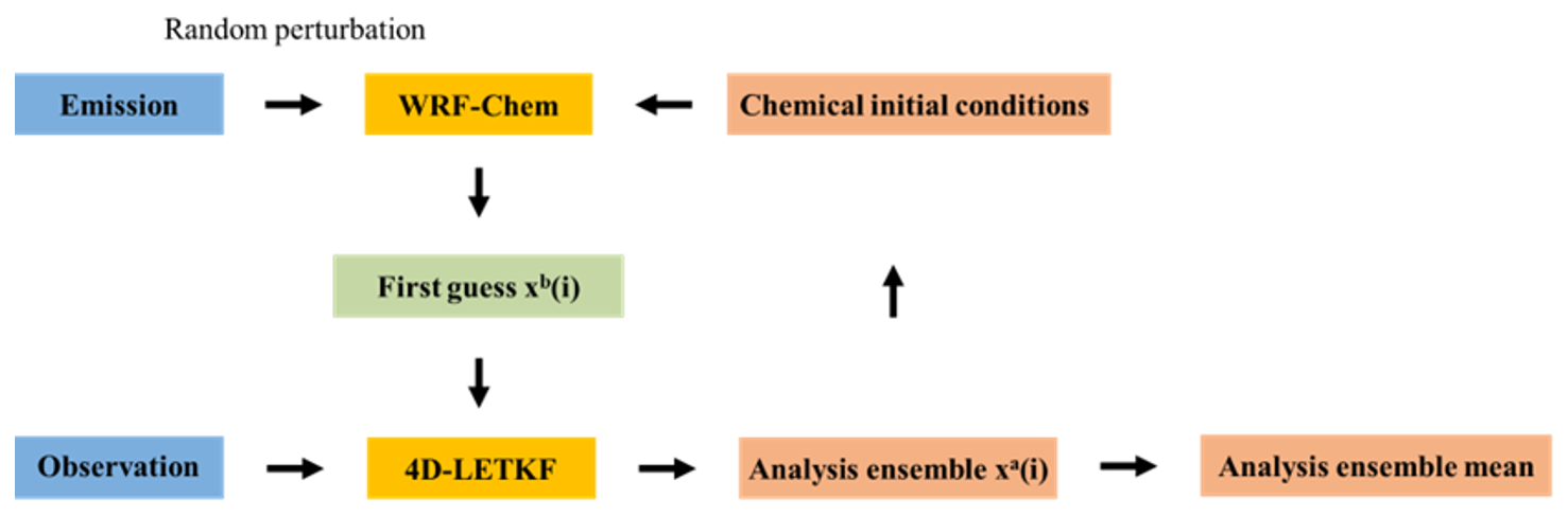
A series of control and data assimilation experiments during severe and moderate haze events, as listed in Table 2, have been carried out to achieve our major objective. The control experiments refer to numerical experiments without data assimilation. The Severe-FR experiment with a 48 h spin-up time is performed firstly to quantify the necessity of adjusting particulate matter concentration during a severe haze event. Severe-FR-24h, Severe-FR-48h, and Severe-FR-72h are accompanied by a restart every 24, 48, and 72 h, respectively, and update meteorological boundary conditions. Except Severe-FR, the rest of the experiments all have 24 h of spin-up time at the beginning of each restart or assimilation cycle. The settings of the assimilation experiment cycle time are the same as in corresponding control experiments. The detailed descriptions of experiment cycle time are shown in Fig. S1 in the Supplement. Since the effectiveness of 4D-LETKF is highly related to the ensemble member size and length of the assimilation window (Rubin et al., 2016), the sensitivity analysis is employed to investigate the influence from two parameters on assimilation effect (Kong et al., 2023). The selection of assimilation parameters for the sensitivity experiments includes 20, 40, and 60 for ensemble members and 24, 48, and 72 h for the length of the assimilation window empirically (Kong et al., 2021; Dai et al., 2021). All sensitivity experiments use identical WRF-Chem physical parameterizations, anthropogenic emissions, and random perturbations. Through the comparison between all assimilation experiments, the influence rules of 4D-LETKF assimilation have on the simulation of particulate matter in severe haze can be retrieved. Lastly, aiming to determine the applicable range of obtained influence rules above, two assimilation experiments in a moderate haze event are performed to validate whether the rules are also suitable for a less polluted environment. The reasons for the selection of parameters are described in detail in the next section.

Table 2 Design of the numerical experiments in this research.

The root mean square error (RMSE), mean error (bias), mean absolute error (MAE), and correlation coefficient are calculated in this study to evaluate the performance of each numerical experiment. The assimilation efficiency (AE) for estimating the data assimilation performance is also calculated by the following formulation (Yumimoto and Takemura, 2011):

$$\begin{array}{}\text{(12)}& \mathrm{AE}={\displaystyle \frac{{\mathrm{RMSE}}^{\mathrm{f}}-{\mathrm{RMSE}}^{\mathrm{a}}}{{\mathrm{RMSE}}^{\mathrm{f}}}}\times \mathrm{100}\mathit{\%},\end{array}$$

where RMSE^a and RMSE^f are RMSE with and without assimilation, respectively. According to the definition, if AE is positive, it means that RMSE has decreased due to the assimilation effect. When AE is equal to 1, RMSE in analysis completely disappears, and the analysis is equal to observations. The formulations of the correlation coefficient and root mean square error are shown in the Supplement.

3 Results

3.1 Comparison of the analysis with the control experiment

3.1.1 The reproduction of a severe haze event in BTH

It is essential to discuss the basic evolution of pollutants and the necessity of pollutant data assimilation in a severe haze event before conducting the assimilation experiments. The severe haze event selected in this study occurred from 00:00 15 January 2020 to 00:00 21 January 2020 (UTC). The AQI is a comprehensive indicator of overall air pollution and a criterion for severe haze events (Zhan et al., 2018; Bao et al., 2015). As a result, Fig. 3a shows the temporal variation in AQI at the six sites in the BTH region during the investigated period. The peak value of AQI mainly appeared on 18 January and then rapidly decreased on 19 and 20 January. The temporal averages of AQI have exceeded 200, with particulate matter identified as the primary pollutant. Figure 3b provides the correlation coefficients and standardized standard deviations of five parameters from Severe-FR shown against observations. Meteorological variables, including air temperature, dew point temperature, and wind speed, are well simulated when compared with PM_2.5 and PM₁₀. The correlation coefficients of meteorological factors are all larger than 0.6, while those of pollutant concentrations are all below 0.4. Therefore, when the meteorological conditions can be retrieved relatively accurately, particulate matter assimilation is the key to improving the simulative skill of pollutants.

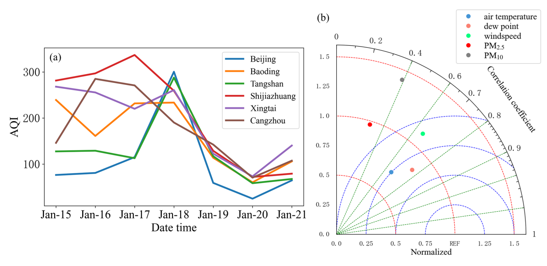
Figure 3 (a) Temporal variation about AQI at six sites in the severe haze event. (b) A Taylor graph describing the simulation from Severe-FR with five kinds of parameters compared with the observed ones in the BTH region.

3.1.2 The improvement in the reproduction of severe haze achieved by 4D-LETKF

The divergence between the assimilation and control experiments reflects the contribution from 4D-LETKF initial condition adjustment. Consequently, the study takes an ensemble member size of 40 and assimilation window length of 48 h to conduct the sensitivity experiment and compare it with Severe-FR-48h, which has the same integration time in each cycle to validate the effectiveness of the 4D-LETKF assimilation system (the analysis from the selection of 40 ensemble members and 48 h of the assimilation window length is presented here because it shows the best performance among sensitivity experiments in the next section). Figure 4 reveals the performance of control and assimilation experiments in the severe haze event. The RMSE values of PM_2.5 and PM₁₀ in Severe-FR-48h are 69.93 and 106.88 µg m⁻³, and both have a scattered distribution, indicating substantial uncertainty exists in reproducing this severe haze event. In Severe-40m-48h, the RMSE values of PM_2.5 and PM₁₀ are 31.19 and 76.83 µg m⁻³, decreasing by 55.40 % and 28.12 %, respectively, in a high-particulate-matter-concentration environment. The decreased RMSE values also imply that the assimilation system has reached a well-calibrated stage. Not only are more points grouped together, but smaller simulation errors for PM_2.5 and PM₁₀ also imply that Severe-40m-48h outperforms Severe-FR-48h in this severe haze event.

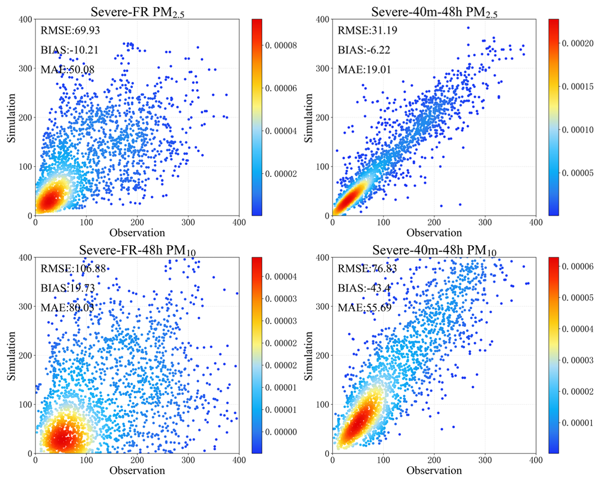
Figure 4 Scatterplot and density plot of PM_2.5 and PM₁₀ in Severe-FR-48h and Severe-40m-48h versus observations from verification stations (µg m⁻³). The color bar represents the Gaussian kernel density estimation.

In order to acquire the base distribution of simulation errors for particulate matter, Fig. 5 presents the frequency distribution of deviations between observed and simulated particulate matter concentrations in Severe-FR-48 and Severe-40m-48h experiments. It is obvious that Severe-40m-48h increases the frequency of low deviations and decreases those of high deviations in the simulation of PM_2.5. The deviation pattern of PM_2.5 in Severe-40m-48h is generally more squeezed together, with higher peaks, and symmetrical to the value of 0 than Severe-FR-48h. For the deviation distribution pattern of PM₁₀, it shows a high frequency of negative deviations and great underestimation in the Severe-FR-48h, and this underestimation has been effectively corrected by the adjustment of initial conditions and step analysis in Severe-40m-48h. In particular, the proportion of deviation within 20 µg m⁻³ in the Severe-40m-48h is 69.98 % for PM_2.5 and 31.90 % for PM₁₀.

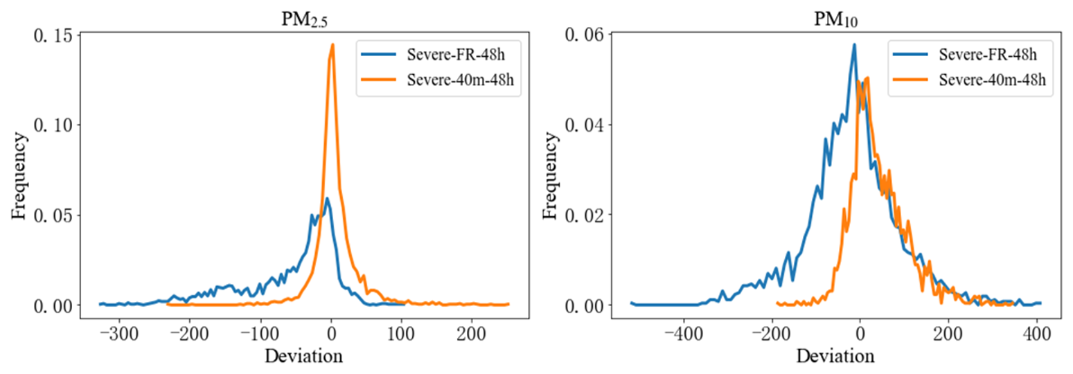
Figure 5 Frequency distribution of the deviations about the simulated PM_2.5 and PM₁₀ concentrations in Severe-40m-48h and Severe-FR-48h with the observed ones subtracted (deviation is in µg m⁻³).

Figure 6 exhibits the spatial distribution of four statistical parameters about RMSE for particulate matter in the BTH region. By comparing from the Severe-FR-48h and Severe-40m-48h, it is clear there is a significant RMSE reduction for PM_2.5 after assimilation, implying that the actual evolution of PM_2.5 can be better represented by Severe-40m-48h. For instance, the RMSE values of PM_2.5 in Baoding, Hengshui, and Cangzhou have significantly decreased to 29.85, 18.98, and 19.06 µg m⁻³, respectively, compared to 80.55, 55.22, and 76.32 µg m⁻³ in Severe-FR-48h. AE in most verification stations exceeding 50 % also suggests the high efficiency of 4D-LETKF assimilation for the simulation of PM_2.5. Although the performance of the assimilation experiment in Shijiazhuang does not have a good agreement with observation and shows a positive difference, high values of AE in most verification stations also prove the validation of the assimilating effect for PM₁₀. Compared to Severe-FR-48h, Severe-40m-48h productively reduces the RMSE of PM₁₀, accompanied by high values of 61.18 %, 59.17 %, and 52.18 % of AE on Zhangjiakou, Tangshan, and Hengshui, respectively.

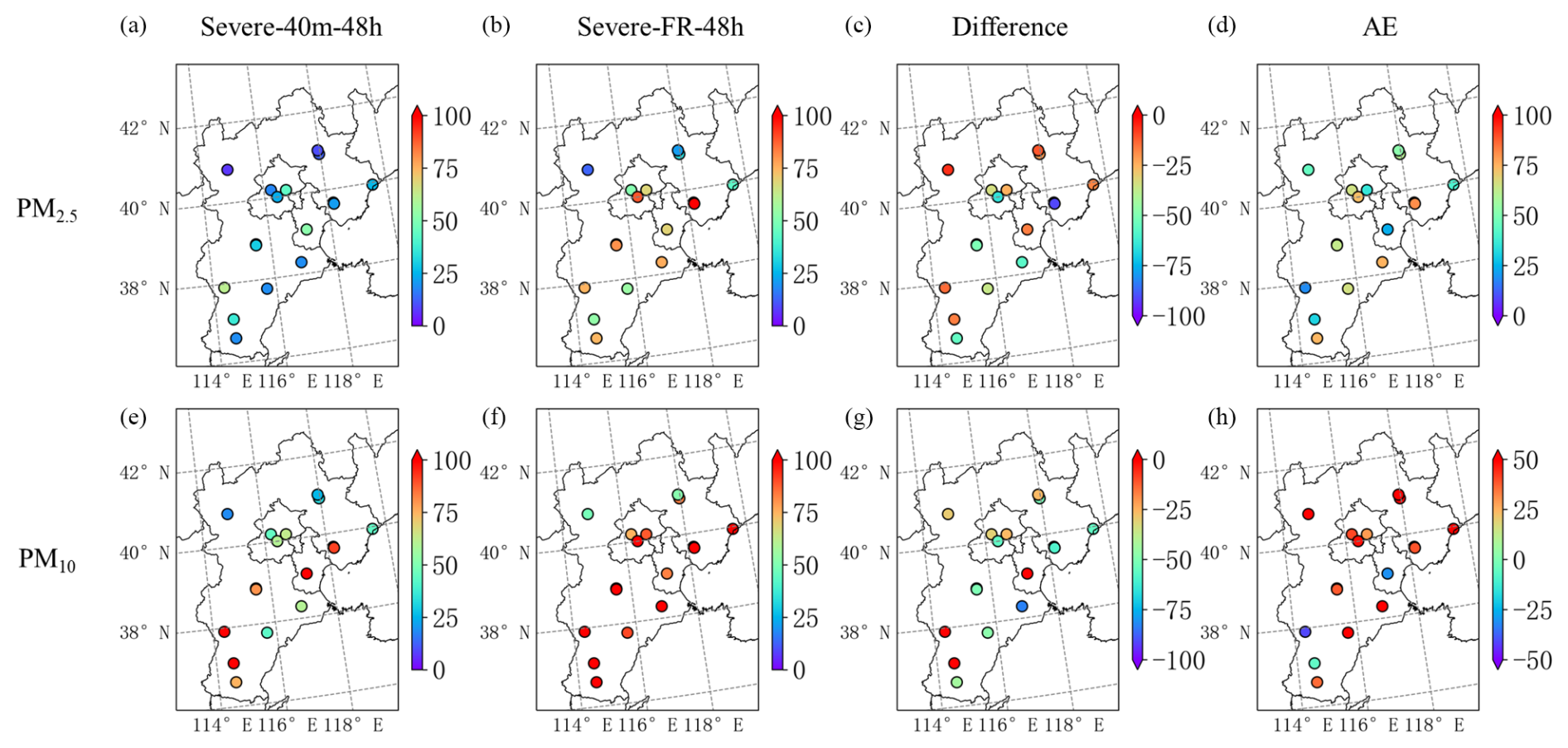
Figure 6 Spatial distribution of RMSE values from Severe-40m-48h (a, e), Severe-FR-48h (b, f), and their difference (c, g) and AE (d, h) for PM_2.5 (a–d) and PM₁₀ (e–h) from 15 to 21 January among verification stations in the BTH region. The difference implies the RMSE in Severe-40m-48h without those in Severe-FR-48h (µg m⁻³). AE is assimilation efficiency and has been described in the Methodology section. The grey border denotes the BTH region.

The spatial distribution of correlation coefficients from Severe-40m-48h, Severe-FR-48h, and their difference for PM_2.5 and PM₁₀ is also illustrated in Fig. 7. The assimilation experiment increases the correlation coefficients to more than 0.6 at all sites in the simulations of PM_2.5 and exceeds 0.7 in the southern BTH region in the simulations of PM₁₀. Severe-40m-48h also reverses the opposite trend of PM_2.5 and PM₁₀ series in Severe-FR-48h versus observations; for example, the correlation coefficients in Severe-FR-48h at Chengde and Zhangjiakou are −0.42 and −0.53, but they increase to 0.52 and 0.69 after assimilation in the simulations of PM₁₀. Incorporating more assimilable observations may further increase the correlation coefficient in the simulation of particulate matter (Kong et al., 2021). Data assimilation by multiple observations from diverse platforms is necessary because it can integrate and coordinate observational information into aerosol forecasts them well and then improve air pollutant forecast accuracy (Barbu et al., 2009; Ma et al., 2020).

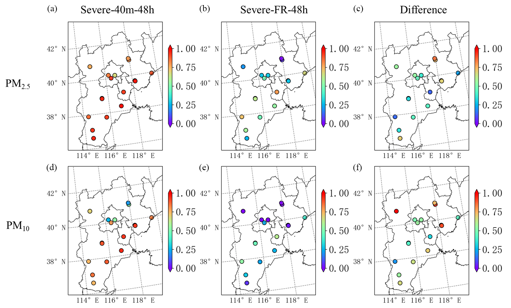
Figure 7 Spatial distribution of correlation coefficients from Severe-40m-48h (a, d), Severe-FR-48h (b, e), and their difference (c, f) for PM_2.5 (first row) and PM₁₀ (second row) from 15 to 21 January among verification stations in the BTH region. The difference implies the correlation coefficient in Severe-40m-48h without those in Severe-FR-48h. The grey border denotes the BTH region.

The temporal variations in particulate matter from Severe-40m-48h and Severe-FR-48h and observations from six independent verification stations are shown in Figs. S2 and S3. The six independent verification stations have experienced different levels of air pollution and distributed uniformly over the BTH region. It is apparent that the analysis at six stations have good agreement with observations for both PM_2.5 and PM₁₀, which can better characterize the peaks and valleys of particulate matter concentration over investigated period.

Table 3 lists the ΔRMSE, ΔCORR, and AE in the simulations of particulate matter at independent stations outside the BTH region. The RMSEs and correlation coefficients have decreased and increased, respectively, after assimilating ground-based observations, suggesting that the uncertainty in Severe-FR-48h has been well optimized in not only the BTH region, but also the whole simulation domain. The main source of these gains is generated from local initial field assimilation. Compared to Severe-FR-48h, the analysis in Yuncheng shows that the RMSE values of PM_2.5 and PM₁₀ have decreased remarkably by 98.26 and 144.56 µg m⁻³, and such a great improvement may be related to the enhanced estimation capability about state variables of particulate matter. The high values of AE also suggest that verification observation sites outside the BTH region have achieved a good Kalman gain. In previous research, predicting heavy haze events in northern China, especially over the BTH Region, remained a challenge when compared to other regions like Pearl River Delta and Yangtze River Delta in China (Feng et al., 2018; Gao et al., 2017). In this research, the analysis is propagated by meteorological elements, including temperature, air pressure, and wind fields, which come from NCEP Final analysis data and may provide an optimal meteorological boundary conditions for the assimilation of pollutant concentrations.

Table 3 Statistics about PM_2.5 and PM₁₀ from analyses in the cities among neighboring provinces of the BTH region. ΔRMSE (ΔCORR) represents the RMSE (correlation coefficient) from the analysis with those from Severe-FR-48h subtracted (ΔRMSE is in µg m⁻³).

3.2 The sensitivity of 4D-LETKF to ensemble member size and length of the assimilation window

In the previous section, the performance from the assimilation experiment with 40 ensemble members and 48 h of assimilation window length is compared against those which do not integrate hourly pollutant observations. The results fully demonstrate the ability of the 4D-LETKF assimilation method to reproduce severe haze events in spatial and temporal dimensions. However, the 4D-LETKF assimilation effect highly relies on the selection of the ensemble member size and length of the assimilation window; so how is the assimilation approach different from the parameterized selection in the severe haze event? It is of great meaning to conduct sensitivity experiments based on the ensemble member size and length of the assimilation window, compare each of their performances according to statistical metrics, and summarize the general influence rule of the 4D-LETKF parameter selection. Consequently, nine panels of sensitivity experiments are conducted with the selection of the ensemble member size (20, 40, and 60 members) and the length of the assimilation window (24, 48, and 72 h) to maximize the positive innovation in this section.

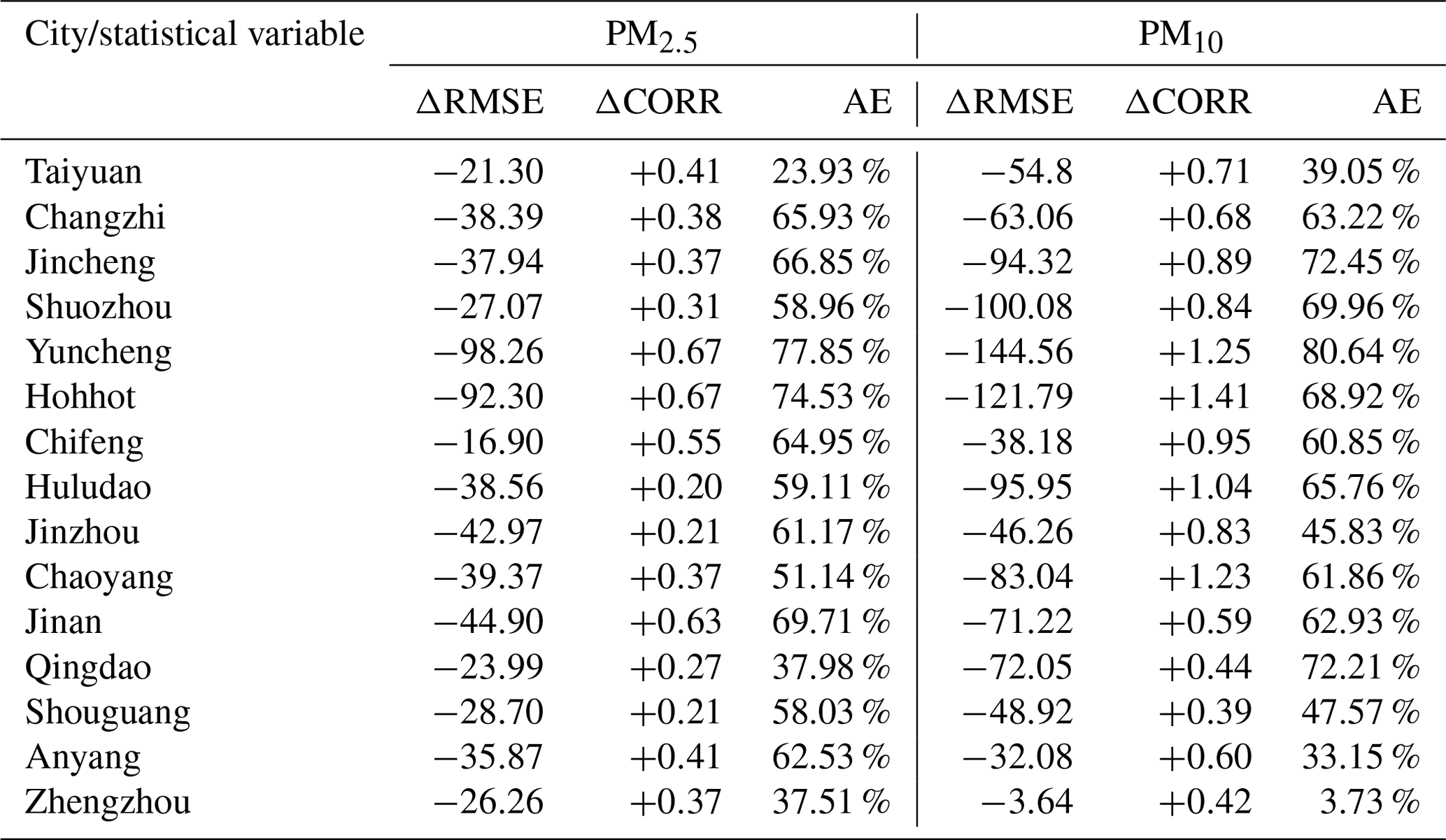
Figure 8 reveals the heatmap of RMSE in each sensitivity experiment of particulate matter over verification sites among the BTH region. The results of the free-run experiment with different integration times (24, 48, and 72 h) are offered here for comparison with analysis which have the same assimilation cycle time. The RMSEs of PM_2.5 and PM₁₀ in each free-run experiment exceed 60 and 100 µg m⁻³, respectively. It is apparent that 4D-LETKF performs better than the FR experiment in the simulation focusing on PM_2.5 and PM₁₀ over a wide range of ensemble member sizes and assimilation window lengths, illustrating the broad applicability of 4D-LETKF data assimilation to these parameters. However, it can be found that the analysis of PM_2.5 and PM₁₀ is dependent on the length of the assimilation window and dramatically related to ensemble member size in all sensitivity experiments. Unlike the short-lived and chemical reactive species (such as SO₂ and NO₂) which easily undergo complex and non-linear photochemical reactions, a relatively longer assimilation window length seems more suitable for assimilating ground-based particulate matter observations (Peng et al., 2017; Kong et al., 2021). A longer assimilation window length could also avoid the underestimation of model spread, which implies overconfidence in the first-guess state estimate by enough integration time for each member (Schutgens et al., 2010; Miyazaki et al., 2012a; Hunt et al., 2007). Hence, 48 or 72 h assimilation windows are advised to optimize the ensemble concentration trajectories. On the other hand, increasing ensemble member size efficiently reduces uncertainty in PM_2.5 and PM₁₀, as evidenced by the decrease in RMSEs from free-run to assimilation experiments with 20 and 40 members. However, when compared with the results from 40 ensemble members, the accuracy of numerical simulations does not significantly improve for PM_2.5 and PM₁₀ with 60 ensemble members either, indicating that 40 members are sufficient and feasible to provide a reliable estimation of the background error and analysis rather than more numerical source consumption. Considering numerical source consumption and RMSE values in the simulations of PM_2.5 and PM₁₀, Severe-40m-48h is more comparable to the observations when compared with the other eight panels of sensitivity experiments.

Figure 8 Heatmap showing the RMSE in each sensitivity experiment of particulate matter over verification sites (µg m⁻³). The number in each small square represents the RMSE between the observation and simulation for each combination of ensemble member sizes and the lengths of assimilation window methods.

3.3 The influence of ensemble member size on the ensemble spread

In order to explore why increasing the ensemble member size can efficiently reduce the uncertainty in the analysis of PM_2.5 and PM₁₀, as revealed in Fig. 8, this study investigates the spatial distribution of the standard deviations of PM_2.5 and PM_10–2.5 of the first guess (x^b(i)) and analysis field (x^a(i)) in terms of ensemble members. The standard deviations of ensemble members describe how the emission perturbation propagates among the forward model, and this perturbation is driven by the underlying surface pollution emission inputs and meteorological conditions. Therefore, the standard deviation in the first-guess fields quantifies the dispersion degree of the ensemble background; substantially impacts the calculation of assimilation parameters, such as ensemble state vector perturbations; and further affects the performance of particulate matter predictions.

Since the RMSE decreases with increasing ensemble member size when 20 and 40 members are in the setting, and a 48 h assimilation window corresponds to a smaller RMSE, this study compares the spatial distribution of ensemble standard deviations from Severe-20m-48h and Severe-40m-48h to explain the relationship between the ensemble member size and simulation errors in the analysis result. Figure 9 depicts contour maps of the spatial distribution of temporal averaged standard deviations in the first guess and analysis of Severe-40m-48h, Severe-20m-48h, and their difference for PM_2.5 and PM_10–2.5 during the severe haze event. The first guess in Severe-40m-48h and Severe-20m-48h shows that the relatively high standard deviations are generally observed in the southern BTH region, while those in the northern areas are close to zero for both PM_2.5 and PM_10–2.5. High-value centers are distributed in densely populated areas and urban centers including Shijiazhuang, Xingtai, Tianjin, and Tangshan, where the standard deviations generally exceed 30 µg m⁻³. Combined with Fig. S4, it can be seen that the areas with large concentration standard deviations correspond well to the spatial distribution of anthropogenic emissions and the areas with large standard deviations of emission sources. The standard deviations of concentrations of PM_2.5 and PM_10–2.5 have a close relationship with the allocation and configuration of anthropogenic emission sources because disturbances are only added to emission sources for each ensemble member without disturbing the meteorological field in this haze event. The variation in the difference in the third column entirely comes from increasing the ensemble member size. The positive difference between Severe-40m-48h and Severe-20m-48h in the first guess suggests that increasing the ensemble member size leads to greater differences among each ensemble for both PM_2.5 and PM_10–2.5 over BTH areas. The high efficiency of 4D-LETKF is strongly influenced by sufficient information spread among ensemble members, which integrate spreading out observational information to produce the analysis from the first guess (Rubin et al., 2016). As a result, the increasing ensemble member size improves divergence for each member and facilitates the state vectors of PM_2.5 and PM_10–2.5 information spread in the first guess, which means that Severe-40m-48h performs better than Severe-20m-48h in this severe haze event. The standard deviations of PM_2.5 in the analysis are generally lower than those in the first guess. Due to the localization of 4D-LETKF, that is, the ground-based observation data only optimized for the simulation grid within a certain range, square-like areas of low standard deviations appear in the analysis of PM_2.5 for both 40 and 20 ensemble members. Nearly all assimilated stations are located at the center of low-value square areas, suggesting that 4D-LETKF tunes all PM_2.5 trajectories to a small range with a low standard deviation at each slot of analysis by the assimilation of ground-based observations. For PM_10–2.5, there are no square-like areas of low standard deviations in the analysis for both 40 and 20 ensemble members, indicating that 4D-LETKF does not have an obvious limitation for PM_10–2.5 trajectories; however, the decreased standard deviations effect from 4D-LETKF is still distinct for the particulate matter because PM₁₀ consists of PM_2.5 and PM_10–2.5 in the simulation. Enlarging the ensemble member size helps improve the standard deviations of PM_2.5 and PM_10–2.5 in the analysis, while the improving magnitude of PM_2.5 is obviously smaller than PM_10–2.5. The assimilation results are not directly influenced by the increased standard deviations in analysis. Such a low increase in standard deviations (generally below 3 µg m⁻³) is unlikely to induce uncertainty in the fitting and averaging process but facilitates divergence in initial conditions between forecasting members in the next assimilation cycle. In addition, Fig. S5 depicts the spatial distribution of the standard deviation from Severe-60m-48h, Severe-20m-48h, and their difference in the first-guess and analysis fields. It can be seen that increasing the number of ensemble members generally also improves the standard deviation in the first guess and analysis over the BTH region for both PM_2.5 and PM_10–2.5. Overall, the increase in standard deviations generated by the increasing ensemble member size directly improves the information spread of ensemble members in the first-guess field and the assimilation effect of 4D-LETKF, while the positive difference in the standard deviation in the analysis favors the variances between each initial condition in the next assimilation window during the severe haze event.

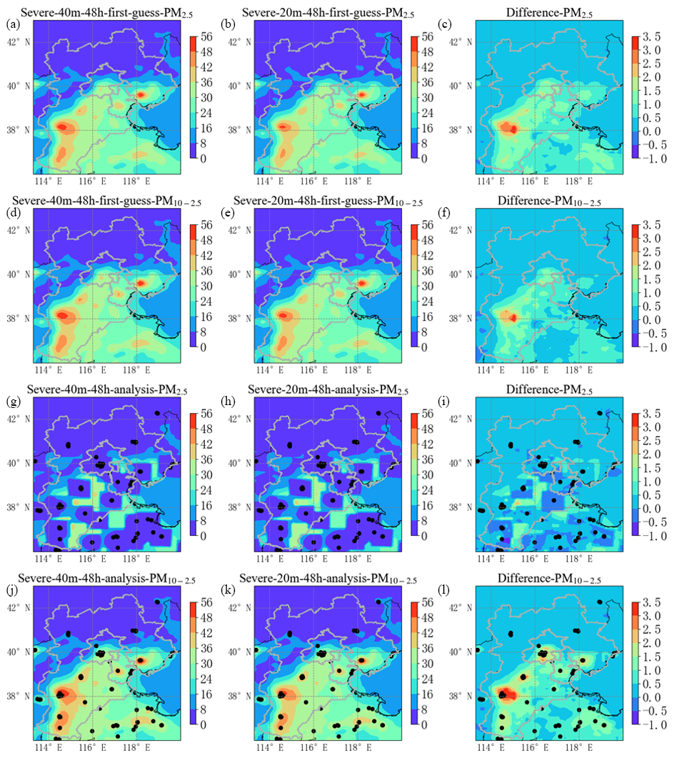
Figure 9 Contour maps of spatial distributions of temporal averaged PM_2.5 and PM_10–2.5 standard deviations in the first guess (a–f) and analysis (g–l) of Severe-40m-48h, Severe-20m-48h, and their difference (Severe-40m-48h without Severe-20m-48h) within the simulation period (µg m⁻³). The black dots in the analysis of PM_2.5 and PM_10–2.5 show the location of assimilated stations. The grey border denotes the BTH region.

On the other hand, for both the first guess from Severe-40m-48h and Severe-20m-48h, the high standard deviations are found near the Shijiazhuang region in Fig. 9, but Shijiazhuang station (37.91° N, 114.35° E) still has a larger RMSE and smaller AE, as shown in Fig. 6. This seems contrary to the opinion that increasing standard deviations in the first-guess field is beneficial to raising the accuracy of pollutant simulations. Therefore, Shijiazhuang station and the stations with high values of AE (exceed 50) and differences in the standard deviation in the first guess (exceed 1 µg m⁻³), including Beijing, Tangshan, Handan, Baoding, Cangzhou, and Hengshui regions, are selected to explore the temporal distribution of standard deviation differences between 40 and 20 ensemble members so as to further advance our understanding of the relationship between the ensemble member size and simulation uncertainty in the 4D-LETKF system. The geographical locations of observations are shown in Fig. S6 of the Supplement. Figure 10 examines the temporal distribution of the standard deviation difference for PM_2.5 and PM_10–2.5 during the investigated period at Shijiazhuang station and results averaged from the selected stations. From 17 to 18 January, the standard deviation difference in the first guess at Shijiazhuang station increased drastically and exceeded 10 µg m⁻³ for both PM_2.5 and PM_10–2.5. This uneven temporal distribution results in a large standard deviation difference of the first guess in Fig. 9. This huge divergency between ensemble members may be attributed to the peak pollutant levels with AQI exceeding 300 at Shijiazhuang station occurring on 17 January, as shown in Fig. 3. In highly polluted environments, 40 forecasting members with different perturbations in emission sources are more likely to have different concentrations of particulate matter in first-guess fields. An excessively large spread of PM_2.5 and PM_10–2.5 for ensemble members may cause an overly high estimation of background error variance and obtain a poor Kalman gain. Moreover, it can be found that the standard deviation difference in PM_2.5 and PM_10–2.5 at Shijiazhuang station is obviously lower than the average from selected stations, except for the high dispersion time, suggesting the increasing number of ensemble members has limited impact on the spread between each ensemble member at Shijiazhuang during these dates. Standard deviations that are too low imply filter divergence near Shijiazhuang station, which may induce the underestimation of model spread, reduce the effect of observation information, and make the system more certain of the state estimate of particulate matter concentrations in the first guess (Hunt et al., 2007). In addition, reducing uncertainty in the mixed anthropogenic emission inventory may be an important approach to avoid filter convergence near the Shijiazhuang region. Generally edited by empirical and statistical data such as anthropogenic emission factors and activity dataset, the anthropogenic emissions based on the bottom-up method can hardly capture the real spatiotemporal distribution of anthropogenic emissions over China as there are frequent variations in energy consumption, even in the latest version. In the southern BTH region, great positive innovations in particulate matter emissions in posterior estimation have been introduced in previous research, implying that the update of underestimated emissions in this region may enlarge ensemble spread since a large quantity of emissions corresponds to a higher degree of perturbation (Peng et al., 2017; Feng et al., 2023). In a word, the perturbations added to emissions and meteorological fields need to be executed carefully in the 4D-LETKF system to avoid too high or too low of an ensemble spread degree which determines how analysis results perform against observation information and first-guess fields (Dai et al., 2021).

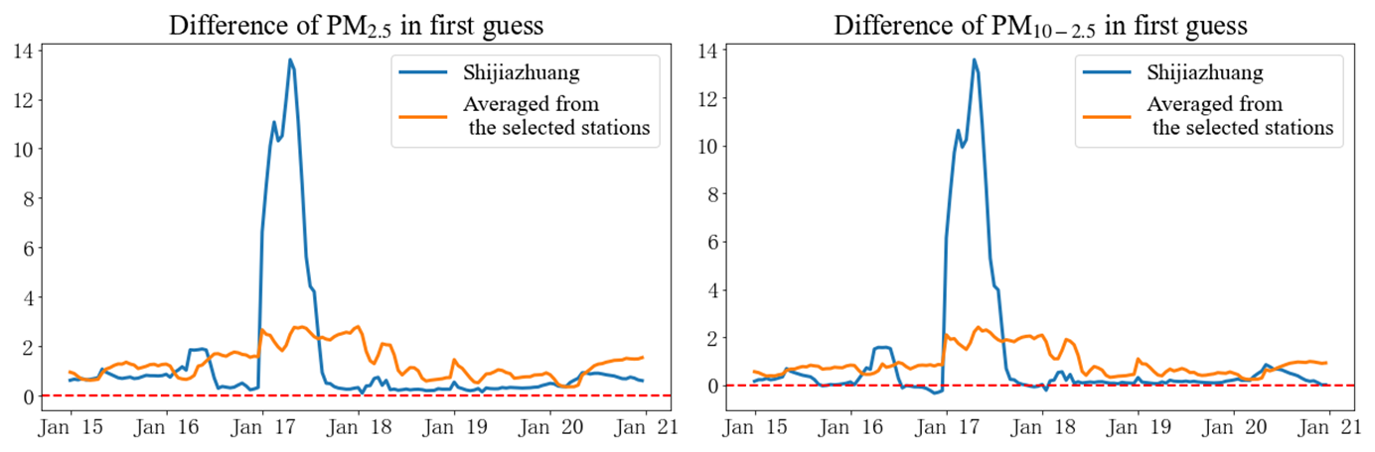
Figure 10 Temporal distribution of standard deviation difference (Severe-40m-48h without Severe-20m-48h) in the first guess for PM_2.5 and PM_10–2.5 at Shijiazhuang station, averaged from the selected stations (µg m⁻³). The dashed red line represents a value of zero.

The results above suggest that the increasing ensemble member size enlarges ensemble spread, benefits the information spread in the first guess, and finally improves the simulation skill in the severe haze event. However, it has not been determined whether these influence rules are also practical for a more common and less polluted condition. Therefore, two assimilation experiments in a moderate haze event, Moderate-20m-48h and Moderate-40m-48h, are performed to examine the applicable range. As shown in Fig. S7, the moderate haze event spans from 00:00 15 January 2019 to 00:00 21 January 2021 (UTC). This moderate event began on 15 January, with AQI increasing until 18 January, reaching a moderate level but not lasting for a long time, and then decreasing on 19 and 20 January. Most areas experienced mild or moderate air pollution, with AQI generally below 200; the primary pollutant was particulate matter after calculation. The simulations of the moderate haze event utilize the same anthropogenic emission inventory as used in the severe haze event since the two events both happen in January, thereby avoiding the additional influence introduction from emission source variation and the perturbations to the information spread and assimilation effect.

Figure S8 shows the simulated concentrations of PM_2.5 and PM₁₀ against ground-based observations during the moderate air pollution event. The RMSEs of PM_2.5 in Moderate-FR-48h, Moderate-20m-48h, and Moderate-40m-48h are 40.40, 24.12, and 18.52µg m⁻³, respectively, and the RMSEs of PM₁₀ are 73.47, 67.81, and 57.04 µg m⁻³, respectively. The concentrations of PM_2.5 and PM₁₀ in assimilation experiments are more in agreement with observations, suggesting the validation of 4D-LETKF initial condition adjustment in the moderate haze event. The phenomenon that the simulation error in PM_2.5 and PM₁₀ decreases with an increasing ensemble member size is the same as those characteristics have shown in the severe haze event before.

Similar to Fig. 9, Fig. S9 presents the spatial distributions of standard deviations of PM_2.5 and PM₁₀ in the first guess of Moderate-40m-48h, Moderate-20m-48h, and their difference. The relatively smaller magnitude of the standard deviation difference in the first guess may relate to relatively low PM_2.5 and PM₁₀ concentrations in the moderate haze event. A positive difference in the first guess and analysis for particulate matter implies the Moderate-40m-48h obtains a higher diversity of ensemble members than Moderate-20m-48h which are also similar with those happening in the severe haze event.

4 Summary

The numerical reproduction of severe haze events with an AQI larger than 200 has been a challenging problem in the field of atmospheric pollution for a long time. In this research, a WRF-Chem–4D-LETKF coupled data assimilation system has been successfully developed by an ensemble member with perturbed anthropogenic emissions to improve the simulative skill of particulate matter in the severe haze event during the winter of 2020. The research validates the effectiveness of 4D-LETKF data assimilation, discusses the optimal parameter combination of the ensemble member size and length of the assimilation window for the 4D-LETKF assimilation system, and summarizes and explains the influence rules from parametric selection to the 4D-LETKF assimilation effect during the severe and moderate haze events.

It is concluded that the Severe-40m-48h experiment shows the best performance in the simulations of PM_2.5 and PM₁₀ after comparing the statistical errors and computing resource consumption across multiple sensitivity analyses, with RMSEs of 31.19 and 76.83 µg m⁻³ for PM_2.5 and PM₁₀ in the severe haze event. Severe-40m-48h optimizes the underestimation of particulate matter concentrations in Severe-FR-48h and remarkably improves the simulation accuracy in the entire BTH region and neighboring provinces. For example, the RMSEs of PM_2.5 in Baoding, Hengshui, and Cangzhou decrease to 29.85, 18.98, and 19.06 µg m⁻³, respectively, from 80.55, 55.22, and 76.32 µg m⁻³ in Severe-FR-48h. Severe-40m-48h is also capable of retrieving the peaks and valleys of particulate matter concentration over the investigated period. To examine the dependence of the assimilation effect of 4D-LETKF, nine panels of sensitivity tests were conducted according to the ensemble member size and length of the assimilation window. The findings suggest that the simulation accuracy of PM_2.5 and PM₁₀ can be strongly improved by increasing the ensemble member size from 20 to 40. A relatively longer assimilation window length such as 48 or 72 h combined with an ensemble member size of 40 is advised in the 4D-LETKF assimilation system. In view of performance of the ensemble members, increasing ensemble member size improves ensemble spread among each forecasting member, facilitates the spread of state vectors of PM_2.5 and PM₁₀ information in the first guess, favors the variances between each initial condition in the next assimilation window, and leads to better performance in the simulation of the severe haze event. A similar conclusion can also be drawn from the moderate haze event, suggesting that this influence rule is applicable in both severe and moderate haze conditions.

There are still some deficiencies in this research. Although we have performed data quality control in this study, we do not use approaches such as super observations to improve the correspondence between grid points and observations (Jin et al., 2022; Miyazaki et al., 2012a), which may increase the representational error and result in the possibility of two stations with different concentrations interpolating on the same grid. Improving the spatial resolution of the forward model or introducing super observations may mitigate this problem (Miyazaki et al., 2012b; Feng et al., 2020b). Furthermore, the concentration of state variables of particulate matters in initial conditions is optimized in this study, but there still remain large uncertainties in anthropogenic emission data, which is important chemical boundary input for pollutant simulations. These uncertainty sources may play a significant role in the over- or underestimation of pollutant ensemble modeling. The anthropogenic emission inversion based on an ensemble Kalman filter and their variants is recognized as an effective approach to reducing uncertainty in anthropogenic emission sources (Peng et al., 2018; Feng et al., 2020a; Chen et al., 2019b). The jointly adjusted initial conditions and emission source with 4D-LETKF should be the focus of future work to further improve the forecast skills regarding air pollutants during heavy-pollution events.