Presentation, calibration and testing of the DCESS II Earth system model of intermediate complexity (version 1.0)

A new Earth system model of intermediate complexity, DCESS II, is presented that builds upon, improves and extends the Danish Center for Earth System Science (DCESS) Earth system model (DCESS I). DCESS II has considerably greater spatial resolution than DCESS I while retaining the fine, 100 m vertical resolution in the ocean. It contains modules for the atmosphere, ocean, ocean sediment, land biosphere and lithosphere and is designed to deal with global change simulations on scales of years to millions of years while using limited computational resources. Tracers of the atmospheric module are temperature, nitrous oxide, methane (^12,13C isotopes), carbon dioxide (${}^{\mathrm{12},\mathrm{13},\mathrm{14}}$C isotopes) and atmospheric oxygen. For the ocean module, tracers are conservative temperature, absolute salinity, water ¹⁸O, phosphate, dissolved inorganic carbon (${}^{\mathrm{12},\mathrm{13},\mathrm{14}}$C isotopes), alkalinity and dissolved oxygen. Furthermore, the ocean module considers simplified dynamical schemes for large-scale meridional circulation and sea ice dynamics, stratification-dependent vertical diffusion, a gravity current approach to the formation of Antarctic Bottom Water, and improvements in ocean biogeochemistry. DCESS II has two hemispheres with six zonally averaged atmospheric boxes and 12 ocean sectors distributed across the Indian–Pacific, the Atlantic, the Arctic and the Southern oceans. A new extended land biosphere scheme is implemented that considers three different vegetation types whereby net primary production depends on sunlight and atmospheric carbon dioxide. The ocean sediment and lithosphere model formulations are adopted from DCESS I but now applied to the multiple ocean and land regions of the new model.

Model calibration was carried out for the pre-industrial climate, and model steady-state solutions were compared against available modern-day observations. For the most part, calibration results agree well with observed data, including excellent agreement with ocean carbon species. This serves to demonstrate model utility for dealing with the global carbon cycle. Finally, two idealized experiments were carried out in order to explore model performance. First, we forced the model by varying Ekman transport out of the model Southern Ocean, mimicking the effect of Southern Hemisphere westerly wind variations, and second, we imposed freshwater melting pulses from the Antarctic ice sheet on the model Southern Ocean shelf. Changes in ocean circulation and in the global carbon cycle found in these experiments are in line with results from much more complex models. Thus, we find DCESS II to be a useful and computationally friendly tool for simulations of past climates as well as for future Earth system projections.

1 Introduction

The carbon cycle is the backbone of the Earth's climate system since it acts as a main regulator of global mean atmospheric temperature via atmospheric concentration of carbon dioxide (pCO₂). This cycle may be considered to be composed of two domains. One domain is a fast one with large exchange fluxes and relatively “rapid” reservoir turnovers (from years to thousands of years). This domain encompasses carbon in the atmosphere, ocean and superficial (bioturbated) ocean sediments and on land in vegetation, soil and freshwater. A second slower domain (from hundreds of thousands to millions of years) consists of huge carbon stores in rocks and sediments that exchange carbon with the fast domain through volcanic emissions of CO₂, chemical weathering, erosion and sediment formation on the seafloor. How this carbon is partitioned between the Earth's different reservoirs is what sets the pCO₂ in the atmosphere.

Earth system models (ESMs) include one or both of these domains. They are thereby useful tools that can help us gain understanding of past climates as well as make future climate projections. Depending on their complexity and spatial resolution, ESMs can take days, weeks or even months to run model simulations on the range of timescales mentioned above while using substantial computational resources. The Danish Center for Earth System Science (DCESS) model (DCESS I; Shaffer et al., 2008) is a low-order ESM with a simple geometry and ocean physics that deals with both domains of the global-scale carbon cycle and is thereby suitable for investigating Earth system changes on scales of years to millions of years while taking only minutes to days to run. The DCESS I model has proven to be a useful tool in such studies as documented by many stand-alone or intercomparison study publications (e.g., Eby et al., 2013; Harper et al., 2020; Joos et al., 2013; MacDougall et al., 2020; Shaffer, 2010; Shaffer and Lambert, 2018; Shaffer et al., 2009; Zickfeld et al., 2013). Nonetheless, DCESS I has serious limitations when it comes to addressing many important Earth system problems, like glacial–interglacial cycles, due to its one-hemisphere, two-sector horizontal resolution; lack of ocean dynamics; lack of seasonal cycles; and simplified land vegetation scheme, among other factors. In order to address those deficiencies, here we present a new Earth system model, DCESS II, that contains great improvements in model geometry and physical–biogeochemical processes. This new model is able not only to capture relevant environmental differences between major ocean basins, but also, for example, to produce synthetic ocean sediment cores from distinct ocean zones for more detailed comparison with data, and this it can do while retaining much of the simplicity and the spirit of the DCESS I model. Thus, DCESS II is a simple, fast and highly flexible ESM of intermediate complexity that is well suited to running long-term experiments in a relatively simple way with no need for substantial computational resources.

This paper is organized as follows: in Sect. 2 we describe the modules of atmosphere, ocean, ocean sediment, land biosphere and lithosphere. In Sect. 3, we present the model solution and calibration procedure and show results for the model steady-state, pre-industrial simulation. In addition, we carry out two idealized experiments in order to explore and test model performance. Finally in Sect. 4 we discuss our results, outline future perspectives and present conclusions.

2 Model description

DCESS II is an intermediate-complexity Earth system model containing atmosphere, ocean, land biosphere, lithosphere and ocean sediment modules designed to deal with global climate simulations on scales of years to millions of years. It is an enhancement and extension of the original DCESS I model (Shaffer et al., 2008) and includes, for example, a much improved horizontal and time resolution as well as simplified ocean dynamics. Model geometry consists of two hemispheres with a land–ocean area distribution and ocean depth distribution as shown in Fig. 1.

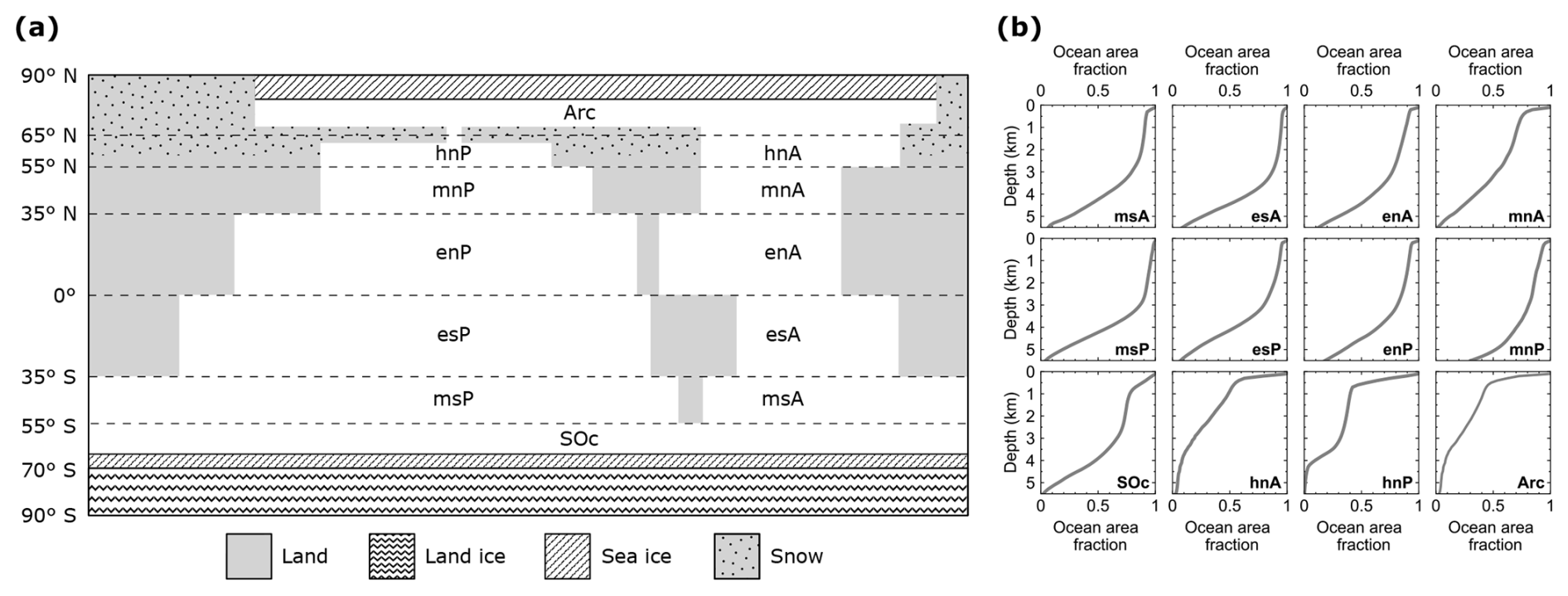
Figure 1 (a) Pre-industrial model land continental distribution and meridional boundaries of ocean sectors (dashed lines). There are 12 ocean sectors with their respective identifiers: Arc, Arctic Ocean; SOc, Southern Ocean; hn, high north; mn, mid-north; and en, equatorial north for the Atlantic (A) and Indian–Pacific (P) oceans. Sector names in the Southern Hemisphere follow the same convention. High-latitude North Pacific sector (hnP) and the Arctic Ocean are connected through the Bering Strait. Land south of 70° S is fully ice covered. Meridional sea ice and snow line extents vary freely. (b) The observed present-day ocean area fraction profile of each ocean model sector calculated from Amante and Eakins (2009).

The atmospheric module considers three zonally averaged boxes per hemisphere as low-, mid-, and high-latitude sectors divided at 35° (ϕ₃₅) and 55° (ϕ₅₅) north and south latitudes (Fig. 2a). In the ocean module we include an extra division at 65° N which allows us to consider four global ocean basins (Atlantic, Indian–Pacific, Arctic and Southern Ocean; for simplicity, hereafter the Indian–Pacific Ocean will be called only the Pacific Ocean). The Southern Ocean is 360° wide and extends up to 69° S, where it interacts with an ocean shelf extending to 70° S. In total, there are 12 ocean sectors (compared to only 2 in DCESS I). Each ocean sector is divided into 55 vertical layers with 100 m vertical resolution reaching 5500 m depth. An ocean sediment segment is assigned to each of the layers (Fig. 2b). For each sector, ocean layer and ocean sediment areas are determined from observed ocean depth distributions (Fig. 1b).

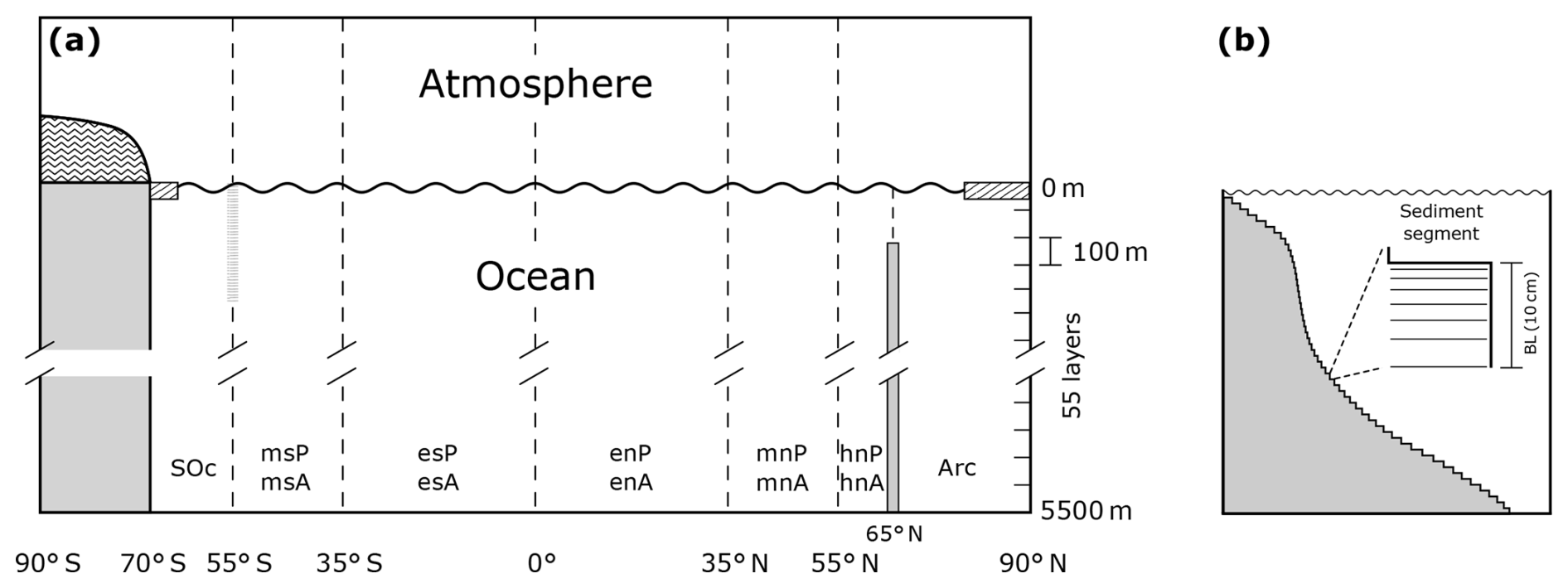
Figure 2 (a) Ocean–atmosphere cross-section view depicting meridional distributions of ocean and atmospheric boxes. There are six zonally averaged atmospheric boxes and 12 ocean sectors (see also Fig. 1a). The shaded vertical bar at 55° S extending from the surface to 2000 m depth is a virtual barrier against meridional geostrophic flow above the Drake Passage sill depth. The vertical barrier at 65° N extending from the bottom up to 1000 m depth is a physical barrier associated with Denmark Strait bathymetry. (b) Sketch of an idealized vertical area profile for an ocean sector (the actual profile for each sector is based on bathymetry observations; see Fig. 1b). Also shown is an idealized sediment segment contained in a 100 m thick box layer (the area of each specific segment is again based on bathymetric observations). The bioturbated layer (BL) is assumed to be 10 cm thick and is divided into seven sublayers as shown.

The land biosphere module considers three different types of vegetation per hemisphere whose latitudinal limits varying dynamically according to climate conditions. All model modules are described in detail in the following subsections.

2.1 Atmosphere exchange, heat balance and ice–snow extent

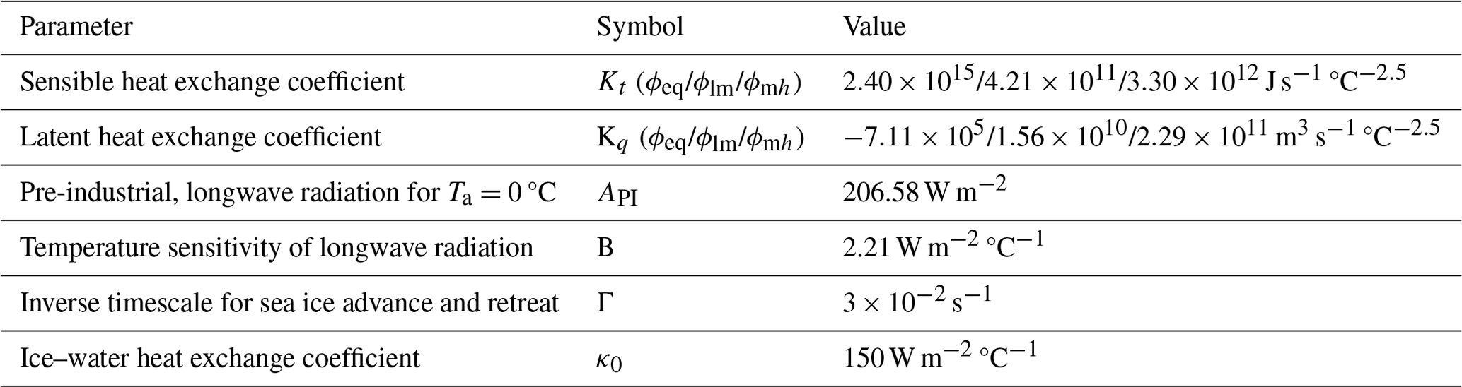
We use a simple, zonally integrated energy balance model for the near-surface atmospheric temperature, T_a (°C), forced by seasonally varying insolation, heat exchange with the ocean and meridional heat transport. In combination with simple sea ice and snow parameterizations, the model includes the ice–snow albedo feedback and the insulating effect of sea ice. Prognostic equations for mean T_a in the 0–35°, 35–55° and 55–90° zones ($T_{\mathrm{a}}^{l,m,h}$) are obtained by integrating the surface energy balance over the zones as

$$\begin{array}{}\text{(1)}& \begin{array}{rl}\mathrm{\Lambda }{\displaystyle \frac{\mathrm{d}{T}_{\mathrm{a}}^{l,m,h}}{\mathrm{d}t}}& =r^{\mathrm{2}}\underset{\mathrm{0}}{\overset{\mathrm{2}\mathit{\pi }}{\int }}\underset{\mathrm{0},{\mathit{\varphi }}_{\mathrm{35}},{\mathit{\varphi }}_{\mathrm{55}}}{\overset{{\mathit{\varphi }}_{\mathrm{35}},{\mathit{\varphi }}_{\mathrm{55}},\mathit{\pi }/\mathrm{2}}{\int }}\\ & \left(F^{\mathrm{toa}}-F^{\mathrm{T}}\right)\cos \mathit{\varphi }\mathrm{d}\mathit{\varphi }\mathrm{d}\mathit{\xi }\pm F^{\mathrm{merid}},\end{array}\end{array}$$

where $\mathrm{\Lambda }=A^{l,m,h}{\mathit{\rho }}_{\mathrm{0}}{C}_p{b}^{l,m,h}$, with $A^{l,m,h}$ denoting the atmospheric box areas, ρ₀ the reference density of water, C_p the specific heat capacity and $b^{l,m,h}$ the thicknesses chosen to yield observed seasonal cycles of $T_{\mathrm{a}}^{l,m,h}$ (partially based on Olsen et al., 2005), and r, ϕ and ξ are the Earth's radius, latitude and longitude, respectively. Furthermore, F^toa and F^T are the vertical fluxes of heat through the top of atmosphere and the ocean surface, respectively, while F^merid corresponds to the loss (equatorward box) or gain (poleward box) of heat due to meridional transport across ϕ₃₅ or ϕ₅₅. A no-flux boundary condition has been applied at the poles. At each point in time, we construct atmospheric temperature as a continuous function of latitude, T_a(ϕ), using a fourth-order Legendre polynomial in the sine of latitude ϕ,

$$\begin{array}{}\text{(2)}& T_{\mathrm{a}}\left(\mathit{\varphi }\right)=\sum T_n{P}_n\left(\sin \mathit{\varphi }\right),n=\mathrm{2},\mathrm{4},\end{array}$$

where coefficients T₀, T₂ and T₄ are determined by matching the area-weighted zone mean values of T_a(ϕ) to the prognostic mean sector values of $T_{\mathrm{a}}^{l,m,h}$ in each hemisphere. Observations show that eddy heat fluxes in the mid-latitude atmosphere are much greater than advective heat fluxes there (Oort and Peixoto, 1983). By neglecting the advective heat fluxes, Wang et al. (1999) developed suitable expressions for F^merid and the associated moisture flux, E^merid, in terms of T_a and $\partial T_{\mathrm{a}}/\partial \mathit{\varphi }$ at ϕ (for clarity we omit the index referencing low- to mid- and mid- to high-latitude boundaries, ϕ₃₅ and ϕ₅₅, respectively):

$$\begin{array}{}\text{(3)}& {\displaystyle }\begin{array}{rl}{F}^{\mathrm{merid}}& =-\left[K_t+L_v{K}_q\exp \left(-\mathrm{5420}{T}_{\mathrm{a}}^{-\mathrm{1}}\right)\right]\\ & {\left|\partial T_{\mathrm{a}}/\partial \mathit{\varphi }\right|}^{m-\mathrm{1}}\partial T_{\mathrm{a}}/\partial \mathit{\varphi },\end{array}\text{(4)}& {\displaystyle }{E}^{\mathrm{merid}}=-K_q\exp \left(-\mathrm{5420}{T}_{\mathrm{a}}^{-\mathrm{1}}\right){\left|\partial T_{\mathrm{a}}/\partial \mathit{\varphi }\right|}^{m-\mathrm{1}}\partial T_{\mathrm{a}}/\partial \mathit{\varphi },\end{array}$$

where K_t is a sensible heat exchange coefficient, K_q is a latent heat exchange coefficient and L_v is the latent heat of condensation (2.25×10⁹ J m⁻³). From observations, m is found to vary with latitude (Stone and Miller, 1980), and on this basis we take m to be 2.5 and 1.7 at ϕ₃₅ and ϕ₅₅, respectively. The temperatures and temperature gradients entered in Eqs. (3)–(4) above are obtained from Eq. (2). The poleward freshwater flux crossing a latitude ϕ is evaporated from an equatorward ocean sector and drains into the respective poleward Atlantic, Pacific, Arctic or Southern Ocean basin/sector in accordance with observed land catchment areas (Rodriguez et al., 2011). In this way, each ocean sector receives a net freshwater flux from precipitation minus evaporation. The Arctic Ocean is an exception to this in as much as a fraction of E^merid crossing 55° N also drains there, emulating large northward-flowing rivers in Canada and Siberia. Furthermore, an atmospheric zonal transport of freshwater of 0.15 Sv (1 Sv = 10⁶ m³ s⁻¹) is prescribed from the tropical North Atlantic sector to the tropical North Pacific sector, emulating the effects of trade winds there (Dey and Döös, 2020; Lohmann and Lorenz, 2000). All these fluxes force respective ocean sectors (see Sect. 2.3).

Based on a calibration procedure that makes use of monthly observed atmospheric temperature, we derived the following expression for interhemispheric heat transport at the Equator:

$$\begin{array}{}\text{(5)}& \begin{array}{rl}{F}^{\mathrm{eq}}& =K_t^{\mathrm{eq}}\partial T_{\mathrm{a}}/\partial \mathit{\varphi }+\mathrm{1.1}+\left[K_q^{\mathrm{eq}}{L}_v\partial T_{\mathrm{a}}/\partial \mathit{\varphi }-\mathrm{1.1}\right]\\ & \exp \left[-\mathrm{5420}\left(\stackrel{\mathrm{‾}}{T_{\mathrm{a}}^{{\mathrm{eq}}^{-\mathrm{1}}}}-\stackrel{\mathrm{‾}}{T_{\mathrm{a},\mathrm{PI}}^{{\mathrm{eq}}^{-\mathrm{1}}}}\right)\right],\end{array}\end{array}$$

where $K_t^{\mathrm{eq}}$ and $K_q^{\mathrm{eq}}$ are sensible and latent heat coefficients and $\stackrel{\mathrm{‾}}{T_{\mathrm{a}}^{\mathrm{eq}}}$ and $\stackrel{\mathrm{‾}}{T_{\mathrm{a},\mathrm{PI}}^{\mathrm{eq}}}$ are the model and observed pre-industrial atmospheric mean temperature at the Equator. For the ${\stackrel{\mathrm{‾}}{T}}_{\mathrm{a}}^{\mathrm{eq}}$ calculation, Eq. (2) is used and evaluated at 0° latitude for the Northern Hemisphere and Southern Hemisphere. The heat flux at the top of the atmosphere is taken as the balance between shortwave and longwave radiation as follows:

$$\begin{array}{}\text{(6)}& F^{\mathrm{toa}}=\left(\mathrm{1}-\mathit{\alpha }\right)Q-\left(A+B{T}_{\mathrm{a}}\right),\end{array}$$

where α is the planetary albedo, equal to 0.62 for ice and snow-covered areas and equal to ${\mathit{\alpha }}_{\mathrm{0}}-{\mathit{\alpha }}_{\mathrm{2}}\left(\mathrm{3}{\sin }^{\mathrm{2}}\mathit{\varphi }-\mathrm{1}\right)$ otherwise. This formulation includes the effect of mean cloud cover and lower solar inclination at higher latitudes (Hartmann, 2016), and Q is the orbitally, seasonally and latitudinally varying (and if needed, paleo-time-varying) shortwave radiation (Berger and Loutre, 1991). The albedo of areas not covered by snow/ice varies with vegetation type since forested areas have lower albedo than non-forested areas (Bonan, 2008). We adopt the approach in Eichinger et al. (2017) that includes this effect by relating the α₀ factor to the vegetation type whereby ${\mathit{\alpha }}_{\mathrm{0}}=\mathrm{0.3}-\mathit{\gamma }\left(\mathrm{1}-f\left(\mathit{\delta }{T}_{\mathrm{a}}\right)/f_{\mathrm{0}}\right)$, where the factor 0.3 is the present-day value of α₀ and γ is a multiplier equal to 0.02. f(δT_a) is the ratio between the area of grassland–savanna–desert zone and the total area not covered by snow/ice as a function of δT_a, the deviation of atmospheric temperature from the present-day value (f₀ is the ratio at δT_a=0; see Sect. 2.6 for details about vegetation zones). Finally, α₂ is equal to 0.0875.

The second term on the right-hand side of Eq. (6) is the outgoing longwave radiation (Budyko, 1969), where A and BT_a are the flux at T_a=0 and the deviation from this flux, respectively. This simple formulation implicitly includes the radiative effects of changes in cloud cover and in atmospheric water vapor content. Greenhouse gas forcing is modeled by taking A to depend on deviations of (prognostic) atmospheric partial pressures of carbon dioxide, methane and nitrous oxide (pCO₂, pCH₄ and pN₂O) from their pre-industrial values (PI) such that

$$\begin{array}{}\text{(7)}& A=A_{\mathrm{PI}}-\left(A_{{\mathrm{CO}}_{\mathrm{2}}}+A_{{\mathrm{CH}}_{\mathrm{4}}}+A_{{\mathrm{N}}_{\mathrm{2}}\mathrm{O}}\right),\end{array}$$

where expressions for $A_{{\mathrm{CO}}_{\mathrm{2}}}$, $A_{{\mathrm{CH}}_{\mathrm{4}}}$ and $A_{{\mathrm{N}}_{\mathrm{2}}\mathrm{O}}$ are taken from Byrne and Goldblatt (2014) and are valid for atmospheric concentrations in the range of 200–10 000 ppm for CO₂ and 0.1–100 ppm for CH₄ and N₂O. Overlap of the absorption by N₂O with CO₂ and CH₄ is included in these formulations. We take the year 1765 as our pre-industrial (PI) baseline, when values of pCO_2,PI, pCH_4,PI and pN₂O_PI were 280, 0.72 and 0.27 ppm, respectively, as indicated by ice-core data (IPCC, 2021, and citations therein). For simplicity and for the consideration of possible paleo-applications, we take constant values of A_PI and B for all atmospheric boxes (see Table 1). For each ocean sector, air–sea heat exchange is calculated according to Haney (1971) as

$$\begin{array}{}\text{(8)}& F^{\mathrm{T}}=-L_{\mathrm{o}}-\mathit{\lambda }\left(T_{\mathrm{a}}^{\mathrm{if}}-T_{\mathrm{o}}\right),\end{array}$$

where L_o is the direct (solar) heating of the ocean surface layer, taken to be 40, 20 and 0 W m⁻² for the low-, mid- and high-latitude sectors, respectively; λ is a constant bulk transfer coefficient, as a good approximation taken to be 30 W m⁻² °C⁻¹ but set to zero for areas covered by sea ice (Haney, 1971); $T_{\mathrm{a}}^{\mathrm{if}}$ is the ice-free mean atmospheric temperature for each sector; and T_o is the zone mean ocean surface temperature of each ocean sector.

Table 1 Atmosphere module parameters.

2.1.1 Sea ice and snow cover

Sea ice plays a pivotal role in the Earth's climate system, influencing radiative balance and thus global atmospheric temperature through its impact on surface albedo and air–sea heat exchange processes. For the sea ice cover, we take the same simple dynamical formulation as in Olsen et al. (2005) for the seasonal, equatorward sea ice extent. This formulation takes advantage of the meridional profile of T_a and assumes that (a) sea ice advance is proportional to the inverse timescale of cooling (τ^adv) of the ocean mixed layer to freezing temperature (T_f) by heat loss to the atmosphere and (b) that the retreat is proportional to the inverse timescale of melting (τ^ret) of seasonal sea ice cover. These inverse timescales are expressed as

$$\begin{array}{}\text{(9)}& {\displaystyle }{\mathit{\tau }}^{\mathrm{adv}}={\displaystyle \frac{\mathit{\lambda }}{{\mathit{\rho }}_{\mathrm{0}}{C}_p{d}_u}}{\displaystyle \frac{T_{\mathrm{a}}\left({\mathit{\varphi }}_{\mathrm{i}}\right)-T_{\mathrm{o}}}{T_{\mathrm{o}}-T_{\mathrm{f}}}},\text{(10)}& {\displaystyle }{\mathit{\tau }}^{\mathrm{ret}}={\displaystyle \frac{k_{\mathrm{i}}}{{\mathit{\delta }}_{\mathrm{i}}^{\mathrm{2}}{\mathit{\rho }}_{\mathrm{i}}{L}_{\mathrm{i}}}}\left[T_{\mathrm{a}}\left({\mathit{\varphi }}_{\mathrm{i}}\right)-T_{\mathrm{f}}\right]+{\displaystyle \frac{{\mathit{\kappa }}_{\mathrm{0}}}{{\mathit{\delta }}_{\mathrm{i}}{\mathit{\rho }}_{\mathrm{i}}{L}_{\mathrm{i}}}}\left[T_{\mathrm{o}}-T_{\mathrm{f}}\right],\end{array}$$

where d_u is the mixed-layer depth (100 m); T_a(ϕ_i) is the atmospheric temperature at the sea ice edge; T_o is the ocean surface temperature; and k_i, δ_i, ρ_i, L_i and κ₀ are the thermal conductivity of ice (2.0 W m⁻² °C⁻¹), the sea ice thickness (2 m), the density of ice (917 kg m⁻³), the latent heat of fusion of ice (3.34×10⁵ J kg⁻¹), and the heat transfer coefficient between ice and water (150 W m⁻² °C⁻¹; Bendtsen, 2002), respectively. Thus, changes in the sea ice line position are determined individually for the Arctic–North Atlantic, North Pacific and Southern Ocean as

$$\begin{array}{}\text{(11)}& {\displaystyle \frac{\partial {\mathit{\varphi }}_{\mathrm{i}}}{\partial t}}=-\mathrm{\Gamma }\left({\mathit{\tau }}^{\mathrm{adv}}-{\mathit{\tau }}^{\mathrm{ret}}\right),\end{array}$$

where Γ is a free parameter that together with κ₀ has been chosen to match the observed seasonal amplitude and the annual mean position of sea ice cover, respectively. Land areas are covered by snow where T_a(ϕ)≤0 °C and are taken to respond instantaneously to atmospheric temperature changes. Furthermore, present-day Northern Hemisphere ice sheets are prescribed as a constant area with ice albedo throughout the year independent of the snow line position. All of Antarctica is covered by ice in the model.

2.2 Atmospheric chemistry and air–sea gas exchange

For each atmospheric box we consider partial pressures of ${}^{\mathrm{12},\mathrm{13},\mathrm{14}}$CO₂, ^12,13CH₄, N₂O and O₂. The prognostic equation for the partial pressure of a gas χ is taken to be

$$\begin{array}{}\text{(12)}& {\displaystyle \frac{\mathrm{d}p\left(\mathit{\chi }\right)}{\mathrm{d}t}}={\displaystyle \frac{\mathrm{1}}{v_{\mathrm{a}}}}\left[A_{\mathrm{o}}^{\mathrm{if}}{\mathrm{\Psi }}_{\mathrm{S}}\left(\mathit{\chi }\right)+{\mathrm{\Psi }}_{\mathrm{I}}\left(\mathit{\chi }\right)\pm {\mathrm{\Psi }}_{\mathrm{T}}\left(\mathit{\chi }\right)\right],\end{array}$$

where v_a is an atmospheric mole volume; $A_{\mathrm{o}}^{\mathrm{if}}$ is an ice-free ocean surface area; Ψ_S is an air–sea gas exchange flux; Ψ_I denotes sources or sinks within the atmosphere or net transports to or from the atmosphere via weathering, volcanism, interaction with land biosphere and – for recent times – anthropogenic activities; and Ψ_T is the gas transport between adjacent atmospheric boxes.

Air–sea exchange for ¹²CO₂ for each atmospheric box is written as (for simplicity we omit the atmospheric box index superscript)

$$\begin{array}{}\text{(13)}& {\mathrm{\Psi }}_{\mathrm{S}}=k_{\mathrm{w}}{\mathit{\eta }}_{{\mathrm{CO}}_{\mathrm{2}}}\left({p\mathrm{CO}}_{\mathrm{2}}-{p\mathrm{CO}}_{\mathrm{2},\mathrm{w}}\right),\end{array}$$

where the gas transfer velocity k_w is $\mathrm{0.39}{u}^{\mathrm{2}}{\left(Sc/\mathrm{660}\right)}^{-\mathrm{0.5}}$ with u being the long-term annual mean wind speed at 10 m above the ocean surface, Sc the CO₂ Schmidt number that depends on prognostic temperatures of the ocean surface layers (Wanninkhof, 1992), and ${\mathit{\eta }}_{{\mathrm{CO}}_{\mathrm{2}}}$ the CO₂ solubility that is a function of temperature and salinity of the surface ocean layer (Weiss, 1974). pCO_2,w is the prognostic CO₂ partial pressure at the ocean surface layer equal to $\left[{\mathrm{CO}}_{\mathrm{2}}\right]/{\mathit{\eta }}_{{\mathrm{CO}}_{\mathrm{2}}}$, where [CO₂] is the prognostic dissolved CO₂ concentration of the ocean surface layer calculated from ocean carbonate carbon chemistry (see Sect. 2.4). Wind speeds are not calculated in our simplified atmosphere module, so we use observed values from the NOAA/CIRES/DOE 20th Century Reanalysis (V3) dataset for each ocean sector. For extremely warm climate experiments (annual mean sea-surface temperatures over 30 °C), we use the Schmidt number formulation from Gröger and Mikolajewicz (2011), who demonstrated that the Wanninkhof (1992) formulation underestimates Sc in such conditions.

Air–sea exchange for ⁱCO₂ (i=13 and 14) is given by

$$\begin{array}{}\text{(14)}& {\mathrm{\Psi }}_{\mathrm{S}}^i=k_{\mathrm{w}}{\mathit{\eta }}_{{\mathrm{CO}}_{\mathrm{2}}}^i{\mathit{\alpha }}_{\mathrm{k}}\left({}^i{\mathit{\alpha }}_{\mathrm{aw}}{p}^i{\mathrm{CO}}_{\mathrm{2}}-{}^i{\mathit{\alpha }}_{\mathrm{wa}}{p\mathrm{CO}}_{\mathrm{2},\mathrm{w}}{\displaystyle \frac{\left[{\mathrm{DI}}^{\mathrm{i}}\mathrm{C}\right]}{\left[\mathrm{DIC}\right]}}\right),\end{array}$$

where ⁱα_k=0.99912 is the kinetic fractionation factor (Zhang et al., 1995), [DIⁱC] and [DIC] are concentrations of dissolved inorganic carbon in the surface ocean layer, ⁱα_aw is the fractionation factor due to different solubilities in the equilibration process, and ⁱα_wa is the fractionation factor in the dissociation reactions associated with ocean carbonate chemistry. This latter term is expressed as

$$\begin{array}{}\text{(15)}& {}^i{\mathit{\alpha }}_{\mathrm{wa}}={\displaystyle \frac{\left[{\mathrm{CO}}_{\mathrm{2}}\right]+{}^i{\mathit{\alpha }}_{{\mathrm{HCO}}_{\mathrm{3}}}\left[{\mathrm{HCO}}_{\mathrm{3}}^{-}\right]+{}^i{\mathit{\alpha }}_{{\mathrm{CO}}_{\mathrm{3}}}\left[{\mathrm{CO}}_{\mathrm{3}}^{\mathrm{2}-}\right]}{\mathrm{DIC}}},\end{array}$$

where ${}^i{\mathit{\alpha }}_{{\mathrm{HCO}}_{\mathrm{3}}}$ and ${}^i{\mathit{\alpha }}_{{\mathrm{CO}}_{\mathrm{3}}}$ are individual fractionation factors for the carbon species $\left[{\mathrm{HCO}}_{\mathrm{3}}^{-}\right]$ and $\left[{\mathrm{CO}}_{\mathrm{3}}^{\mathrm{2}-}\right]$ and surface layer values for these species are obtained from ocean carbonate chemistry calculations. Moreover, ${}^i{\mathit{\alpha }}_{{\mathrm{HCO}}_{\mathrm{3}}}$ and ${}^i{\mathit{\alpha }}_{{\mathrm{CO}}_{\mathrm{3}}}$ are functions of surface layer temperature (Zhang et al., 1995). As the rate at which different isotopes of a chemical element take part in a chemical reaction depends on their mass, we assume the ${}^{\mathrm{14}}\mathrm{C}{/}^{\mathrm{12}}\mathrm{C}$ fractionation to be twice as strong as that of ${}^{\mathrm{13}}\mathrm{C}{/}^{\mathrm{12}}\mathrm{C}$, and then ${}^{\mathrm{14}}\mathit{\alpha }=\mathrm{1}-\mathrm{2}\left(\mathrm{1}{-}^{\mathrm{13}}\mathit{\alpha }\right)$.

For air–sea exchange of oxygen for each ocean surface sector,

$$\begin{array}{}\text{(16)}& {\mathrm{\Psi }}_{\mathrm{S}}=k_{\mathrm{w}}\left({\mathit{\eta }}_{{\mathrm{O}}_{\mathrm{2}}}p{\mathrm{O}}_{\mathrm{2}}-\left[{\mathrm{O}}_{\mathrm{2}}\right]\right),\end{array}$$

with k_w as before but with O₂ Schmidt numbers that depend on prognostic temperatures of the ocean surface layers (Keeling et al., 1998). The O₂ solubility (${\mathit{\eta }}_{{\mathrm{O}}_{\mathrm{2}}}$) was converted from Bunsen solubility coefficients that depend on prognostic temperatures and salinities (Weiss, 1970) to model units using the ideal gas mole volume; [O₂] is the prognostic dissolved oxygen concentration in the ocean surface layer (see Sect. 2.4). At present we do not include the air–sea exchange of methane and nitrous oxide in this model version. However, this could be readily accomplished as needed, as this has been successfully implemented in the DCESS I model (Shaffer et al., 2017).

With regard to sources and sinks (the second term on the right-hand side of Eq. 12), the model considers the following sources and sinks for each atmospheric tracer.

For carbon dioxide, there is net exchange with the land biosphere, oxidation of atmospheric methane, volcanic input, weathering of “old” organic carbon in rocks, and weathering of carbonate and silicate rocks. As needed, anthropogenic CO₂ sources associated with fossil fuel burning and/or land use change may be added. All these sources and sinks are also considered for atmospheric ¹³CO₂. For ¹⁴CO₂ the same sources and sinks as above are included, except for old (and thus ¹⁴C-free) carbon sources, which are inputs from volcanoes, organic carbon weathering and fossil fuel burning. In addition, ¹⁴C is produced naturally in the atmosphere via cosmic ray flux and, in recent times, by atomic bomb testing. For each atmospheric box, the cosmic ray source of ¹⁴CO₂ can be expressed as $A^{l,m,h}{P}_{\mathrm{14}\mathrm{C}}^{l,m,h}/A_{\mathrm{vg}}$, where A_vg is the Avogadro number and $P_{\mathrm{14}\mathrm{C}}^{l,m,h}$ (in atoms m⁻² s⁻¹) is the magnitude of ¹⁴C production, chosen here to match the estimated pre-industrial atmospheric ¹⁴C concentration such that Δ¹⁴C_atm∼0 ‰. A small amount of atmospheric ¹⁴C enters the land biosphere and decays there radioactively. A smaller fraction decays directly in the atmosphere, becoming an atmospheric sink of ¹⁴CO₂ with a decay rate λ_14C of $\mathrm{3.84}\times {\mathrm{10}}^{-\mathrm{12}}$ s⁻¹. By far most of the ¹⁴C produced enters the ocean by air–sea exchange, and by far most of this isotope decays within the ocean. Finally, a small amount of ¹⁴C enters the ocean sediment via sinking of biogenic particles and part of this returns to the ocean due to remineralization/dissolution in the ocean sediment.

For methane there is production within the land biosphere (see Sect. 2.6) and consumption associated with OH radicals in the troposphere. The latter leads to the net consumption of two O₂ molecules and production of one CO₂ molecule for every CH₄ molecule consumed. Since this reaction depletes the concentration of these radicals, the atmospheric lifetime of CH₄ grows as methane concentration rises. We include this effect in the model by taking the atmospheric methane sink to be ${\mathit{\lambda }}_{{\mathrm{CH}}_{\mathrm{4}}}p$CH₄, with ${\mathit{\lambda }}_{{\mathrm{CH}}_{\mathrm{4}}}=v_{\mathrm{a}}/{\mathit{\tau }}_{{\mathrm{CH}}_{\mathrm{4}}}$, where ${\mathit{\tau }}_{{\mathrm{CH}}_{\mathrm{4}}}$ is the (variable) atmospheric lifetime of methane. This lifetime is determined by fitting a function to the results from several modeling studies that consider a wide range of pCH₄ values. This fit yields a pre-industrial lifetime of 9.5 years, increasing for example to 10.8 and 15.1 years for 2 and 10 times the pre-industrial methane level, respectively (see Shaffer et al., 2017, for details). Potential sources like melting of methane hydrate in the Arctic tundra and ocean sediments and by human activities may be included in the model as needed. For ¹³CH₄ the same processes are considered but with their respective fractionation factors (Sect. 2.6) and adding the p¹³CH${}_{\mathrm{4}}/p^{\mathrm{12}}$CH₄ ratio to the above OH-related atmospheric methane sink formulation.

For nitrous oxide there is production within the land biosphere and consumption in the atmosphere, here mainly due to photodissociation in the stratosphere. This is modeled as ${\mathit{\lambda }}_{{\mathrm{N}}_{\mathrm{2}}\mathrm{O}}p$N₂O, with ${\mathit{\lambda }}_{{\mathrm{N}}_{\mathrm{2}}\mathrm{O}}=v_{\mathrm{a}}/{\mathit{\tau }}_{{\mathrm{N}}_{\mathrm{2}}\mathrm{O}}$, where ${\mathit{\tau }}_{{\mathrm{N}}_{\mathrm{2}}\mathrm{O}}$, the atmospheric lifetime of N₂O, is taken to be 150 years. Potential sources like N₂O flux from ocean denitrification and by human activities may be included in the model as needed.

For oxygen, there is consumption associated with oxidation of atmospheric methane and reaction with OH radicals (see above) and sinks (sources) from organic matter remineralization (photosynthesis) on land. Since methane is the end product of some of the remineralization on land (see Sect. 2.6), the land biosphere is a net O₂ source in a steady state. Furthermore, there are long-term atmospheric oxygen sinks due to weathering of organic carbon in rocks and oxidation of reduced carbon emitted in lithosphere outgassing. A long-term, quasi-steady state of pO₂ is achieved in the model when these latter sinks balance net O₂ outgassing from the ocean from less O₂ consumption than production there due to burial of organic matter in the model ocean sediments. However, for multi-million-year timescales, the global sulfur cycle would need to be included in the model to achieve “true” pO₂ steady states (Berner, 2006). Additional sinks (sources) of atmospheric O₂ associated with recent land use change and with burning of fossil fuels may be included in the model as needed.

The last term in Eq. (12) representing the gas transport between two adjacent atmospheric boxes is modeled as

$$\begin{array}{}\text{(17)}& {\mathrm{\Psi }}_{\mathrm{T}}\left(\mathit{\chi }\right)=-k_{\mathit{\chi }}{\displaystyle \frac{\mathrm{d}p\left(\mathit{\chi }\right)}{\mathrm{d}\mathit{\varphi }}},\end{array}$$

with $k_{\mathit{\chi }}=\mathrm{6}\times {\mathrm{10}}^{-\mathrm{8}}$ s⁻¹ based on data–model comparisons we made using the DCESS I model (Shaffer et al., 2008). For simplicity, we take the same value for all gases and for all atmospheric boundaries.

Evaporation and precipitation modify both salinity and oxygen isotopic composition in the surface ocean. Fractionation due to evaporation enriches (depletes) the ¹⁸O content in seawater (water vapor) from net evaporative model ocean (atmospheric) zones. Further depletion in water vapor takes place due to fractionation in the condensation process as the air mass cools in its poleward path. Given the importance of ¹⁸O in paleoclimate studies, we incorporate atmospheric cycling of oxygen isotopes of water following Olsen et al. (2005), which gives the ¹⁸O content in the well-known delta notation (δ¹⁸O_w) relative to Vienna Standard Mean Ocean Water (VSMOW). This approach takes advantage of meridional atmospheric temperature profiles estimating δ¹⁸O_a at every atmospheric box division, where the subscript “a” refers to isotopic excursion of ¹⁸O in the atmosphere.

2.3 Ocean circulation and mixing

Simplified ocean dynamics in the model consist of a balance between the pressure gradient force and linear (Rayleigh) friction acting on the meridional velocity. Model flow is defined by this relation and hydrostatic and continuity equations:

$$\begin{array}{}\text{(18)}& {\displaystyle }-{\displaystyle \frac{\mathrm{1}}{r{\mathit{\rho }}_{\mathrm{0}}}}{\displaystyle \frac{\partial P}{\partial \mathit{\varphi }}}-r_{\mathrm{f}}v=\mathrm{0},\text{(19)}& {\displaystyle }-{\displaystyle \frac{\mathrm{1}}{{\mathit{\rho }}_{\mathrm{0}}}}{\displaystyle \frac{\partial P}{\partial z}}-{\displaystyle \frac{\mathit{\rho }}{{\mathit{\rho }}_{\mathrm{0}}}}g=\mathrm{0},\text{(20)}& {\displaystyle \frac{\mathrm{1}}{r\cos \mathit{\varphi }}}{\displaystyle \frac{\partial v\cos \mathit{\varphi }}{\partial \mathit{\varphi }}}+{\displaystyle \frac{\partial w}{\partial z}}=\mathrm{0},\end{array}$$

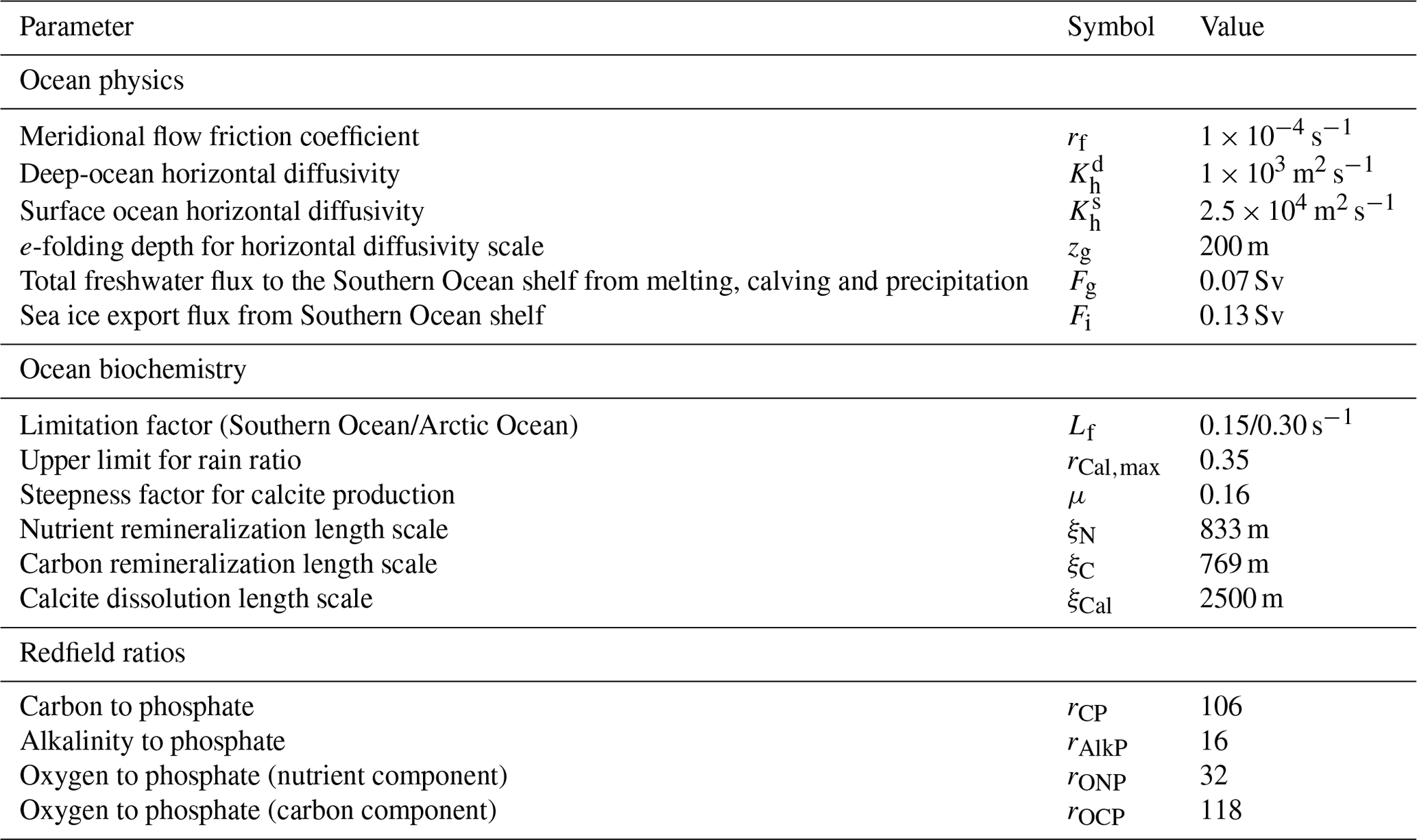
where r_f is a friction coefficient (Table 2); v and w are the meridional and vertical velocity components, respectively; P is the pressure; g is gravity; and ρ is the water density, calculated using the non-linear function of temperature, salinity and pressure according to the TEOS-10 standard (the international Thermodynamic Equation of Seawater; IOC et al., 2010) but modified for Boussinesq ocean models (Roquet et al., 2015).

Table 2 Ocean module physical and biogeochemical parameters as well as applied Redfield ratios.

Since there are no meridional boundaries at the Drake Passage, a geostrophic flow cannot be maintained above the sill depth there. To account for this feature in our simplified model, a virtual barrier against meridional flow is placed at 55° S from the surface to 2000 m depth (Fig. 2). Equatorward Ekman transport there, forced by prevailing westerly winds, is included by prescribing a net northward volume flux (E_k) in the surface layer, taken to be a total of 30 Sv injected into the South Atlantic and South Pacific sectors (msA and msP) and distributed according to the widths of these sectors. This transport, which carries Southern Ocean surface water properties, is injected into the corresponding density levels of these sectors, forming the model's Antarctic Intermediate Waters (AAIWs). Moreover, a northward surface flow of 1 Sv at 65° N is prescribed to consider the net ocean exchange between the North Pacific and the Arctic Ocean across the Bering Strait. This flow carrying surface North Pacific properties enters at the corresponding density level in the Arctic Ocean. At all other latitudes, meridional flow is set to zero in the surface layer, where exchanges rely entirely on horizontal and vertical mixing processes (Shaffer and Olsen, 2001). The zonally averaged velocity at each meridional zone boundary is related to the density field according to

$$\begin{array}{}\text{(21)}& v\left(z>d_u\right)=-{\displaystyle \frac{g}{a{r}_f{\mathit{\rho }}_{\mathrm{0}}}}\underset{\mathrm{0}}{\overset{z}{\int }}{\displaystyle \frac{\partial \mathit{\rho }}{\partial \mathit{\varphi }}}\mathrm{d}z-{\displaystyle \frac{g}{a{r}_f}}{\displaystyle \frac{\partial \mathit{\eta }}{\partial \mathit{\varphi }}},\end{array}$$

where η is the sea level and d_u is the depth of the mixed layer or, for the Southern Ocean, the Drake Passage sill depth and, for the Arctic Ocean, the Denmark Strait sill depth. Sea levels of the model ocean zones are adjusted instantaneously to conserve mass and to form sea level gradients in Eq. (21) that lead to ocean meridional transports needed to balance the Ekman transport and atmospheric freshwater forcing at the ocean surface. Finally, the vertical flow is calculated from a continuity equation, given meridional flow, Ekman transport, atmospheric freshwater forcing and shelf exchange (see below).

The effect of wind-driven gyre mixing is parameterized by a depth-dependent, horizontal diffusivity:

$$\begin{array}{}\text{(22)}& K_{\mathrm{h}}\left(z\right)=K_{\mathrm{h}}^{\mathrm{d}}+K_{\mathrm{h}}^{\mathrm{s}}\exp \left({\displaystyle \frac{z}{z_{\mathrm{g}}}}\right),\end{array}$$

where $K_{\mathrm{h}}^{\mathrm{d}}$ and $K_{\mathrm{h}}^{\mathrm{s}}$ denote the deep and surface horizontal diffusivities and z_g is an e-folding gyre depth (Table 2). At the Southern Ocean, where wind-driven gyre mixing is not important, $K_{\mathrm{h}}^{\mathrm{s}}$ is decreased by 90 %. The same approach is taken at the North Pacific sector, where North Pacific Intermediate Water (NPIW) is formed with a reduction of 50 % in $K_{\mathrm{h}}^{\mathrm{s}}$. With this setting, the model can reproduce global-scale intermediate water masses (AAIW and NPIW) in a simple way as reported by other model studies (England, 1993; Stocker et al., 1994). This is one of the few “regional tunings” in the model. The vertical diffusivity, K_v, is modeled using a stratification-dependent form, such that

$$\begin{array}{}\text{(23)}& K_{\mathrm{v}}\left(z\right)=min\left[K_{\mathrm{v}}^{\max },K_{\mathrm{v}}^{\mathrm{0}}{\left({\displaystyle \frac{N}{N_{\mathrm{0}}}}\right)}^{-\mathit{\gamma }}\right]\text{ for }N>\mathrm{0},\end{array}$$

where N is the Brunt–Väisäla frequency equal to ${\left[\left(g/{\mathit{\rho }}_{\mathrm{0}}\right)\left(\partial \mathit{\rho }/\partial z\right)\right]}^{\mathrm{1}/\mathrm{2}}$. According to Gargett and Holloway (1984), we set γ to 0.5, indicating a relatively weak dependence on stratification associated with diapycnal mixing via breaking of internal waves. Furthermore, $K_{\mathrm{v}}^{\mathrm{0}}$ and N₀ are the respective scale values of K_v and N, taken as globally representative thermocline values equal to 3 × 10⁻⁵ m² s⁻¹ and 10⁻² s⁻¹, respectively (Kunze, 2017). For unstable stratification, K_v is equated with $K_{\mathrm{v}}^{\max }$ (8 × 10⁻⁴ m² s⁻¹), accounting for model convective adjustment.

2.3.1 Southern Ocean shelf and Antarctic Bottom Water formation

Antarctic Bottom Water (AABW) constitutes a major ocean water mass filling and ventilating the abyssal ocean on a global scale (Johnson, 2008; Orsi et al., 1999). Additionally, AABW plays a crucial role through the global overturning circulation in the transport and redistribution of heat, salt, nutrients and carbon (among other tracers) and thus affects atmospheric CO₂ concentrations and thereby global climate (Orsi, 2010; Purkey and Johnson, 2013).

AABW originates from dense shelf water, formed by air cooling and brine rejection during sea ice formation, that can flow down the slope, reaching abyssal ocean depths (Gordon, 2019). To address this process, we include a 500 m deep Southern Ocean shelf (Heywood et al., 2014) between 69 and 70° S. Furthermore, we assume that there are enough air–sea heat exchanges on the shelf to maintain temperature there at freezing temperature T_f. Then the prognostic equation for all shelf tracers but temperature (ψ_sh) is

$$\begin{array}{}\text{(24)}& \begin{array}{rl}{\displaystyle \frac{\partial {\mathrm{\Psi }}_{\mathrm{sh}}}{\partial t}}& ={\displaystyle \frac{\mathrm{1}}{V_{\mathrm{sh}}}}\left[\left(F_{\mathrm{g}}-F_{\mathrm{c}}\right){\mathrm{\Psi }}_{\mathrm{g}}-F_{\mathrm{i}}{\mathrm{\Psi }}_{\mathrm{i}}\right.\\ & \left.+F_{\mathrm{r}}{\mathrm{\Psi }}_{\mathrm{SO}}-F_{\mathrm{sl},\mathrm{0}}{\mathrm{\Psi }}_{\mathrm{sh}}+F_{\mathrm{ge}}{A}_{\mathrm{sh}}^{\mathrm{if}}\right],\end{array}\end{array}$$

where V_sh is the shelf volume; F_g is the total freshwater flux to the Southern Ocean shelf from melting, calving and precipitation and F_c is the iceberg export from the shelf taken as 0.07 and 0.02 Sv, respectively. Furthermore, F_i is the sea ice export to the Southern Ocean, taken as 0.13 Sv (Haumann et al., 2016); F_r is the replacement flux from the Southern Ocean to the shelf; and F_sl,0 is the volume flux leaving the shelf at the shelf break (see below). Each of these fluxes carry their own tracer values (ψ_g, ψ_i, ψ_SO and ψ_sh). Values of Ψ_g are zero for salinity, phosphate and alkalinity tracers; ${\mathit{\eta }}_{{\mathrm{CO}}_{\mathrm{2}}}{p}^{\mathrm{12},\mathrm{13},\mathrm{14}}$CO₂ for DI${}^{\mathrm{12},\mathrm{13},\mathrm{14}}$C; ${\mathit{\eta }}_{{\mathrm{O}}_{\mathrm{2}}}$O₂ for dissolved oxygen; and a constant value of −40 ‰ for δ¹⁸O_w. The latter is a rough estimate for the mean present-day δ¹⁸O_w value of ice exported from Antarctica based on snow input values and ice sheet flow (Masson-Delmotte et al., 2008). For Ψ_i, sea ice takes the shelf water value, except for salinity, which is taken as a constant equal to 5 g kg⁻¹. Furthermore, a fraction of the freshwater flux crossing 55° S falls directly into the Southern Ocean and the rest goes to Antarctica. In a steady state, the amount going to Antarctica is equal to F_g. The last right-hand term corresponds to the air–sea gas exchange, where F_ge is the gas flux and $A_{\mathrm{sh}}^{\mathrm{if}}$ is the ice-free surface shelf area, meant mainly to represent coastal polynyas. Here we take $A_{\mathrm{sh}}^{\mathrm{if}}$ to be 20 % of the total shelf area.

If it is denser than ambient Southern Ocean water, shelf water flows down along the continental slope. On a path to the deep ocean, downslope flow takes up ambient water via entrainment, typically increasing its volume to more than twice its value at the shelf break to finally fill the abyssal ocean as AABW (Orsi et al., 2002; Orsi et al., 2001). In order to include a comparable AABW formation process in our model, we address this using a simple formulation of entrainment following approaches described in Baines (2005, 2008). The governing equations for the downslope flux (F_sl) and the plume height (or thickness, H) normal to the slope are

$$\begin{array}{}\text{(25)}& {\displaystyle \frac{\mathrm{d}{F}_{\mathrm{sl}}}{\mathrm{d}s}}=E{\displaystyle \frac{F_{\mathrm{sl}}}{H}},\text{(26)}& {\displaystyle \frac{\mathrm{d}H}{\mathrm{d}s}}=\mathrm{2}E+C_{\mathrm{d}}-S_{\mathrm{2}}Ri\tan \mathit{\theta },\end{array}$$

where s is the downslope distance from the shelf break depth obtained from observed bathymetry (Amante and Eakins, 2009) and E is the entrainment coefficient equal to $E_{\mathrm{0}}\left(\mathrm{1}-Ri/R{i}_{\mathrm{c}}\right)$ for $\le Ri\le R{i}_c$ and zero otherwise. Here Ri is the Richardson number, Ri_c is a critical value for Ri, and E₀ is an amplitude parameter. Ri is defined as $G{H}^{\mathrm{3}}\cos \mathit{\theta }/F_{\mathrm{sl}}^{\mathrm{2}}$, where $G=g\mathrm{\Delta }\mathit{\rho }\left(z\right)/{\mathit{\rho }}_{\mathrm{0}}$ is the buoyancy, Δρ(z) is the difference between downflow density and the mean local ambient density, and θ is the slope angle. Values for Ri_c and E₀ are taken to be 0.25 and 0.20, respectively (Xu et al., 2006). Finally, C_d and S₂ are the drag coefficient and a constant, respectively, with values taken from the literature cited above. Initial conditions at the shelf break are taken to be H₀=100 m and $F_{\mathrm{sl},\mathrm{0}}=H_{\mathrm{0}}{\left(G_{\mathrm{0}}{H}_{\mathrm{0}}\right)}^{\mathrm{0.5}}$, with G₀ calculated as above using the Southern Ocean density at the shelf break depth. We integrate Eqs. (25) and (26) every 2 m from the shelf break until the depth where the plume and the ambient water buoyancy are close enough as defined by a threshold. Then this downslope flow enters Southern Ocean model layers in accordance with the plume height. Although other overflow approaches have been proposed (Danabasoglu et al., 2010; Xu et al., 2006), we think that this simple and fast approach is well suited to capturing the formation and insertion of AABW at depth and is a particular strength in our simplified model. In this context we note that quite a few CMIP6 models form AABW incorrectly by deep, open-ocean convection and/or by lack of plume entrainment (Heuzé, 2021).

With the above physics and for any ocean zone, the general conservation equation of any ocean tracer ψ may be written as

$$\begin{array}{}\text{(27)}& \begin{array}{rl}{\displaystyle \frac{\partial \mathit{\psi }}{\partial t}}& +{\displaystyle \frac{\mathrm{1}}{a\cos \mathit{\varphi }}}{\displaystyle \frac{\partial \left(\cos \mathit{\varphi }v\mathit{\psi }\right)}{\partial \mathit{\varphi }}}+{\displaystyle \frac{\partial \left(w\mathit{\psi }\right)}{\partial z}}={\displaystyle \frac{\mathrm{1}}{a^{\mathrm{2}}\cos \mathit{\varphi }}}\\ & {\displaystyle \frac{\partial }{\partial \mathit{\varphi }}}\left(\cos \mathit{\varphi }{K}_{\mathrm{h}}{\displaystyle \frac{\partial \mathit{\psi }}{\partial \mathit{\varphi }}}\right)+{\displaystyle \frac{\partial }{\partial z}}\left(K_{\mathrm{v}}{\displaystyle \frac{\partial \mathit{\psi }}{\partial z}}\right)+{\mathrm{\Psi }}_{\mathrm{S}}\left(\mathit{\psi }\right)\\ & +{\mathrm{\Psi }}_{\mathrm{B}}\left(\mathit{\psi }\right)+{\mathrm{\Psi }}_{\mathrm{I}}\left(\mathit{\psi }\right),\end{array}\end{array}$$

where Ψ_S is the air–sea exchange of heat and gases, Ψ_B is the exchange of dissolved substances with the ocean sediment, and Ψ_I are internal sources and sinks into the water column. Ocean tracers of temperature, salinity and δ¹⁸O_w are forced only at the ocean surface via air–sea heat exchange and direct solar forcing for temperature and freshwater forcing for salinity and δ¹⁸O_w. Pacific Ocean and Atlantic Ocean model sectors between 35 and 55° S south of Africa are connected via a zonal surface-intensified mixing scheme in order to emulate the role of the Antarctic Circumpolar Current there. These specific terms are added to Eq. (27) for tracers of these sectors (msA and msP).

2.4 Ocean biogeochemical cycling

The ocean module considers the following biogeochemical ocean tracers: phosphate (PO₄), dissolved oxygen (O₂), dissolved inorganic carbon (DIC) in ${}^{\mathrm{12},\mathrm{13},\mathrm{14}}$C species and alkalinity (ALK), which are all forced by new (export) production of organic matter and biogenic calcium carbonate shells in the lighted ocean surface layers. Furthermore, PO₄, DI${}^{\mathrm{12},\mathrm{13},\mathrm{14}}$C and ALK are forced by river inputs and concentration/dilution of the surface layer by evaporation/precipitation. Moreover, O₂ and DI${}^{\mathrm{12},\mathrm{13},\mathrm{14}}$C are forced by air–sea exchange. In the ocean interior, all these tracers are influenced by remineralization of organic matter and dissolution of CaCO₃ shells in the water column as well as exchange with the ocean sediment. DI¹⁴C is affected by radioactive decay in all ocean layers. For simplicity, we have neglected explicit nitrogen cycling and have assumed that all biogenic matter export from the surface layer is in the form of particulate organic matter (POM) and that all CaCO₃ is in the form of calcite.

We take new (export) production of organic matter (NP) in each model surface layer to be a function of phosphorus (Maier-Reimer, 1993; Yamanaka and Tajika, 1996) and solar radiation as

$$\begin{array}{}\text{(28)}& \mathrm{NP}=A_{\mathrm{o}}^{\mathrm{if}}{z}_{\mathrm{eu}}{L}_{\mathrm{f}}\left[{\mathrm{PO}}_{\mathrm{4}}\right]{\displaystyle \frac{I}{I+I_{\mathrm{1}/\mathrm{2}}}}{\displaystyle \frac{\left[{\mathrm{PO}}_{\mathrm{4}}\right]}{\left[{\mathrm{PO}}_{\mathrm{4}}\right]+P_{\mathrm{1}/\mathrm{2}}}},\end{array}$$

where $A_{\mathrm{o}}^{\mathrm{if}}$ is the ice-free ocean surface area; z_eu is the euphotic layer depth (100 m); and [PO₄] and I are phosphate content and solar radiation in the surface ocean, respectively. $P_{\mathrm{1}/\mathrm{2}}$ and $I_{\mathrm{1}/\mathrm{2}}$ are their respective half-saturation constants equal to 1 µmol m⁻³ for phosphate and 100 W m⁻² for light (Mutshinda et al., 2017). L_f is an efficiency coefficient (units of s⁻¹) that estimates iron and/or other limitation factors on net primary production. We take the value of L_f to be equal to 1 for most ocean zones but set to some lower value for the Southern and Arctic oceans as determined by the model fit to ocean data (Sect. 3.1.2). In the surface layer, sources and sinks due to new production for PO₄, DI¹²C, ALK and O₂ are −NP, −r_CPNP, r_AlkPNP and (r_OCP+r_ONP)NP, respectively, where r_CP, r_AlkP, r_OCP and r_ONP are the Redfield ratios of C:P, ALK:P, (O₂)_C : P and (O₂)_N : P, respectively. The subscripts C and N refer to a division of POM into “carbon” and “nutrient” parts, respectively, as explained below. We adopted the Redfield ratios used in Shaffer et al. (2008) and shown in Table 2. For DI^13,14C, the surface sink due to new production and associated isotope fractionation is ${-}^{\mathrm{13},\mathrm{14}}{\mathit{\alpha }}_{\mathrm{Org}}{\left(\left[{\mathrm{DI}}^{\mathrm{13},\mathrm{14}}\mathrm{C}\right]/\left[{\mathrm{DI}}^{\mathrm{12}}\mathrm{C}\right]\right)}_{\mathrm{eu}}{r}_{\mathrm{CP}}\mathrm{NP}$. We take the fractionation factor ¹³α_Org to depend on surface ocean concentrations of dissolved carbon dioxide ([CO_2(aq)]) and phosphate according to Pagani et al. (1999):

$$\begin{array}{}\text{(29)}& {}^{\mathrm{13}}{\mathit{\alpha }}_{\mathrm{Org}}=\mathrm{25}-{\displaystyle \frac{\mathrm{116.96}{L}_{\mathrm{f}}\left[{\mathrm{PO}}_{\mathrm{4}}\right]+\mathrm{81.42}}{\left[{\mathrm{CO}}_{\mathrm{2}\left(\mathrm{aq}\right)}\right]}},\end{array}$$

where concentrations are in µmol kg⁻¹. As previously, ${}^{\mathrm{14}}{\mathit{\alpha }}_{\mathrm{Org}}=\mathrm{1}-\mathrm{2}\left(\mathrm{1}-{}^{\mathrm{13}}{\mathit{\alpha }}_{\mathrm{Org}}\right)$.

The surface (export) production of biogenic calcite is related to new (export) production by r_CalCr_CPNP, where r_CalC is the “rain” ratio, the ratio between the production of CaCO₃ and the production of organic carbon. It is parameterized according to Maier-Reimer (1993) and Marchal et al. (1998) but with the addition of a dependence on the calcite saturation state of the ocean surface layer (Ω_S) following Shaffer et al. (2016):

$$\begin{array}{}\text{(30)}& r_{\mathrm{CalC}}=r_{\mathrm{Cal},\max }{\displaystyle \frac{\exp \left(\mathit{\mu }\left(T_{\mathrm{s}}-T_{\mathrm{ref}}\right)\right)}{\mathrm{1}+\exp \left(\mathit{\mu }\left(T_{\mathrm{s}}-T_{\mathrm{ref}}\right)\right)}}{\displaystyle \frac{{\mathrm{\Omega }}_{\mathrm{S}}-\mathrm{1}}{\mathit{\nu }+\left({\mathrm{\Omega }}_{\mathrm{S}}-\mathrm{1}\right)}},\end{array}$$

where r_Cal,max is a rain ratio upper limit; μ is the steepness factor; T_s and T_ref are the surface temperature and the reference temperature (10 °C), respectively; and ν is a half-saturation constant taken to be 1 (Gangstø et al., 2011). Furthermore, ${\mathrm{\Omega }}_{\mathrm{S}}=\left[{\mathrm{Ca}}^{\mathrm{2}+}\right]\left[{\mathrm{CO}}_{\mathrm{3}}^{\mathrm{2}-}\right]/K_{\mathrm{sp}}$, with calcium concentration given as $\left[{\mathrm{Ca}}^{\mathrm{2}+}\right]={\left[{\mathrm{Ca}}^{\mathrm{2}+}\right]}_{\mathrm{m}}\left(S/S_{\mathrm{m}}\right)$, where ${\left[{\mathrm{Ca}}^{\mathrm{2}+}\right]}_{\mathrm{m}}$ and S_m are the global ocean mean calcium and salinity values, taken as 10.57 mol m⁻³ and 35 for the present day, respectively; S is the ocean salinity; and K_sp is the calcite solubility coefficient. There is no biogenic calcite production for subsaturated conditions (r_CalC=0 for Ω_S≤1). Values for r_Cal,max and μ are determined by the model fit to ocean and ocean sediment data. With this, surface sinks for DI¹²C and ALK due to biogenic calcite production are −r_CalCr_CPNP and −2r_CalCr_CPNP, respectively. For DI^13,14C, the surface sinks due to calcite production and associated isotope fractionation are ${-}^{\mathrm{13},\mathrm{14}}{\mathit{\alpha }}_{\mathrm{Cal}}{\left(\left[{\mathrm{DI}}^{\mathrm{13},\mathrm{14}}\mathrm{C}\right]/\left[{\mathrm{DI}}^{\mathrm{12}}\mathrm{C}\right]\right)}_{\mathrm{eu}}{r}_{\mathrm{CalC}}{r}_{\mathrm{CP}}\mathrm{NP}$, where α_Cal=1, assuming no carbon fractionation during biogenic calcite formation in the ocean surface layer.

Particles are assumed to sink out of the surface layer with settling speeds high enough to neglect advection and diffusion of them. This particulate flux decreases significantly with depth due to subsurface remineralization/dissolution, with only a small fraction reaching the seafloor, as shown by sediment trap data (Martin et al., 1987). To address this, we assume an exponential-type law for the vertical fraction of the particulate organic matter (POM) nutrient and carbon components, each with a distinct e-folding length (ξ_N and ξ_C) motivated mainly by results of Shaffer et al. (1999). Additionally, we also include temperature dependence (λ_Q) on remineralization rates as indicated by ocean data (Laufkotter et al., 2017; Marsay et al., 2015). Therefore, tracer sources in the water column due to the remineralization of POM, the nutrient (Φ_N) and carbon component (Φ_C), are expressed as the vertical gradient of POM:

$$\begin{array}{}\text{(31)}& {\mathrm{\Phi }}_{\mathrm{N},\mathrm{C}}\left(z\right)={\displaystyle \frac{\partial \mathrm{POM}{\left(z\right)}_{\mathrm{N},\mathrm{C}}}{\partial z}}=\mathrm{POM}{\left(z\right)}_{\mathrm{N},\mathrm{C}}{\displaystyle \frac{{\mathit{\lambda }}_Q\left(T_{\mathrm{o}}\left(z\right)\right)}{{\mathit{\xi }}_{\mathrm{N},\mathrm{C}}}},\end{array}$$

where λ_Q is defined as $Q_{\mathrm{10}}^{\left(T_{\mathrm{o}}\left(z\right)-T_{\mathrm{o},\mathrm{ref}}\right)/\mathrm{10}}$, with Q₁₀ being the biotic activity increase for a 10 °C increase in T_o, T_o,ref a reference temperature taken as the present-day global area-weighted mean observed temperature from the World Ocean Atlas 2018 database (Boyer et al., 2018) for the upper 500 m (Komar and Zeebe, 2021) and ξ_N,C e-folding lengths for $T_{\mathrm{o}}\left(z\right)=T_{\mathrm{o},\mathrm{ref}}=\mathrm{9.3}$ °C. For the biogenic calcium carbonate particle flux (PCal), we take a simple exponential law with a constant e-folding length ξ_Cal, and, as above, tracer sources in the water column due to dissolution of CaCO₃ produced in the euphotic zone (Φ_Cal) are expressed as

$$\begin{array}{}\text{(32)}& {\mathrm{\Phi }}_{\mathrm{Cal}}\left(z\right)={\displaystyle \frac{\partial \mathrm{PCal}\left(z\right)}{\partial z}}={\displaystyle \frac{\mathrm{PCal}\left(z\right)}{{\mathit{\xi }}_{\mathrm{Cal}}}}.\end{array}$$

In Eqs. (31) and (32), POM_N, POM_C and PCal at z=0 are the respective surface layer export productions, NP, r_CPNP and r_CalCr_CPNP. Given the range of Q₁₀ values shown by data and modeling studies (Laufkotter et al., 2017; Regaudie-de-Gioux and Duarte, 2012; Bendtsen et al., 2015) and to maintain model simplicity (see Sect. 2.6 and 2.7), we choose a constant value for Q₁₀ of 2. Also for simplicity, ξ_N, ξ_C and ξ_Cal are taken to be constants for all ocean zones, whose values (Table 2) have been chosen to fit ocean data (Sect. 3.1.2). Thus, the vertical source and sinks in the ocean interior for PO₄, DI¹²C, ALK and O₂ are Φ_N, (Φ_C+Φ_Cal), (2 Φ_Cal−r_AlkPΦ_N) and (r_ONPΦ_N+r_OCP Φ_C), respectively. For DI^13,14C, the vertical distribution from remineralization and dissolution is ${\left(\left[{\mathrm{DI}}^{\mathrm{13},\mathrm{14}}\mathrm{C}\right]/\left[{\mathrm{DI}}^{\mathrm{12}}\mathrm{C}\right]\right)}_{\mathrm{eu}}\left[{}^{\mathrm{13},\mathrm{14}}{\mathit{\alpha }}_{\mathrm{Org}}{\mathrm{\Phi }}_{\mathrm{C}}{+}^{\mathrm{13},\mathrm{14}}{\mathit{\alpha }}_{\mathrm{Cal}}{\mathrm{\Phi }}_{\mathrm{Cal}}\right]$. All these vertical distributions are weighted by the ocean area profile A_o(z) for each zone. In addition, the fluxes of P and ${}^{\mathrm{12},\mathrm{13},\mathrm{14}}$C that fall in the form of POM and/or biogenic calcite particles on the model ocean sediment surface at any depth of each zone are calculated as the product of $\mathrm{d}{A}_{\mathrm{o}}\left(z\right)/\mathrm{d}z$ there and the difference between the particulate fluxes falling out of the ocean surface layer and the remineralization/dissolution taking place down to the depth of each zone.

Non-linear ocean carbonate chemistry is calculated using the recursive formulation of Antoine and Morel (1995) as explained in detail in Shaffer et al. (2008) in the context of a DCESS-model approach. This system yields ocean distributions of CO_2(aq), ${\mathrm{CO}}_{\mathrm{3}}^{\mathrm{2}-}$, ${\mathrm{HCO}}_{\mathrm{3}}^{-}$ and hydrogen ion concentrations needed for calculations of air–sea exchange of carbon dioxide, carbon isotopic fractionation during air–sea exchange and ocean new production, dissolution of calcite in the ocean sediment, and pH (seawater scale). Profiles of carbonate saturation with respect to calcite are calculated as $K_{{\mathrm{CaCO}}_{\mathrm{3}}}^{\prime }/\left(\right[{\mathrm{Ca}}^{\mathrm{2}+}{]}_{\mathrm{m}}S/S_{\mathrm{m}}$), where $K_{{\mathrm{CaCO}}_{\mathrm{3}}}^{\prime }$ is the apparent dissociation constant for calcite as function of T, S and pressure (Mucci, 1983).

2.5 Ocean sediment

For the sediment module, we adopt the approach developed by Shaffer et al. (2008), the main features of which are summarized below.

Each model ocean layer of 100 m thickness is assigned a sediment segment composed of calcite, non-calcite mineral (NCM) and reactive organic matter. The segment is a bioturbated layer (BL) that is assumed to be 10 cm thick divided into seven sublayers with the highest resolution near the sediment surface such that sublayer boundaries are 0, 0.2, 0.5, 1, 1.8, 3.2, 6 and 10 cm. Sediment segment areas are determined by model topography from each ocean zone. POM and PCal rain fluxes and ocean values of T, S, DIC, ALK, O₂ and PO₄ are taken from respective layers from ocean and ocean biogeochemistry modules. NCM fluxes (F_NCM) are parameterized as

$$\begin{array}{}\text{(33)}& F_{\mathrm{NCM}}=\mathrm{NCF}\left[\mathrm{1}+\mathrm{CAF}\exp \left(-z/{\mathit{\lambda }}_{\mathrm{slope}}\right)\right],\end{array}$$

where NCF is the open-ocean non-calcite flux, CAF is an amplification factor at the coast (i.e., at z=0) and λ_slope is the e-folding water depth scale representing the effect of distance from the coast associated with continental slope topography. For simplicity, we apply the same values of NCF, CAF and λ_slope, taken to be 0.3 g cm⁻² kyr⁻¹, 20 and 200 m, respectively, to all ocean sectors.

The sediment module is designed to address calcium carbonate (CaCO₃) dissolution and (oxic and anoxic) organic matter remineralization by calculating concentrations of reactive organic carbon (OrgC), pore-water O₂ and pore-water ${\mathrm{CO}}_{\mathrm{3}}^{\mathrm{2}-}$ for each sediment sublayer. To accomplish this, a key property is the sediment porosity (ϕ_S, not to be confused with the latitude symbol), which is parameterized as a function of the calcite dry-weight fraction, (CaCO₃)_dwf:

$$\begin{array}{}\text{(34)}& {\mathit{\varphi }}_{\mathrm{S}}\left(\mathit{\zeta }\right)={\mathit{\varphi }}_{\mathrm{S},\min }+\left(\mathrm{1}-{\mathit{\varphi }}_{\mathrm{S},\min }\right)\exp \left(-\mathit{\zeta }/\mathit{\alpha }\right),\end{array}$$

where ζ is the sediment vertical coordinate, ${\mathit{\varphi }}_{\left(\mathrm{S},\min \right)}=\mathrm{1}-\left(\mathrm{0.483}+\mathrm{0.45}{\left({\mathrm{CaCO}}_{\mathrm{3}}\right)}_{\mathrm{dwf}}\right)$ and $\mathit{\alpha }=\mathrm{0.25}{\left({\mathrm{CaCO}}_{\mathrm{3}}\right)}_{\mathrm{dwf}}+\mathrm{3}\left(\mathrm{1}-{\left({\mathrm{CaCO}}_{\mathrm{3}}\right)}_{\mathrm{dwf}}\right)$ following Archer (1996). From sediment porosity, the sediment formation factor ($F_{\mathrm{S}}={\mathit{\varphi }}_{\mathrm{S}}^{-\mathrm{3}}$) is determined in order to calculate bulk sediment diffusion coefficients of pore-water solutes.

To account for the role of benthic fauna, the bioturbation rate (D_b) is parameterized not only to depend on organic carbon rain rates but also to consider attenuation associated with very low dissolved oxygen concentrations. This is formulated as

$$\begin{array}{}\text{(35)}& D_{\mathrm{b}}=D_{\mathrm{b}}^{\mathrm{0}}{\left({\displaystyle \frac{F_{\mathrm{OrgC}}}{F_{\mathrm{OrgC}}^{\mathrm{0}}}}\right)}^{\mathrm{0.85}}{\displaystyle \frac{\left[{\mathrm{O}}_{\mathrm{2},\mathrm{ocean}}\right]}{\left[{\mathrm{O}}_{\mathrm{2},\mathrm{ocean}}\right]+{\mathrm{O}}_{\mathrm{2},\mathrm{low}}}},\end{array}$$

where [O_2,ocean] is the ocean O₂ concentration at the sediment surface and O_2,low is taken to be 20 mmol m⁻³. Moreover, $D_{\mathrm{b}}^{\mathrm{0}}$ and $F_{\mathrm{OrgC}}^{\mathrm{0}}$ are the bioturbation rate scale and the organic carbon rain rate scale, whose values are 1.38 × 10⁻⁸ cm² s⁻¹ and 1 × 10⁻¹² mol cm⁻² s⁻¹, based in part on Archer et al. (2002).

Oxygen remineralization rates in the BL are taken to scale as bioturbation rates (and thereby as organic carbon rain rates; Archer et al., 2002), such as ${\mathit{\lambda }}_{\mathrm{ox}}={\mathit{\lambda }}_{\mathrm{ox}}^{\mathrm{0}}{D}_{\mathrm{b}}/D_{\mathrm{b}}^{\mathrm{0}}$. Anoxic remineralization rates in the BL are slower than oxic rates and will depend upon the specific remineralization reactions involved (e.g., denitrification is faster than sulfate reduction). More organic rain would be associated with a more anoxic BL and a shift toward sulfate reduction. Therefore, we take λ_anox=βλ_ox, where β is taken to decrease for an increasing organic carbon rain rate such that $\mathit{\beta }={\mathit{\beta }}_{\mathrm{0}}{\left(F_{\mathrm{OrgC}}/F_{\mathrm{OrgC}}^{\mathrm{0}}\right)}^{\mathit{\gamma }}$. As described in Shaffer et al. (2008), values for ${\mathit{\lambda }}_{\mathrm{ox}}^{\mathrm{0}}$, β₀ and γ were constrained by organic carbon burial observations to be 1 × 10⁻⁹ s⁻¹, 0.1 and −0.3, respectively.

Governing equations for OrgC, pore-water O₂, and ${\mathrm{CO}}_{\mathrm{3}}^{\mathrm{2}-}$ and CaCO₃ are second-order, non-linear coupled differential equations which are solved for each sediment segment using a semi-analytical iterative approach (steady state) or time-stepping approach (time dependent) by imposing boundary conditions at the top and bottom of the BL and matching conditions at the sublayer boundaries. For simplicity we also apply the same calculated sediment remineralization rates to organic phosphorus raining on the sediment surface. Using a mass balance approach, sedimentation velocity is determined and used to calculate burial rates of phosphorus, organic carbon and carbonate carbon down and out of the base of the BL. In this way the model produces synthetic sediment cores at every depth for each of the model ocean basins. Furthermore, model solutions provide fluxes between ocean and sediment layers of PO₄, O₂, DIC and ALK based on concentrations of these tracers in each respective adjacent ocean layer and sediment pore-water concentrations from organic matter remineralization and calcium carbonate dissolution. A detailed description of the sediment module is given in Appendix A of Shaffer et al. (2008).

2.6 Land biosphere

Eichinger et al. (2017) defined three different dynamically varying vegetation zones to extend and improve the original DCESS I one-zone land biosphere module. The vegetation zones – a grassland–desert zone bordered equatorward and poleward by tropical forest and extratropical forest zones, respectively – were formulated by emulating the behavior of a complex land biosphere model (Gerber et al., 2004). With this approach, latitudinal boundaries of the zones could be defined as functions of global mean temperature alone, encompassing implicit dependency on precipitation. In this way, the very different carbon distributions between, say, aboveground biomass and soil for each zone and the responses of these carbon reservoirs to changing climate and atmospheric CO₂ could be addressed. For example, while most of the carbon in tropical forests is found above the ground, by far most of the carbon in extratropical forests is in the soil (Chapin et al., 2011). With this new three-zone module, the size and timing of carbon exchanges between atmosphere and land were represented much more realistically in cooling and warming experiments than with the original one-zone module (Eichinger et al., 2017). Furthermore, our three-zone approach allows for changing biosphere modulation of radiative forcing since albedo is higher for grasslands–deserts than for forests (see albedo formulations in Sect. 2.1).

Here we use the same approach but now expanded to two hemispheres. The vegetation zones are tropical forest (TF); grassland, savanna and desert (GSD); and extratropical forest (ET), which includes carbon reservoirs for leaves (M_G), wood (M_W), litter (M_D) and soil (M_S) (Shaffer et al., 2008). Latitudinal boundaries of each vegetation zone (ϕ_TF-GSD for the TF–GSD boundary and ϕ_GSD-ET for the GSD–ET boundary) are obtained using a fifth-order polynomial dependent on the deviation of hemispheric annual mean atmospheric temperature from the respective pre-industrial temperature such that $\mathit{\varphi }\left(\mathit{\delta }{T}_{\mathrm{a}}\right)=c_{\mathrm{1}}\mathit{\delta }{T}_{\mathrm{a}}^{\mathrm{5}}+c_{\mathrm{2}}\mathit{\delta }{T}_{\mathrm{a}}^{\mathrm{4}}+c_{\mathrm{3}}\mathit{\delta }{T}_{\mathrm{a}}^{\mathrm{3}}+c_{\mathrm{4}}\mathit{\delta }{T}_{\mathrm{a}}^{\mathrm{2}}+c_{\mathrm{5}}\mathit{\delta }{T}_{\mathrm{a}}^{\mathrm{1}}+c_{\mathrm{6}}$, with $\mathit{\delta }{T}_{\mathrm{a}}=\stackrel{\mathrm{‾}}{T_{\mathrm{a}}}-\stackrel{\mathrm{‾}}{T_{\mathrm{a},\mathrm{PI}}}$. Polynomial coefficients are obtained by fitting data from Gerber et al. (2004) for the Northern Hemisphere and Southern Hemisphere separately (Table 3). Poleward ET limits are the annual mean snow line for the Northern Hemisphere and the fixed position at 55° S for Southern Hemisphere (there is no land south of 55° S; see Fig. 1a). We note that the above approach is only strictly valid for −10 °C < δT_a < 10 °C, the range considered in the original experiments of Gerber et al. (2004). For warming, this corresponds to annual mean temperatures of less than about 25 °C and corresponding atmospheric pCO₂ levels of less than about 1000–1500 ppm. For more extreme warming situations in the distant past or future, a re-evaluation of our land biosphere module would be necessary for use in model simulations.

Table 3 Coefficients for vegetation meridional limits, ϕ(δT_a), for the Northern Hemisphere and Southern Hemisphere and the global pre-industrial distribution of carbon storage and net primary production for all vegetation zones considered in the model.

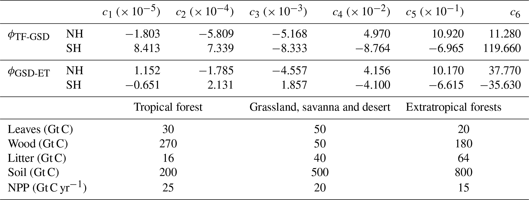
Net primary production on land (NPP) takes up atmospheric CO₂ and is forced by seasonally varying solar radiation. For each vegetation type zone, NPP is calculated according to

$$\begin{array}{}\text{(36)}& \mathrm{NPP}={\mathrm{NPP}}_{\mathrm{PI}}{A}_{\mathrm{f}}f\left(I\right)\left[\mathrm{1}+f_{{\mathrm{CO}}_{\mathrm{2}}}\ln \left({\displaystyle \frac{{p\mathrm{CO}}_{\mathrm{2}}}{{p\mathrm{CO}}_{\mathrm{2},\mathrm{PI}}}}\right)\right],\end{array}$$

where NPP_PI is the pre-industrial net primary production (see Table 3); A_f is an area factor accounting for vegetation size change with respect to pre-industrial size; $f_{{\mathrm{CO}}_{\mathrm{2}}}$ is the CO₂ fertilization factor equal to 0.37, a suitable value for the terrestrial biosphere (Eby et al., 2013; Zickfeld et al., 2013); pCO₂ is the model-calculated partial pressure of atmospheric carbon dioxide; and $f\left(I\right)=f_{\mathrm{0}}+a\exp \left(-{\left(\left(I-b\right)/c\right)}^{\mathrm{2}}\right)$ is a function fitted from model results (Hazarika et al., 2005) with coefficients a, b and c chosen to represent the seasonal cycle of solar radiation according to the specific orbital forcing parameters and f₀ chosen so that the annual mean value of f(I) for each zone is equal to 1. Note that each vegetation type has its own function f(I) with its respective parameters. With this formulation, NPP responds in a seasonal cycle according to f(I) and to atmospheric carbon dioxide on longer timescales.

With the descriptions above and the assumptions that NPP is distributed between leaves and wood at the fixed ratio of 35:25, all leaf loss goes to litter, wood loss is divided between litter and soil at the fixed ratio of 20:5, and litter loss is divided between the atmosphere (as CO₂) and the soil at the fixed ratio of 45:10 (Siegenthaler and Oeschger, 1987; Shaffer et al., 2008), the conservation equations for the land biosphere reservoirs of ¹²C for leaves (M_G), wood (M_W), litter (M_D) and soil (M_S) for each of the six vegetation zones are

$$\begin{array}{}\text{(37)}& {\displaystyle \frac{\mathrm{d}{M}_{\mathrm{G}}}{\mathrm{d}t}}={\displaystyle \frac{\mathrm{35}}{\mathrm{60}}}\mathrm{NPP}-{\displaystyle \frac{\mathrm{35}}{\mathrm{60}}}{\mathrm{NPP}}_{\mathrm{PI}}{\displaystyle \frac{M_{\mathrm{G}}}{M_{\mathrm{G},\mathrm{PI}}}},\text{(38)}& {\displaystyle \frac{\mathrm{d}{M}_{\mathrm{W}}}{\mathrm{d}t}}={\displaystyle \frac{\mathrm{25}}{\mathrm{60}}}\mathrm{NPP}-{\displaystyle \frac{\mathrm{25}}{\mathrm{60}}}{\mathrm{NPP}}_{\mathrm{PI}}{\displaystyle \frac{M_{\mathrm{W}}}{M_{W,\mathrm{PI}}}},\text{(39)}& {\displaystyle }\begin{array}{rl}{\displaystyle \frac{\mathrm{d}{M}_{\mathrm{D}}}{\mathrm{d}t}}& ={\displaystyle \frac{\mathrm{35}}{\mathrm{60}}}{\mathrm{NPP}}_{\mathrm{PI}}{\displaystyle \frac{M_{\mathrm{G}}}{M_{\mathrm{G},\mathrm{PI}}}}+{\displaystyle \frac{\mathrm{20}}{\mathrm{60}}}{\mathrm{NPP}}_{\mathrm{PI}}{\displaystyle \frac{M_{\mathrm{W}}}{M_{\mathrm{W},\mathrm{PI}}}}\\ & -{\displaystyle \frac{\mathrm{55}}{\mathrm{60}}}{\mathrm{NPP}}_{\mathrm{PI}}{\displaystyle \frac{M_{\mathrm{D}}}{M_{\mathrm{D},\mathrm{PI}}}}{\mathit{\lambda }}_Q,\end{array}\text{(40)}& {\displaystyle }\begin{array}{rl}{\displaystyle \frac{\mathrm{d}{M}_{\mathrm{S}}}{\mathrm{d}t}}& ={\displaystyle \frac{\mathrm{5}}{\mathrm{60}}}{\mathrm{NPP}}_{\mathrm{PI}}{\displaystyle \frac{M_{\mathrm{W}}}{M_{\mathrm{W},\mathrm{PI}}}}+{\displaystyle \frac{\mathrm{10}}{\mathrm{60}}}{\mathrm{NPP}}_{\mathrm{PI}}{\displaystyle \frac{M_{\mathrm{D}}}{M_{\mathrm{D},\mathrm{PI}}}}{\mathit{\lambda }}_Q\\ & -{\displaystyle \frac{\mathrm{15}}{\mathrm{60}}}{\mathrm{NPP}}_{\mathrm{PI}}{\displaystyle \frac{M_{\mathrm{S}}}{M_{\mathrm{S},\mathrm{PI}}}}{\mathit{\lambda }}_Q,\end{array}\end{array}$$

where M_G, M_W, M_D, M_S and M_PI are the pre-industrial reservoir sizes (Table 3) and ${\mathit{\lambda }}_Q=Q_{\mathrm{10}}^{\left(T_{\mathrm{a}}-T_{\mathrm{a},\mathrm{PI}}\right)/\mathrm{10}}$ with Q₁₀=2 as above (Sect. 2.4). Atmosphere–land biosphere carbon dioxide flux from each vegetation zone is

$$\begin{array}{}\text{(41)}& F_{{\mathrm{CO}}_{\mathrm{2}}}=-\mathrm{NPP}+{\mathrm{NPP}}_{\mathrm{PI}}\left[{\displaystyle \frac{\mathrm{45}}{\mathrm{60}}}{\displaystyle \frac{M_{\mathrm{D}}}{M_{\mathrm{D},\mathrm{PI}}}}+{\displaystyle \frac{\mathrm{15}}{\mathrm{60}}}{\displaystyle \frac{M_{\mathrm{S}}}{M_{\mathrm{S},\mathrm{PI}}}}\right]{\mathit{\lambda }}_Q.\end{array}$$

For isotopes ¹³C and ¹⁴C, Eqs. (37)–(41) are extended considering fractionation factors for photosynthesis and, for ¹⁴C, radioactive decay as described in Shaffer et al. (2008).

Finally, land biosphere methane and nitrous oxide productions ($F_{{\mathrm{CH}}_{\mathrm{4}}}$ and $F_{{\mathrm{N}}_{\mathrm{2}}\mathrm{O}}$, respectively) take place in soil and are proportional to the reservoir size and temperature dependent according to λ_Q, where again Q₁₀=2 for both. In addition, we assume methane emissions only from wet areas (zones TF and ET). Thus, for each vegetation zone, fluxes of these two greenhouse gases are given as

$$\begin{array}{}\text{(42)}& F_{{\mathrm{CH}}_{\mathrm{4}}}\mathrm{|}{\mathrm{N}}_{\mathrm{2}}\mathrm{O}={\mathit{\tau }}_{{\mathrm{CH}}_{\mathrm{4}}}\mathrm{|}{\mathrm{N}}_{\mathrm{2}}\mathrm{O},\mathrm{PI}{\left(p{\mathrm{CH}}_{\mathrm{4}}\mathrm{|}p{\mathrm{N}}_{\mathrm{2}}\mathrm{O}\right)}_{\mathrm{PI}}{\displaystyle \frac{M_{\mathrm{S}}}{M_{\mathrm{S},\mathrm{PI}}}}{\mathit{\lambda }}_Q,\end{array}$$

where ${\mathit{\tau }}_{{\mathrm{CH}}_{\mathrm{4}}}\mathrm{|}{\mathrm{N}}_{\mathrm{2}}\mathrm{O},\mathrm{PI}$ is the pre-industrial atmospheric lifetime of CH₄ and N₂O (9.5 and 150 years, respectively). Fluxes of ^13,14CH₄ are ${}^{\mathrm{13},\mathrm{14}}{\mathit{\alpha }}_{\mathrm{M}}{F}_{{\mathrm{CH}}_{\mathrm{4}}},\mathrm{PI}\left(M_{\mathrm{S}}^{\mathrm{13},\mathrm{14}}/M_{\mathrm{S},\mathrm{PI}}\right){\mathit{\lambda }}_Q$, with ¹³α_M=0.97 being the fractionation factor for CH₄ production. As above, we assume the ${}^{\mathrm{14}}\mathrm{C}{/}^{\mathrm{12}}\mathrm{C}$ fractionation to be twice as strong as that for ${}^{\mathrm{13}}\mathrm{C}{/}^{\mathrm{12}}\mathrm{C}$ (see Sect. 2.2). Fluxes to specific atmospheric boxes are equal to the biosphere fluxes within the latitudinal boundaries of the boxes.

2.7 Lithosphere module (rock weathering, volcanism and river input)

We follow the same approach as in the DCESS I model (Sect. 2.7 in Shaffer et al., 2008) by considering river inputs of phosphorus and carbon species, climate-dependent carbonate and silicate weathering rates, and lithosphere outgassing. However here we extend this approach to consider distributions of continents, river mouths (Dai and Trenberth, 2002) and volcanoes (NCEI Volcano Locations Database). In the following, we restrict ourselves to presenting the main features of this module (see Shaffer et al., 2008, again for more details).

Weathering rates of rocks containing phosphorus (W_P), as well as carbonate and silicate weathering rates (W_Sil and W_Cal), are taken to depend on the deviation of mean atmospheric temperature from its pre-industrial value in the form

$$\begin{array}{}\text{(43)}& \begin{array}{rl}{W}_{\mathrm{P}\mathrm{|}\mathrm{Sil}\mathrm{|}\mathrm{Cal}}& ={\mathit{\lambda }}_Q{W}_{\mathrm{P}\mathrm{|}\mathrm{Sil}\mathrm{|}\mathrm{Cal},\mathrm{PI}}\\ & =Q_{\mathrm{10}}^{\left(T_{\mathrm{a}}-T_{\mathrm{a},\mathrm{PI}}\right)/\mathrm{10}}{W}_{\mathrm{P}\mathrm{|}\mathrm{Sil}\mathrm{|}\mathrm{Cal},\mathrm{PI}},\end{array}\end{array}$$

where W_P|Sil|Cal,PI represents the pre-industrial weathering rates for phosphorus, silicate and carbonate and Q₁₀=2 as for the other model components. Vegetation affects weathering rates by modifying surface pH through the production of CO₂ or organic acids or by altering the physical properties of soil such as erosion of exposed mineral areas and by water cycling content (Drever, 1994; Berner, 1995). Our model does not explicitly include these and other factors like a direct dependency of atmospheric pCO₂ levels (Krissansen-Totton and Catling, 2017). Such factors would add extra tuneable complexity and be beyond the scope and balance of our simplified model. Silicate weathering consumes 2 mol of atmospheric CO₂ per mole of silicate mineral weathered, while the carbonate weathering consumes only 1 mol of atmospheric CO₂ per mole of carbonate mineral weathered. Both types of weathering supply bicarbonate ion to ocean surface layers, modifying dissolved inorganic carbon and alkalinity concentrations. The phosphorus supply is equal to W_P. Therefore, expressions for total river inputs for PO₄, DIC and ALK tracers are

$$\begin{array}{}\text{(44)}& {\displaystyle }{R}_{\mathrm{P}}=W_{\mathrm{P}}={\mathit{\lambda }}_Q{W}_{\mathrm{P},\mathrm{PI}},\text{(45)}& {\displaystyle }{R}_{\mathrm{DIC}}=\mathrm{2}\left(W_{\mathrm{Sil}}+W_{\mathrm{Cal}}\right)=\mathrm{2}{\mathit{\lambda }}_Q\left(W_{\mathrm{Sil},\mathrm{PI}}+W_{\mathrm{Cal},\mathrm{PI}}\right),\text{(46)}& {\displaystyle }\begin{array}{rl}{R}_{\mathrm{ALK}}& =\mathrm{2}\left(W_{\mathrm{Sil}}+W_{\mathrm{Cal}}\right)-r_{\mathrm{ALKP}}{W}_{\mathrm{P}}\\ & ={\mathit{\lambda }}_Q\left[\mathrm{2}\left(W_{\mathrm{Sil},\mathrm{PI}}+W_{\mathrm{Cal},\mathrm{PI}}\right)-r_{\mathrm{ALKP}}{W}_{\mathrm{P},\mathrm{PI}}\right].\end{array}\end{array}$$

Values of W_P,PI, W_Cal,PI and W_Sil,PI are obtained from the assumed pre-industrial steady state equal to the global ocean burial rate of phosphate (B_OrgP) and carbonate (B_Cal) and the assumption that W_Sil,PI can be taken to be a fixed ratio of carbonate weathering: $W_{\mathrm{Sil},\mathrm{PI}}={\mathit{\gamma }}_{\mathrm{Sil}}{W}_{\mathrm{Cal},\mathrm{PI}}$, with γ_Sil=0.85. These total river inputs are distributed among the 12 ocean sectors according to the river mouth distributions mentioned above. For example, this leads to no river input to the model Southern Ocean sector.

Sources of carbon to the atmosphere are weathering of rocks containing old organic carbon (W_OrgC) and lithosphere outgassing (Vol). As above, $W_{\mathrm{OrgC}}={\mathit{\lambda }}_Q{W}_{\mathrm{OrgC},\mathrm{PI}}$, and Vol may either be taken as a constant and equal to its pre-industrial value (Vol_PI) or be prescribed as an external forcing of the Earth system. Given the above together with assigned or calculated ¹³C content for the different model inputs and outputs (including for example for organic carbon burial), overall steady-state conservation equations can be formulated for both ¹²C and ¹³C. These conservation equations can then be used to derive expressions for W_OrgC,PI and Vol_PI as given in Shaffer et al. (2008) (their Eqs. 41 and 42). These total atmospheric carbon inputs are distributed among the six atmosphere sectors according to the same meridional distribution as carbonate and silicate weathering and volcano distribution mentioned above.

From the above, the pre-industrial steady-state equations for phosphorus, ¹²C and ¹³C are given by

$$\begin{array}{}\text{(47)}& {\displaystyle }{W}_{\mathrm{P}}-B_{\mathrm{OrgP}}=\mathrm{0},\text{(48)}& {\displaystyle }{W}_{\mathrm{OrgC}}+\mathrm{Vol}-{\displaystyle \frac{{\mathit{\gamma }}_{\mathrm{Sil}}}{\mathrm{1}+{\mathit{\gamma }}_{\mathrm{Sil}}}}{B}_{\mathrm{Cal}}-B_{\mathrm{OrgC}}=\mathrm{0},\text{(49)}& {\displaystyle }\begin{array}{rl}{W}_{\mathrm{OrgC}}{\mathit{\delta }}^{\mathrm{13}}{C}_{\mathrm{OrgC}}& +\mathrm{Vol}{\mathit{\delta }}^{\mathrm{13}}{C}_{\mathrm{Vol}}-{\displaystyle \frac{{\mathit{\gamma }}_{\mathrm{Sil}}}{\mathrm{1}+{\mathit{\gamma }}_{\mathrm{Sil}}}}\\ & B_{\mathrm{Cal}}{\mathit{\delta }}^{\mathrm{13}}{C}_{\mathrm{Cal}}-B_{\mathrm{OrgC}}{\mathit{\delta }}^{\mathrm{13}}{C}_{\mathrm{OrgC}}=\mathrm{0}.\end{array}\end{array}$$

For the total oxygen content in the ocean–atmosphere system, the pre-industrial steady-state equation is

$$\begin{array}{}\text{(50)}& \begin{array}{rl}& {\displaystyle \frac{r_{\mathrm{OCP}}}{r_{\mathrm{CP}}}}\left[B_{\mathrm{OrgC}}-W_{\mathrm{OrgC}}-f_{\mathrm{old},\mathrm{OM}}\mathrm{Vol}\right]\\ & +r_{\mathrm{ONP}}\left(B_{\mathrm{P}}-W_{\mathrm{P}}\right)=\mathrm{0},\end{array}\end{array}$$

where r_ONP, r_OCP and r_CP are as mentioned in Sect. 2.4 and f_old,OM is the fraction of Vol originating from old organic matter that results from the above conservation calculations for ¹²C and ¹³C.

3 Model solution, calibration and validation

3.1 Pre-industrial steady-state solution

3.1.1 Solution procedure

The ocean module equations are discretized on a staggered grid type, with tracer values defined at the center of boxes and velocities and diffusivities determined at box edges. Centered differences are used for derivatives, diffusion and vertical advection, whereas an upwind scheme is used for the coarsely resolved meridional advection. Prognostic equations for the atmosphere (including snow and sea ice cover), land biosphere, lithosphere and ocean modules are solved simultaneously using a fourth-order Runge–Kutta algorithm with a 2-week time step. Prognostic equations for the ocean sediment are solved by simple time stepping with a 1-year time step. The complete coupled model is written in Fortran language and runs at a speed of about 10 kyr of simulation per 30 min of computer time on a high-end personal computer.

3.1.2 Calibration procedure

For model calibration we used an approach similar to that in Shaffer et al. (2008) but here consisting of six steps. For the first step we considered the atmospheric module with atmospheric pCO₂, pCH₄ and pN₂O set to their pre-industrial values (280, 0.72 and 0.27 µatm, respectively) and a slab ocean for air–sea heat exchange. We adjusted the free parameters listed in Table 1 to give a steady-state global annual mean atmospheric temperature of 15 °C and a climate sensitivity of 3 °C per doubling of CO₂ as indicated by several lines of evidence and model estimates (Meehl et al., 2020; Zelinka et al., 2020; IPCC, 2021), a poleward transport of heat and water vapor consistent with observations, and annual mean latitudes and seasonal-cycle amplitudes of sea ice lines in accordance with observed data. In the second step we couple the physics part of the ocean module to the physics part of atmosphere module, and physical ocean free parameters (Table 2) were adjusted in order to get the best fit to observed mass and heat transport as well as to temperature and salinity distributions. In the third step we couple the land biosphere to the previously calibrated “physics model” version, and we adjust free parameters of the set of functions f(I) in Eq. (36) to give observed annual mean NPP values for each vegetation zone as well as their annual-cycle amplitudes from observations. This largely sets the modeled annual cycle of atmospheric carbon dioxide of each atmospheric box. In the fourth step we incorporate ocean biogeochemical tracers PO₄, DI${}^{\mathrm{12},\mathrm{13},\mathrm{14}}$C, ALK and O₂ into the model version of step three. For calibration we start with homogeneous vertical values of 2.17 × 10⁻³, 2.32 and 2.43 mol m⁻³ for PO₄, DIC and ALK, respectively (in the following, for simplicity, DIC will be used to mean DI¹²C). Furthermore, in this step we use a fixed atmospheric O₂ equal to 0.2095 atm, an atmospheric δ¹³C equal to −6.5 ‰ and an atmospheric ¹⁴C production chosen to keep Δ¹⁴C_atm ∼ 0 ‰ (Sarmiento and Gruber, 2006; Shaffer et al., 2008). At this stage we assume that all biogenic particles falling to the ocean bottom remineralize completely there. We then made initial guesses for the values of the biogeochemical free parameters of the ocean module listed in Table 2. These choices were partially based on the DCESS I model (Shaffer et al., 2008). The atmosphere–land biosphere–ocean model was spun up with uniform atmosphere and ocean tracer distributions to a steady state after about 10 000 model years, and results were compared with atmosphere, land biosphere and ocean data. Then all parameter values were adjusted by trial and error in order to get steady-state solutions that better satisfied requirements described in the previous steps as well as observed global annual mean distributions of T, S, PO₄, DIC, ALK and dissolved O₂.

In the fifth calibration step, we coupled the sediment module to the step-four calibrated model. For conservation, the total burial rate of a tracer was added to the ocean surface layer of each sector under consideration of the present-day river distribution. After solving this new closed system for a new pre-industrial steady state, we adjusted all free parameters in order to obtain steady-state solutions that better satisfied the data-based constraints of the previous calibration steps. In the sixth and final calibration step, we coupled the lithosphere module to the step-five calibrated model, whereby river inputs are equated with tracer burial fluxes from the fifth calibration step (tracer burial fluxes are now leaving the system). In addition, weathering rates and lithosphere outgassing were calculated from the tracer burial fluxes and the assumption of the pre-industrial steady state for phosphorus and ^12,13C (Sect. 2.7). A last slight trial-and-error adjustment is made to satisfy the data-based requirements from all previous calibration steps. For this final calibration, we make a long run until a steady state is achieved such that all model components vary less than 0.001 % during 1000 model years. Resulting global annual means for atmospheric temperature and CO₂, CH₄ and N₂O atmospheric partial pressures are 15.12 °C and 279.96, 0.72 and 0.27 µatm, respectively. For atmospheric isotopes, this final calibration gives a global mean atmospheric δ¹³C of −6.53 ‰ and a ¹⁴C atmospheric production of 1.66 × 10⁴ atoms m⁻² s⁻¹, respectively. Global mean ocean values are 2.16 and 145.07 mmol m⁻³ for PO₄ and dissolved O₂, respectively, and 2.30 and 2.41 mol m⁻³ for DIC and ALK, respectively.

3.1.3 Atmosphere tracers and transport results

The steady-state, pre-industrial solution gives the annual mean atmospheric temperatures of 15.4 °C for the Northern Hemisphere and 14.8 °C for the Southern Hemisphere, whereas annual mean sea ice extensions for the Northern Hemisphere (Arctic and North Pacific sectors) and Southern Hemisphere are 66.2° N, 64.9° N and 63.2° S, respectively. While the Southern Ocean model result is close to the observed value (∼ 64° S), our Arctic Ocean sea ice line position is about 7° too far south with respect to observational estimates (Fetterer et al., 2017). This could be attributable to ocean and sea ice dynamics that are not captured in our simplified, zonally averaged model. The Northern Hemisphere snow line is found at 58.8° N. Annual mean poleward atmospheric heat transports across 35° N/S and 55° N/S are $\mathrm{4.4}/\mathrm{4.8}$ and $\mathrm{3.1}/\mathrm{3.4}$ PW, and poleward water vapor transports in the atmosphere at the same latitudes are $\mathrm{0.76}/\mathrm{0.82}$ and $\mathrm{0.43}/\mathrm{0.45}$ Sv, respectively. These model results agree well with observational estimates (Trenberth and Caron, 2001). The seasonal cycle of sea ice is relatively well represented in the model, with a maximum (minimum) extension at the end of winter (summer) and with amplitudes of 4.7 and 9.0° for the Arctic and Southern oceans, respectively, with differences of 0.4 and 0.9° with respect to observed estimates (Fetterer et al., 2017). We believe that model–data disagreement in sea ice is not only due to the simplicity of parameterization, but also due to the anthropogenic signal in the modern-day sea ice data. The annual mean model difference in atmospheric pCO₂ between the Northern Hemisphere and Southern Hemisphere is only 0.7 µatm, a somewhat lower value than observations. However, much of this difference could be explained by the effect on the observations of NH anthropogenic CO₂ emissions. On the other hand, the atmospheric pCO₂ seasonal-cycle amplitude of 4.6 and 0.9 ppm for the Northern Hemisphere and Southern Hemisphere, respectively, agrees rather well with monthly-mean observations from the Mauna Loa and Cape Grim observatories. This annual-cycle amplitude responds strongly to the annual land vegetation dynamics as well as to the ocean–land distribution between the Northern Hemisphere and Southern Hemisphere. The Southern Ocean plays a role here as well by dampening the Southern Hemisphere cycle amplitude.

3.1.4 Ocean circulation and heat transport results

The steady-state, pre-industrial model has the large-scale ocean circulation shown in Fig. 3. There are two meridional cells in the model Atlantic Ocean. The upper clockwise cell is the Atlantic Meridional Overturning Circulation (AMOC) with a maximum transport of 19 Sv near 1000 m depth in the northern North Atlantic and a maximum depth of about 3500 m. Below 2000 m depth the flow returns southward to the Southern Ocean, where upwelling is below the Drake Passage sill depth (2000 m), largely in response to the surface northward Ekman transport at 55° S. Both the intensity and the depth penetration of modeled AMOC are in line with observed data and complex model results (Talley et al., 2003; Hirschi et al., 2020). The lower counterclockwise cell carries mainly AABW, which fills the whole abyssal Atlantic. The upper southward branch of this cell returns to the Southern Ocean and upwells there.

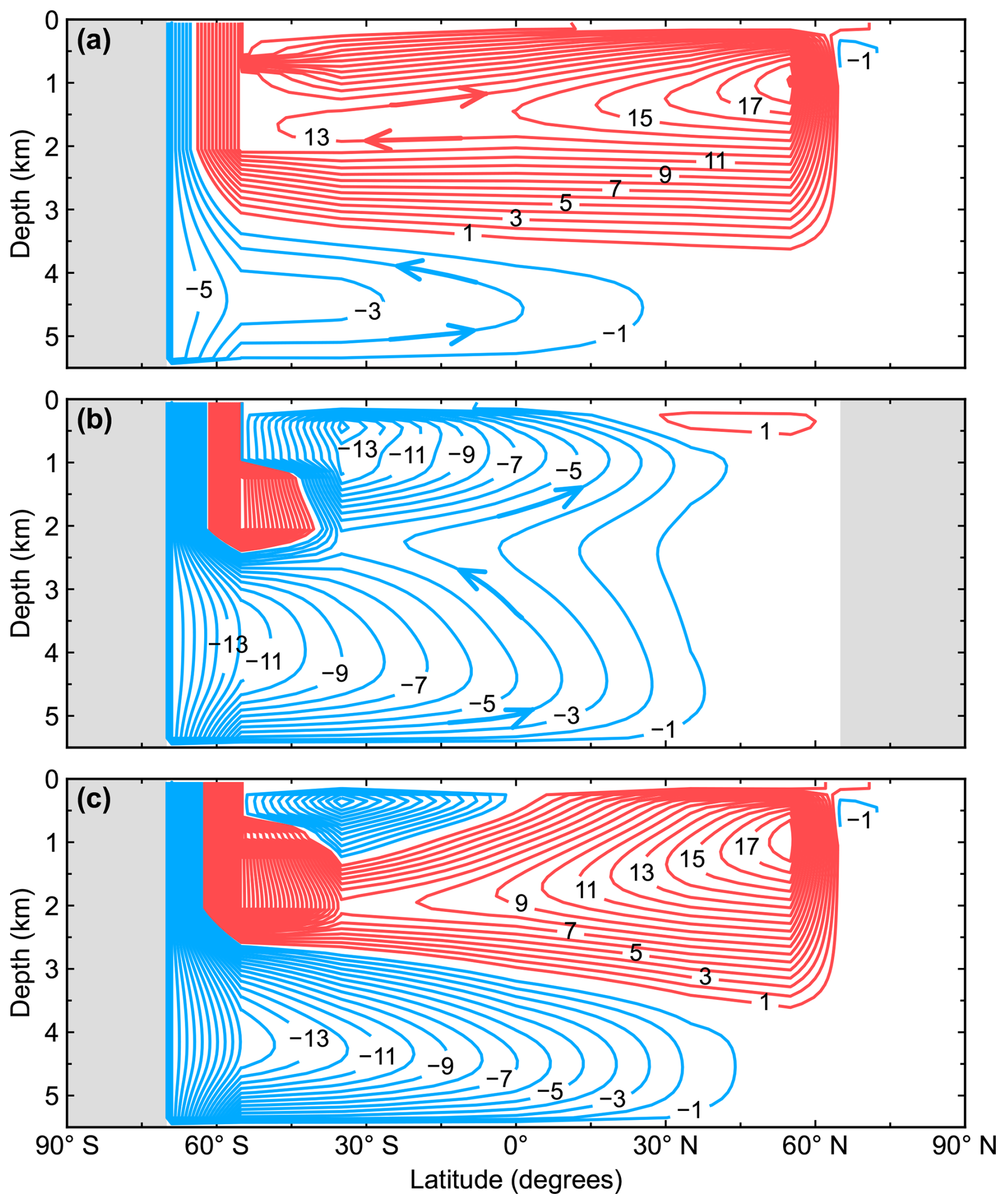
Figure 3 Pre-industrial, steady-state model representation of the meridional overturning circulation (Sv) for (a) the Atlantic Ocean, (b) the Pacific Ocean and (c) the global ocean. Red contours (positive values) represent clockwise circulation, and blue contours (negative values) represent counterclockwise circulation, as indicated schematically by arrows.

The Pacific Ocean overturning circulation is dominated by a counterclockwise cell carrying AABW which fills the whole deep ocean. The lower branch of the northward flow in this cell upwells in the North Pacific and returns southward in a near-surface flow. The upper branch of the northward flow in this cell upwells and returns southward to the Southern Ocean below 2000 m without crossing the Equator. There is also a second counterclockwise cell carrying Antarctic Intermediate Water (AAIW) north of the Equator above 2000 m depth. The upper southward branch of this cell joins the southward, near-surface flow of the deep counterclockwise cell described above. There is a weak clockwise cell confined above 500 m depth in the North Pacific related in part to the imposed model outflow to the Arctic Ocean through the Bering Strait.

The mediterranean Arctic Ocean presents an estuarine-type meridional circulation of 1 Sv intensity entering at 700 m depth and flowing out at 300 m depth. This counterclockwise circulation is maintained mainly by the zonally averaged geometry and freshwater inputs from precipitation and runoff. The Southern Ocean shelf produces 5.4 Sv of overflow water, which after entrainment increases its volume to ∼ 16 Sv upon outflow in the deep Southern Ocean. This agrees quite well with observed estimates (Orsi et al., 2002; Gordon, 2019). Such realistic entrainment and subsequent AABW formation, as achieved in the model with the prescribed present-day Antarctic continental slope (Amante and Eakins, 2009), underline the usefulness of our simplified gravity current approach to this problem.

Northward ocean heat transport is found throughout the Atlantic Ocean, peaking at 35° N with 0.83 PW and falling subsequently to 0.75 and 0.19 PW at 55 and 65° N, respectively. The high value at 55° N is related to the maximum ocean circulation intensity there. The South Atlantic carries 0.37 and 0.34 PW northward at 35 and 55° S, respectively. The North Pacific Ocean transports heat northward, with values of 0.41 and 0.29 PW at 35 and 55° N, respectively. The South Pacific Ocean transports heat southward, peaking at 35° S with 1.21 and 0.84 PW at 55° S. At the Equator, the Atlantic and the Pacific oceans transport heat in opposite directions with 0.65 PW northward and 0.37 PW southward, respectively. All modeled ocean transports agree well with data-based estimates (Trenberth and Caron, 2001), except at 55° N, where the modeled value is greater than observations.

3.1.5 Ocean tracer and biological-production results

Model ocean profiles of T, S and δ¹⁸O_w are plotted together with observational data in Fig. 4 (all observed data shown in Figs. 4–7 are from the Global Ocean Data Analysis Project version2.2022 (GLODAPv2; Lauvset et al., 2022), except for those of δ¹⁸O_w, where data are from the Global Seawater Oxygen-18 Database – v1.22 (Schmidt, 1999; Bigg and Rohling, 2000) have been used). In general, there is good model–data agreement, especially at mid-depths and in the deep and abyssal ocean. In the upper ocean, the model profiles are well within the observed mean range values. In particular for temperature, the model captures surface–deep-ocean transitions quite well in most of the model ocean sectors. Modeled temperatures in the Arctic Ocean below 1000 m are about 3.5 °C warmer than observations, likely reflecting the extensive ocean area covered by sea ice and/or the lack of local deepwater formation mechanisms like wintertime coastal polynyas in our simplified model. South of 35° S, model temperature falls at the warm end of the observed data.

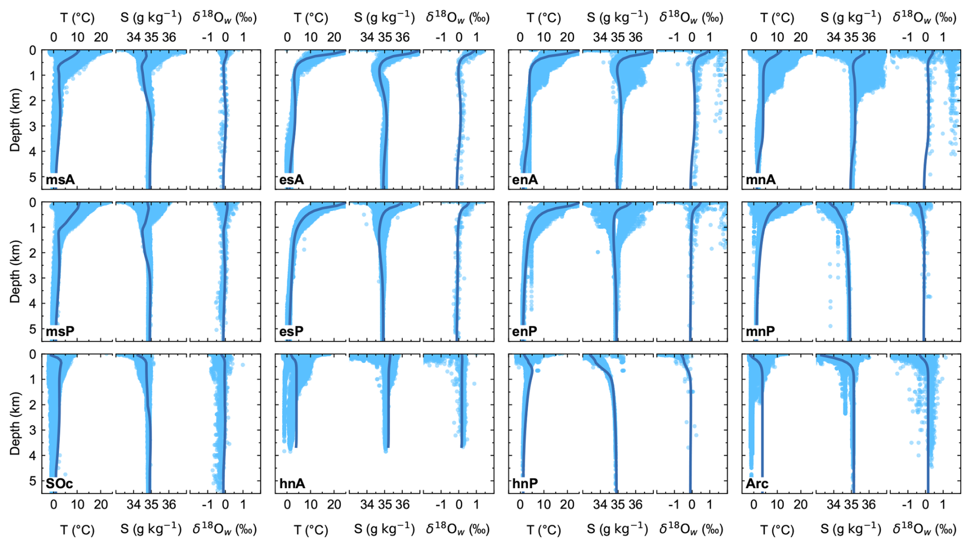
Figure 4 Pre-industrial, steady-state model ocean vertical profiles (dark-blue lines) of conservative temperature (T), absolute salinity (S) and water ¹⁸O isotopic excursion (δ¹⁸O_w) compared to observed data (light-blue dots) for each ocean model sector shown in Fig. 1a. T and S are compared with data from the GLODAPv2 database (Lauvset et al., 2022); δ¹⁸O_w values are compared with data from the Global Seawater Oxygen-18 Database – v1.22 (Schmidt, 1999; Bigg and Rohling, 2000, https://data.giss.nasa.gov/o18data/, last access: 23 November 2023).

Model salinity is quite well represented and captures prominent features of the global ocean, such as the salinity minimum at 650 and 1050 m depth for the msA and msP sectors representing the AAIW; the relative surface minimum in the mnP and hnP sectors associated with North Pacific Intermediate Water (NPIW; Sverdrup et al., 1942); and the vertical salinity structure in the Arctic Ocean with a surface salinity minimum, associated with freshwater inputs from runoff, sea ice melt and snowmelt and the strong halocline as found in observations (Aagaard et al., 1981). The lack of equatorial upwelling in our simplified model may explain the relatively warm and salty waters in the northern and southern tropical sectors. For δ¹⁸O_w, the model captures the vertical distribution as well as the meridional gradient in each model sector well, reflecting the global evaporation–precipitation distribution associated with isotopic fractionation of water.

Model ocean profiles of PO₄ and O₂ are plotted together with observational data in Fig. 5. The model achieves a good fit to the observed values in almost all ocean model sectors although the model results for O₂ are slightly lower than observed for the mid-depth Atlantic Ocean. Surface phosphate is strongly controlled by ocean new production. Low surface values are found in all ocean sectors, except at the Southern Ocean, where the highest surface values are found due to intense upwelling and to the low biological-production efficiency, as expected from the low value of L_f in our model. Furthermore, the model captures differences between the Pacific Ocean and Atlantic Ocean basins well. These differences are largely a consequence of the large-scale ocean circulation as described above. The oldest waters are found at the North Pacific Ocean (model sectors mnP and hnP; see Δ¹⁴C model profiles in Fig. 6), and consequently, the highest (lowest) values of phosphate (dissolved oxygen) in the ocean interior are found there. High dissolved O₂ values both at the surface and in the abyssal ocean are relatively well represented in the model in response to air–sea gas exchange and AABW ventilation. At the ocean interior, O₂ distributions respond mainly to organic matter remineralization and, for the msA and msP sectors for example, ventilation from AAIW. Misrepresentation of PO₄ and dissolved O₂ above 1000 m depth in the hnP sector is related to the way NPIW is treated in the model. The PO₄ (dissolved O₂) excess (deficit) in the Arctic model sector is related to the overestimation in ocean temperature there, which influences organic matter remineralization.

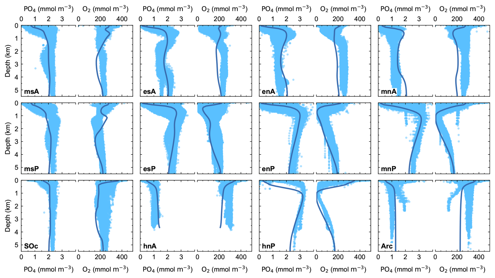
Figure 5 Pre-industrial, steady-state model ocean vertical profiles (dark-blue lines) of phosphate (PO₄) and dissolved oxygen (O₂) compared to observed data (light-blue dots) for each ocean model sector shown in Fig. 1a. Observed values are from the GLODAPv2 database (Lauvset et al., 2022).

The ocean carbon cycle model tracers DIC and ALK are plotted together with observed DIC and ALK in Fig. 6. The comparison with observational data shows excellent model–data agreement for both DIC and ALK. Both the vertical structure and the spatial differences among ocean model sectors are well captured by the model. Furthermore, both the depths of the DIC maximum and the slightly shallower depths of the PO₄ maximum (Fig. 5) in well-stratified ocean zones agree well with observations, indicating good e-folding length choices used for model remineralization rates. These distributions reflect the interplay between the cycling of organic matter and calcite as well as the air–sea exchange of CO₂.

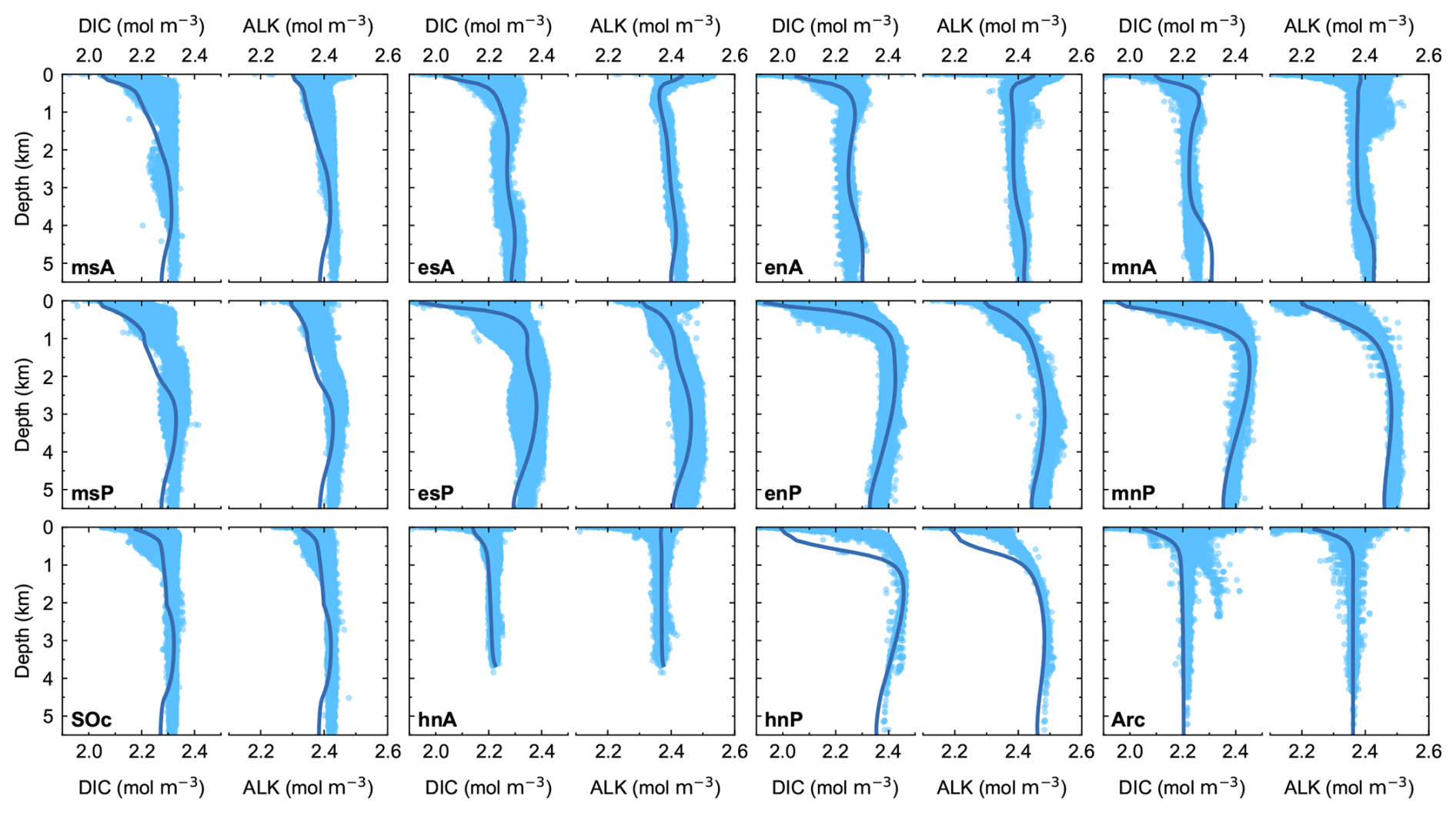
Figure 6 Pre-industrial, steady-state model ocean vertical profiles (dark-blue lines) of total dissolved inorganic carbon (DIC) and alkalinity (ALK) compared to observed data (light-blue dots) for each ocean model sector shown in Fig. 1a. Observed values are from the GLODAPv2 database (Lauvset et al., 2022).

Vertical distributions of carbonate ion (${\mathrm{CO}}_{\mathrm{3}}^{\mathrm{2}-}$), ${\mathrm{CO}}_{\mathrm{3}}^{\mathrm{2}-}$ saturation with calcite (${\mathrm{CO}}_{\mathrm{3},\mathrm{sat}}^{\mathrm{2}-}$) and water CO₂ are plotted in Fig. 7. The crossing point between ${\mathrm{CO}}_{\mathrm{3}}^{\mathrm{2}-}$ and ${\mathrm{CO}}_{\mathrm{3},\mathrm{sat}}^{\mathrm{2}-}$ is the calcite saturation depth (CSD), which is found to be at around 4000 m depth for the entire Atlantic Ocean and which reaches a minimum depth of around 700 m in the North Pacific sector, where the maximum water CO₂ concentration even exceeds that of ${\mathrm{CO}}_{\mathrm{3}}^{\mathrm{2}-}$. These results showing undersaturation throughout most of the deep North Pacific Ocean would imply low values of CaCO₃ in ocean sediments there. This is confirmed by the results for modeled and observed ocean sediments presented below.

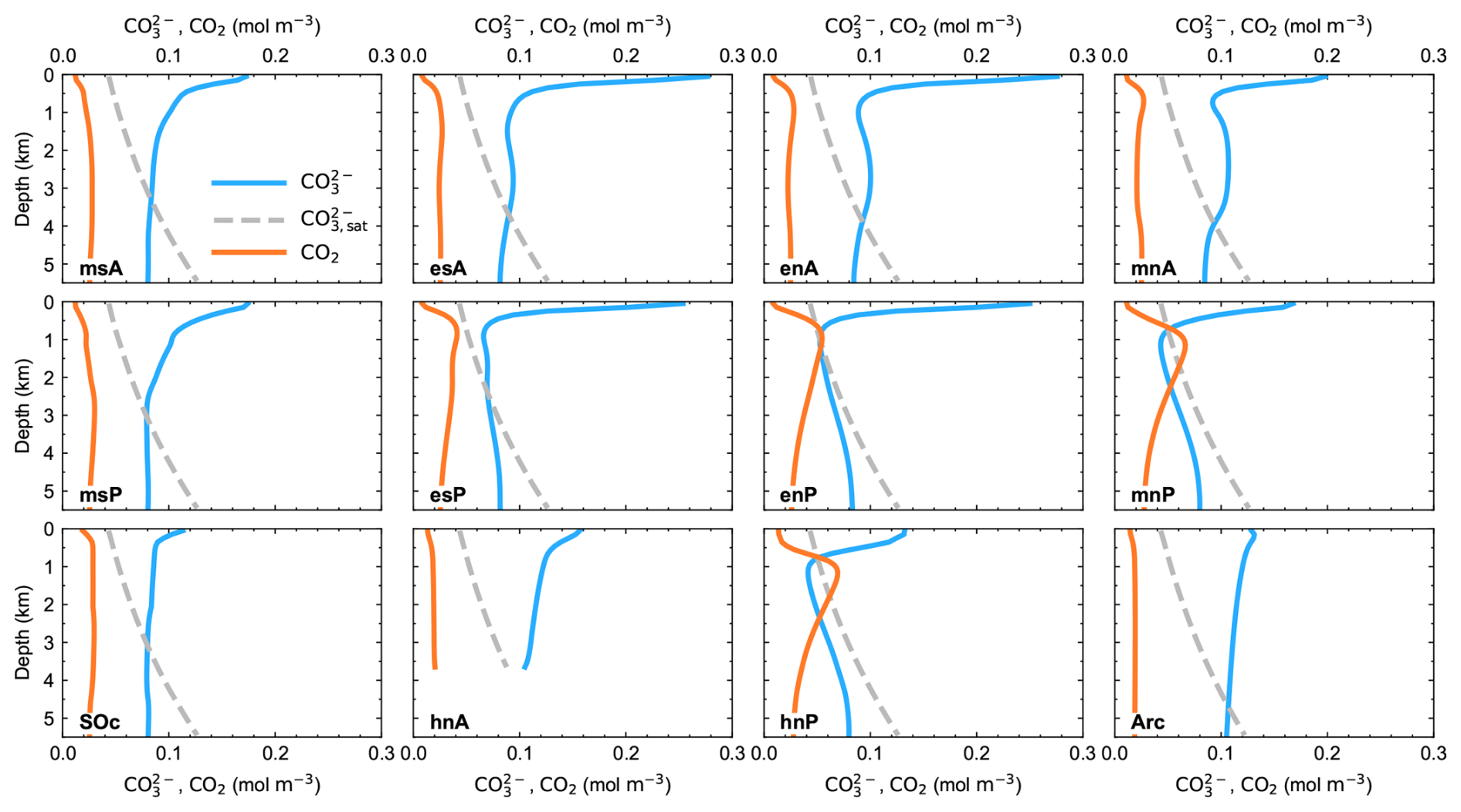
Figure 7 Pre-industrial, steady-state model ocean vertical profiles of carbonate ion (${\mathrm{CO}}_{\mathrm{3}}^{\mathrm{2}-}$), carbonate ion saturation with calcite (${\mathrm{CO}}_{\mathrm{3},\mathrm{sat}}^{\mathrm{2}-}$) and water CO₂ for each ocean model sector shown in Fig. 1a.

Ocean carbon isotopes (δ¹³C and Δ¹⁴C) are plotted together with observational data in Fig. 8. As with DIC and ALK, there is excellent model–data agreement in nearly all model ocean zones. As light carbon is preferentially taken up during photosynthesis, export of organic matter leaves the euphotic zone enriched in ¹³C (higher values of δ¹³C). Upon remineralization of this organic matter at depth, light carbon is released into the water column, leaving the water there depleted in ¹³C (lower values of δ¹³C). As shown by the agreement of model δ¹³C results with ocean as well as atmosphere data, the model deals well with this fractionation process as well as with the temperature-dependent fractionation associated with air–sea exchange of CO₂. As for PO₄ and O₂, meridional gradients and Pacific–Atlantic Ocean differences reflect ocean circulation, as seen clearly in the Δ¹⁴C profiles. The oldest waters are found in the North Pacific and exhibit the most negative values of δ¹³C and Δ¹⁴C in the ocean interior due to a longer time for receiving light carbon from organic matter remineralization and a longer time for radioactive decay to act, respectively. Modeled surface ocean δ¹³C values are well within the data-based estimates, with a global surface mean model result of 2.15 ‰. As before, the model–data disagreement of δ¹³C in the upper 1000 m depth in the hnP sector is related to NPIW formation in the model.

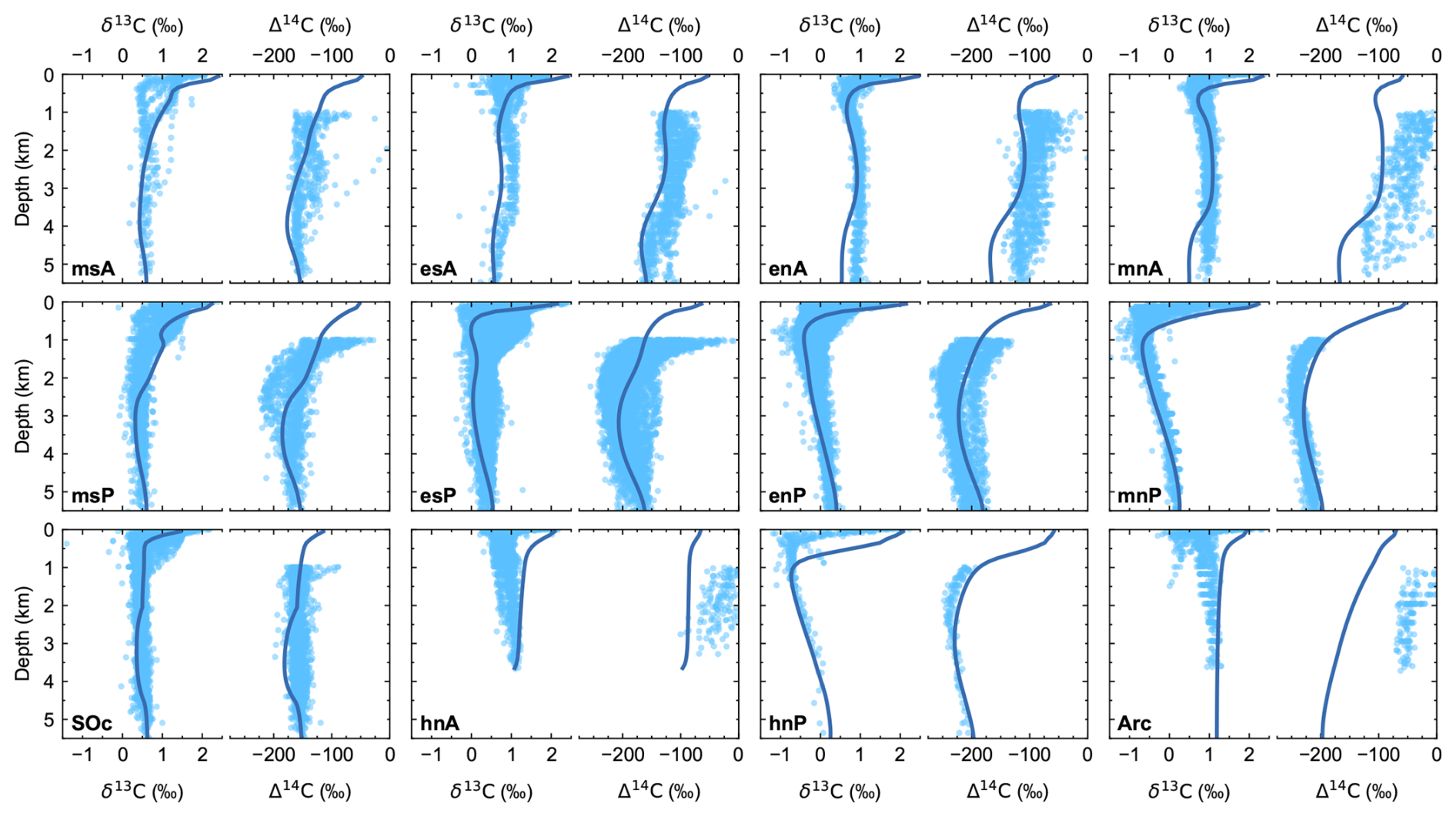
Figure 8 Pre-industrial, steady-state model ocean vertical profiles (dark-blue lines) of isotopic excursion of ¹³C (δ¹³C) and isotopic excursion of ¹⁴C (Δ¹⁴C) compared to observed data (light-blue dots) for each ocean model sector shown in Fig. 1a. Observed values are from the GLODAPv2 database (Lauvset et al., 2022). For Δ¹⁴C, only values below 1000 m depth have been plotted as shallower depths are strongly affected by the anthropogenic signal including atomic-bomb ¹⁴C inputs. Note that bomb ¹⁴C also affects deeper levels in the North Atlantic and Arctic sectors (mnA, hnA and Arc).

With all the above and despite minor model–data disagreement, the model reproduces the main global features of both physical and biogeochemical tracers quite well. Better ocean modeled distributions of S, δ¹⁸O_w, DIC, ALK, δ¹³C and Δ¹⁴C are key improvements that have been made in comparison to the much simpler DCESS I model, where distributions of those tracers had shortcomings, in particular for S, δ¹⁸O_w and δ¹³C (Shaffer et al., 2008).

Model global ocean new (exported) production (NP) is 5.84 Gt C yr⁻¹, slightly higher than the 5.4 Gt C yr⁻¹ of the DCESS I model (Shaffer et al., 2008). This new estimate is at the lower end of the estimates from Dunne et al. (2007) (9.6 ± 3.6 Gt C yr⁻¹) but almost matches a modern and possibly more robust estimate of Siegel et al. (2014) of 5.90 Gt C yr⁻¹. The tropical ocean model zones (35° S–35° N) are by far the most productive model regions, accounting for more than 66 % of global exported production partitioned into 53 % and 13 % for the Pacific and Atlantic oceans, respectively. The Arctic Ocean and high-latitude northern zone of the Pacific Ocean have the lowest values of exported NP, with 0.2 % and 1.1 % of the total, respectively. The Southern Ocean also has a rather low value, with 5 % of total export production. Northern and southern mid-latitude model sectors (35–55° N/S) show around 22 % of total NP, with 5 % and 7 % for the mnP and mnA sectors, respectively, and 8 % and 2 % for the msP and msA sectors, respectively. This meridional distribution is also observed in the publications cited above. We believe that the lack of equatorial upwelling of nutrient-rich waters in the model probably contributed to the relatively low value of ocean NP in our model.

Global biogenic calcite production in the model is 1.25 Gt C yr⁻¹, and more than 65 % is produced in tropical model zones of the Pacific Ocean. Tropical zones of the Atlantic Ocean account for only 16 % of global calcium carbonate production. Extratropical ocean model zones from the Northern Hemisphere and Southern Hemisphere, combining the Pacific and Atlantic sectors, represent only 15 % of total biogenic calcite production. Table 4 shows values for organic matter and calcite production for each ocean model sector.

Table 4 Pre-industrial organic matter and biogenic calcite ocean production estimates. All values are given in Gt C yr⁻¹.

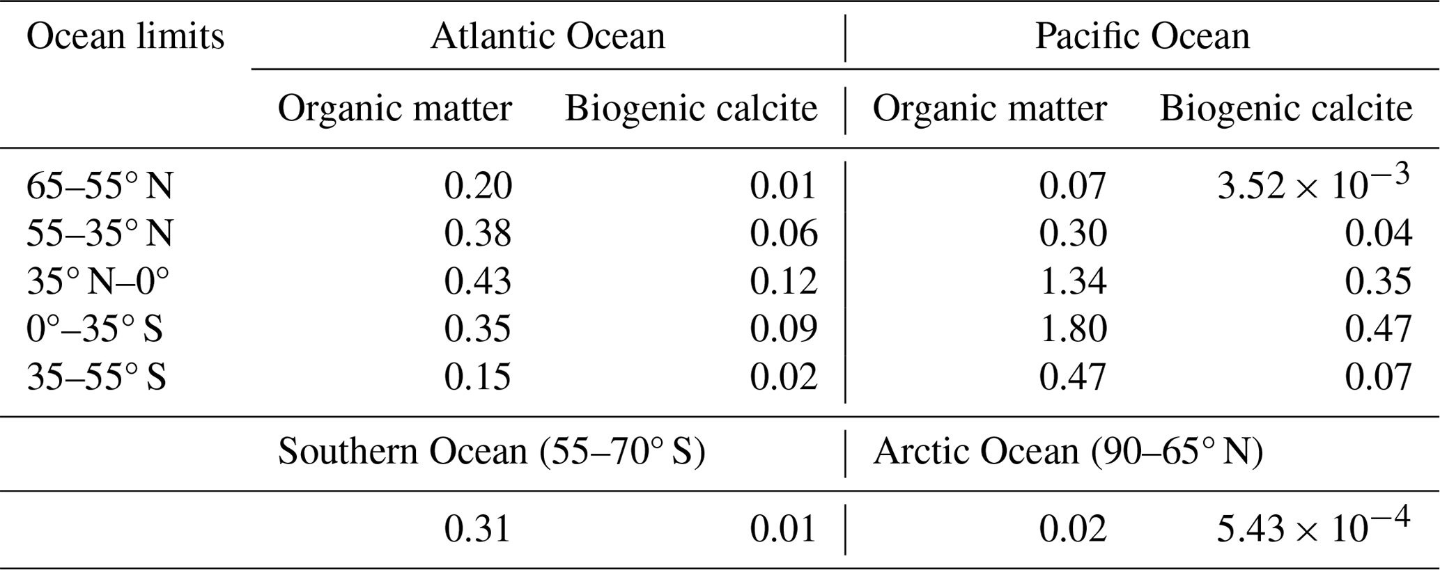
Our estimates are well into the observed range of 0.5–1.6 Gt C yr⁻¹ of Berelson et al. (2007) but slightly higher than more recent estimates of 0.91 ± 0.14 Gt C yr⁻¹ (Sulpis et al., 2021). Overall, our model result of new (exported) production is well into the range of CMIP6 models (Planchat et al., 2023), but our biogenic calcite production is at the upper end of those model estimates. However, we note that CMIP6 ensemble results tend to globally underestimate the exported inorganic carbon compared to observational estimates (Planchat et al., 2023).

The calcite carbon-to-organic carbon flux ratio is similar for the Pacific/Atlantic oceans, with ratios of $\mathrm{0.6}/\mathrm{0.5}$, $\mathrm{0.9}/\mathrm{0.7}$ and $\mathrm{1.2}/\mathrm{1.1}$ in the tropical model sectors at 1000, 2000 and 3000 m depth, respectively, and ratios of 0.2, 0.3 and 0.5 for northern-latitude sectors of those basins at these depths. These ratios are somewhat lower than those estimated from sediment trap data (Berelson et al., 2007). The longer e-folding scale ξ_Cal than ξ_C and the temperature effect on organic matter remineralization and on the CaCO₃ rain ratio (see Sect. 2.4) help explain these results.

3.1.6 Sediment results

In the model pre-industrial steady state, 0.11 Gt C yr⁻¹ of organic carbon is buried in ocean sediments. This represents 12 % of total organic carbon falling on the sediment surface; the remaining 88 % is remineralized to DIC, which returns to the water column. This modeled value is well within the range of data-based estimations (Berner, 1982; Hedges and Keil, 1995; Cartapanis et al., 2018). However, the higher ends of some of these estimates may include contributions from estuaries and delta environments that our model does not consider. Other modeled results are in the range of 0.02–0.09 Gt C yr⁻¹ (Berner, 1991; Munhoven, 2007; Willeit et al., 2023). More than 90 % of our modeled burial takes place at water depths shallower than 1000 m such that 0.011 Gt C yr⁻¹ is buried below this depth, in agreement with deep-sea burial estimates (Hayes et al., 2021). The highest modeled burial rates for organic carbon per ocean sector are found in the tropical Pacific Ocean and the North Atlantic Ocean (35–65° N) sectors with over 40 % and 27 %, respectively, of the total organic carbon burial. The global inventory of bioturbated-layer (BL) organic carbon is 122 Gt C, somewhat higher than that found in the pre-industrial DCESS I model simulation (92 Gt C).

For calcite, the global annual mean burial rate is 0.21 Gt C yr⁻¹, and more than 57 % takes place in the tropical Pacific sectors and 23 % is buried at the combined northern tropical and mid-latitude Atlantic Ocean sectors. Our global result compares well with data-based estimations and model results in the range of 0.13–0.45 Gt C yr⁻¹ (Milliman and Droxler, 1995; Cartapanis et al., 2018; Hayes et al., 2021; Willeit et al., 2023). Of the total annual mean burial rate of CaCO₃ in the Pacific and Atlantic oceans (0.14 and 0.07 Gt C yr⁻¹, respectively), 49 % and 45 % of calcite, respectively, is buried at depths greater than 1000 m in these basins. Other estimates also show such a nearly half-and-half shelf-slope vs. deep-ocean division (Milliman, 1993). The modeled global ocean mean calcite dry-weight fraction (CaCO₃)_dwf is 0.349, whereas the Pacific and Atlantic oceans present mean values of (CaCO₃)_dwf of 0.353 and 0.440, respectively, where the highest values are found in the tropical South Pacific and North Atlantic sectors, with values of 0.459 and 0.553, respectively. The model global inventory of bioturbated-layer calcite carbon is 767 Gt C, somewhat lower than the DCESS I pre-industrial estimate (1010 Gt C) but in good agreement with the 800 Gt C data-based estimate from Archer (1996). Of this, 503 Gt C is found in the Pacific Ocean BL and 249 Gt C in the Atlantic Ocean one, equivalent to 66 % and 32 % of the total, respectively. The results above highlight how the model captures ocean carbon cycle differences between the Pacific and Atlantic oceans.

Figure 9 shows the dry-weight fractions of organic matter (OM)_dwf and calcite (CaCO₃)_dwf as well as the sediment velocity out of the bottom of the BL (w_sed) for each ocean model sector. In general, relatively high (OM)_dwf, relatively low (CaCO₃)_dwf and rapid sedimentation rates are found at shallow depths. This can be explained mainly by the high prescribed flux of non-calcite minerals at such depths that (1) fill the BL mainly with such minerals and (2) rapidly flush the BL, thereby promoting high (OM)_dwf burial since relatively little organic matter is remineralized in the BL on such short timescales. At intermediate depths above the model's CSD, (CaCO₃)_dwf is higher, (OM)_dwf is lower and sedimentation rates are more moderate. This results not only from enhanced CaCO₃ accumulation in sediments bounded by ocean layers supersaturated with carbonate ion (see Fig. 7), but also from much lower non-calcite mineral and organic matter rain rates, leading to slower BL flushing that allows more complete organic matter remineralization. At those intermediate depths, the modeled effect of dissolved oxygen on organic matter remineralization can be seen in the North Pacific model sectors, where this remineralization is slowed down considerably as ocean layers there become nearly suboxic/anoxic. This also leads to a local increase in sediment rates. In the deep ocean below the model's CSD, rapid decreases in CaCO₃ content, very low organic matter contents and slower sedimentation rates are the result of calcite dissolution combined with low constant non-calcite rain rates and still lower organic matter rain rates. The Arctic Ocean model sediment is almost completely composed of non-calcite mineral because the sediment flux of biogenic material falling on the sediment surface is very small due to the extremely limited surface new production. In the Southern Ocean, model sediment is also composed mainly of non-calcite minerals but contains larger fractions of (OM)_dwf and (CaCO₃)_dwf than in the Arctic Ocean. The water depth of the calcite compensation depth (CCD), defined operationally where (CaCO₃)_dwf equals 0.1, is found at around 4800 m for both the tropical Pacific and the tropical Atlantic Ocean sectors. In contrast, there are major differences between the North Atlantic and North Pacific sectors, with CCD depths of around 4400 and 2100 m depth, respectively.

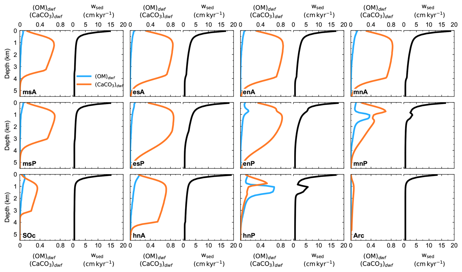
Figure 9 Pre-industrial, steady-state model sediment vertical profiles of dry-weight fractions of organic matter, (OM)_dwf, and calcite, (CaCO₃)_dwf, as well as sedimentation velocity (w_sed), all at the base of the bioturbated layer of each ocean model sector shown in Fig. 1a.

3.1.7 Lithosphere results

Table 5 lists model weathering and burial rates for the pre-industrial steady state. From weathering–burial steady-state balances outlined in Sect. 2.7 and global mean values of ¹³C isotope excursions for organic carbon (δ¹³OrgC = −22.06 ‰) and carbonate (δ¹³Carb = 2.22 ‰) obtained from the fifth calibration step, modeled outgassing from volcanoes is found to be 0.140 Gt C yr⁻¹, in good agreement with modern-day data-based estimates (IPCC, 2021). Results for carbonate and silicate weathering rates are similar to those found with the DCESS I model, 0.109 and 0.092 Gt C yr⁻¹, respectively (Shaffer et al., 2008). Our carbonate weathering rate is well into the range of other observational and model estimates, 0.088–0.241 Gt C yr⁻¹, but our silicate weathering rates are somewhat lower than other corresponding estimates, 0.122–0.236 Gt C yr⁻¹ (Gaillardet et al., 1999; Ludwig et al., 1999; Munhoven, 2002; Hartmann et al., 2009; Lenton et al., 2018; Willeit et al., 2023). Phosphorus weathering rates are higher than those found in the DCESS I model, 1.663 × 10³ mol P s⁻¹, but are in better agreement with observational estimates, 2.019 × 10³–3.071 × 10³ mol P s⁻¹ (Filippelli, 2002; Paytan and McLaughlin, 2007). Organic carbon weathering rates agree well with recent estimations of 0.068 Gt C yr⁻¹ (Zondervan et al., 2023). Based on these results, although simple, our continental weathering–climate relationship gives reasonable results when compared against models with more complicated relationships.

Table 5 Weathering, lithosphere outgassing and burial estimates for pre-industrial, steady-state balances.

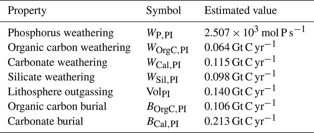
The modeled river input of total inorganic carbon is 0.43 Gt C yr⁻¹, a value close to that found in the DCESS I model (0.40 Gt C yr⁻¹) and close to the 0.41 Gt C yr⁻¹ from data-based estimates (Li et al., 2017). More than 51 % of this river input flux is delivered to the Atlantic Ocean, while 40 % drains into the Pacific Ocean and the rest into the Arctic Ocean. The Southern Ocean does not receive inorganic carbon from rivers. With the results above, modeled steady-state, pre-industrial global ocean outgassing of CO₂ is 0.11 Gt C yr⁻¹, which is balanced by net uptake of atmospheric CO₂ that is expressed as $\mathrm{2}{W}_{\mathrm{Sil},\mathrm{PI}}+W_{\mathrm{Cal},\mathrm{PI}}-({\mathrm{Vol}}_{\mathrm{PI}}+W_{\mathrm{OrgC},\mathrm{PI}}$).

3.2 Testing the model

We carry out two simple experiments to test model performance. In the first experiment (Exp 1), we force the model with an imposed, time-dependent function of northward Ekman transport out of the Southern Ocean at 55° S. We considered two cases for this experiment, doubling (Exp 1a) and halving (Exp 1b) this transport value on a timescale of 1500 years. With this, we try to emulate the role of Southern Ocean westerly winds in large-scale ocean circulation as it has been hypothesized that intensity and position shifts of these winds may drive global-scale climate changes on glacial–interglacial timescales (Gray et al., 2023; Lee et al., 2011; Toggweiler et al., 2006). In the second experiment (Exp 2), we force the model with an imposed, time-dependent function of freshwater input to the Southern Ocean shelf to emulate a melting pulse of the Antarctic ice sheet. We “melt” the equivalent of 2.5 × 10¹⁵ m⁻³ of freshwater (equivalent to 5 m sea level rise) over two different timescales: a fast pulse to get a sea level rise of 1 m (Exp 2a) and a slow pulse to get a 0.1 m rise (Exp 2b) after 250 years of model simulation. This is consistent with modeled assessments about Antarctic ice sheet retreats in the present climate context (Ruckert et al., 2017; DeConto and Pollard, 2016). In both experiments, we focus on changes in large-scale ocean circulation and their impact on ocean tracer distributions as well as on the global climate.

3.2.1 Southern Ocean Ekman transport forcing

The forcing and model results are presented in Fig. 10. With the increase in northward Ekman transport (Exp 1a) across 55° S, there is more upwelling in the Southern Ocean sector (Fig. 10b). However, this Southern Hemisphere forcing does not significantly impact AMOC intensity in the North Atlantic Ocean, as shown by the streamline evolution at 55° N at 1000 m depth (Fig. 10e). Rather, this forcing leads to the appearance of a clockwise recirculation cell between 55 and 40° S confined between 1000 and 2000 m depth for both the Atlantic and the Pacific oceans, as indicated by the vertical flux (defined as positive upward) in the msA and msP sectors at 1500 m depth shown in Fig. 10c–d. In Exp 1b, a decrease in northward Ekman transport across 55° S causes a decrease in the Southern Ocean upwelling (Fig. 10b). In this experiment there is an increase in the upward flux above 2000 m depth in msA and a decrease in the downward flux below 1000 m depth in msP, fluxes that subsequently join the upper-ocean northward flow and the deep southward flow in the Atlantic and Pacific oceans, respectively. The insensitivity of North Atlantic AMOC intensity as well as of intermediate-depth Southern Hemisphere recirculation to increased westerly forcing has also been reported in other modeled experiments (Jochum and Eden, 2015; Rahmstorf and England, 1997).

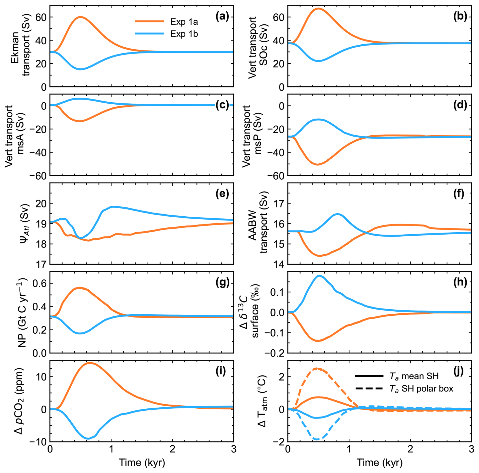
Figure 10 Results for 3000-year simulations for two different choices of northward Ekman transport across 55° S. (a) Applied Ekman transport evolutions; (b–d) vertical transport (Vert transport, defined as positive upward) at 1500 m depth for the Southern Ocean, msA and msP sectors, respectively; (e) northward transport across 55° N above 1000 m depth in the Atlantic Ocean; (f) AABW transport reaching the abyssal Southern Ocean; (g–h) Southern Ocean new-production evolution and Southern Ocean surface δ¹³C change; and (i–j) changes in atmospheric CO₂ and atmospheric temperature (solid lines denote Southern Hemisphere mean T_a, and dashed lines denote T_a for the atmospheric southern polar zone, 55–90° S).

These ocean interior circulation changes lead to a denser (lighter) water being upwelled in the Southern Ocean for Exp 1a and Exp 1b, respectively, leading to less (more) entrainment and consequently decreasing (increasing) amounts of AABW reaching the abyssal ocean for these experiments (Fig. 10f). More (less) upwelling together with this Southern Hemisphere recirculation enhances (reduces) ocean new production in the Southern Ocean, as more (fewer) nutrients are carried to the surface there (Fig. 10g). These changes in Southern Ocean NP are not reflected in surface ocean δ¹³C values (Fig. 10h, as well as in msA and msP) in this zone of low model new-production efficiency. Rather, the decrease (increase) in δ¹³C values in Exp 1a (Exp 1b) is associated with a lighter (heavier) signal of ¹³C from more (less) upwelling of deeper water originating from northern latitudes of Atlantic and Pacific model zones. Air–sea exchange of CO₂ with the Southern Ocean reflects changes in the upwelling rates there as more or less carbon-rich deeper water is carried to surface layers there. More (less) outgassing there leads to an increase (decrease) in atmospheric CO₂ concentration (Fig. 10i) and a resulting rise (fall) in atmospheric temperature (Fig. 10j). Such a Southern Hemisphere westerly wind intensity–atmospheric CO₂ relationship has also been reported in another modeled experiment (d'Orgeville et al., 2010). Changes in atmospheric CO₂ content are nearly uniform in all atmospheric boxes due to the rapid turnover time of the atmosphere. The temperature change in the southern polar atmospheric box is around 2.5 and −1.8 °C for Exp 1a and Exp 1b, respectively. However, this warming (cooling) signal decreases rapidly farther northward such that mean Southern Hemisphere atmospheric temperature changes are around 0.7 and −0.5 °C for Exp 1a and 1b, respectively. Finally, our Exp 1a results are in line with the importance of Southern Hemisphere westerly winds for deglacial atmospheric CO₂ rise as found in models and proxy-data reconstructions (Mayr et al., 2013; Menviel et al., 2018).

3.2.2 Antarctic ice sheet melt freshwater forcing

Forcing and model results for this experiment are shown in Fig. 11. The rapid freshwater pulse to the Southern Ocean shelf (Exp 2a) produces a greater and more abrupt decrease in AABW fluxes flowing down off the shelf break (F_sl,0), as well as in the abyssal ocean, F_sl (Fig. 11b). For Exp 2a, F_sl,0 and F_sl reach minimum values of 3.5 and 11 Sv, respectively, i.e., around 30 % less than the pre-industrial values. In Exp 2b, modest declines of 0.7 and 2 Sv are obtained for F_sl,0 and F_sl, representing a decrease of only 13 % compared to modern-day values (Gordon, 2019). Such an effect on AABW production rates due to Antarctic meltwater on the Southern Ocean shelf has been observed in similar Antarctic-meltwater experiments using more complex models (Fogwill et al., 2015; Silvano et al., 2018; Li et al., 2023). Consequently, the abyssal counterclockwise circulation decreases its intensity by more than 11 and 2 Sv for fast and slow freshwater pulses, respectively, as shown by the northward streamline evolution at 4500 m depth crossing 55° S (Fig. 11c). Such behavior has been reported for numerous model experiments including a multi-model ensemble of CMIP6 model experiments (Park and Latif, 2019; Mackie et al., 2020; Chen et al., 2023). This corresponds to a 75 % decrease compared to only a 14 % decrease for the fast and slow freshwater pulses, respectively, underlining the sensitivity of model AABW circulation to not only the size but also the speed of the Antarctic ice sheet meltwater pulse. Such lower AABW ventilation rates lead to the decline in dissolved O₂ content of the abyssal northern sectors of the Pacific and Atlantic oceans (Fig. 11d–e). This suggests aging of the abyssal ocean, also reported in Li et al. (2023). A greater AMOC penetration depth, as a consequence of weakened AABW abyssal circulation, may inhibit a further decrease in the abyssal O₂ content of the North Atlantic Ocean as more atmospheric oxygen is carried to those depths.

Opposite behaviors are observed in the abyssal ocean Δ¹⁴C content for the northernmost model sectors of the North Atlantic and North Pacific oceans (hnA and hnP, respectively). The increase in the hnA sector (Fig. 11f) is caused by deeper AMOC penetration depth as the AABW cell gets weaker, leading to increased transport of near-surface ¹⁴C to the abyssal ocean. In the hnP sector, the decrease in ¹⁴C content stems from longer residence times due to the reduced AABW ventilation there, leading to more radioactive decay. The ¹⁸O signature in the abyssal ocean is quite sensitive to the freshwater forcing to the Southern Ocean shelf as meltwater from the Antarctica ice sheet comes with an isotopic signal of −40 ‰ in the model. This is shown in Fig. 11h–i, where similar changes are observed in the sectors directly north of the Southern Ocean (msA and msP) at 4500 m depth, with changes of around −0.17 ‰ and −0.09 ‰ for fast and slow forcing experiments, respectively. This demonstrates the model's ability to capture the δ¹⁸O_w signal from Antarctic ice sheet melting, shown to be a better indicator of such melting than ocean salinity changes (Kim and Timmermann, 2024). Despite all these ocean interior changes, Exp 2a and Exp 2b forcings lead only to small changes in atmospheric CO₂ of around 1 ppm or less in both experiments. As a consequence, there is nearly no change in the global atmospheric temperature although small sea-ice-dynamics-driven oscillations of a 20-year period are found in the southern polar atmospheric temperature (not shown). We stress that this simplified experiment was carried out mainly to test the model performance under isolated freshwater forcing. A comprehensive study of the global climate system response to Antarctic ice sheet melting would also require consideration of the climatic effects leading to the melting in the first place, i.e., a coupling of the climate system and the ice sheet.

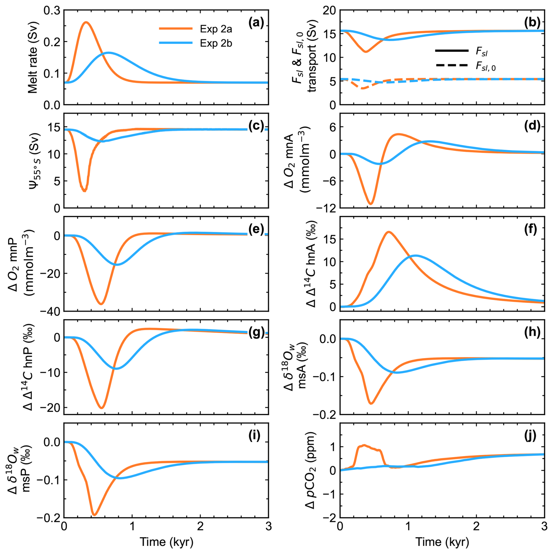
Figure 11 Results for 3000-year simulations for two different choices of Antarctic ice sheet melt rate. (a) Applied melt rates evolutions, (b) AABW transport flowing off the Southern Ocean shelf (F_sl,0) and reaching abyssal depths (F_sl), (c) total northward transport (combined Atlantic and Pacific) crossing 55° S below 4500 m depth, (d–e) changes in dissolved O₂ content in the ocean at 4500 m depth for northern sectors of the Atlantic and the Pacific Ocean, respectively (mnA and mnP), (f–g) ocean Δ¹⁴C change at 4500 m depth for the northernmost sectors of the Atlantic and the Pacific Ocean, respectively (55–65° N, hnA and hnP), (h–i) δ¹⁸O_w change at 4500 m depth for ocean sectors directly north of the Southern Ocean (msA and msP) and (j) global mean atmospheric pCO₂ change.

4 Discussion and conclusions

We have described and tested a new Earth system model of intermediate complexity, DCESS II, which has been calibrated to the pre-industrial Earth system. For this relatively simple model, efforts were made to limit the number of model free parameters and to constrain their values as much as possible using observations. At the end of this process, despite model limitations, we generally find excellent agreement with available modern observations. When compared with results from the DCESS I model, a number of improvements in our new model stand out, as described below.

Some key features of the physical part of the model, like the horizontal resolution, a simplified dynamical scheme for large-scale ocean circulation, stratification-dependent vertical diffusion, a gravity current approach to the formation of Antarctic Bottom Water and a dynamical formulation for sea ice, have helped us to achieve good agreement with observed data like atmospheric heat and water vapor transport and ocean temperature and salinity distributions (Lauvset et al., 2022) with a space and time resolution not possible using the original DCESS I model. These improvements, together with updates in ocean biogeochemistry such as a light dependence on the surface new (exported) production of organic matter, dependence on the calcite saturation state for the biogenic carbonate production and local temperature dependence on organic matter remineralization, result in accurate model representations of ocean biogeochemical tracers, highlighted by excellent model–data agreement with regard to marine carbon cycle species, well beyond that achieved with the DCESS I model, in particular with respect to ¹³C (Shaffer et al., 2008). Furthermore, the incorporation of a new land biosphere module with three different vegetation types and a light–atmospheric CO₂ dependence on net primary production on land, as well as ocean sediment and lithosphere modules applied to multiple ocean and land sectors, makes results of the new model much more amenable to comparison with data than is the case for the DCESS I model. All the above improvements help make the DCESS II model an excellent yet economical tool for studying and gaining short- as well as long-term understanding of the global carbon cycle.

Two experiments were conducted in order to explore and test model performance. In the first experiment (Exp 1) we forced the model in a way that emulates the role of the Southern Hemisphere westerly winds in large-scale ocean circulation. In the second experiment (Exp 2) we introduced (at two different rates) a freshwater melt volume equivalent to a global sea level rise of 5 m onto the shelf surrounding Antarctica. In both experiments, model results show important physical and biogeochemical changes in the ocean driving perturbations in the global carbon cycle. This is reflected in responses of atmospheric CO₂ as well as of abyssal ocean Δ¹⁴C and dissolved O₂ content. These experiments serve to demonstrate how the model captures the global role that Southern Hemisphere westerly winds and Antarctic Bottom Water play in the Earth system. Our Exp 1 supports the role of the Southern Hemisphere westerly winds in modulating past glacial–interglacial atmospheric carbon dioxide variations, while our Exp 2 points toward the impact that future Antarctic ice sheet melting would have on the formation of Antarctic Bottom Water and on the deep global ocean in general.

The development and calibration of the DCESS II model as described here have also set the stage for future work. For example, coupling of the model to an Antarctic ice sheet (AIS) model will provide a more realistic Earth system simulation when compared to our idealized experiment 2 described above. For this work an extended and improved version of the simple, well-tested DAIS model (Shaffer, 2014) will be used. In another example, planned incorporation of methane, nitrogen and sulfur cycles into the next DCESS II update will significantly improve its ability to deal realistically with deep-time global warming events associated with massive carbon inputs to the Earth system. Under such conditions, suboxic/anoxic ocean conditions may arise, leading, for example, to denitrification and sulfate reduction that must be addressed in such an update. Groundwork for this step has already been done in as much as these global biogeochemical cycles and suboxic/anoxic processes have been incorporated into the DCESS I model (Shaffer et al., 2017). In addition, other potential model applications include the study of different global climatic events like Dansgaard–Oeschger oscillations or longer climatic events like the Eocene–Oligocene transition or even the assessment of deep-time mass extinction events by taking advantage of the relative simplicity of the model for setting proper boundary conditions like orbital forcing and continental distribution. In this regard, when such deep-time model applications with quite different boundary conditions from today are to be made, careful consideration should be made in choosing the few (only two) regional tunings of the model.

In conclusion, we have presented, validated and tested a simple and fast new Earth system model of intermediate complexity intended to be a flexible, comprehensive and economical Earth system modeling platform. Despite its limitations like relatively low horizontal resolution and multiple parameterizations, the model represents most Earth system components quite well, especially the global-scale carbon cycle. Due to its simplicity, it could be easily modified in terms of boundary conditions to address specific past epochs. Thus, we find DCESS II to be a useful tool for studies of past, present and future global change on timescales of years to millions of years while not needing substantial computational resources.