Historical trends and controlling factors of isoprene emissions in CMIP6 Earth system models

Terrestrial isoprene, a biogenic volatile organic compound emitted by many plants, indirectly influences Earth's radiative balance through its interactions with atmospheric oxidants, affecting ozone formation, methane lifetime, and secondary aerosol production. Elucidating its historical changes is therefore important for predicting climate change and air quality. Isoprene emissions can respond to climate (e.g. temperature, shortwave radiation, precipitation), land use and land cover change (LULCC), and atmospheric CO₂ concentrations. However, historical trends of isoprene emissions and the relative influences of the respective drivers of those trends remain highly uncertain. This study addresses uncertainty in historical isoprene emission trends and their influential factors, particularly the roles of climate, LULCC, and atmospheric CO₂ (via fertilization and inhibition effects). The findings are expected to reconcile discrepancies among different modelling approaches and to improve predictions of isoprene emissions and their climate change effects.

To investigate isoprene emission trends, controlling factors, and discrepancies among models, we analysed long-term (1850–2014) global isoprene emissions from online simulations of CMIP6 Earth system models and offline simulations using the Vegetation Integrative SImulator for Trace gases (VISIT) dynamic vegetation model driven by climate reanalysis data.

Mean annual global present-day isoprene emissions agree well among models (434–510 TgC yr⁻¹) with a 5 % inter-model spread (24 TgC yr⁻¹), but regional emissions differ greatly (9 %–212 % spread). All models show an increasing trend in global isoprene emissions in recent decades (1980–2014), but their magnitudes vary (+1.27 ± 0.49 TgC yr⁻², 0.28 ± 0.11 % yr⁻¹). Long-term trends of 1850–2014 show high uncertainty among models (−0.92 to +0.31 TgC yr⁻²).

Results of emulated sensitivity experiments indicate meteorological variations as the main factor of year-to-year fluctuations, but the main drivers of long-term isoprene emission trends differ among models. Models without CO₂ effects implicate climate change as the driver, but other models with CO₂ effects (fertilization only/fertilization and inhibition) indicate CO₂ and LULCC as the primary drivers. The discrepancies arise from how models account for CO₂ and LULCC alongside climate effects on isoprene emissions. Aside from LULCC-induced reductions, differences in CO₂ inhibition representation (strength and presence or absence of thresholds) were able to mitigate or reverse increasing trends because of rising temperatures or in combination with CO₂ fertilization. Net CO₂ effects on global isoprene emissions show the highest inter-model variation (σ=0.43 TgC yr⁻²), followed by LULCC effects (σ=0.17 TgC yr⁻²), with climate change effects exhibiting more or less variation (σ=0.06 TgC yr⁻²).

The critical drivers of isoprene emission trends depend on a model's emission scheme complexity. This dependence emphasizes the need for models with accurate representation of CO₂ and LULCC effects alongside climate change influences for robust long-term predictions. Important uncertainties remain in understanding the interplay between CO₂, LULCC, and climate effects on isoprene emissions, mainly for CO₂. More long-term observations of isoprene emissions across various biomes are necessary, along with improved models with varied CO₂ responses. Moreover, instead of reliance on the current models, additional emission schemes can better capture isoprene emissions complexities and their effects on climate.

1 Introduction

Isoprene (2-methyl-1,3-butadiene, C₅H₈), a biogenic volatile organic compound (BVOC) emitted by terrestrial vegetation, strongly shapes our planet's atmospheric chemistry and climate (Fiore et al., 2012). This molecule, accounting for roughly half of global BVOC emissions (Guenther et al., 2012), interacts with atmospheric oxidants, influencing processes such as ozone formation (Arneth et al., 2010; Squire et al., 2014; Wiedinmyer et al., 2006), methane lifetime (Kaplan et al., 2006; Achakulwisut et al., 2015; Hopcroft et al., 2017), and aerosol production (Claeys et al., 2004; Henze and Seinfeld, 2006; Lin et al., 2016; Thornhill et al., 2021; Tsigaridis and Kanakidou, 2018). These processes in turn affect the atmospheric radiative balance. For instance, historical anthropogenic land use and land cover change (LULCC) that decreased BVOC emissions can be expected to have reduced the global formation of secondary organic aerosols (SOAs) by 13 % (Scott et al., 2017), and they have reduced the SOA tropospheric burden by 13 % (Heald and Geddes, 2016) while causing positive radiative forcing (warming effect) of 0.017–0.09 W m⁻² during 1850–2000 through the direct aerosol effect (Heald and Geddes, 2016; Scott et al., 2017; Unger, 2014), with additional positive forcing of 0.008 W m⁻² from the indirect aerosol effect (Scott et al., 2017). Moreover, isoprene emissions influence the oxidizing capacity of the troposphere by affecting the abundance of the hydroxyl radical (OH) (Karl et al., 2007, 2013). They contribute to cloud formation and precipitation patterns (Boy et al., 2019; Fang et al., 2015; Steiner, 2020). Biogenic isoprene emissions depend strongly on climate (e.g. temperature, shortwave radiation, precipitation), land cover, and atmospheric chemistry (e.g. ambient ozone and CO₂ concentrations) (Pacifico et al., 2012), leading to climate feedback (Szopa et al., 2021; Thornhill et al., 2021). Rising temperatures are likely to increase future global BVOC emissions by 30 %–45 % (Peñuelas and Llusià, 2003), potentially leading to a cooling effect through aerosol formation (−0.06 to −0.01 W m⁻² K⁻¹) (Paasonen et al., 2013; Scott et al., 2018). Nevertheless, the exact response of isoprene emissions to future changes in climate and CO₂ levels remains uncertain (Szopa et al., 2021). Therefore, accurately modelling isoprene emissions and elucidating their response to climate change are crucially important for predicting their roles in air quality and climate.

Sophisticated emission parameterizations including empirical approaches known as Guenther schemes (Guenther, 1997; Guenther et al., 1995), also designated MEGAN (Guenther et al., 2006, 2012) and photosynthesis-based approaches such as the Interactive BVOC (iBVOC) emission scheme (Pacifico et al., 2011), are used to estimate isoprene emissions either offline, using external ground-based or satellite data, or online within regional and global climate–chemistry models. These schemes, which have been developed based on laboratory and field measurements, calculate emissions in each grid cell by incorporating environmental factors (e.g. temperature and photosynthetically active radiation (PAR) – a sub-range of shortwave radiation, precipitation, and atmospheric CO₂ concentration), alongside the vegetation distribution and plant-specific emission factors. Regarding CO₂ effects, many studies show that higher CO₂ concentrations can inhibit isoprene emissions directly, contrary to the expectation of increased emissions from rising temperatures and CO₂ fertilization acting on plant growth (Morfopoulos et al., 2014; Naik et al., 2004; Possell et al., 2005; Possell and Hewitt, 2011; Young et al., 2009). However, the responses of isoprene emissions to CO₂ concentration vary across plant species (Lantz et al., 2019; Niinemets et al., 2021). Additionally, the CO₂ conditions to which the plants were exposed during their growth or acclimation can influence the responses (Possell and Hewitt, 2011; Sun et al., 2013; Wilkinson et al., 2009). Furthermore, leaf temperature plays an important role, with higher temperatures generally dampening the sensitivity of isoprene emissions to elevated CO₂ (Monson et al., 2016; Potosnak et al., 2014a; Sun et al., 2013). Future warming, which is expected to include increasing CO₂ and temperatures, can primarily affect isoprene emissions. Rising temperatures are expected to boost emission rates, but increasing CO₂ concentrations might lower them. These effects were likely the reverse under preindustrial conditions, where lower CO₂ concentrations potentially favoured higher emissions (Pacifico et al., 2012; Possell and Hewitt, 2011), although lower temperatures would have led to decreased isoprene emissions (Monson et al., 1992). Additionally, the vegetation distribution, influenced by both anthropogenic LULCC and climate change, might further reshape global isoprene emissions (Pacifico et al., 2012). During the twentieth century, human activities, particularly changes in land use, played a larger role than natural dynamics in affecting vegetation (Hurtt et al., 2006; Unger, 2013). In fact, land cover change has altered one-third to one-half of Earth's land surface, with large areas of forests converted to cropland (Hurtt et al., 2006; Ma et al., 2020; Vitousek et al., 1997). Despite effectively capturing the short-term response of isoprene emissions to typical environmental fluctuations (Müller et al., 2008; Pacifico et al., 2011; Sindelarova et al., 2014; Weber et al., 2023) and isoprene emission changes under extreme weather events such as drought (characterized by low soil moisture and often accompanied by high temperature and low precipitation) (Jiang et al., 2018; Klovenski et al., 2022; Wang et al., 2022), models are challenged when representing longer-term trends accurately. This difficulty raises important questions about the models' adequacy for predicting the long-term responses of isoprene emissions to CO₂, LULCC, and climate variation. Furthermore, the scarcity of long-term direct flux measurements makes comprehensive model validation difficult. Under future climate scenarios with potentially doubled CO₂ concentrations and with heavy reliance on mitigation efforts particularly addressing land use change, it is extremely important to examine historical trends in isoprene emissions and to elucidate uncertainties in current models before making predictions about future isoprene emissions.

Few earlier studies have specifically examined historical trends of isoprene emissions and the primary factors driving them. Photosynthesis-based models suggest an increase of 12 %–22 % in emissions because of climate change alone or in combination with CO₂ fertilization during the preindustrial era (1901) to recent times (2000) (Arneth et al., 2007a; Hantson et al., 2017; Pacifico et al., 2012; Unger, 2013). However, including the CO₂ inhibition effect alone (Arneth et al., 2007a) and in combination with LULCC reverses this trend, leading to a decrease and indicating higher isoprene emissions in the preindustrial era than in recent times (Hantson et al., 2017; Pacifico et al., 2012; Unger, 2013). These earlier reports of the relevant literature describe marked decreases in isoprene emissions from the preindustrial era (1901) to recent times (2000), ranging from −9 % (Arneth et al., 2007a) to −20 % or more (Hantson et al., 2017; Pacifico et al., 2012; Unger, 2013). This trend reversal underscores the importance of including CO₂ inhibition (Arneth et al., 2007a; Pacifico et al., 2012) along with LULCC effects (Hantson et al., 2017; Unger, 2013). In contrast, empirical models present a picture that is less clear. A report of an earlier study based on a comparison between CO₂ inhibition and temperature factors (Heald et al., 2009) described how CO₂ inhibition merely offsets the rising temperature effect on future isoprene emissions but the enhancement of isoprene emissions caused by low ambient CO₂ concentrations does not compensate for the effects of cooler temperatures, implying no trend in isoprene emissions over the last 400 000 years. By contrast, a nearly contemporaneous study (Lathière et al., 2010) using a different CO₂ inhibition equation showed a decrease of −16 % with CO₂ inhibition, becoming even steeper (−24 %) when LULCC was incorporated. This finding contrasts with the +7 % increase estimated for 1901–2000, when only climate and CO₂ fertilization were included. Results reported by Lathière et al. (2010) align with some earlier studies conducted using photosynthesis-based models. However, Tanaka et al. (2012) reported that isoprene emissions were reduced by only −2 % during 1850–2000 because of radiation, suggesting that rising temperature effects compensated for the LULCC effects when both CO₂ effects were not considered. Therefore, the larger picture of changes in isoprene emission remains unclear, with reports describing decreases ranging from a modest −2 % (Tanaka et al., 2012) to a remarkable −20 % or more (Arneth et al., 2007a; Hantson et al., 2017; Lathière et al., 2010; Pacifico et al., 2012; Unger, 2013) or even increases of 7 %–12 % (Arneth et al., 2007a; Lathière et al., 2010). These discrepancies likely arise from differences in research methods, including emission model approaches (photosynthesis-based vs. empirical), climate models, and the representation of CO₂ effects (fertilization vs. inhibition) and LULCC. Additionally, during historic periods, the dominant drivers of changes in isoprene emission remain unclear. Whereas Heald et al. (2009) implied temperature was the primary controlling factor throughout the historical period, Unger (2013) and Hantson et al. (2017) argued that LULCC stands as the primary driver. Other studies (Lathière et al., 2010; Pacifico et al., 2012) have proposed that CO₂ inhibition, in addition to LULCC, can play an important role in isoprene emission changes. Although CO₂, LULCC, and climate are recognized as key drivers, their effects on long-term isoprene emission trends demand further investigation.

From just a single Earth system model (GISS-ModelE2) (Tsigaridis and Kanakidou, 2018) in the Coupled Model Intercomparison Project Phase 5 (CMIP5), the latest CMIP6 now includes multiple coupled climate–chemistry models and Earth system models (ESMs) that provide online simulations of isoprene emissions, thereby enabling the first comparison of simulations within a consistent framework. Building upon an earlier study specifically addressing future simulations (Cao et al., 2021), the present study examines historical trends, comprehensively analysing isoprene emission patterns during 1850–2014, which corresponds to the CMIP6 historical period. The goals of this study are the following: (1) investigate long-term global isoprene emission trends; (2) identify the dominant drivers of these respective trends, including CO₂, LULCC, and physical climate factors; and (3) analyse the causes of uncertainties in current model simulations. We applied random forest regression to emulate sensitivity experiments of isoprene emissions and ascertain the critical drivers of isoprene emission trends in the online CMIP6 models. We subsequently compared the results of this analysis to those obtained from sensitivity experiments using the Vegetation Integrative SImulator for Trace gases (VISIT) offline land-surface model (Inatomi et al., 2010; Ito, 2019a). Our inclusion of VISIT provides two key benefits: computational efficiency and model assessment. Running numerous sensitivity experiments within complex CMIP6 models can be resource-intensive, but VISIT, a simpler offline model emphasizing land-surface processes, facilitates efficient exploration of isoprene emissions sensitivity to various factors. By comparing the key drivers identified in CMIP6 models with the results obtained from a well-understood model such as VISIT, we can gain a more comprehensive understanding and can support findings obtained from the complex CMIP6 models. By addressing these fundamental questions, this study can elucidate the role of isoprene in a changing climate and can contribute to the development of more accurate and reliable ESMs. The following section presents a description of the VISIT simulations, CMIP6 datasets, and statistical methods used for this study. A comparison of isoprene emission trends and their attributions is explored in Sect. 3. Then uncertainties in isoprene emission trends and suggestions for future development are discussed in Sect. 4. Finally, the main conclusions inferred from the results are summarized in Sect. 5.

2 Data and methods

2.1 VISIT data

2.1.1 VISIT model overview

VISIT is a process-based terrestrial ecosystem model simulating carbon, nitrogen, and water cycles (Inatomi et al., 2010; Ito, 2010). Its hydrology submodule uses forcing meteorological data (incoming radiation, precipitation, temperature, humidity, vapour pressure, and cloudiness) and biophysical properties (vegetation cover, albedo, and soil water-storage capacity) to simulate land-surface radiation and water budgets (Ito, 2019a). The model comprises plant and soil components in an ecosystem, allowing for the integrated simulation of land–atmosphere biogeochemical interactions.

The carbon cycle within VISIT inherits the foundation laid by the Sim-CYCLE model (Ito and Oikawa, 2002) and encompasses key processes parameterized by CO₂ concentration, temperature, radiation, and water. Photosynthesis, which is responsible for most plant gross primary productivity (GPP), is simulated based on Monsi–Saeki theory (Monsi and Saeki, 1953), allowing for scaling leaf-level photosynthesis to estimate canopy-level primary production (Hajima et al., 2020). Leaf phenology for deciduous forests and grasslands is estimated using an empirical procedure based on the threshold cumulative temperature (Ito, 2019a), leading to improved GPP estimation (Ito and Ichii, 2021). The leaf area index (LAI) and mass are then updated in response to phenological stages and net carbon assimilation. The VISIT model has further expanded capabilities because it incorporates the nitrogen cycle (e.g. N₂O emissions from the soil surface) and trace-gas-related processes (e.g. CH₄ emissions from wetland and BVOC emissions). The VISIT model has undergone extensive evaluation of its carbon cycle simulations across various scales from point scales (Hirata et al., 2014; Inatomi et al., 2010; Ito and Oikawa, 2002) to regional scales (Ito and Ichii, 2021). Moreover, the model has been examined through model comparison projects (e.g. Tian et al., 2015; Huntzinger et al., 2017). The VISIT model is also coupled with the MIROC-CHASER atmosphere and chemistry model (Ha et al., 2021; He et al., 2022; Sekiya et al., 2018; Sudo et al., 2002) and COCO (CCSR Ocean Component Model; Hasumi, 2006) to build the Earth system model (Hajima et al., 2020), but it can be run alternatively as a stand-alone model.

The VISIT model incorporates the Guenther scheme (Guenther, 1997) (G1997), designated VISIT(G1997), to estimate BVOC emissions, including those of isoprene. This scheme calculates the emission rate E_i (µgC m⁻² per month) based on the following equation.

$$\begin{array}{}\text{(1)}& \begin{array}{rl}{E}_i& ={\mathrm{EF}}_i\times \mathrm{EA}={\mathrm{EF}}_i\times {\mathrm{FM}}_{\left({\mathrm{CO}}_{\mathrm{2}}\mathrm{\_}\mathrm{fert}\right)}\times {\mathit{\gamma }}_{\mathrm{TMP}}\\ & \times {\mathit{\gamma }}_{\mathrm{PPFD}}\times {\mathit{\gamma }}_{\mathrm{A}}\times {\mathit{\gamma }}_{\mathrm{CE}}\end{array}\end{array}$$

In that equation, EF_i (µgC g${}_{\mathrm{mass}}^{-\mathrm{2}}$ h⁻¹) is the emission factor of isoprene applied for each plant functional type (PFT) in standard temperature conditions (303.15 K). These values were derived from an earlier study by Lathière et al. (2006). The emission activity factor (EA) accounts for variations in emissions attributable to environmental and phenological factors. The foliar mass (FM; g_massC) is calculated by multiplying the average foliar density for C₃ and C₄ plants (g_massC m⁻²) by the day length per month (hour) within VISIT(G1997). In addition, γ_TMP, γ_PPFD, γ_A, and γ_CE are activity factors representing the dependence of isoprene emissions on temperature, light (photosynthetic photon flux density), leaf age, and the canopy environment, respectively. The effects of leaf age on isoprene emissions differ between evergreen and deciduous vegetation types. To account for this difference, the model incorporates a modified leaf age distribution based on its simulations. This approach assigns values between 0.05 for immature leaves (less than 1 month old) and 1.2 for mature leaves (2–10 months for deciduous and 3–24 months for evergreen plants). Consequently, the model captures emission reduction caused by leaf senescence by decreasing the γ_A value (Ito, 2019a). It is noteworthy that the current version of VISIT(G1997) includes the fertilization effect on photosynthesis only: simulated BVOC emissions respond to CO₂ indirectly through the change in leaf mass or LAI. It does not account for the direct inhibition effect of CO₂ on isoprene emissions. Precipitation also indirectly affects isoprene emissions via its effects on photosynthesis, which subsequently changes LAI.

2.1.2 VISIT(G1997) simulations

This study used the stand-alone version of VISIT(G1997) to simulate global isoprene emissions during 1700–2021 at a spatial resolution of 0.5° × 0.5° at monthly intervals. We incorporated historical CO₂ concentrations derived from ice cores and NOAA observations prepared for TRENDY and the Global Carbon Project (Friedlingstein et al., 2022), as well as a land cover dataset with 16 plant types (Ramankutty and Foley, 1999). Details of both datasets are described elsewhere (Ito, 2023). Land use change data from LUH2 data (Hurtt et al., 2020) were also used. Meteorological data for 1901–2021 (temperature, precipitation, vapour pressure, and cloudiness) were taken from CRU TS 4.06 (Harris et al., 2020).

To assess the degree to which different factors influence isoprene emission trends, we conducted the seven sensitivity simulations (S0–S6) presented in Table 1. Each simulation involved a spin-up phase lasting 300–3000 years, depending on the biome type for each grid cell, initialized with 1700 CO₂, 1901 climate, and constant 1700 land use data and followed by two transient periods:

• 1700–1900 – varied CO₂ concentration and fixed climate (as in spin-up) in S1 and S2 and additionally varied LULCC in S3;

• 1901–2021 – varied CO₂ concentration and fixed climate in S1, varied CO₂ concentration and climate in S2, and additionally varied LULCC in S3.

In S0, all forcing data are held constant with the CO₂ concentration and LULCC fixed in 1850 and climate fixed in 1901 for the two periods. Three additional experiments (S4, S5, S6) isolated the effects of individual climate drivers (temperature, radiation, and precipitation) by holding them constant at 1901 levels while allowing other factors to vary. The VISIT(G1997) model outputs for 1850–2014 were then extracted for comparison with those from CMIP6 models.

Table 1 Summary of VISIT(G1997) simulations for the studied period (1850–2014).

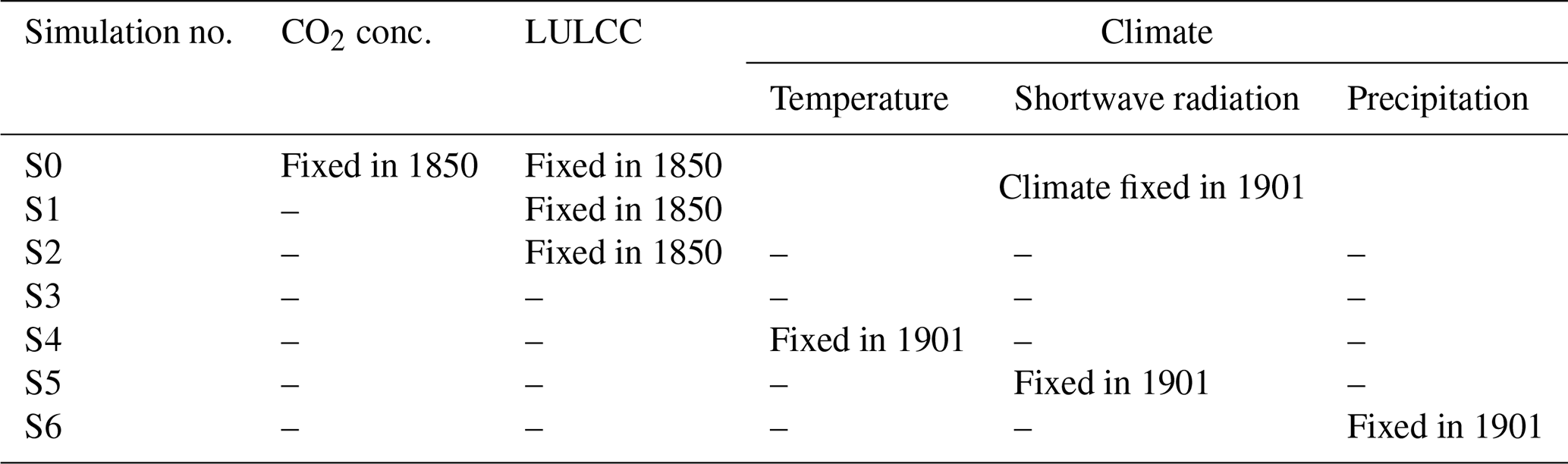
“–” denotes a variable that varied annually during the simulation period.

2.2 CMIP6 data

2.2.1 Model description

We analysed data obtained from the historical experiment in which all forcings (e.g. greenhouse gases (GHGs), aerosols, land use, solar, volcanic aerosols) evolved during 1850–2014 (Eyring et al., 2016). Relevant to this work, the external forcings for those simulations included land use change data originating from LUH2 (Hurtt et al., 2020), anthropogenic emissions from CEDS (Hoesly et al., 2018), and biomass burning emissions from BB4CMIP (van Marle et al., 2017). Five ESMs from CMIP6 were selected for their online BVOC emission schemes, including isoprene, but other ESMs use prescribed (interannually fixed) BVOC emissions (Gomez et al., 2023). Among the five selected ESMs, four used the empirically based Guenther scheme for isoprene estimation, albeit using different versions: CESM2-WACCM and NorESM2-LM share the same land component (Community Land Model – CLM5), employing the latest version of MEGAN, MEGANv2.1 (G2012) (Guenther et al., 2012), whereas GFDL-ESM4 and GISS-E2.1-G rely on earlier versions (G2006 and G1995, respectively) (Guenther et al., 1995, 2006). It is noteworthy that UKESM1-0-LL adopted the distinct photosynthesis-based iBVOC scheme (P2011) (Pacifico et al., 2011) to estimate isoprene emissions based on temperature, CO₂ concentration, and GPP. iBVOC in UKESM1-0-LL is derived from the Arneth et al. (2007b) and Niinemets et al. (1999) models, linking photosynthesis-derived electrons to the isoprene production rate, which is light-dependent. Because UKESM1-0-LL does not simulate electron transport directly, GPP is used as an approximation. Temperature and CO₂ inhibition effects are included empirically, accounting for differences in temperature optima and CO₂ responses between photosynthesis and isoprene synthesis. Table 2 presents simplified equations of isoprene emission schemes. Table S1 in the Supplement presents descriptions of symbols and parameters. Detailed model descriptions of other related processes are available elsewhere in the literature (Bauer et al., 2020; Emmons et al., 2020; Horowitz et al., 2020; Seland et al., 2020; Sellar et al., 2019).

Generally speaking, temperature and shortwave radiation enhance isoprene emissions in all models despite their differing component structures (Cao et al., 2021). Precipitation effects are represented either by the soil moisture factor in MEGAN (e.g. NorESM2-LM(G2012)) or indirectly through photosynthesis (GPP) in the UKESM1-0-LL(P2011) model (Clark et al., 2011). The influence of CO₂ on isoprene emissions varies across models. GFDL-ESM4(G2006) and GISS-E2.1-G(G1995) neglect both direct CO₂ inhibition and indirect fertilization effects because of prescribed satellite LAI (Horowitz et al., 2020; Ito et al., 2020). Also, CESM2-WACCM(G2012) and NorESM2-LM(G2012) use direct CO₂ inhibition effect parameterization from Heald et al. (2009), whereas UKESM1-0-LL(P2011) uses the scheme from Arneth et al. (2007b). The latter three models also incorporate indirect CO₂ fertilization effects through vegetation growth and terrestrial carbon processes, influencing LAI or GPP.

Table 2 Summary of CMIP6 models and their simplified isoprene emission schemes.

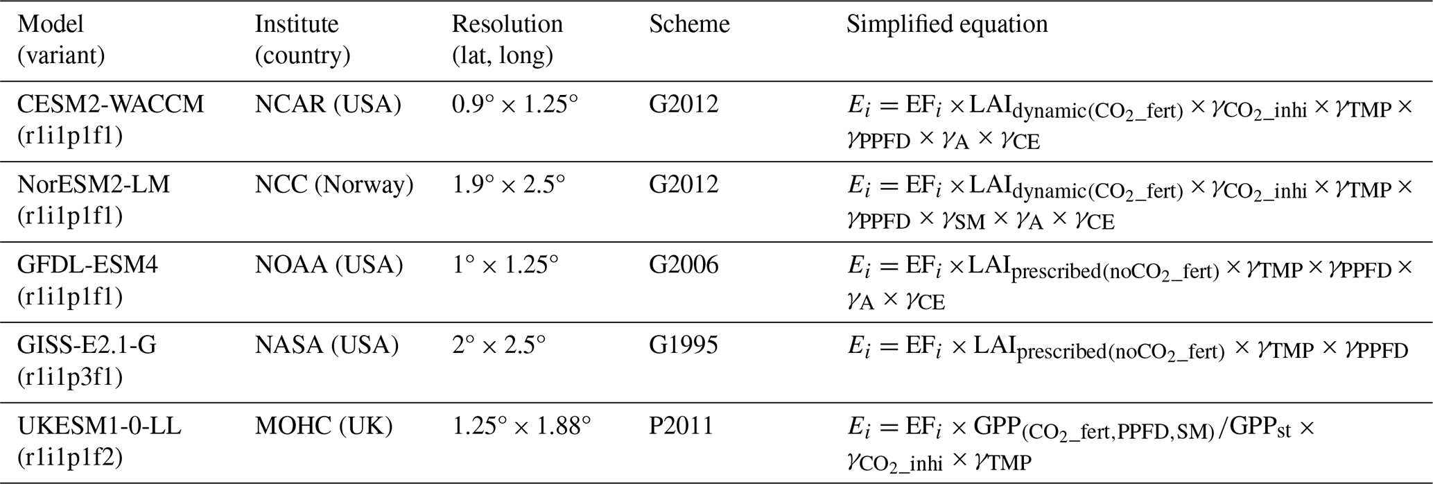
E_i is the isoprene emission rate. EF_i is the isoprene emission factor applied for each PFT under standard conditions. ${\mathrm{LAI}}_{\mathrm{dynamic}\left({\mathrm{CO}}_{\mathrm{2}}\mathrm{\_}\mathrm{fert}\right)}$ is the leaf area index updated in response to increasing CO₂ concentration via photosynthesis (CO₂ fertilization effect). ${\mathrm{LAI}}_{\mathrm{prescribed}\left({\mathrm{noCO}}_{\mathrm{2}}\mathrm{\_}\mathrm{fert}\right)}$ is the prescribed satellite leaf area index which does not consider CO₂ fertilization effect. GPP denotes gross primary productivity, updated in response to increasing CO₂ concentration via photosynthesis (CO₂ fertilization effect), light, and soil moisture. “st” represents standard conditions. ${\mathit{\gamma }}_{{\mathrm{CO}}_{\mathrm{2}}\mathrm{\_}\mathrm{inhi}}$, γ_TMP, γ_PPFD, γ_SM, γ_A, and γ_CE stand for activity factors representing the CO₂ inhibition effect and dependence of isoprene emissions caused by temperature, light (photosynthetic photon flux density), soil moisture, leaf age, and the canopy environment, respectively. Detailed descriptions of symbols and parameters in the isoprene emission equations are presented in Table S1.

2.2.2 Emulation of isoprene emissions

Understanding the complex influences on isoprene emissions requires analyses of various factors. The initial step is to reproduce isoprene emissions for each ESM accurately based on key input factors including atmospheric CO₂ concentration, LULCC, and climate variables. To accomplish this step, we developed a data-driven regression model using a machine learning approach to estimate annual isoprene emissions based on critical drivers within ESMs. For each ESM, the features input into the regression model include the same drivers for isoprene emission simulation used in the CMIP6 project. For models that are sensitive to CO₂ (CESM2-WACCM(G2012), NorESM2-LM(G2012), UKESM1-0-LL(P2011)), the features comprise CO₂; LULCC (represented by the tree fraction); and climate variables such as temperature (tas), surface downwelling shortwave radiation (rsds; hereafter referred to as shortwave radiation), and precipitation (pr). For those models which are not sensitive to CO₂ (GFDL-ESM4(G2006) and GISS-E2.1-G(G1995)), the features only include LULCC and climate variables. We chose random forest as the machine learning algorithm to build regression models because of its ability to handle complex, nonlinear relations among variables without requiring assumptions (Guo et al., 2015; Zhang et al., 2017).

To assess the regression model performance, we used a threefold cross-validation approach. The dataset was divided into three periods: 1850–1904 (fold 1), 1905–1959 (fold 2), and 1960–2014 (fold 3). During each iteration, one fold was designated as the test set, whereas the remaining two folds were used for training the model. The evaluation metrics included the coefficient of determination (R²), root mean squared error (RMSE), and mean absolute error (MAE). The results of the threefold cross-validation for each ESM are presented in Fig. S1 in the Supplement, in which the models exhibited high R² values (>0.9) and low errors across all ESMs during cross-validation. Furthermore, the estimated historical trend of global annual isoprene emission using random forest showed strong correlation (r>0.9) and consistency with the CMIP6 simulation for all ESMs (Fig. S2). These results demonstrate that the random forest models perform well in reproducing isoprene emissions for all CMIP6 models based on the selected variables.

For further identification of the individual effects of each driver on isoprene emissions, we used random forest regression as an emulator to replicate sensitivity experiments for each CMIP6 model. This method involved generation of isoprene emissions using the trained random forest regressor with varied settings for the input drivers for each CMIP6 ESM, as outlined in Tables S2 and S3. First, to investigate the effects of CO₂, LULCC, and climate on isoprene emissions, we emulated sensitivity experiments (S0–S3) similar to those conducted using the VISIT(G1997) model for CO₂-sensitive models including CESM2-WACCM(G2012), NorESM2-LM(G2012), and UKESM1-0-LL(P2011). For the other two models, GFDL-ESM4(G2006) and GISS-E2.1-G(G1995), we modified the experiments (S1^′–S3^′) to compare the LULCC and climate effects. Subsequently, to identify the main climate drivers (temperature, shortwave radiation, and precipitation) of isoprene emissions, we conducted three additional simulations similar to S4–S6 of VISIT(G1997). Detailed descriptions of these experiments are presented in Tables S2 and S3.

All historical simulation data (including isoprene emissions and other relevant variables described above) for each model were downloaded via the Earth System Grid Federation portal (ESGF, 2023). To facilitate comparison, we resampled spatial resolutions of different models to a consistent 1° × 1.25° grid and calculated annual values before analysis.

2.3 Analysis methods

2.3.1 Attributions of isoprene emission changes

To isolate the effects of CO₂, LULCC, and climate on isoprene emissions, four simulations (S0, S1, S2, and S3) were conducted for VISIT(G1997) and CMIP6 models to consider the CO₂ effects (CESM2-WACCM(G2012), NorESM2-LM(G2012), and UKESM1-0-LL(P2011)). Although VISIT only incorporates the CO₂ fertilization effect (increase) via LAI/GPP, these CMIP6 models also account for the direct CO₂ inhibition effect (decrease) on isoprene emissions. Consequently, in VISIT, the CO₂ effects on isoprene emissions are attributable to fertilization only. By contrast, in these CMIP6 models, the net effect of both fertilization and inhibition effects is included. The effects were calculated by comparing isoprene emission simulations with fixed and varied states for each driver: the CO₂ effect (difference in isoprene emissions between S1 and S0, S1 − S0), the LULCC effect (S3 − S2), the climate effect (S2 − S1), and three combined drivers (S3 − S0). For models without the CO₂ effects, GFDL-ESM4(G2006) and GISS-E2.1-G(G1995), three simulations (S1^′, S2^′, and S3^′) were used, with effects calculated as the LULCC effect (S3^′ − S2^′), climate effect (S2^′ − S1^′), and two combined drivers (S3^′ − S1^′).

Finally, to identify individual climate driver effects (temperature, shortwave radiation, and precipitation), we compared S3 (all varied) with three additional fixed-case simulations (S4, S5, and S6): the temperature effect (S3 − S4), the radiation effect (S3 − S5), and the precipitation effect (S3 − S6).

2.3.2 Significance test for long-term trends of isoprene emissions

We performed the Mann–Kendall trends test (Kendall, 1975; Mann, 1945) and the Theil–Sen estimator (Sen, 1968; Theil, 1950) to detect robust trends in annual isoprene emissions and their attributing factors (i.e. the effects of CO₂, LULCC, and climate (temperature, radiation, and precipitation)) for each model at global and grid scales. The Mann–Kendall test, a nonparametric method for trend analysis, has been employed widely for analysing hydrometeorological and biogeochemical time series (Kondo et al., 2018; Pan et al., 2020; Yue and Wang, 2004). The Theil–Sen method was used to calculate the magnitude of the trend. The Mann–Kendall test was used to determine the significance level (p<0.05) of the trends in isoprene emissions.

At a global scale, trend tests were conducted for 1850–2014, 1850–1979, and 1980–2014, applied to global annual totals of isoprene emission and global means of climate variables from historical simulation of CMIP6 models and VISIT-S3(G1997) over land area (Table 3). At the grid scale, similar trend tests were applied for 1850–2014 to annual totals of isoprene emissions (Fig. 5) and to annual means of climate variables from historical simulation of CMIP6 models and VISIT-S3(G1997) (Fig. S7).

To identify trends in contributing factors to global isoprene emissions (1850–2014), we used the effects of CO₂, LULCC, climate, and individual climate drivers (as presented in Sect. 2.3.1) from CMIP6 and VISIT(G1997) model simulations. Trend tests were then applied to individual model outputs (Figs. 7 and 9). For grid-scale trends (1850–2014), we applied trend tests to annual isoprene emissions from the effects of each driver (CO₂, LULCC, and climate) (Fig. 10). The driver with the absolute most prominent isoprene emission trend was identified as the dominant driver (Fig. 11). Similarly, to identify the main climate driver for grid-scale trends (1850–2014), we applied the trend test to annual isoprene emissions induced by each climate driver (Fig. 12). The climate factor with the absolute most prominent isoprene emission trend was then identified as the dominant climate driver (Fig. 13).

3 Results

3.1 Global and regional isoprene emissions in the present day

The mean annual global isoprene emissions during 2000–2014 agreed well with results obtained using VISIT-S3(G1997) simulation and CMIP6 models, at 434–510 TgC yr⁻¹ (Fig. 1a). GFDL-ESM4(G2006) stands at the lower end with 434 TgC yr⁻¹, whereas VISIT-S3(G1997) offers the highest estimate at 510 TgC yr⁻¹. These values fall within the broader range of 308–705 TgC yr⁻¹ (equivalent to 350–800 Tg yr⁻¹) described in reports of earlier studies using stand-alone MEGAN models with diverse weather and land cover data for 2000 (Guenther et al., 2012). Recent studies using an empirical approach with MEGANv2.1(G2012) further support this range, estimating the mean annual global isoprene emissions for the present day as 370–524 TgC yr⁻¹. Examples include 370 TgC yr⁻¹ for MEGAN-MOHYCAN covering 2000–2016 (Opacka et al., 2021), 388 TgC yr⁻¹ for CAMS-GLOB-BIOv3.1 over 2000–2019 (Sindelarova et al., 2022), and 524 TgC yr⁻¹ for MEGAN-MACC during 1980–2010 (Sindelarova et al., 2014). It is noteworthy that all these datasets except MEGAN-MACC neglected the effects of CO₂ inhibition and soil moisture, which MEGAN-MACC does account for (Sindelarova et al., 2014). Earlier studies using a photosynthesis-based approach also reported diverse estimates of global isoprene emissions, with values of 516–522 TgC yr⁻¹ for 1990–1999 (Pacifico et al., 2011) and 463 TgC yr⁻¹ for 1981–2002 (Arneth et al., 2011). In this study's present day (2000–2014), the UKESM1-0-LL(P2011) isoprene emission of 478 TgC yr⁻¹ aligns with the range of these earlier studies.

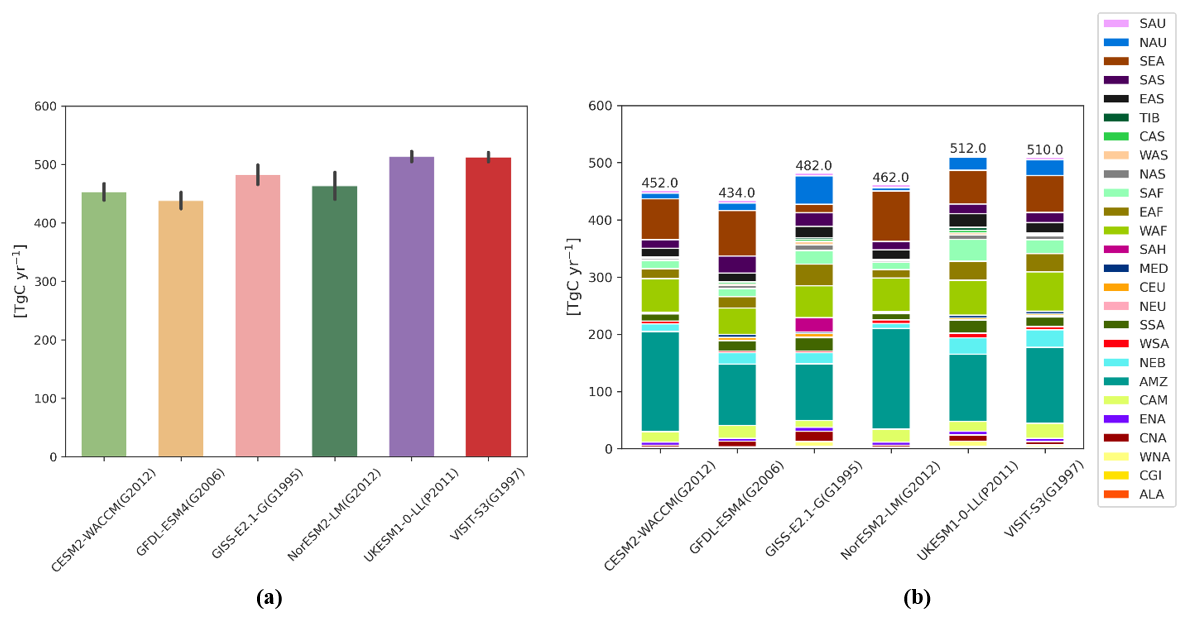
Figure 1 Mean annual (a) global and (b) regional isoprene emissions in the present day (2000–2014). Error bars in (a) represent the standard deviation for each model. The top of (b) portrays the absolute contributions of 26 regions to global totals. These regions correspond to the 26 SREX regions defined by the IPCC Special Report called Managing the Risks of Extreme Events and Disasters to Advance Climate Change Adaptation (Seneviratne et al., 2012), as shown in Fig. S3. The colour bar on the right shows the colours assigned to the respective regions.

Although CMIP6 models and VISIT-S3(G1997) simulation agreed well in terms of the mean annual global isoprene emissions over 2000–2014, pronounced differences were found for regional emissions, as presented in Fig. 1b and in Table S4. The tropics dominate isoprene emissions across all models, but the contribution varies considerably. The mean annual emissions for tropical regions including the Amazon (AMZ), West Africa (WAF), East Africa (EAF), and Southeast Asia (SEA), are 207–377 TgC yr⁻¹, representing 43 % to 73 % of global isoprene emissions for GISS-E2.1-G(G1995) and CESM2-WACCM(G2012)/NorESM2-LM(G2012). Other models estimate a similar tropical dominance, exceeding 50 % of global totals.

Considerable uncertainties were found for tropical isoprene emissions, particularly in the Amazon. Model-derived estimates vary from 98 TgC yr⁻¹ in GISS-E2.1-G(G1995) to 175 TgC yr⁻¹ in CESM2-WACCM(G2012) and NorESM2-LM(G2012). Similarly, Southeast Asia displays wide variation, with GISS-E2.1-G(G1995) and NorESM2-LM(G2012) estimated as 14.7–87.8 TgC yr⁻¹. However, West Africa (WAF) shows less variation, with model estimates ranging from 45.5–68.6 TgC yr⁻¹ and GFDL-ESM4(G2006) offering the lowest estimate.

Arid and semiarid regions display the highest variability in isoprene emission estimates. For instance, GISS-E2.1-G(G1995) attributes considerably higher emissions to the Sahara (SAH) (24.9 TgC yr⁻¹) than other models do (0.1–4.3 TgC yr⁻¹). Similarly, in northern Australia (NAU), GISS-E2.1-G(G1995) estimates emissions of 49.8 TgC yr⁻¹, which is approximately 2–7 times higher than those estimates of other models (6.4–27.5 TgC yr⁻¹). Furthermore, isoprene emissions remain consistent across models in eastern North America (ENA) (5.1–6.7 TgC yr⁻¹) and East Asia (EAS) (15.2–21.6 TgC yr⁻¹). For northeastern Brazil (NEB), VISIT-S3(G1997) calculates an emission of 30.9 TgC yr⁻¹, which is closely aligned with UKESM1-0-LL(P2011)'s estimate of 27.67 TgC yr⁻¹ but exceeds those estimates in other models (8.7–13.2 TgC yr⁻¹).

Across all models, isoprene emissions exhibit an apparent decline from warm and humid tropical forests towards colder and drier biomes such as tundra and deserts, as presented in Fig. 2. However, large discrepancies are apparent between model estimates in tropical regions (the Amazon, equatorial Africa, and Southeast Asia). The Amazon consistently stands out as the region with the highest isoprene emissions across all models, but the magnitude of this emission varies considerably. The CESM2-WACCM(G2012) and NorESM2-LM(G2012) models simulate intense emissions, with the central Amazon showing the highest values. VISIT-S3(G1997) and UKESM1-0-LL(P2011) also identify the central Amazon as an emission hotspot but show relatively high emissions in the northwestern Amazon. This pattern aligns with satellite retrievals of isoprene concentrations over this region (Wells et al., 2022), though the emissions are of a smaller magnitude compared to those simulated by CESM2-WACCM(G2012) and NorESM2-LM(G2012). However, the GFDL-ESM4(G2006) and GISS-E2.1-G(G1995) models recognize the western Amazon and northern Amazon as emission hotspots, respectively, although these signals are weaker compared to in other models. Equatorial Africa, including West Africa (WAF) and East Africa (EAF), presents a contrasting scenario. Actually, GISS-E2.1-G(G1995) suggests a broader area of high emission, but other models concentrate this peak around 20° E. The spatial emission pattern in Southeast Asia remains consistent across models, but CESM2-WACCM(G2012) and NorESM2-LM(G2012) show higher values. Low emission estimates consistently characterize high northern latitudes (e.g. Alaska (ALA); Canada, Greenland, and Iceland (CGI)) and arid–semiarid regions such as Central Asia (CAS), western North America (WNA), and the Sahara (SAH). Northern Australia (NAU) is a notable exception, with GISS-E2.1-G(G1995) estimating much higher emissions than other models, which offer consistently low values.

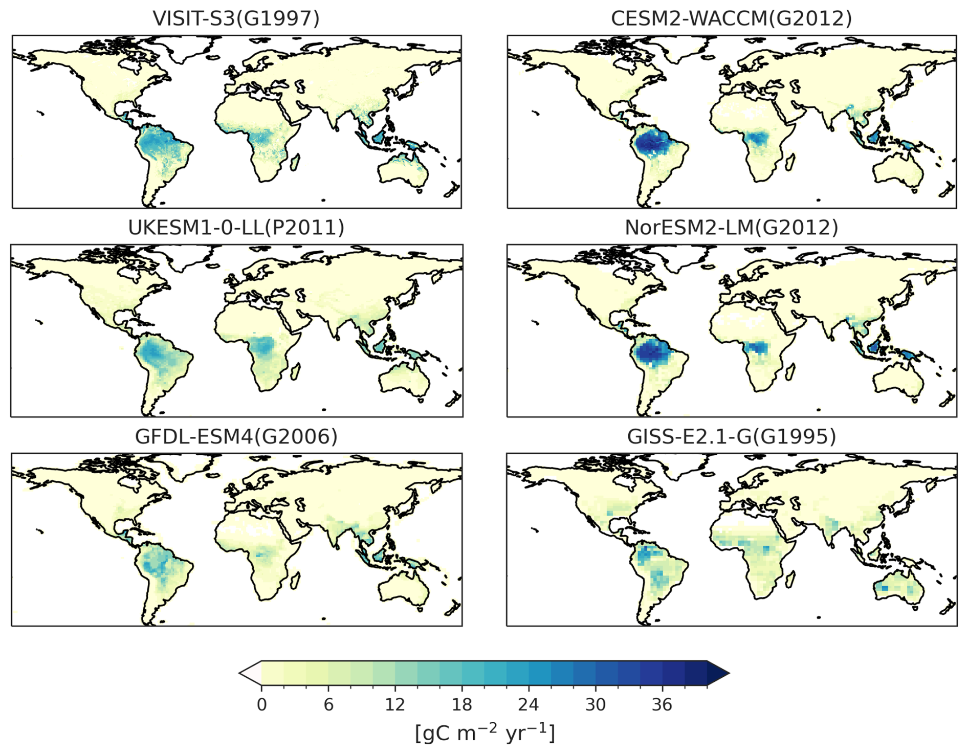
Figure 2 Spatial distributions of mean annual isoprene emissions in the present day (2000–2014).

As presented in Fig. 3, the latitudinal profiles of isoprene emissions reveal general agreement among models, with a single peak around the Equator. The exception is GISS-E2.1-G(G1995), which exhibits a second peak around −25° S, coinciding with high emissions in Australia. Two models, CESM2-WACCM(G2012) and NorESM2-LM(G2012) stand out for their steeper spatial gradient, particularly between the tropics and other regions, showing lower emissions at high latitudes and higher emissions in the tropics than other models do. A considerable degree of uncertainty prevails within the tropics, with the highest and lowest estimates differing nearly 2-fold. CESM2-WACCM(G2012) and NorESM2-LM(G2012) estimate the highest emissions, exceeding 4 gC m⁻² yr⁻¹, whereas GISS-E2.1-G(G1995) estimates much lower values below 2.5 gC m⁻²yr⁻¹. VISIT-S3(G1997) and UKESM1-0-LL(P2011) occupy the middle range, with estimates of approximately 3 gC m⁻² yr⁻¹. The primary reason underlying variation in the regional distribution of isoprene emissions among models likely stems from discrepancies in vegetation distribution and emission factors, as elaborated in Sect. 4.1.1.

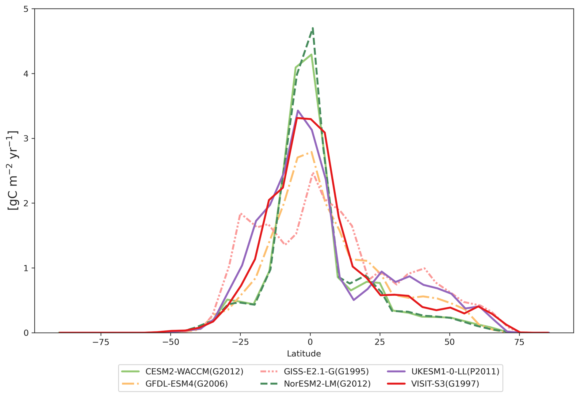
Figure 3 Latitudinal profiles of mean annual isoprene emissions in the present day (2000–2014).

3.2 Long-term trends of global isoprene emissions

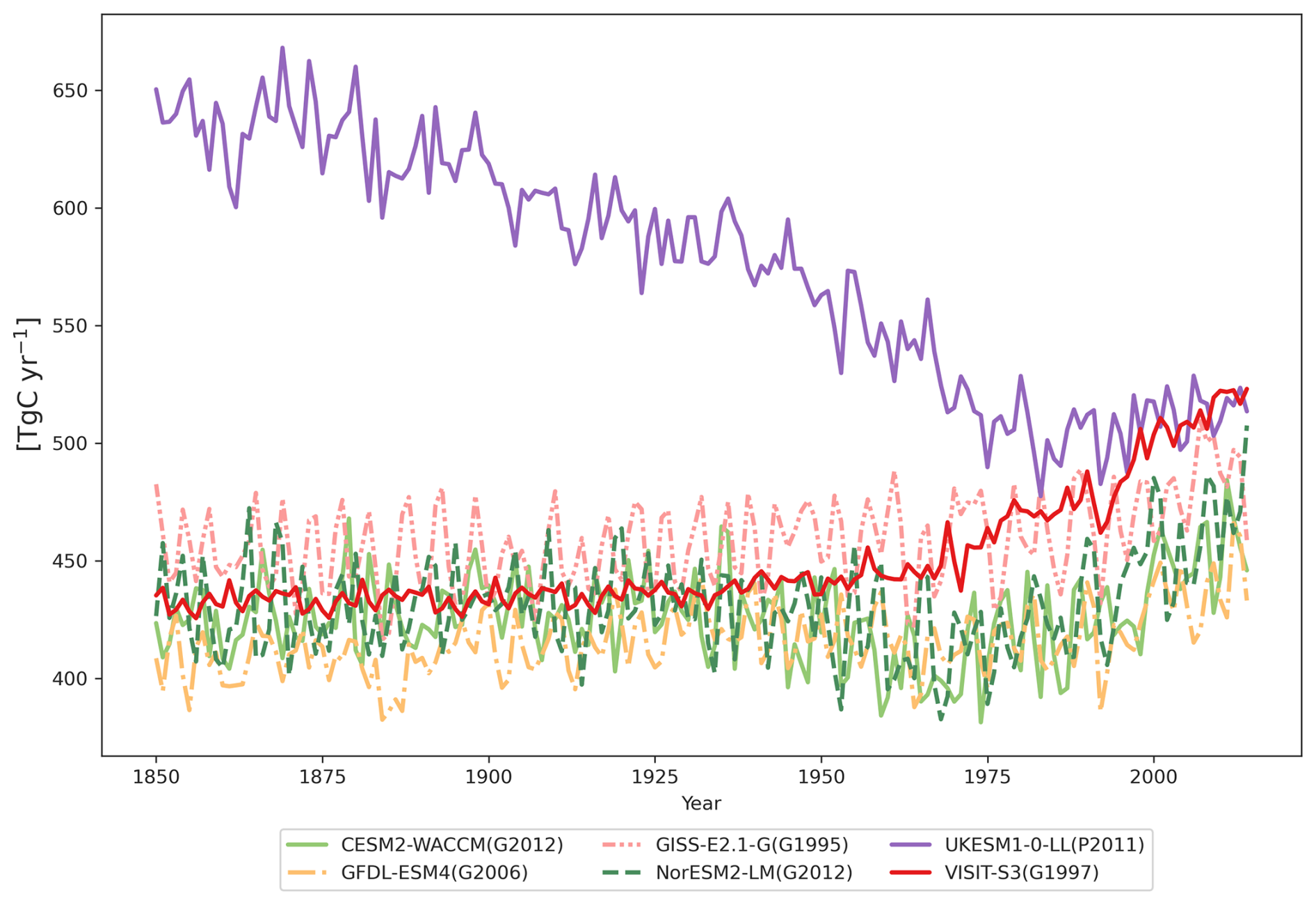
Considerable uncertainty surrounds global isoprene emission trends throughout 1850–2014 (Table 3 and Fig. 4). While three models (VISIT-S3(G1997), GFDL-ESM4(G2006), and GISS-E2.1-G(G1995)) show an upward trend (+0.13 to +0.31 TgC yr⁻²), CESM2-WACCM(G2012) and NorESM2-LM(G2012) find no significant trend. In contrast, UKESM1-0-LL(P2011) exhibits a decline in global isoprene emissions at a rate of −0.92 TgC yr⁻². Despite these differences in isoprene emission trends, all models show that temperature increases consistently: +0.002 to +0.005 °C yr⁻¹.

Table 3 Global isoprene emission and temperature trends over three periods: 1850–2014, 1850–1979, and 1980–2014. Bold values indicate that a trend is significant, with p<0.05.

Figure 4 Interannual variations in global isoprene emissions during 1850–2014.

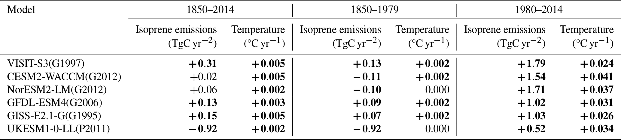
From preindustrial times to 1980 includes a period of considerable uncertainty in isoprene emissions, despite most models using similar algorithms, except UKESM1-0-LL(P2011) (Table 2). Three models (CESM2-WACCM(G2012), NorESM2-LM(G2012), and UKESM1-0-LL(P2011)) show a significant decrease (p<0.05), with UKESM1-0-LL(P2011) experiencing the largest decline of −0.92 TgC yr⁻² compared to a −0.11 TgC yr⁻² decrease in the other two models. Conversely, GFDL-ESM4(G2006), GISS-E2.1-G(G1995), and VISIT-S3(G1997) show significant increases (+0.07 to +0.13 TgC yr⁻²). For temperature, except for NorESM2-LM(G2012) and UKESM1-0-LL(P2011), which revealed no significant trend, the other models exhibited a significant and moderate trend of +0.002 °C yr⁻¹ for this period (1850–1979).

From 1980–2014, all models show significantly increasing trends in global isoprene emissions, but their magnitudes vary (1.27 ± 0.49 TgC yr⁻², 0.28 ± 0.11 % yr⁻¹). Specifically, VISIT-S3(G1997) projects the largest increase (+1.79 TgC yr⁻²), followed by NorESM2-LM(G2012) and CESM2-WACCM(G2012) (+1.71 and +1.54 TgC yr⁻², respectively). GFDL-ESM4(G2006) and GISS-E2.1-G(G1995) show moderate increases (+1.02 and +1.03 TgC yr⁻², respectively), whereas UKESM1-0-LL(P2011) shows the smallest increase (+0.52 TgC yr⁻²). In contrast, this period (1980–2014) showed a similar increase in global temperature for all models, of +0.024 to +0.041 °C yr⁻¹ (p<0.05) among all models. The remarkable rise in temperature during this period can likely be attributed to the surge in GHG concentrations, particularly CO₂, and the decline in aerosol levels relative to the preceding period (1850–1979). It is particularly interesting that among models using the Guenther scheme, those with both CO₂ effects (CESM2-WACCM(G2012), NorESM2-LM(G2012)) and CO₂ fertilization only (VISIT-S3(G1997)) exhibit more positive trends in isoprene emissions than in models without CO₂ effects. This predominance of positive trends implies that, in addition to increasing temperature, CO₂ fertilization might be the second most important factor contributing to the marked increases in isoprene emission simulated in these models. For UKESM1-0-LL(P2011), even though its temperature trend is similar to other models, the smaller increase in isoprene emissions compared to those found using other Guenther-based models might be explained by its different scheme, which we investigate and discuss as presented hereinafter.

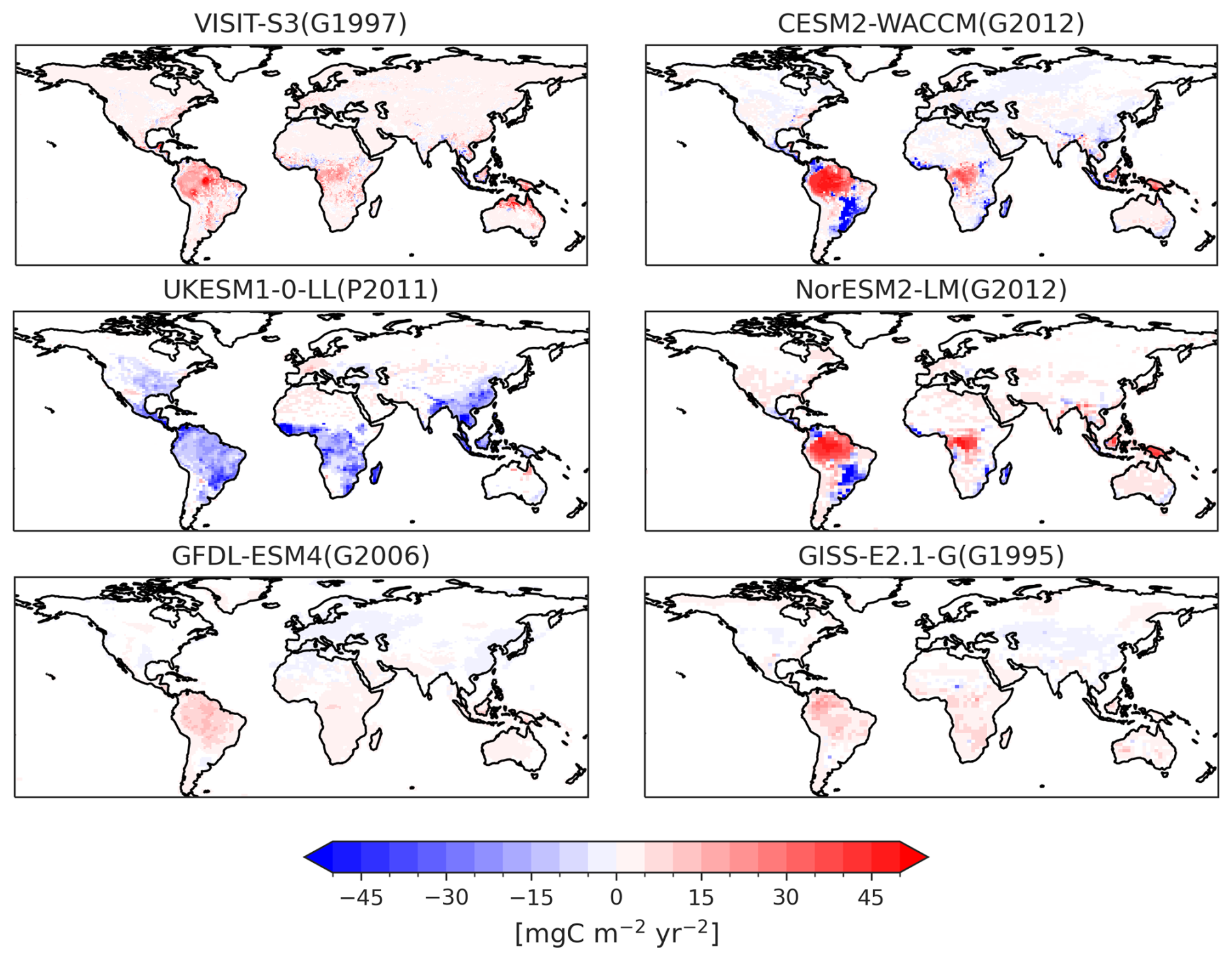
Figure 5 Spatial distribution of isoprene emission trends during 1850–2014. Only significant trends (with p<0.05) are presented.

Figure 5 reveals remarkable similarities in the spatial distribution of isoprene emission trends during 1850–2014 between CESM2-WACCM(G2012) and NorESM2-LM(G2012). These similarities are likely attributable to their shared land model (CLM5), which incorporates the same version of the isoprene emission scheme G2012, as well as a shared atmosphere model (CAM6), albeit with somewhat different parameterizations and tuning. This pattern diverges from those of other models. Notably, all models employing the Guenther scheme agree on marked increases in specific regions such as the Amazon and central Africa, although these trends differ in terms of magnitude. Discrepancies emerge primarily in other regions. In South America and southern Africa, GISS-E2.1-G(G1995), VISIT-S3(G1997), and GFDL-ESM4(G2006) project a wider area of rising isoprene emission, whereas CESM2-WACCM(G2012), NorESM2-LM(G2012), and UKESM1-0-LL(P2011) suggest a larger area of decline. UKESM1-0-LL(P2011) exhibits a decrease in most regions, except in parts of western North America (WNA) and central Europe (CEU). Furthermore, high-latitude regions (north of 60° N) were found to have no significant trends in isoprene emissions in CESM2-WACCM(G2012), NorESM2-LM(G2012), GFDL-ESM4(G2006), and GISS-E2.1-G(G1995). By contrast, UKESM1-0-LL(P2011) projects a considerable decrease, whereas VISIT-S3(G1997) shows an increase in these regions.

3.3 Contribution of drivers to global isoprene emission changes

Elevated CO₂, LULCC, and climate effects on annual global isoprene emission changes in individual models during 1850–2014 are shown in Fig. 6. Figure 7 presents a comparison of these trends during 1850–2014. The models including CO₂ effects indicated that most of the long-term trends in isoprene emissions can be attributed to CO₂ and LULCC. Four models consistently project a gradual decrease in emissions because of LULCC from 1850, although the magnitudes vary. CESM2-WACCM(G2012) shows the largest decrease (−0.42 TgC yr⁻²), followed closely by NorESM2-LM(G2012), UKESM1-0-LL(P2011), and VISIT(G1997) (−0.27, −0.24, and −0.23 TgC yr⁻², respectively). However, the CO₂ effect here, representing the net total effects of fertilization (increase) and inhibition (decrease), remains highly uncertain. While VISIT(G1997), CESM2-WACCM(G2012), and NorESM2-LM(G2012) show positive effects (+0.42, +0.36, and +0.26 TgC yr⁻², respectively), UKESM1-0-LL(P2011) exhibits a negative effect of CO₂ on the isoprene long-term emission trend (−0.61 TgC yr⁻²). The underlying source of uncertainty related to these divergent trends among the models is discussed in Sect. 4.1.3. Although climate exerts a slight effect on long-term trends in isoprene emissions, it influences interannual variation within this model group. In contrast, GFDL-ESM4(G2006) and GISS-E2.1-G(G1995), excluding the CO₂ effects, attribute long-term emission trends primarily to climate (+0.12 and +0.15 TgC yr⁻², respectively), with LULCC playing a negligible role (−0.0005 TgC yr⁻²).

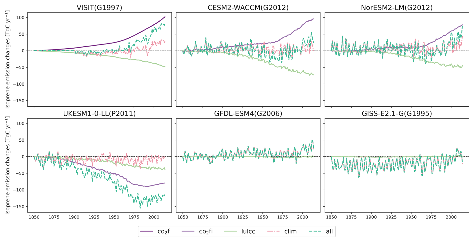
Figure 6 Effects of drivers on global isoprene emissions during 1850–2014: CO₂ (co₂f, CO₂ fertilization only; co₂fi, combined CO₂ fertilization and inhibition), land use and land cover change (lulcc), climate (clim), and the combination of three drivers (all). These effects were calculated as the difference in isoprene emission simulations between fixed and varied states for each driver, details of which are described in Sect. 2.3.1.

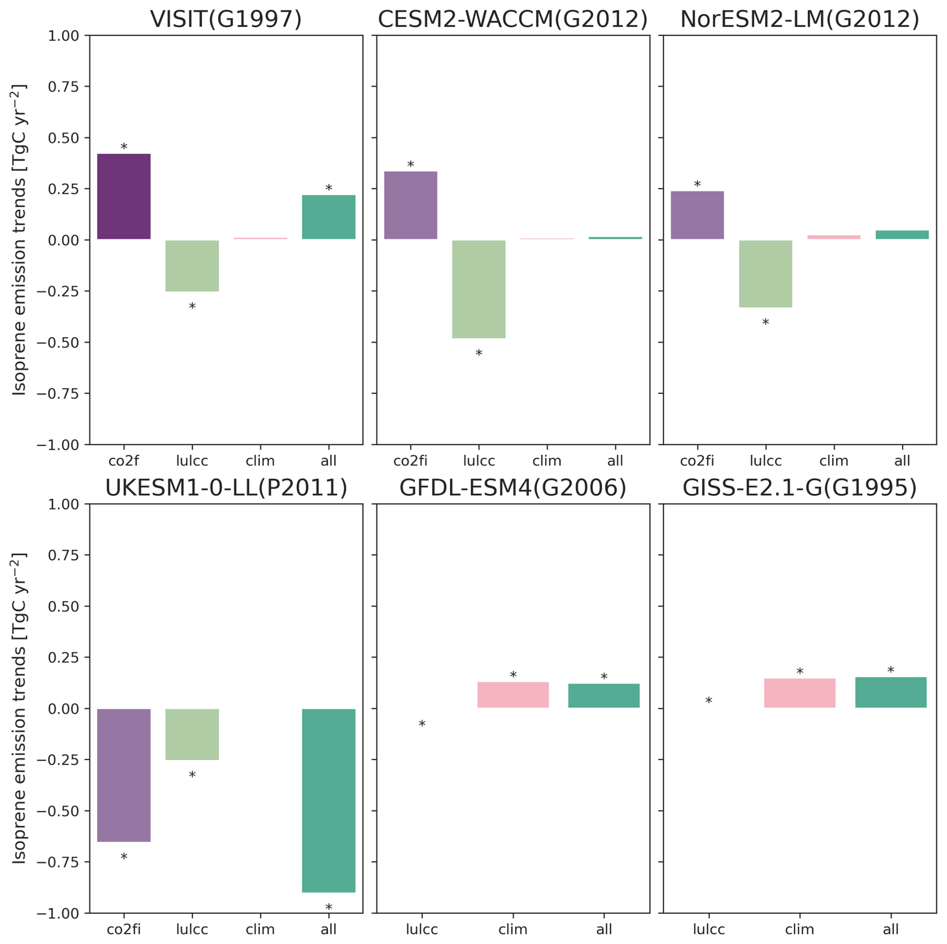
Figure 7 Attribution of global isoprene emission trends during 1850–2014 attributable to each driver (co₂f/co₂fi, lulcc, and clim) and the combination of three drivers (all). Asterisks denote a significant trend, with p<0.05.

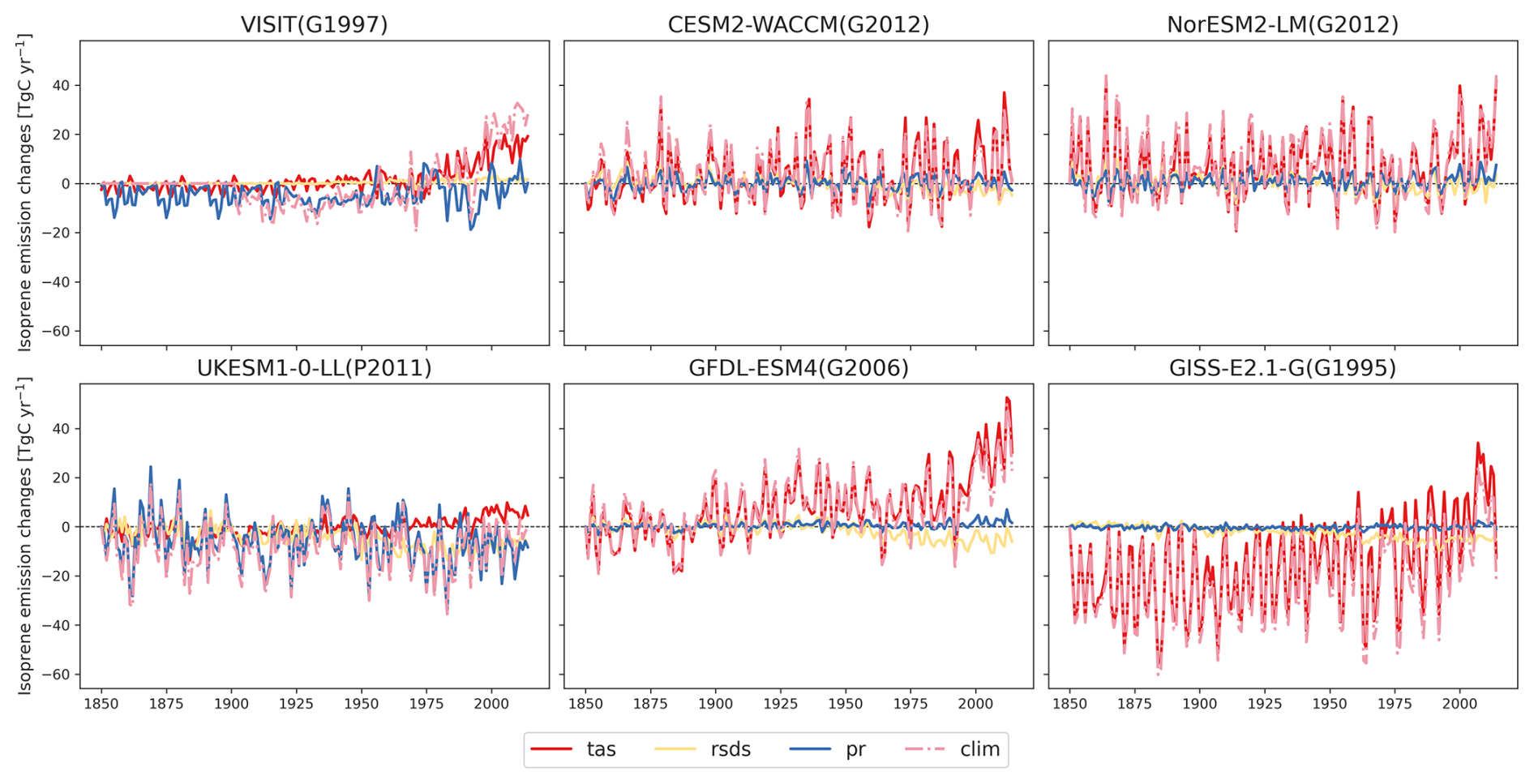
Figure 8 Effects of climate factors on global isoprene emissions during 1850–2014: temperature (tas), shortwave radiation (rsds), precipitation (pr), and total climate factors (clim).

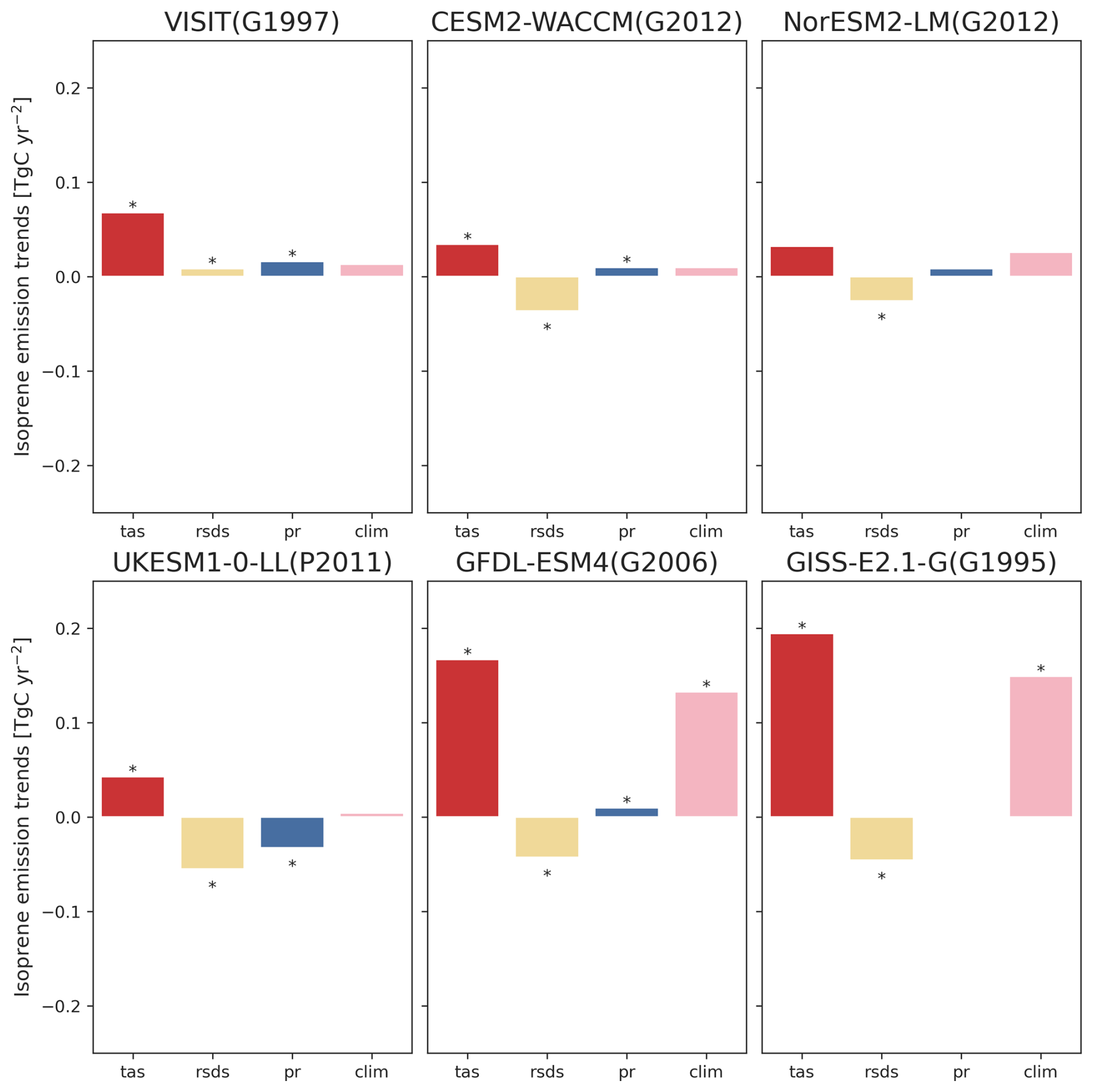
Figure 9 Attribution of global isoprene emission trends during 1850–2014 attributable to each climate factor (tas, rsds, pr) and total climate effects (clim). Asterisks denote a significant trend, with p<0.05.

Figures 8 and 9 present individual climate factors influencing the isoprene emission trends. Climate is a strong driver of year-to-year variation in isoprene emissions in all models, with the most decisive influence in GFDL-ESM4(G2006) and GISS-E2.1-G(G1995). Empirically based CMIP6 models agree that temperature is the primary driver of interannual variation in isoprene emissions, whereas the photosynthesis-based model UKESM1-0-LL(P2011) highlights radiation and precipitation and VISIT(G1997) emphasizes temperature and precipitation over radiation (Fig. 8). Interannual variations in these climate variables primarily drive interannual changes in isoprene emissions across models. VISIT(G1997) notably exhibits lower interannual variation in isoprene emissions than that in the CMIP6 models, primarily because it relies on reanalysis climate data, which contain less variability compared to the climate data simulated by the CMIP6 models (Fig. S5 and Table S5). The small interannual variability during 1850–1900 simulated by VISIT could come from the spin-up method using climatological forcing data, with the model being repeatedly driven by the climate data of 1901 during this period. Furthermore, although GISS-E2.1-G(G1995) uses a temperature-dependent algorithm similar to that of VISIT(G1997) (Table S1), the greater temperature variability in GISS-E2.1-G(G1995) results in larger interannual variation in isoprene emissions. Regarding long-term trends, climate factors exert a stronger influence on emission trends in GFDL-ESM4(G2006) and GISS-E2.1-G(G1995) compared to the other models. All models show agreement on temperature-increasing isoprene emission, but the specific effects vary: +0.04 to +0.18 TgC yr⁻². However, the VISIT(G1997) model reveals that radiation causes only a minor increase (+0.005 TgC yr⁻², p>0.05). In contrast, CMIP6 models indicate that decreased radiation contributes to a minor reduction in isoprene emission, ranging from −0.02 to −0.04 TgC yr⁻² (p<0.05). The effects of precipitation further highlight discrepancies among models: VISIT(G1997) shows an increase in emissions (+0.02 TgC yr⁻²), whereas UKESM1-0-LL(P2011) projects a decrease (−0.04 TgC yr⁻²), and other models show non-significant trends (+0.003 to +0.006 TgC yr⁻²) attributed to precipitation.

3.4 Spatial contribution of drivers when estimating isoprene emissions

Figure 10 shows that CO₂ and LULCC influence isoprene emission changes more than climate in the models including the CO₂ effect. CO₂ primarily drives increased emissions, especially in tropical regions, for VISIT(G1997), CESM2-WACCM(G2012), and NorESM2-LM(G2012), whereas UKESM1-0-LL(P2011) exhibits a decreasing trend. However, these models show agreement in that LULCC engenders decreasing emissions, particularly in regions such as central Africa and southern Africa, as well as South Asia and Southeast Asia. However, parts of Europe and eastern North America show increases. In southeastern South America (SSA), CESM2-WACCM(G2012), NorESM2-LM(G2012), and UKESM1-0-LL(P2011) (excluding VISIT(G1997)) identify LULCC (deforestation) as the main driver of emission changes. However, GFDL-ESM4(G2006) and GISS-E2.1-G(G1995), without CO₂ effects, find the LULCC effect on isoprene emission changes to be minimal compared to the other models. Regarding climate effects on isoprene emission, differences in climate variability explain the discrepancies in model contributions.

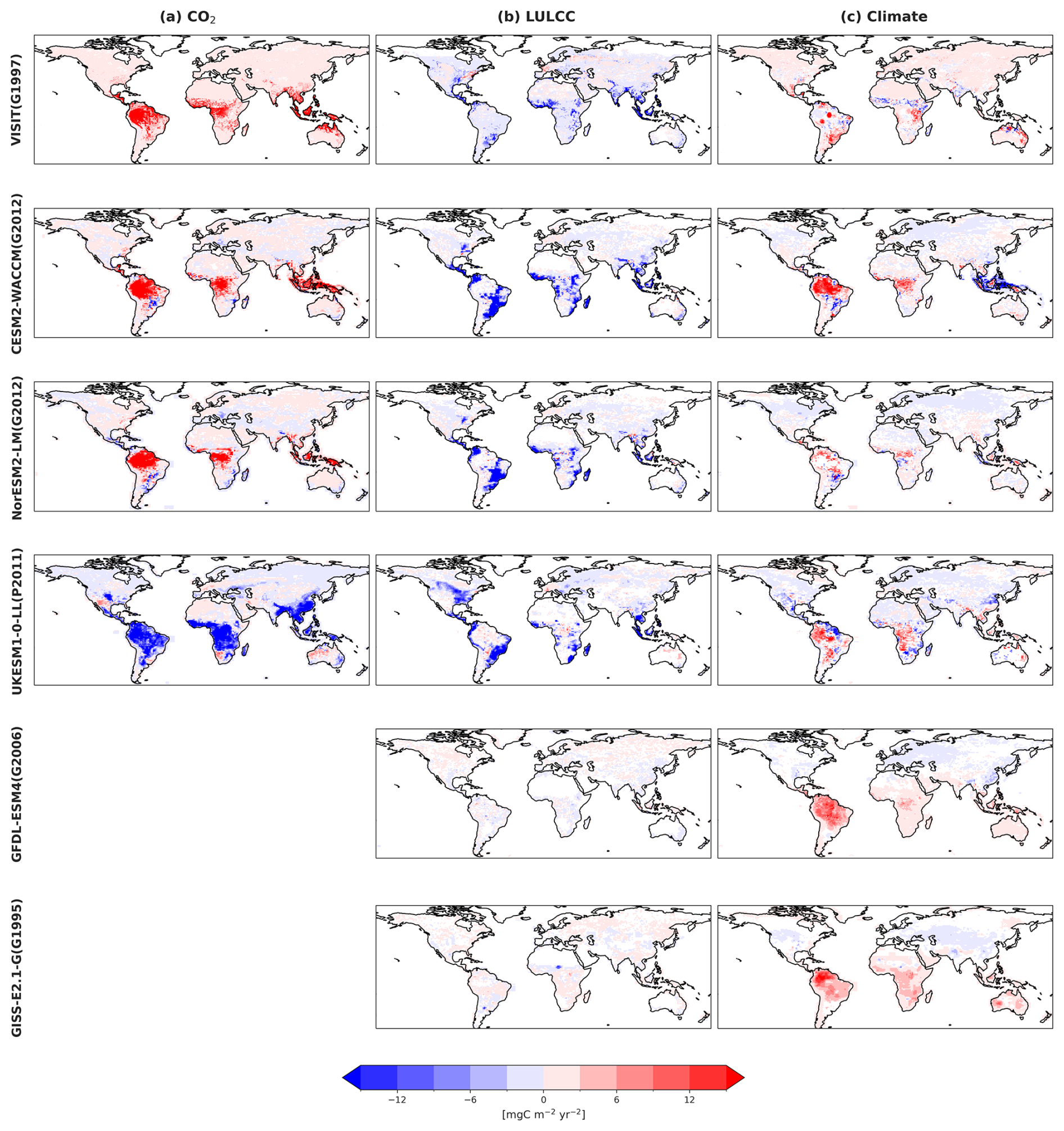
Figure 10 Spatial distributions of the contributions of (a) CO₂, (b) LULCC, and (c) climate to the isoprene emission trends in the respective models. Only significant trends (with p<0.05) are presented. It is noteworthy that GFDL-ESM4(G2006) and GISS-E2.1-G(G1995) do not include the CO₂ effects.

A spatial distribution of the most dominant variables influencing isoprene emission trends across CO₂, LULCC, and climate is portrayed in Fig. 11. Overall, CO₂ emerges as the dominant driver for 34 %–63 % of global land area in VISIT(G1997), CESM2-WACCM(G2012), NorESM2-LM(G2012), and UKESM1-0-LL(P2011). Here, LULCC plays a minor role, accounting for 14 %–25 % of the global land area in all models, but its spatial distribution of dominance varies between them. Effects of climate further add to inter-model variation. While UKESM1-0-LL(P2011), CESM2-WACCM(G2012), and NorESM2-LM(G2012) show climate affecting 23 %–32 % of global land area, VISIT(G1997) presents a much more extensive effect, with climate dominating 46 % of land. By contrast, GFDL-ESM4(G2006) and GISS-E2.1-G(G1995), without the CO₂ effect, reveal climate-related factors as the most dominant drivers, affecting 82 % and 75 %, respectively, of the global land area.

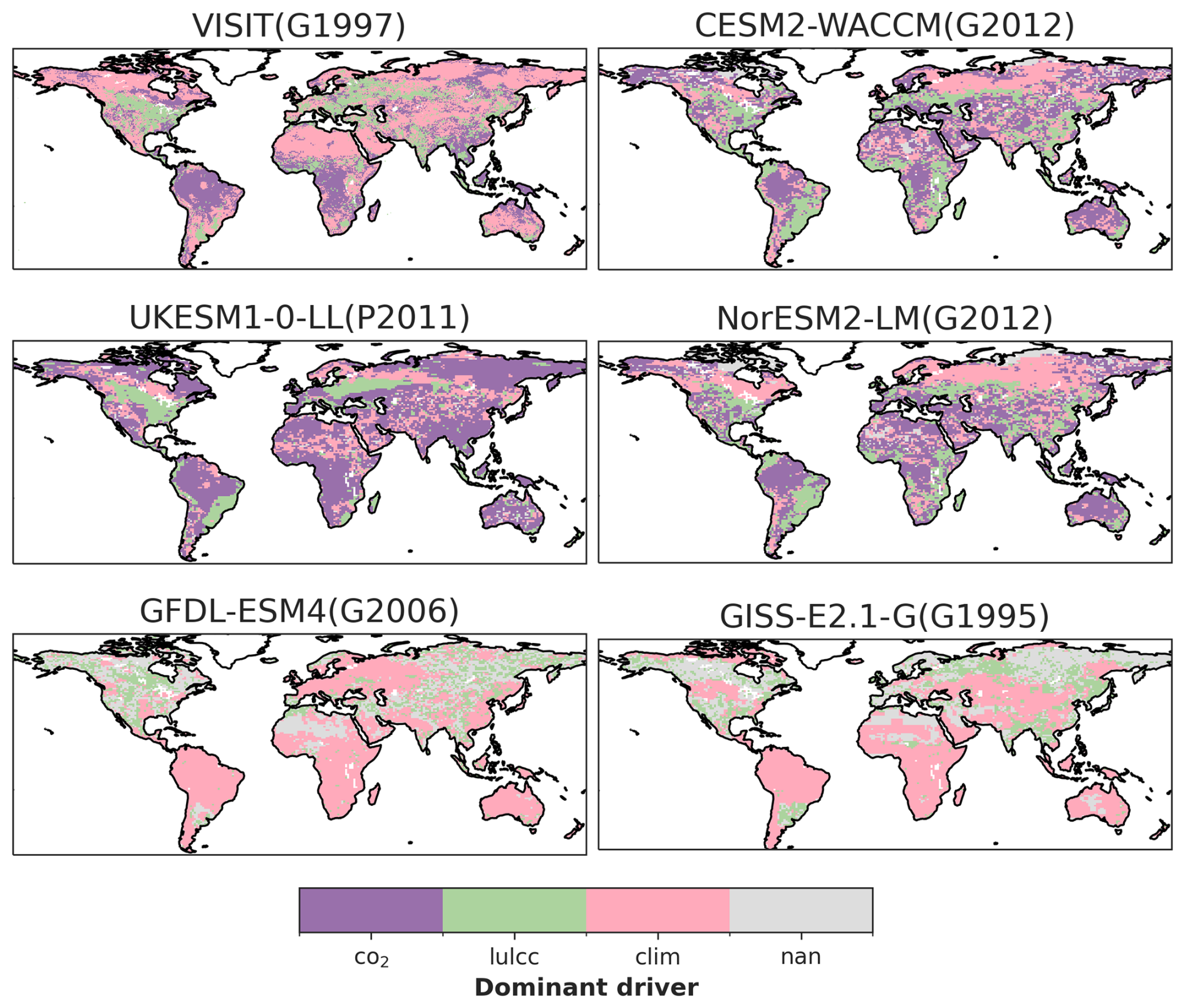
Figure 11 Dominant driver of isoprene emission trends between 1850 and 2014. For each grid, the factor generating the absolute largest trend is selected as the dominant driver. “nan” denotes no significant trend in isoprene emissions because of any factor. It is noteworthy that GFDL-ESM4(G2006) and GISS-E2.1-G(G1995) do not include the CO₂ effects.

Regionally, VISIT(G1997), CESM2-WACCM(G2012), NorESM2-LM(G2012), and UKESM1-0-LL(P2011) identify CO₂ effects as the primary driver of isoprene emissions in tropical regions such as the Amazon and central Africa (Fig. 11). Whereas CO₂ increases emissions in the first three models, it engenders a decrease in UKESM1-0-LL(P2011). LULCC emerges as the dominant driver across all models despite variations in emission schemes and climate factors in Southeast Asia and Europe. West Africa and East Africa show a more complex picture: VISIT(G1997), CESM2-WACCM(G2012), and NorESM2-LM(G2012) identify LULCC in addition to CO₂ as the primary drivers there, while UKESM1-0-LL(P2011) points to CO₂ and GFDL-ESM4(G2006) and GISS-E2.1-G(G1995) point to climate. Southeastern South America also presents discrepancies: CESM-WACCM(G2012), NorESM2-LM(G2012), and UKESM1-0-LL(P2011) indicate LULCC as the main driver, while VISIT(G1997) and the other two models indicate climate factors.

Figure 12 highlights the distinct contributions of individual climate factors to long-term trends in isoprene emissions across models between 1850 and 2014. These differences reflect the varying spatial distributions of the climate variables themselves. Temperature and radiation stand out for their large contributions, while precipitation plays a minor role in most CMIP6 models. Temperature's effects reach a peak in tropical regions, while radiation's influence is greatest in the tropics and some middle and high northern latitudes in these models. VISIT(G1997) stands alone, with both temperature and precipitation exerting stronger effects than radiation. This finding might be attributable to VISIT's big-leaf canopy model, which is less responsive than other models to changes in radiation. The effect of precipitation is particularly pronounced in the tropics, whereas temperature plays a leading role in southeastern South America and East Africa. Unsurprisingly, one key point of agreement across models is that temperature increases generally engender higher isoprene emissions across most regions, reflecting the well-established relation captured by most models. Conversely, surface radiation typically engenders decreases in most models, with VISIT(G1997) again being the exception. Precipitation-driven changes remain highly uncertain, in both magnitude and sign of the trends. For example, VISIT(G1997) shows marked increases in Amazonia emissions because of increased precipitation, whereas UKESM1-0-LL(P2011) projects a decrease in the same region because of reduced precipitation. This discrepancy results from the different climate datasets: VISIT(G1997) relies on reanalysis data, while UKESM1-0-LL(P2011), like other CMIP6 models, uses its own modelled climate data (Fig. S7).

Figure 13 paints a contrasting picture of dominant climate drivers for isoprene emissions across models. Temperature reigns supreme across most regions for models using the Guenther scheme, affecting emission changes in 59 %, 69 %, and 73 % of the global area in GFDL-ESM4(G2006), VISIT(G1997), and GISS-E2.1-G(G1995), respectively. This figure greatly exceeds the 40 %–46 % influence observed for other CMIP6 models. By contrast, UKESM1-0-LL(P2011) stands out, with radiation leading in nearly half of the global land area (45 %), compared to the 24 %–38 % range for other CMIP6 models. VISIT(G1997) stands apart from CMIP6 models by demonstrating a limited effect of radiation on emission changes, affecting only 7 % of the global land area. Precipitation's effects on isoprene emission trends vary markedly among models. GISS-E2-1-G(G1995) and GFDL-ESM4(G2006) show minimal effects, with precipitation dominating only 3.5 % and 8 %, respectively, of global land area. Other models exhibit moderate effects, with precipitation affecting 20 %–25 % of global land area.

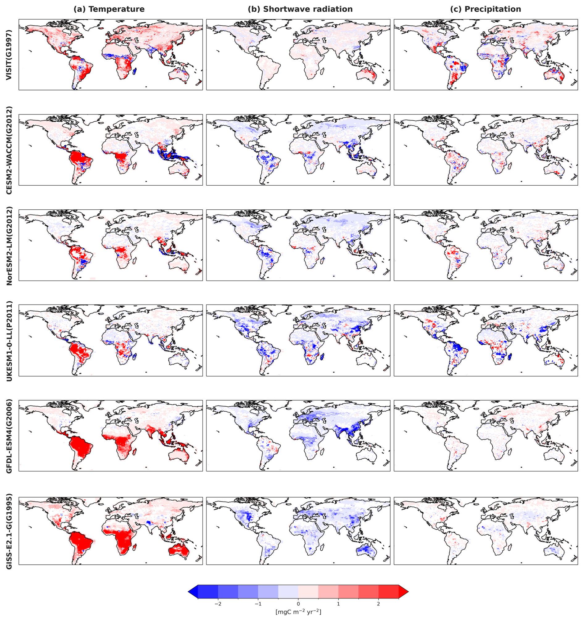
Figure 12 Spatial distribution of the contribution of each climate factor – (a) temperature, (b) shortwave radiation, and (c) precipitation – to the isoprene emission trends in each model. Only significant trends (with p<0.05) are presented.

On a regional scale, the dominant meteorological driver of isoprene emission changes differed substantially among models. In the Amazon, VISIT(G1997) identifies precipitation as the primary driver, whereas the other models point to temperature. Central Africa and Southeast Asia show similar patterns, with temperature dominating in all models except UKESM1-0-LL(P2011), in which radiation and precipitation jointly exert influences. In mid-latitude and high-latitude northern regions, radiation leads across models, although VISIT(G1997) shows a weaker effect. All models show agreement on the considerable influence of precipitation in specific arid and semiarid regions such as the Sahara and South Asia. In Australia, temperature dominates in GFDL-ESM4(G2006) and GISS-E2.1-G(G1995), while VISIT(G1997) identifies precipitation as the dominant factor. However, UKESM1-0-LL(P2011) shows no significant trend in isoprene emissions attributable to any meteorological factor in this region.

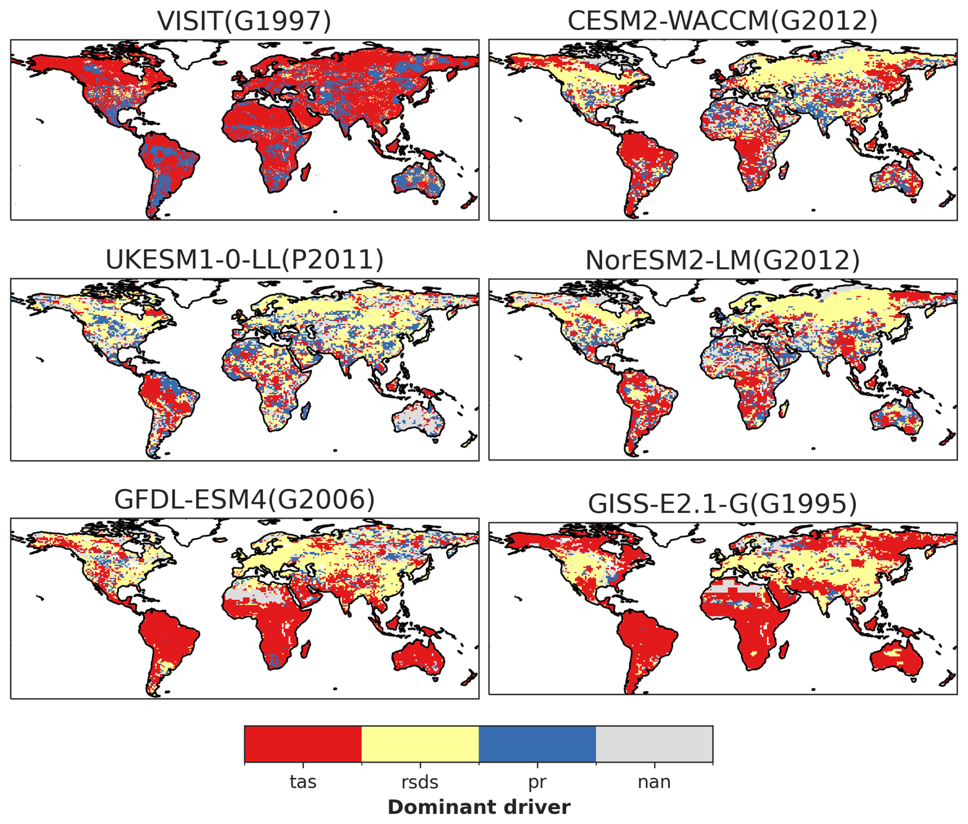
Figure 13 Dominant meteorological drivers of isoprene emission trends during 1850–2014. For each grid, the factor generating the absolute largest trend is selected as the dominant driver. “nan” denotes no significant trend in isoprene emissions attributable to any factor.

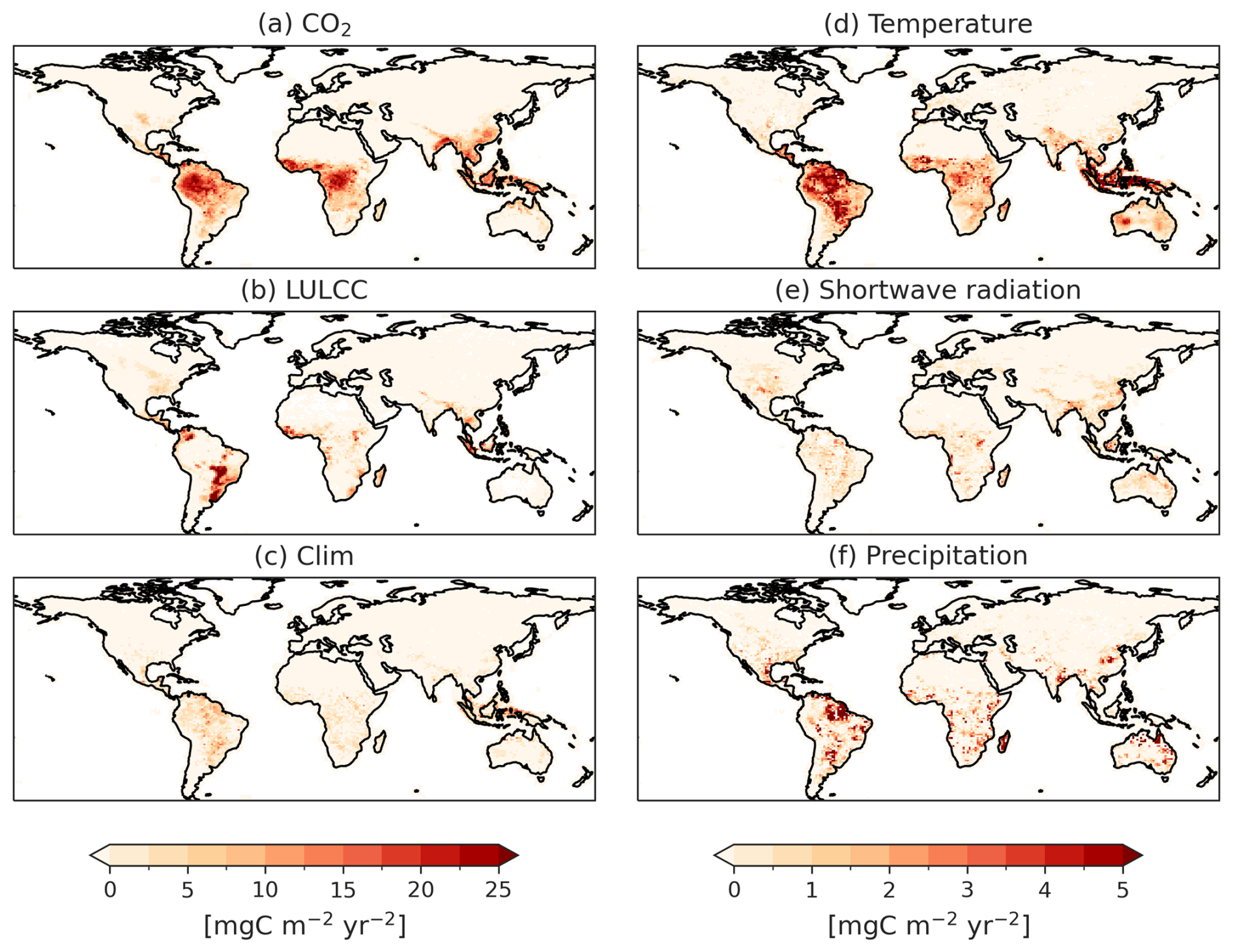
Figure 14 Inter-model spreads of isoprene emission trends attributable to the following: (a) CO₂; (b) LULCC; (c) combined effects of three climate factors; and (d–f) the respective climate factors of temperature, shortwave radiation, and precipitation.

Figure 14 shows the inter-model spread, representing the standard deviation of isoprene emission trends attributable to each factor, calculated for each grid cell across all models. The inter-model spreads of isoprene emission trends are located primarily in tropical areas and the Southern Hemisphere (Fig. 14). The highest uncertainty in the contribution of CO₂ to isoprene emission trends in tropical areas (Fig. 14a) arises from inconsistencies in CO₂ effects among models. CO₂ consistently shows a positive influence on isoprene emissions in the tropics in VISIT(G1997), CESM2-WACCM(G2012), and NorESM2-LM(G2012), but it has a negative effect in UKESM1-0-LL(P2011) (Fig. 10a). Also, uncertainties in LULCC effects on isoprene trends are most concentrated in southeastern South America and Southeast Asia (Fig. 14b). The reason underlying uncertainties in LULCC effects might arise from variations in original land cover maps, land use schemes, and emission factors across models. For instance, in southeastern South America, CESM2-WACCM(G2012) and UKESM1-0-LL(P2011) simulate a stronger effect of LULCC because of that region's conversion of forest to cropland compared to GFDL-ESM4(G2006), which shows more minor changes in isoprene emissions, mainly because of its conversion of grassland to cropland, as shown in Fig. S4. In contrast, inter-model differences driven by climate factors are more minor than those for CO₂ and LULCC (Fig. 14c). This is true because the inhomogeneous effects of different climate elements on isoprene emissions tend to offset each other to a large degree (Figs. 10c and 12). Among the climate variables, uncertainties in the effects of temperature on isoprene trends are concentrated in the tropics, whereas those for radiation are concentrated in middle northern latitudes (e.g. central North America and East Asia) and those for precipitation in parts of the Amazon, Madagascar, and northern Australia.

4 Discussion and perspective

4.1 Sources of uncertainty

4.1.1 Variability in regional isoprene emissions

Models show remarkable consistency in estimation of the global quantities of isoprene emissions for recent times, but considerable regional discrepancies exist (Fig. 1b). Tropical regions, notably the Amazon (98–175 TgC yr⁻¹) and Southeast Asia (14.7–87.8 TgC yr⁻¹), exhibit the greatest variability. Arid regions such as the Sahara also displayed wide ranges (0.1–24.9 TgC yr⁻¹) (Table S4). The main reason underlying these regional discrepancies appears to be differences in how models represent plant functional types (PFTs) and emission factors assigned to each PFT across the models (Tables S6 and S7). For instance, the latest Guenther scheme (G2012) used in CESM2-WACCM(G2012) and NorESM2-LM(G2012) incorporated 16 PFTs, compared to 7 or 11 PFTs in the older versions used by GFDL-ESM4(G2006) or GISS-E2.1-G(G1995) and 16 PFTs for VISIT(G1997). For the P2011 scheme, 13 PFTs were used for UKESM1-0-LL(P2011). Moreover, the definitions of these PFTs vary among models, influencing their emission factors (Table S7). For instance, in the G2012 scheme, emission factors for broadleaf trees (evergreen vs. deciduous) across tropical, temperate, and boreal regions range from 20.6 to 52.4 µgC g${}_{\mathrm{mass}}^{-\mathrm{1}}$ h⁻¹, with the highest emissions from broadleaf deciduous boreal trees. Also, VISIT(G1997) assigned emission factors of 8–45 µgC g${}_{\mathrm{mass}}^{-\mathrm{1}}$ h⁻¹ to five broadleaf trees, but the highest emission factor was assigned to broadleaf deciduous temperate trees. The emission factor for a single broadleaf tree type in the G2006 scheme is only 24 µgC g${}_{\mathrm{mass}}^{-\mathrm{1}}$ h⁻¹, whereas the G1995 scheme assigns 24 µgC g${}_{\mathrm{mass}}^{-\mathrm{1}}$ h⁻¹ for broadleaf evergreen trees and 24/45 µgC g${}_{\mathrm{mass}}^{-\mathrm{1}}$ h⁻¹ for two broadleaf deciduous trees depending on whether they are cold- or drought-tolerant. The P2011 scheme uses emission factors ranging from 16–35 µgC g${}_{\mathrm{mass}}^{-\mathrm{1}}$ h⁻¹ assigned for three broadleaf tree types, with the highest emission for broadleaf deciduous trees across all regions.

These variations in PFT representation and emission factors strongly influence the spatial distributions of isoprene emissions among models. For instance, in the Amazon, G2012 assigned a tree fraction of roughly 74 ± 0.13 % between 2000 and 2014, while G2006 and G1995 allocated only 34 ± 0.23 %. By contrast, G2006 estimated a larger grass fraction (36 ± 2.50 %) compared to G2012 (21 ± 0.14 %) (Fig. S4). Although these models did not provide specific information related to tree types, broadleaf evergreen trees are generally predominant in this region, emitting more isoprene than grasses (Table S7). This greater emission explains why the higher tree fraction of G2012 caused markedly higher total isoprene emissions for the Amazon (175 TgC yr⁻¹) than the average isoprene emissions in G2006 and G1995 (103 TgC yr⁻¹). Also, VISIT(G1997) and P2011, with similar emission factors for broadleaf evergreen trees and C₄ grass (24 µgC g${}_{\mathrm{mass}}^{-\mathrm{1}}$ h⁻¹), exhibited comparable emissions in this region (133 vs. 117 TgC yr⁻¹). P2011 allocated a tree fraction of approximately 75 ± 0.20 %, similar to that of G2012, and a grass fraction of 11.7 ± 0.13 %, half that of G2012. The emission factor for broadleaf evergreen trees in G2012 (20.6 µgC g${}_{\mathrm{mass}}^{-\mathrm{1}}$ h⁻¹) is slightly lower than that in P2011 (24 µgC g${}_{\mathrm{mass}}^{-\mathrm{1}}$ h⁻¹), but the emission factor for C₄ grass in P2011 (24 µgC g${}_{\mathrm{mass}}^{-\mathrm{1}}$ h⁻¹) is notably 20 times higher than in G2012 (1.2 µgC g${}_{\mathrm{mass}}^{-\mathrm{1}}$ h⁻¹), which was identified as a bug in P2011 (Weber et al., 2023) and which was corrected in current development strands of UKESM1-0-LL. However, compensation effects between the two plant types cannot fully explain the lower isoprene emissions in UKESM1-0-LL(P2011) than CESM2-WACCM(G2012) over the Amazon. Another reason might be the difference in the isoprene emission scheme between these models, such as the scaling factor to adjust for variations in standard temperature (297 K in the Guenther scheme vs. 303.15 K in P2011) for setting basal emission factors. This hypothesis, suggesting that emission factors strongly influence the spatial distribution of isoprene emissions and regional quantities of isoprene emissions, is further supported by reductions observed when using different emission factors in VISIT(G1997) (Ito, 2019b). Applying the standard high emission factor (24 µgC g${}_{\mathrm{mass}}^{-\mathrm{1}}$ h⁻¹) yielded global isoprene emissions of 510 TgC yr⁻¹, while the lower emission factor (9 µC µgC g${}_{\mathrm{mass}}^{-\mathrm{1}}$ h⁻¹), based on Malaysian observations for broadleaf evergreen forests (Saito et al., 2008), reduced mean global emissions to 342 TgC yr⁻¹ (33 %) during 2000–2014, with Amazonia emissions dropping from 133 to 62 TgC yr⁻¹ (54 %). Similarly, the stronger isoprene emissions simulated by the GISS-E2.1-G(G1995) in northern Australia and the Sahara likely arise from a higher proportion of shrubs with higher emission factors in its vegetation representation compared to other models, which grasses might dominate (Figs. S4 and S8). However, changes in PFTs and their associated emission factors primarily influence the spatial distribution of isoprene emission, not the seasonality, in VISIT(G1997) and other models employing MEGAN or P2011 schemes (Henrot et al., 2017; Weber et al., 2023). Unfortunately, assessing details of the uncertainty arising from PFTs and their differences in emission factors is beyond the scope of this study because of the lack of necessary output data available from the CMIP6 models. However, future efforts to establish a standardized global PFT map with corresponding PFT-specific emission factors hold great promise for reducing these uncertainties and for improving the consistency of simulations across different models.

Current approaches that use generalized PFT emission factors may oversimplify the effects of climate-driven shifts in vegetation composition. Changes in tree species distribution and composition in response to climate change affect the quantity and composition of BVOC emissions. Isoprene emission rates vary widely across plant species, and assigning emission factors to specific PFTs is often not unambiguous. Plant-specific emission factors would more accurately represent the impacts of individual climate drivers, as emission factors can differ greatly even within the same genus (Karl et al., 2009; Satake et al., 2024). Dani et al. (2014) suggested that the trait of isoprenoid emission in evergreen plants can be lost during evolution in favour of more storable compounds (monoterpenes) to better cope with repeated and prolonged stress. Additionally, the proportion of isoprene-emitting tropical trees appears to increase with mean annual temperature but decrease with the length of the dry season (Taylor et al., 2018). These findings suggest that future model developments should also consider plant-specific emission factors and phenological changes to accurately assess the impacts of climate-driven changes in tree species distribution and composition on BVOC emissions.

4.1.2 Variability in attribution to isoprene emissions

In recent decades (1980–2014), all the models detected an overall increasing trend in global isoprene emissions, which agrees with findings from earlier studies using satellite data with MEGAN (Opacka et al., 2021). However, the main drivers of this trend differed among the models (VISIT and the CMIP6 models) (Fig. 6) depending on the assumptions considered in the parameterization (Table S1). These models agree that the CO₂ fertilization effect is dominant over the CO₂ inhibition effect in MEGAN-based models for this period. Alternatively, there are compensatory effects between CO₂ inhibition and temperature in P2011 (Pacifico et al., 2012). This finding in MEGAN-based models in our study aligns with those findings reported by Heald et al. (2009), who claimed that while CO₂ inhibition partially offsets the effect of rising temperatures on isoprene emissions, it does not fully compensate for the total effects of rising temperature and vegetation productivity. This inadequate compensation underscores the important role of CO₂ fertilization in future isoprene emission changes, as well as in trends observed for recent decades (1980–2014) in our study, which are partially reflected in the future snapshot simulation (2100) in the earlier study (Heald et al., 2009). Further investigation into isoprene emission trends and their controlling factors in future simulations (2015–2100) under CMIP6 ScenarioMIP (SSP) is necessary to validate the robustness of these findings. The magnitude of the net CO₂ effect remains highly uncertain, depending on the model scheme and how it accounts for CO₂ inhibition, if at all. Additionally, LULCC had a moderate effect on the emission trends in these models. By contrast, models without CO₂ effects (GFDL-ESM4(G2006) and GISS-E2.1-G(G1995)) showed a minimal influence of LULCC on the emission trends, whereas climate effects dominated, leading to lower increasing trends compared to other MEGAN-based models.

Regarding long-term trends (1850–2014), CESM2-WACCM(G2012) and NorESM2-LM(G2012) showed minimal changes in isoprene emissions (Figs. 6 and 7) because the CO₂ effects balanced out the LULCC effects. VISIT(G1997) exhibited trends that were more positive than those of either CESM2-WACCM(G2012) or NorESM2-LM(G2012) because of its inclusion of CO₂ fertilization but exclusion of CO₂ inhibition. Even with CO₂ inhibition included, CESM2-WACCM(G2012) and NorESM2-LM(G2012) showed long-term trends for isoprene emissions driven by CO₂ similar to those of VISIT(G1997) (Fig. 6). This similarity of trends suggests that CO₂ fertilization predominates over CO₂ inhibition, which might only become active when CO₂ concentrations exceed a threshold (e.g. 365 ppm in these models). The average isoprene emissions attributed to CO₂ in CESM2-WACCM(G2012) and NorESM2-LM(G2012) during 2000–2014 (1.259 TgC yr⁻²) were lower than the average in VISIT(G1997) (1.714 TgC yr⁻²). UKESM1-0-LL(P2011) exhibited a significant and negative trend in isoprene emissions because of the combined effects of CO₂ and LULCC. This singularity of UKESM1-0-LL(P2011) might be attributable to its different isoprene emission scheme (P2011), particularly its methodology to treat CO₂ effects (direct inhibition and indirect fertilization via photosynthesis (GPP) parameterization) compared to MEGAN-based models. Despite radiation-induced decreases, GFDL-ESM4(G2006) and GISS-E2.1-G(G1995) displayed increasing trends driven by rising temperatures. Among the three drivers (CO₂, LULCC, and climate), the CO₂ effects on isoprene emissions have the highest inter-model variability (σ=0.43 TgC yr⁻²), followed by LULCC (σ=0.17 TgC yr⁻²) and climate change (σ=0.06 TgC yr⁻²). Therefore, the different mechanisms used for the respective models to account for CO₂, LULCC, and climate effects contribute to the uncertainty in long-term global isoprene emission trends. Particularly addressing CO₂ and LULCC effects, rather than meteorological factors alone, is crucially important for the use of long-term models. All the models show agreement in terms of a significant increase from 1980 to the present, but pre-1980 trends remain uncertain, highlighting the need for improved historical data and refined model evaluation to capture past trends better and to enhance the accuracy of future predictions.

Regarding spatial distribution, the models without CO₂ effects (GFDL-ESM4(G2006) and GISS-E2.1-G(G1995)) generally predict a weaker gradient in isoprene emissions compared to other models (Fig. 5). This difference likely arises because isoprene emissions are not tied interactively to vegetation production in these two models. Higher CO₂ can either directly reduce (inhibition) or indirectly increase isoprene emissions because of enhanced vegetation production (represented by LAI in MEGAN or GPP in P2011). It is true that CESM2-WACCM(G2012), NorESM2-LM(G2012), UKESM1-0-LL(P2011), and VISIT(G1997) captured the indirect CO₂ effects, but VISIT(G1997) neglected the direct inhibition effect. Nevertheless, both effects were considered in CESM2-WACCM(G2012), NorESM2-LM(G2012), and UKESM1-0-LL(P2011). As the dominant driver in tropical regions (Fig. 11), CO₂ effects strongly influence the global isoprene emission trends. These regions are high emitters because of sustained warm temperatures, intense radiation, and high biomass density, coupled with high emission factors of tropical vegetation types (Henrot et al., 2017). The inter-model spread of CO₂'s contribution to isoprene emission trends is particularly pronounced in tropical areas, surpassing the spread associated with LULCC and climate effects (Fig. 14). This suggests that further model refinement is needed, particularly in accurately representing CO₂ effects on isoprene emissions in tropical regions.

Compared to temperature and radiation, precipitation is found to play a minor role in controlling long-term trends of isoprene emissions in most CMIP6 models. However, the effect of extreme climate events, such as drought stress, on isoprene emissions is uncertain because of limitations in the algorithms representing drought impacts. While UKESM1-0-LL(P2011) and VISIT(G1997) account for indirect drought effects through photosynthesis, only NorESM2-LM(G2012) models direct effects using its own soil moisture data and MEGANv2.1-based wilting points (Chen and Dudhia, 2001). These default wilting points are likely too low, failing to capture drought impacts like those of 2011 and 2012 (Jiang et al., 2018; Sindelarova et al., 2014). Besides wilting point selection, soil moisture inputs, which are challenging to simulate globally, further affect the performance of drought stress algorithms (Opacka et al., 2022; Potosnak et al., 2014b; Wang et al., 2022). Jiang et al. (2018) developed the MEGAN3 approach of using a photosynthesis parameter and a soil wetness factor to determine the drought activity factor, which improves the simulation of isoprene emissions in non-drought and drought periods at the Missouri Ozarks AmeriFlux (MOFLUX) field site. Klovenski et al. (2022) found that emulating MEGAN3's drought stress representation in GISS-ModelE, a current development strand of GISS-E2.1-G, requires model-specific tuning and that applying drought stress factors can improve simulations for models that overestimate isoprene emissions. Other drought indicators (e.g. the ratio of actual evapotranspiration to potential evapotranspiration) may be more effective than soil moisture in capturing drought impacts (Wang et al., 2022). These global simulations underpin the importance of accurately simulating the drought-induced response of isoprene emission in ESMs, as well as the need to expand studies beyond MOFLUX to diverse ecosystems to validate and refine drought stress algorithms for ESMs.

4.1.3 Uncertainty in modelling CO₂ effects on isoprene emissions

Changes in atmospheric CO₂ levels are expected to greatly alter biogenic isoprene emissions. With CO₂ levels predicted to be doubled under the SSP3-7.0 scenario (and even higher increases under SSP5-8.5 or smaller increases under SSP2-4.5 and SSP1-2.6) by the end of this century, producing accurate models of the CO₂ effects on isoprene emissions is fundamentally important. In fact, CO₂ effects, including the fertilization effect, increase vegetation productivity (LAI/GPP), which is a key driver of photosynthesis and isoprene emission. However, considerable inter-model differences were found for simulation of this effect within the C4MIP project (Friedlingstein et al., 2006; Hajima et al., 2014; Arora et al., 2020). Models overestimating the LAI/GPP response to rising CO₂ are likely to overestimate CO₂ fertilization effects on ecosystem productivity and ensuing isoprene emission uncertainties. Direct CO₂ inhibition effects also lack clear consensus among models. Understanding the physiological response of isoprene emissions to the combined effects of rising CO₂ and temperature is vital for projecting future emissions under climate change. However, the mechanisms controlling isoprene emissions remain uncertain, yielding conflicting hypotheses. Some results of studies suggest that future high CO₂ levels might suppress isoprene emission, potentially counteracting the stimulating effects of rising temperatures or the combined effects of temperature increase and enhanced vegetation productivity, which might result in minimal change compared to the present day (Arneth et al., 2007b; Pacifico et al., 2012), an overall increase (Heald et al., 2009), or even a decrease in global isoprene emissions (Hantson et al., 2017). Alternatively, others propose that CO₂ inhibition might become less effective at high temperatures (above 30 °C) (Lantz et al., 2019; Monson et al., 2016; Potosnak et al., 2014a; Sun et al., 2013), potentially leading to a net increase in emissions driven by temperature (Lantz et al., 2019; Potosnak et al., 2014a). In contrast, some studies imply stable emission under preindustrial conditions with lower CO₂ levels (Heald et al., 2009); others suggest higher emissions than those of recent times (Arneth et al., 2007a; Hantson et al., 2017; Lathière et al., 2010; Pacifico et al., 2012; Unger, 2013). Both sets of modelling studies entail uncertainties; yet, in the absence of measurements or proxies, modelling serves as our sole resort for estimating preindustrial isoprene emission rates.

From preindustrial times to the present day, some models have exhibited a decline in isoprene caused by strong CO₂ inhibition (Arneth et al., 2007a; Lathière et al., 2010; Pacifico et al., 2012), similarly to UKESM1-0-LL(P2011) in this study. Others imply no trend with weak inhibition (Heald et al., 2009), similarly to CESM2-WACCM(G2012) and NorESM2-LM(G2012) in this study. However, CMIP6 and VISIT-S3(G1997) show consistency in key climate variables (temperature, radiation, and precipitation) on a global anomaly basis (Fig. S5). These models share the same photosynthesis schemes, explaining the identical upward trends found for GPP/LAI represented for the CO₂ fertilization effect (Fig. S6). Therefore, the discrepancy in CO₂-driven isoprene emission trends likely derives from differences in the implemented CO₂ inhibition schemes.

Both the MEGAN and P2011 models base their CO₂ inhibition scheme on the same observational experiment of two mild temperate vascular plants (Possell et al., 2005). However, as presented in Fig. 1 of Heald et al. (2009) and Fig. 8 of Arneth et al. (2007b), the two models diverge considerably in their response curves. Specifically, the MEGAN-based scheme would only reduce isoprene emissions for CO₂ levels above 365 ppm and at a lower rate than the P2011-based scheme. Both models normalize emission rates based on the values for the year 2000 (Arneth et al., 2007b; Heald et al., 2009; Possell et al., 2005), but there is a difference in the CO₂ inhibition factor for the preindustrial period.

At 280 ppm of CO₂ (preindustrial level), the MEGAN-based scheme maintains a CO₂ inhibition factor of around 1, whereas the P2011-based scheme gives a CO₂ inhibition factor of approximately 1.5 (Arneth et al., 2007b). This higher value found for the latter implies a 30 % increase in isoprene emissions efficiency in the preindustrial period and a subsequent decrease to present-day levels. In fact, this difference likely explains the divergent long-term emission trends presented in Fig. 4.

Additional uncertainty arises at lower CO₂ concentrations (e.g. 185 ppm of the Last Glacial Maximum), for which MEGAN implies stability (Heald et al., 2009) and P2011 estimates much higher emissions than those of the present day (Hopcroft et al., 2017; Pacifico et al., 2012). This discrepancy might add further uncertainty to the interpretation of trends and their influence on atmospheric composition (i.e. methane lifetime) in past atmospheres (Achakulwisut et al., 2015; Hopcroft et al., 2017). Although several studies have consistently demonstrated that elevated CO₂ levels inhibit isoprene emissions (Feng et al., 2019; Niinemets et al., 2021; Possell et al., 2005; Possell and Hewitt, 2011), only one study has demonstrated a marked increase at low CO₂ levels (185 ppm) (Possell et al., 2005). Further research is necessary to refine CO₂ inhibition–enhancement parameterizations and to enhance our understanding of this complex relation at low CO₂ levels. Additionally, some results of short-term field studies show that high temperatures might weaken CO₂ inhibition, necessitating its integration into models for accurate future predictions (Lantz et al., 2019).

Furthermore, a recent study (Niinemets et al., 2021) has highlighted the diversity in plant responses to CO₂-induced isoprene emission changes. Some species such as poplar (common in temperate and boreal regions) are apparently more sensitive than others, such as oak and mango (found in temperate to tropical regions). The variation in plant CO₂ responsiveness can be attributed to differences in substrate availability, implying that using a single CO₂ inhibition function and threshold for all plants in emission models might overestimate or underestimate this effect. Additionally, the existing scheme relies primarily on temperate species, raising concerns about its accuracy for tropical species (Pacifico et al., 2012; Young et al., 2009). Because tropical plants are the major contributors to global isoprene emissions, better understanding of their long-term response to CO₂ is valuable. Developing diverse CO₂ inhibition functions for different species, especially those in tropical regions, is necessary for accurate prediction of the effects of rising CO₂ on future isoprene emissions and, in turn, their effects on Earth's atmosphere and ecosystems.

4.2 Suggestions for future development

As explained above, the reliance on single-function CO₂ inhibition schemes for all plant species hinders accurate predictions. Future models must incorporate diverse PFT-specific inhibition functions, particularly for tropical species, which dominate global isoprene emissions. Furthermore, long-term studies across ecosystems must be conducted to confirm the weakening effects of high temperatures on CO₂ inhibition for a diversity of plant species. Then this effect must be integrated into current models. Accurate representation of LAI and GPP in land models is extremely useful for simulating the effects of CO₂ fertilization on isoprene emissions. Validation against high-resolution satellite imagery, especially in tropical regions with complex vegetation cover, is necessary for this purpose. Current uncertainties related to LULCC effects might also arise from the employment of constant emission factors for PFTs. For instance, deforestation might decrease emissions by replacing high-emitting broadleaf trees with crops, but oil palm, a higher emitter than broadleaf trees, can increase emissions in some cases (e.g. Malaysia) (Misztal et al., 2011; Opacka et al., 2021; Stavrakou et al., 2014; Tanaka et al., 2012). Additionally, neglecting grass and shrub fractions beyond tree cover can contribute further to LULCC effect uncertainty.

Even though random forest regression can replicate global isoprene emissions from all CMIP6 models (Fig. S2), we advocate for the additional multi-model intercomparison of land system models under the TRENDY project's GPP estimation protocols (Friedlingstein et al., 2022; Sitch et al., 2015, 2024), applying similar settings to isoprene emissions. Such multi-model intercomparison will help to pinpoint the important contributors to uncertainty in isoprene emission estimates. Furthermore, leveraging and expanding the existing FLUXNET network (Baldocchi et al., 2001; FLUXNET Portal, 2024) ground-based isoprene emissions observation can provide valuable data for validating long-term isoprene emission models across various regions. We can also develop independent data-driven estimates using machine-learning methods based on these long-term data. These estimates can enhance our understanding of historical isoprene emission changes and can improve the reliability of future predictions.

Current ESMs, including the latest CMIP6 experiments, rely primarily on only two schemes for estimating past, present, and future isoprene emissions: photosynthesis-based models (e.g. P2011) and empirically based models (e.g. MEGAN). These approaches offer some benefits, but they entail some limitations. The photosynthesis-based models estimate isoprene emissions based on photosynthetic electron transport products, capturing light dependence. However, evidence suggests this might not accurately reflect long-term responses to temperature and CO₂ changes that are invaluable for decadal and millennial emission projections (Sharkey and Monson, 2014). Additionally, these models do not account for potential substrate effects under future climate conditions, which can strongly influence CO₂ and temperature dependence of isoprene emissions. The empirical model estimates isoprene emissions based on two factors: the temperature dependence of enzyme–substrate interactions and empirical data of emission reductions observed for plants grown under different atmospheric CO₂ concentrations. However, the adjustments to some driving parameters in MEGAN lack a clear mechanistic connection to underlying biochemical processes (Monson et al., 2007; Sharkey and Monson, 2014). The reliance on these two schemes with their inadequate representation of biochemical processes, can engender inaccuracies and uncertainties in predicting long-term isoprene emissions under varying environmental conditions. To overcome this limitation, more intensive and comprehensive studies must be conducted to develop a broader range of isoprene and other BVOC emission schemes that better capture the complexity and diversity of biogenic emissions. By incorporating a broader array of emission models, researchers can augment the accuracy and reliability of BVOC emission predictions, especially in the context of evolving environmental conditions and climate scenarios. This diversity in BVOC emission schemes is extremely valuable for advancing our understanding of biogenic emissions and their effects on atmospheric chemistry and climate dynamics. Moreover, this diversity underscores the necessity for additional research to refine the representation of BVOC emissions in ESMs.

5 Conclusions

This study comprehensively analysed trends in isoprene emissions and their controlling factors during 1850–2014 using long-term isoprene emissions datasets derived from offline simulations of the VISIT dynamic global vegetation model and online estimates from CMIP6 ESMs. The models, except for UKESM1-0-LL(P2011), incorporate empirical schemes such as MEGAN, categorized into four groups based on their isoprene emission schemes: (1) MEGAN with CO₂ fertilization only, which is VISIT(G1997); (2) MEGAN with CO₂ effects (fertilization and inhibition), which comprise CESM2-WACCM(G2012) and NorESM2-LM(G2012); (3) MEGAN without CO₂ effects, which comprise GFDL-ESM4(G2006) and GISS-E2.1-G(G1995); and (4) photosynthesis-based with CO₂ effects, which is UKESM1-0-LL(P2011).

In the present day (2000–2014), mean global isoprene emissions estimated from all models are consistent, with an inter-model spread of only 24 TgC yr⁻¹ (5 %), ranging from 434 to 510 TgC yr⁻¹. However, regional emissions vary considerably, with an inter-model spread ranging between 0.53 and 30.77 TgC yr⁻¹ (9 %–212 %), primarily because of differences in PFT composition and emission factors. Standardizing global PFT maps with specific emission factors can reduce these uncertainties and can improve simulation consistency across models.

Over the historical period examined for this study (1850–2014), isoprene emission trends vary widely across models. Empirical models without CO₂ effects (GFDL-ESM4(G2006) and GISS-E2.1-G(G1995)) show slightly increasing trends, whereas the model considering only the CO₂ fertilization effect, VISIT-S3(G1997), estimates a significant increasing trend. Models including both CO₂ effects (fertilization and inhibition) show no change (CESM2-WACCM(G2012) and NorESM2-LM(G2012)). The sole photosynthesis-based model, UKESM1-0-LL(P2011), exhibits a sharply decreasing trend. These variations in global long-term trends are attributable to differences in the main drivers among models. Similarly to VISIT(G1997) with only CO₂ fertilization, MEGAN-based models with CO₂ effects (CESM2-WACCM(G2012) and NorESM2-LM(G2012)) emphasize CO₂ fertilization, potentially underestimating CO₂ inhibition. Also, UKESM1-0-LL(P2011) suggests that CO₂ inhibition outweighs fertilization, possibly because of its distinct representation of CO₂ inhibition. MEGAN-based models without CO₂ effects (GFDL-ESM4(G2006) and GISS-E2.1-G(G1995)) attribute the trend primarily to climate factors, chiefly rising temperatures.

Globally, models vary widely in their estimates of CO₂ effects on isoprene emissions, in both direction and magnitude, alongside moderate differences in LULCC-induced emission reductions and relative consensus on climate-driven emission increases. Divergence in CO₂-driven emission trends likely stems from models' different CO₂ inhibition representations, which can counteract increasing isoprene emission trends attributable to rising temperatures or in combination with CO₂ fertilization. At the grid cell level, the highest inter-model variability in simulated isoprene emission trends occurs in regions such as the Amazon, Southeast Asia, and southeastern South America, influenced primarily by CO₂ and LULCC.

The discrepancies among models highlight the importance of studying isoprene emission trends and the caution which is necessary for interpreting plant–climate interactions using long-term isoprene emission estimates. Results of our study emphasize the need for deeper investigation of CO₂ and LULCC effects on isoprene emissions because their influence on long-term trends far surpasses short-term variations induced by climate factors. Expanding long-term observation networks and refining models by considering diverse species-specific responses to changing CO₂ levels in different ecosystems are necessary. Current-generation ESMs rely on empirical and photosynthesis-based approaches to estimate isoprene emissions, each with their idiosyncratic benefits and limitations. Developing more comprehensive emission schemes that better reflect the complexity of plant emissions would support more accurate and reliable predictions of how these emissions can be expected to change under different climate conditions, which is necessary for understanding plant–climate interactions via emissions.