Inclusion of the ECMWF ecRad radiation scheme (v1.5.0) in the MAR (v3.14), regional evaluation for Belgium, and assessment of surface shortwave spectral fluxes at Uccle

The MAR (Modèle Atmosphérique Régional) is a regional climate model used for weather forecasting and climate studies over several continents, including polar regions. To simulate how solar radiation and Earth's infrared radiation propagate through the atmosphere and drive climate, MAR uses the Morcrette radiation scheme. Last updated in the 2000s, this scheme is no longer maintained and lacks the flexibility to add new capabilities, such as computing high-resolution spectral fluxes.

This paper presents version 3.14 of MAR, an update that allows MAR to run with ecRad, the latest radiation scheme provided by the European Centre for Medium-Range Weather Forecasts (ECMWF). Operational in the ECMWF's Integrated Forecasting System (IFS) since 2017, ecRad was designed with modularity in mind and is still in active development.

We evaluate the updated MAR by comparing its outputs over 2011–2020 for Belgium to gridded data provided by the Royal Meteorological Institute of Belgium (RMIB) and by the EUMETSAT Satellite Application Facility on Land Surface Analysis. Several sensitivity experiments have been carried out to find the configuration achieving the most balanced radiative budget, as well as to demonstrate that the updated MAR is better equipped to achieve such a balance. Moreover, a MAR simulation running ecRad with high-resolution ecCKD gas-optics models has been conducted to produce spectral shortwave fluxes, which are compared to ground-based spectral measurements captured by the Royal Belgian Institute for Space Aeronomy at Uccle (Belgium; 50.797° N, 4.357° E) in the 280–500 nm range from 2017 to 2020. Finally, as a first application of spectral shortwave fluxes computed by MAR running with ecRad, a method for predicting UV indices is described and evaluated.

1 Introduction

The MAR is a regional atmospheric model that was initially designed by Gallée and Schayes (1994) to study the climate of various regions at high resolution (typically ranging from 5 to 25 km) over periods of time covering a few years up to several decades (Fettweis et al., 2013b). Throughout its decades of development, MAR has been tuned for polar areas in particular, notably by coupling it with a snow model (De Ridder and Gallée, 1998; Gallée et al., 2001). This development allowed MAR users to study the surface mass balance of the Greenland ice sheet starting from the early 2000s (Gallée and Duynkerke, 1997; Lefebre et al., 2003, 2005). Since then, MAR has been run to estimate the future impact of the Greenland ice sheet on sea level rise (Fettweis et al., 2013a) and to predict the evolution of its surface temperatures (Delhasse et al., 2020; Hanna et al., 2020). MAR is also used to study the Antarctic ice sheet (Amory et al., 2021; Kittel, 2021) as well as the evolution of the precipitation regime of various regions, such as western and equatorial Africa (Gallée et al., 2004; Doutreloup, 2019) and central Europe (Wyard et al., 2020; Ménégoz et al., 2020).

A key component of the MAR is its radiative transfer scheme, or radiation scheme. This module simulates how both shortwave (solar) radiation and longwave (Earth's infrared) radiation propagate through the atmosphere and over the surface. To accurately simulate the transfer of radiative energy, a radiation scheme must take into account all optically active components within the atmosphere that either reflect or absorb and scatter radiation (if not both), such as the Earth's surface (and its albedo), greenhouse gases, aerosols, and clouds. Having an accurate radiation scheme is crucial for a climate model, as how the radiative energy flows within the atmosphere and over the surface is what regulates the Earth’s surface temperature. MAR up to version 3.13 uses the Morcrette (1991, 2002) radiation scheme, consisting of two separate schemes for shortwave (solar) radiation and longwave (Earth's infrared) radiation. This scheme was notably used in the ERA-40 reanalysis (Uppala et al., 2005) and is still used in several regional climate models (Jacob et al., 2012; Hourdin et al., 2013).

Developed until the early 2000s, the Morcrette scheme is no longer maintained. Moreover, it has become difficult to update to improve or expand its capabilities due to the lack of modularity of its source code, partly because it pre-dates Fortran 2003, which improved derived types and introduced object-oriented programming in the language (Reid, 2007). The difficulty of updating the Morcrette scheme hinders potential improvements for the MAR, such as producing spectral shortwave fluxes to simulate snow albedo more accurately. Updating the radiation component of MAR also constitutes an opportunity to fix its known radiative biases: MAR running with Morcrette is known for overestimating downward shortwave radiation and underestimating downward longwave radiation, as evidenced by Fettweis et al. (2017), Delhasse et al. (2020), Wyard et al. (2018), and Kittel et al. (2022). Up to version 3.13 (Fettweis et al., 2023), MAR partially mitigates this issue by tuning the outputs of the Morcrette scheme to slightly compensate for known heat flux biases, depending on the simulated region, allowing MAR to simulate a correct near-surface temperature.

This paper discusses the inclusion in the MAR of a new radiative transfer scheme: the ecRad radiation scheme (Hogan and Bozzo, 2018), the latest radiative transfer scheme developed by the ECMWF. Since 2017, ecRad has been used as the radiative transfer component of the operational weather forecast model of the ECMWF, the IFS. The key feature of ecRad is its modularity: its architecture allows users to change independently, among others, the description of optical properties with respect to clouds, greenhouse gases, and aerosols or the radiation solver (Hogan and Bozzo, 2018). Thanks to recent development, the ecRad scheme is now also compatible with high-resolution gas-optics models built by the ecCKD tool of the ECMWF (Hogan and Matricardi, 2022) and even capable of outputting spectral shortwave radiative fluxes. Including the ecRad radiation scheme in the MAR can therefore offer new research opportunities for the latter: for instance, MAR may produce high-resolution spectral fluxes in the photosynthetically active region of the solar spectrum to force biosphere and ocean biogeochemical models.

The paper is organized as follows. Section 2 first presents the ecRad radiation scheme by briefly reviewing its development history and key features, including its recent updates with respect to spectral resolution, and by discussing how these features can benefit the MAR. Section 3 subsequently details the changes and additions brought to MAR to interface it with ecRad and take advantage of its improved representation of optically active components and improved spectral resolution. Section 4 then evaluates the updated MAR (version 3.14) embedding ecRad for Belgium by simulating the 2011–2020 decade and comparing the output variables of MAR, and radiative fluxes in particular, to gridded reference data based on ground observations and/or satellite measurements, provided by the RMIB and by the EUMETSAT Satellite Application Facility on Land Surface Analysis. To highlight the benefits of including ecRad in MAR, Sect. 5 first compares spectral shortwave fluxes produced by MAR v3.14 to spectral observations recorded by the Royal Belgian Institute for Space Aeronomy at Uccle (Belgium; 50.797° N, 4.357° E) from 2017 to 2020, then discusses a first application of such fluxes, consisting of predicting UV indices. Finally, Sect. 6 concludes this paper by summarizing its contributions, possible improvements, and opportunities.

2 The ecRad radiation scheme

2.1 Development history

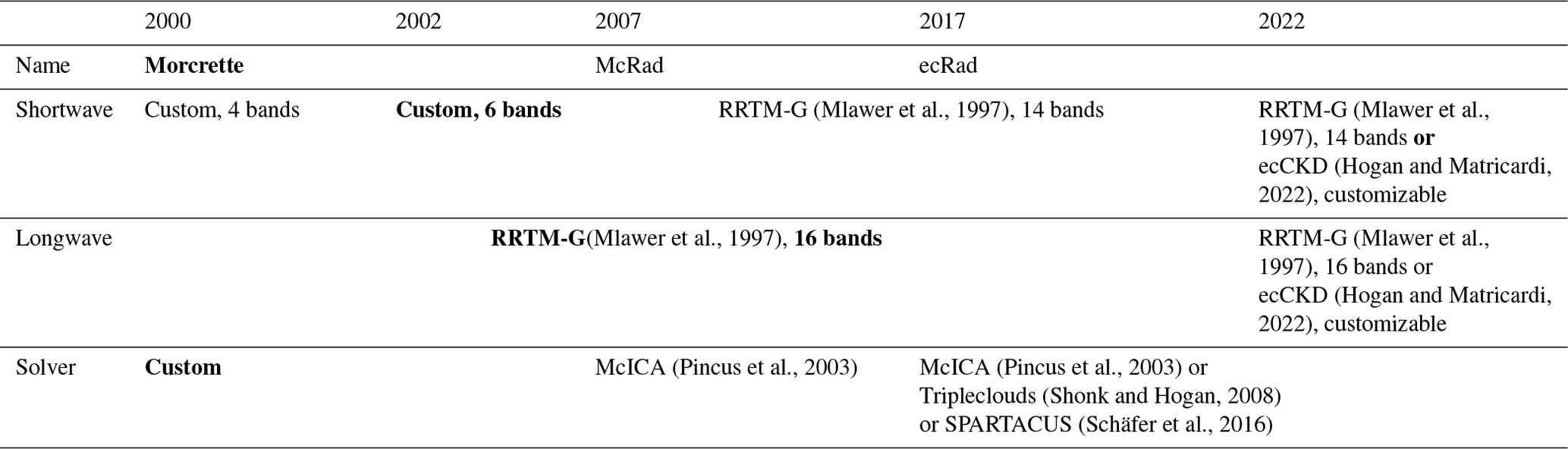
The ecRad radiation scheme is the latest milestone within several decades of development to improve the fidelity of the radiative transfer scheme used within ECMWF’s operational weather prediction model, the IFS. Starting from the 1990s, the IFS used the radiation scheme of Morcrette (1991), which itself went through several updates up to the early 2000s to incorporate various advances in modeling. One major update of the Morcrette scheme was the inclusion, in 2000, of the Rapid Radiative Transfer Model for GCMs (RRTM-G) by Mlawer et al. (1997), a correlated-k model for gas absorption. At the time, RRTM-G was used for longwave radiation only and significantly improved the estimation of surface downward longwave radiation compared to contemporary models (Morcrette, 2002). For shortwave radiation, the Morcrette scheme used a custom gas-optics scheme with four spectral bands in 2000, soon increased to six spectral bands in 2002 (Hogan and Bozzo, 2018). This version was notably used in the ERA-40 reanalysis (Morcrette, 2002; Uppala et al., 2005).

In 2007, the Morcrette scheme in the IFS was replaced by McRad (Morcrette et al., 2008), an improved radiative transfer scheme. In addition to a better representation of surface albedo, this new scheme featured RRTM-G for both shortwave and longwave radiation (with 14 and 16 spectral bands, respectively) and the Monte Carlo Independent Column Approximation (McICA) scheme by Pincus et al. (2003), a radiation solver that simulates clouds with a stochastic generator. Though the McRad radiation scheme was a notable improvement over the Morcrette scheme, its source code was not designed for modularity, making it difficult to include new schemes that act either as alternatives or as improvements over those already provided.

The ecRad radiation scheme by Hogan and Bozzo (2018), which became operational in 2017, provides a more modern modular structure, facilitating inclusion of new advances in atmospheric modeling. Organized in several components through which data flow via dedicated structures, ecRad allows users to swap one scheme with another in each component without breaking the flow of the whole radiative transfer scheme, as illustrated by Fig. 1. Moreover, ecRad manages most of the data required by its inner components with NetCDF files, while the Morcrette scheme still used in MAR relies on hard-coded data, notably for ozone mixing ratios.

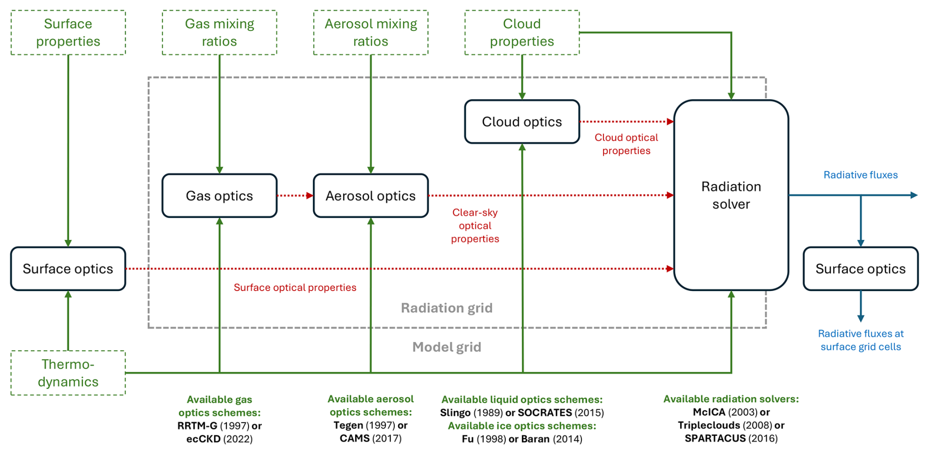
Figure 1 A high-level view of the architecture of the ecRad radiation scheme, inspired by Fig. 1 in Hogan and Bozzo (2018). The rounded and dashed rectangular boxes respectively correspond to ecRad (interchangeable) components and to ecRad inputs. The thermodynamics box corresponds to the temperature and pressure at each layer interface and within each layer. Dashed arrows model the inner ecRad data structures. The background dashed box accounts for the interpolation steps used to go from the model to the radiation grid and vice versa.

Thanks to its flexibility, ecRad provides, among others, several interchangeable schemes to solve radiation equations. In addition to McICA (Pincus et al., 2003), already used by McRad, ecRad also provides the Tripleclouds radiation solver by Shonk and Hogan (2008), which models horizontal cloud inhomogeneity by representing three regions within each grid cell. The more recent SPARTACUS (SPeedy Algorithm for Radiative TrAnsfer through CloUd Sides) scheme is another proposed alternative, capable of simulating 3-D cloud longwave radiative effects (Schäfer et al., 2016; Hogan et al., 2016).

The treatment of the optical properties of gases is another major subcomponent of a radiation scheme that may be experimented with. Both the IFS and the MAR have used the RRTM-G gas-optics scheme for Earth's longwave radiation since the 2000s, with the former also using it for shortwave radiation starting from 2007 with the replacement of the Morcrette scheme by McRad. A promising alternative to this state-of-the-art solution is ecCKD (Hogan and Matricardi, 2022), an open-source tool from the ECMWF that builds fine-tuned gas-optics models via the correlated-k distribution method by Goody et al. (1989), with these models being managed with NetCDF files for convenience. Such a tool can be used to tailor high-resolution gas-optics models for specific applications while remaining computationally efficient.

2.2 Opportunities for the MAR

The MAR is a regional climate model (RCM) consisting of an atmospheric module (Gallée and Schayes, 1994; Gallée, 1995) coupled with SISVAT (Soil–Ice–Snow–Vegetation–Atmosphere–Transfer), a one-dimensional surface transfer scheme (De Ridder and Gallée, 1998; Gallée et al., 2001). This coupling makes MAR a suitable tool to study polar ice sheets, notably in Greenland (Gallée and Duynkerke, 1997; Lefebre et al., 2003, 2005). To compute shortwave and longwave radiative fluxes for its atmospheric module, MAR version 3.13 still uses a late build of the Morcrette scheme (Morcrette, 1991) from 2002 that includes RRTM-G (Mlawer et al., 1997) for longwave radiation (see Table 1). A more complete description of the MAR is provided by Gallée et al. (2013).

(Mlawer et al., 1997)(Mlawer et al., 1997)(Hogan and Matricardi, 2022)(Mlawer et al., 1997)(Mlawer et al., 1997)(Hogan and Matricardi, 2022)(Pincus et al., 2003)(Pincus et al., 2003)(Shonk and Hogan, 2008)(Schäfer et al., 2016)

Table 1 Simplified timeline of the radiation schemes (and their main components) developed by the ECMWF and used in the IFS. A more complete timeline (with more components and code updates) covering the 2000–2017 period can be found in Hogan and Bozzo (2018). The bold elements correspond to the radiation scheme (and components) still used by MAR up to version 3.13.

Used by the ECMWF from the early 1990s to the mid-2000s (Morcrette et al., 2008), the Morcrette scheme is arguably too old to continue using as the radiation scheme of MAR. First of all, it is no longer actively maintained and does not benefit from Fortran language updates from the 2000s that would improve its modularity, such as improved derived types and object-oriented programming mechanisms (Reid, 2007), therefore hindering the implementation of new or improved features. Furthermore, some of its native characteristics are now outdated. For instance, the Morcrette scheme still uses the monthly climatology by Tegen et al. (1997) for tropospheric aerosols, which has little reason to be preferred over more modern climatologies, in particular those using the Copernicus Atmospheric Monitoring Service (CAMS) aerosol specification (Flemming et al., 2017; Bozzo et al., 2017). Finally, another motivation for considering an update of the radiation component of MAR is to eventually improve the radiative fluxes biases. Indeed, MAR with Morcrette is known to have an imbalance between shortwave and longwave radiative fluxes, the former being typically overestimated while the latter is underestimated (Fettweis et al., 2017; Delhasse et al., 2020; Wyard et al., 2018; Kittel et al., 2022).

Including the ecRad radiation scheme in the MAR comes with multiple benefits. Replacing the aging Morcrette scheme by ecRad in MAR is not only a way to modernize MAR itself and an opportunity to fix its known imbalance between shortwave and longwave radiation, but also a way to expand MAR capabilities without requiring any major change in the MAR source code. In particular, the latest version of ecRad (Hogan, 2024a) allows the computation of spectral shortwave radiative fluxes into user-defined bands. Such a development offers new opportunities for the MAR: for instance, the spectral fluxes MAR could output may be used as forcings for other models or as a means of coupling MAR with them. Models that could use such forcings include biogeochemical models designed to study marine ecosystems (Lazzari et al., 2021b).

Another recent key development of ecRad that further motivates this new kind of application of MAR is the ability of ecRad to use high-resolution gas-optics models built with the ecCKD tool (Hogan and Matricardi, 2022) within its gas-optics component (see Fig. 1) in place of the classical RRTM-G scheme by Mlawer et al. (1997). The resulting increase in spectral resolution is especially important. To benefit from the spectral information provided with the new generation of satellites like Sentinel, modern ocean biogeochemical models rely on a refined radiative transfer module that manages spectral bands extending over a few dozen nanometers, e.g., from 400 to 425 nm (Lazzari et al., 2021b, a). This module needs to be forced at the air–sea interface by spectral radiative fluxes, in particular in the wavelength range of photosynthetically active radiation (PAR), i.e., 400–700 nm, but also in the UV and near-infrared ranges. Meanwhile, the (fixed) spectral bands of the RRTM-G gas-optics scheme in ecRad include one band from 442 to 625 nm, which amounts to almost two-thirds of the wavelength range of the PAR, making the RRTM-G gas-optics scheme a poor candidate to compute spectral radiative fluxes in such a range.

Using ecCKD to increase the spectral resolution also comes at a smaller computational cost. Like RRTM-G, ecCKD models define spectral intervals within spectral bands, or “g-points”, to model the spectral variation of gas absorption within bands. The number of such g-points, which has a direct impact on performance, is typically lower in ecCKD models than in RRTM-G (for both shortwave and longwave radiation), even when the former define more spectral bands. As a result, by swapping RRTM-G with high-resolution ecCKD gas-optics models, ecRad can easily output equally high-resolution spectral shortwave fluxes, spanning 1 nm or several dozen nanometers, assuming the bands requested by the user are not finer in resolution. In practice, requesting finer spectral bands than defined in the ecCKD shortwave gas-optics model used by ecRad results in spectral fluxes that are proportional to the encompassing ecCKD spectral band. Therefore, embedding ecRad within MAR and configuring it to run with ecCKD gas-optics models opens the door for new future applications of the MAR as well as for improvements of MAR itself. For instance, high-resolution spectral shortwave fluxes produced by ecRad/ecCKD may be used to implement a spectral snow albedo in MAR.

3 Inclusion of ecRad in MAR

The ecRad radiation scheme (version 1.5.0) is written in Fortran 2003 and consists of about 16 000 lines of code without counting the source code of the RRTM-G scheme (Hogan and Bozzo, 2018). It is also open-source software that comes with excerpts from the IFS source code to show how the IFS initializes then runs ecRad throughout a simulation. While ecRad itself did not require any modification to be embedded in MAR, the source code of MAR needed some adjustments to fully take advantage of the improved representation of optically active components of ecRad as well as its improved spectral resolution.

3.1 Updated greenhouse gas and aerosol forcings

Due to the development history of the ecRad radiation scheme and the IFS (see Sect. 2.1), the example subroutines from the IFS (Hogan, 2024a) share many similarities in terms of interface with the subroutines calling the Morcrette scheme (Morcrette, 1991, 2002) in MAR. Among others, the input variables of the IFS subroutine that calls ecRad include the same description of pressure and temperature profiles as for the Morcrette scheme, and this also holds true for several water species and surface variables (e.g., albedo, emissivity in the longwave, or land–sea mask). However, ecRad natively offers more flexibility regarding greenhouse gases and aerosols. Indeed, for each greenhouse gas or aerosol, ecRad expects the volume or mass mixing ratios for each pressure layer of each air column of the encompassing model grid. The number of aerosol species taken into account by ecRad can also be tuned, with users being able to define up to 256 different species. In comparison, the Morcrette scheme as used by MAR expects a single average mixing ratio for most greenhouse gases and restricts aerosols to six species, as in the climatology of Tegen et al. (1997).

Therefore, to make the most of the ecRad radiation scheme, the greenhouse gases and aerosol forcings of the MAR were updated, re-using climatological data used in the IFS (cycle 46r1). The greenhouse gas forcings consist of 12 monthly 2-D grids providing longitude-averaged mixing ratios for a meridional transect of the Earth’s atmosphere based on reanalyses over the 2000s. For the sake of consistency, the initial volume mixing ratios should be scaled to match the average surface mixing ratios of the year simulated by MAR, with these averages depending on either historical records or future climate scenarios. Such averages can be found in time series of the average surface volume mixing ratio of each greenhouse gas and for each year (from 0 to 2500) according to the Intergovernmental Panel on Climate Change's (IPCC) typical scenarios, the Representative Concentration Pathways (RCPs) (Van Vuuren et al., 2011) and Shared Socioeconomic Pathways (SSPs) (O'Neill et al., 2016). Given a climate scenario time series, the consecutive average surface mixing ratios corresponding to the period covered by the initial forcings are used to compute a period average. Then, the average surface mixing ratio corresponding to the year MAR should simulate is divided by the period average to compute a scaling factor. This scaling factor is then applied to the forcings for the month MAR should simulate. Finally, the scaled forcings are interpolated to the MAR grid and smoothed by averaging with respect to the horizontal axis. This averaging mitigates the jumps in values that are due to the low resolution of the forcings with respect to latitude, as the aforementioned forcings define a total of 64 air columns between the two poles in the meridional transect, with a latitude degree difference between adjacent air columns ranging from 2.8 to 3.2°.

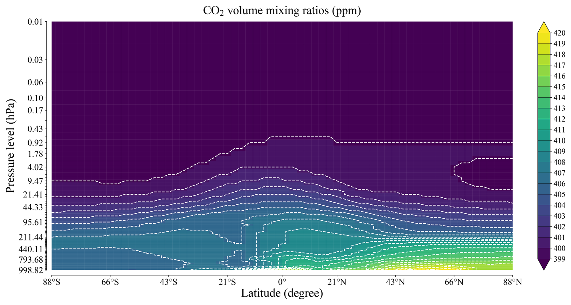
Figure 2 Longitude-averaged volume mixing ratios of CO₂ for a meridional transect of the Earth’s atmosphere for January 2019 (SSP585).

As ecRad is compatible with the CAMS aerosol specification, consisting of 11 hydrophilic or hydrophobic aerosol species (Flemming et al., 2017; Bozzo et al., 2017), the MAR was also updated to provide such forcings to ecRad. Their preparation is essentially the same as for greenhouse gas forcings, the main difference being that the CAMS data provided by the ECMWF (Hogan, 2024b) consist of monthly 3-D grids covering the global Earth’s atmosphere. However, with 61 air columns between the poles in each of the 120 meridional transects with respect to longitude, only a few air columns from the initial forcings will cover the high-resolution MAR grid. Therefore, for the sake of simplicity, the longitude coordinates of the MAR grid are averaged to select the meridional transect within the 3-D CAMS data that is the closest in longitude to the MAR grid. The subsequent steps to prepare the aerosol forcings are then identical to those used to prepare the greenhouse gas forcings.

3.2 Stratospheric layers on top of the MAR grid

As the MAR vertical discretization is usually tuned to simulate the whole troposphere and the lower part of the stratosphere (i.e., slightly above a pressure value of 90 hPa), the impact of the stratosphere on radiative fluxes cannot be properly simulated with the MAR grid alone. This limitation is especially problematic for ozone, which is typically found in greater concentrations in the stratosphere, with significant absorption of incoming solar radiation above 90 hPa, particularly in the ultraviolet range (Hogan and Matricardi, 2020). As one of the motivations for replacing Morcrette by ecRad in MAR is to have a better and finer spectral representation of shortwave radiation (see Sect. 2.2), it is crucial to ensure that the spectral effect of ozone is properly represented. However, adding stratospheric layers to the MAR grid may be counterproductive given the extra computational cost brought by these additional layers. Indeed, as the stratosphere has little water vapor, stratospheric layers have little relevance for the physical processes typically studied with the MAR, such as precipitation, (near-)surface temperature, or snow and ice layers (Fettweis et al., 2013a, 2017; Wyard et al., 2020; Delhasse et al., 2020; Hanna et al., 2020; Amory et al., 2021; Kittel et al., 2022), knowing that the general circulation is forced at its lateral boundaries.

To keep the usual MAR pressure description while simulating the radiative effects of the stratosphere, additional pressure layers are added on top of the MAR grid just before calling ecRad and upon preparing the greenhouse gas and aerosol forcings as described in Sect. 3.1. In other words, the MAR grid is extended with stratospheric pressure layers only during radiation calculations. This means the MAR can run with its usual vertical discretization while still receiving radiative fluxes from ecRad that take account of properties of the stratosphere such as the peak ozone concentration. This also means, however, that some MAR variables fed to ecRad must be set or inferred with respect to the additional stratospheric layers so that they are consistent with real-world observations.

Based on the small water content in the stratosphere and previous work by Hogan and Matricardi (2020), the values of the additional stratospheric layers for the input variables required by ecRad were set as follows. First, it is assumed that there is no cloud, no liquid water, no ice crystals, and no form of precipitation. Second, the top pressure layer of the extended MAR grid must include the stratopause (1 hPa), and the specific humidity in all stratospheric layers is set to $\mathrm{3.1}\times {\mathrm{10}}^{-\mathrm{6}}$ kg kg⁻¹, i.e., the typical median value across the stratosphere according to Hogan and Matricardi (2020), while the vapor saturation threshold is set to the value for 0 °C, i.e., $\mathrm{3.8}\times {\mathrm{10}}^{-\mathrm{3}}$ kg kg⁻¹, to prevent condensation and to stay consistent with the previous assumptions. Finally, it is assumed that the temperature at the stratopause is approximately 60 °C warmer than at the tropopause (Hogan and Matricardi, 2020). For a given air column, the temperature of the stratospheric layers can be inferred by finding the plausible tropopause in the column (which is not necessarily at the top of the said column), adding 60 °C to obtain the temperature at the stratopause, and then linearly interpolating to the intermediate values.

The immediate benefit of adding stratospheric layers on top of the MAR grid is to allow ecRad to capture the radiative effects of the peak concentration of ozone, with the greenhouse gas and aerosol concentrations at the extra pressure layers being prepared using the same method as in Sect. 3.1. The number and limits of the extra pressure layers can be freely configured by MAR users. By default, MAR running with ecRad adds three extra pressure layers on top of the MAR grid, respectively extending from 0 to 5.5 hPa, from 5.5 to 20 hPa, and from 20 to around 50 hPa, this last limit depending on the top of the MAR grid. The greenhouse gas and aerosol concentrations for each of these three layers are adjusted with the concentrations closest to 1 hPa (stratopause), 10 hPa, and 30 hPa (respectively) in the forcings, yielding a total ozone that is close to the total ozone from the forcings when vertically integrated, as shown in Figs. 3 and 4.

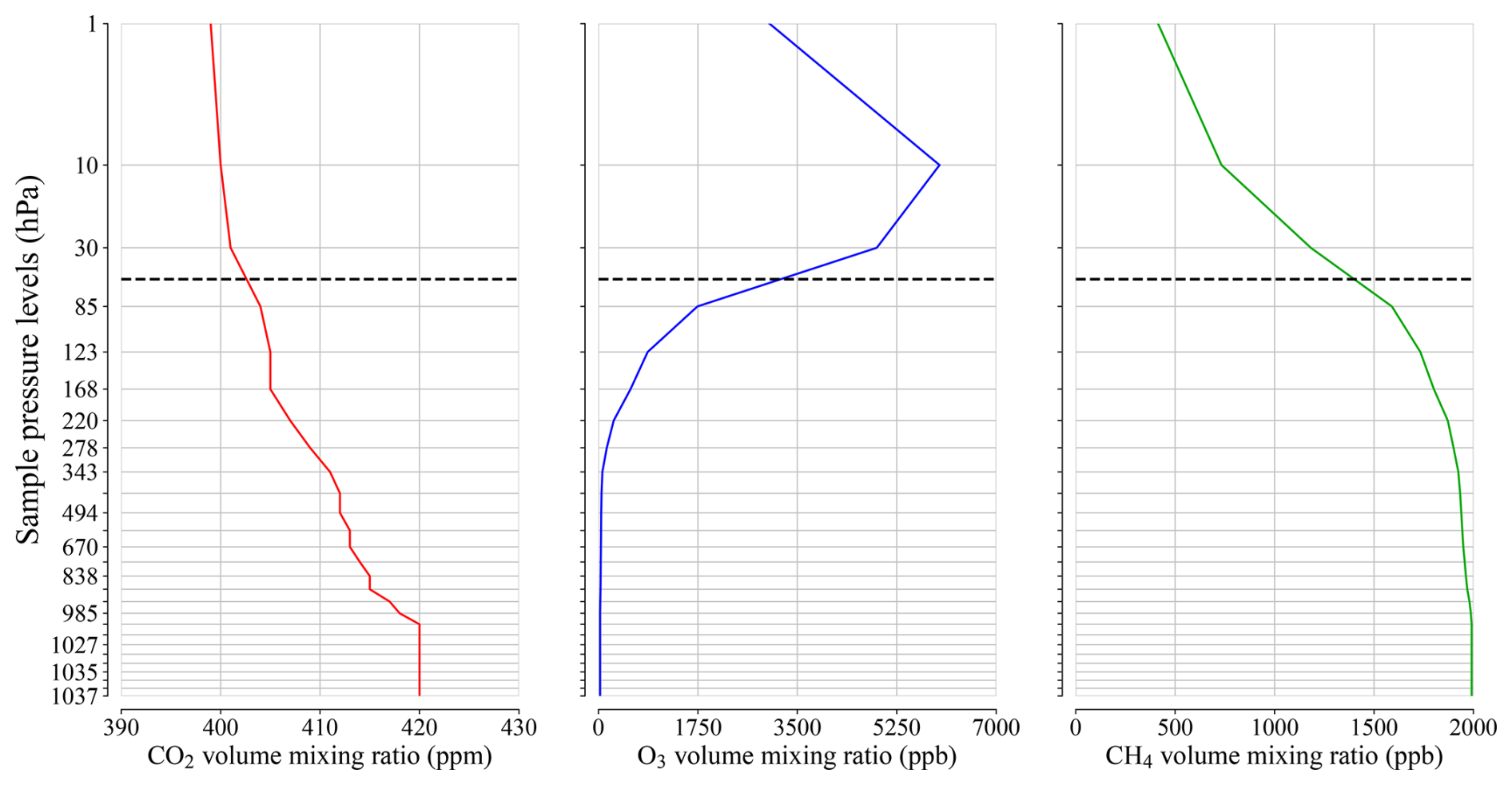
Figure 3 Volume mixing ratios for three greenhouse gases after fitting the forcings (from Fig. 2) to the MAR grid (Sect. 3.1). Due to horizontal smoothing, the mixing ratios only vary vertically. MAR uses sigma coordinates, and the pressure values are based on a representative air column. The dashed line delimits the extra layers added to take account of the radiative effects of the stratosphere (Sect. 3.2).

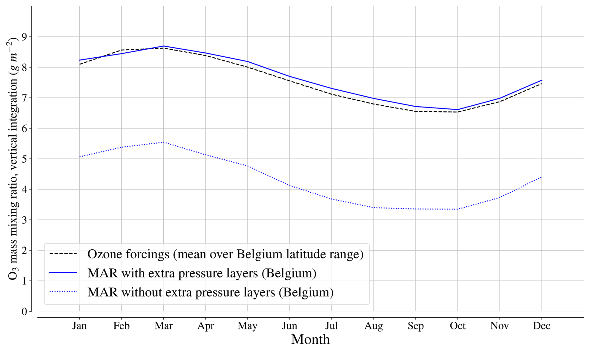
Figure 4 Comparison of the ozone volume mixing ratios fitted to a MAR grid over Belgium before and after adding the extra pressure layers. The mixing ratios are vertically integrated (g m⁻²) and averaged on a monthly basis. The concentrations in the extra layers are adjusted to those found at 1, 10, and 30 hPa. The figure is based on the outputs of a sample MAR v3.14 run over Belgium in 2019.

3.3 Updated cloud fraction parameterization

Clouds are well known for playing a major role in distributing the radiative budget of the Earth (Ramanathan et al., 1989; Shupe and Intrieri, 2004), with direct consequences for surface processes. For instance, by combining climate simulations and satellite observations, Van Tricht et al. (2016) demonstrated that clouds were enhancing ice sheet meltwater runoff in Greenland. Properly representing clouds within a climate model is therefore necessary to compute radiative fluxes that are consistent with real-world observations. When it comes to research involving the MAR, Fettweis et al. (2017) also noted that the biases in the radiative fluxes produced by the Morcrette scheme embedded in MAR were at least partly due to an underestimated cloudiness, with the radiation scheme requiring a cloud fraction value for each grid cell.

While accurately representing clouds within a computer model is a whole research topic of its own (Sundqvist et al., 1989; Xu and Randall, 1996; Tompkins, 2002; Shonk et al., 2010; Weverberg et al., 2013), the prediction of cloudiness in the MAR needed an update to improve the cloud fraction values it feeds to ecRad in order to further improve its output radiative fluxes. Indeed, the code interfacing MAR with the Morcrette radiation scheme still computes cloud fraction values using an old formula from the ECMWF for predicting cloudiness at a large scale. Though this old approach can still be used, the cloud fraction parameterizations from Sundqvist et al. (1989) and Xu and Randall (1996) were added in the MAR code computing the cloud fraction values used by ecRad, with MAR users being able to choose between all three parameterizations.

The parameterizations by Sundqvist et al. (1989) and Xu and Randall (1996) were included in MAR for two reasons. First, recent work by Wang et al. (2022) re-evaluated these with CloudSat data and showed that both parameterizations struggle with predicting cloud vertical structure but are good at predicting the total cloud cover, which is currently the most important requirement for MAR regarding cloudiness, given that research involving the MAR focuses mostly on (near-)surface processes, as previously mentioned in Sect. 3.2. Second, both parameterizations are immediate in terms of implementation, as they only need simple variables from a given grid cell to compute a cloud fraction (CF) for that cell, without considering adjacent cells or grid-wide phenomena. On the one hand, Sundqvist et al. (1989), solely based on relative humidity (RH), use a critical relative humidity threshold (RH_c) to determine a plausible cloud fraction:

$$\begin{array}{}\text{(1)}& \mathrm{CF}=\mathrm{1}-\sqrt{{\displaystyle \frac{\mathrm{1}-\mathrm{RH}}{\mathrm{1}-{\mathrm{RH}}_{\mathrm{c}}}}},\end{array}$$

where the critical threshold depends on the horizontal resolution of the MAR grid in kilometers (dx) and the underlying type of surface (Wang et al., 2022):

$$\begin{array}{}\text{(2)}& {\mathrm{RH}}_{\mathrm{c}}=\left\{\begin{array}{ll}\mathrm{0.7}+\sqrt{\frac{\mathrm{1}}{\mathrm{25}+\mathrm{d}{x}^{\mathrm{3}}}}& \text{if above land}\\ \mathrm{0.81}+\sqrt{\frac{\mathrm{1}}{\mathrm{50}+\mathrm{d}{x}^{\mathrm{3}}}}& \text{above sea}.\end{array}\right.\end{array}$$

On the other hand, the parameterization of Xu and Randall (1996) needs relative humidity (RH), the total mixing ratio (q_t) of non-gaseous water species (i.e., droplets, ice crystals, snowflakes, hail, etc.), the vapor saturation threshold (q_s), and three empirical parameters p, α, and γ:

$$\begin{array}{}\text{(3)}& \mathrm{CF}={\mathrm{RH}}^p\left[\mathrm{1}-\exp (-{\displaystyle \frac{\mathit{\alpha }{q}_{\mathrm{t}}}{{\left[(\mathrm{1}-\mathrm{RH})q_{\mathrm{s}}\right]}^{\mathit{\gamma }}}})\right],\end{array}$$

where p, α, and γ were empirically determined as p=0.25, γ=0.49, and α=100 (Xu and Randall, 1996). Due to their simplicity, the parameterizations by Sundqvist et al. (1989) and Xu and Randall (1996) were preferred over more physically realistic solutions, such as more advanced diagnostic parameterizations (Weverberg et al., 2021b, a) or prognostic solutions (Tompkins, 2002), both requiring more implementation work. The inclusion of these more complex solutions in the MAR is left for future work.

3.4 Default configuration of ecRad in MAR

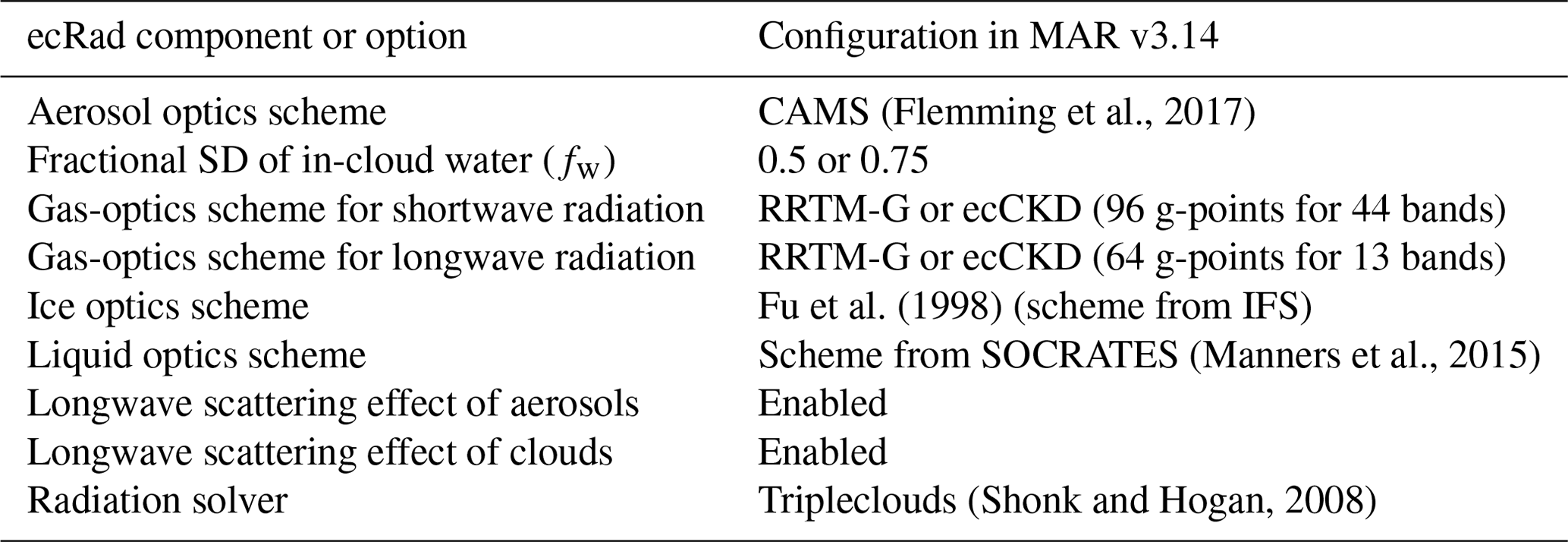
The ecRad radiative transfer scheme includes a large number of options (Hogan and Bozzo, 2018; Hogan, 2024a). To quickly establish a default configuration for MAR, ecRad was configured in MAR with its default or most modern options, which can be reviewed in Table 2. For instance, MAR always enables ecRad to simulate scattering of longwave radiation by clouds, given that such a feature adds an extra computational cost of only 4 % (Hogan and Bozzo, 2018). Likewise, MAR always prepares its aerosol forcings for ecRad with a monthly aerosol climatology compliant with the CAMS aerosol specification (Flemming et al., 2017) rather than the old aerosol climatology of Tegen et al. (1997). With this configuration, MAR can also enable ecRad to simulate the longwave scattering effect of aerosols, an additional process ecRad is unable to perform with the Tegen climatology. While not a option of ecRad, MAR also re-uses the parallelization strategy of the stand-alone implementation of ecRad (Hogan, 2024b, a). It consists of processing one transect of the MAR grid at a time. For each transect, (groups of) air columns are assigned to distinct parallel processes, with the design of ecRad making this strategy very easy to implement.

(Flemming et al., 2017)Fu et al. (1998)(Manners et al., 2015)(Shonk and Hogan, 2008)

Table 2 Configuration of ecRad in MAR v3.14. Options used to design experiments in Sect. 4 are included.

Among the three available solvers in ecRad, the Tripleclouds scheme (Shonk and Hogan, 2008) was picked as the default solver to be used by ecRad in MAR, the McICA scheme (Pincus et al., 2003) being the default solver in ecRad. This choice constitutes a compromise between the research purpose of MAR and the overall computational cost of running ecRad. Indeed, the McICA scheme was designed with operational weather forecasting in mind, while running ecRad with SPARTACUS (Schäfer et al., 2016; Hogan et al., 2016), currently the most advanced of the three solvers, is significantly slower than with both McICA and Tripleclouds (Hogan and Bozzo, 2018). Of course, though Tripleclouds is the preferred radiation solver to be used by ecRad embedded in MAR, MAR users can still configure ecRad to run with any of the available solvers.

Finally, two major parameters of ecRad have been subsequently tuned to design sensitivity experiments in Sect. 4. The first is the gas-optics scheme: due to their novelty, high-resolution gas-optics models built by ecCKD (Hogan and Matricardi, 2022) need to be tested in a regional climate model like MAR before using them as a replacement for the classical RRTM-G scheme (Mlawer et al., 1997). The second is the fractional standard deviation of in-cloud water content, denoted as f_w and defined as the standard deviation of in-cloud water content divided by its mean (Shonk et al., 2010). This parameter controls the inhomogeneity of water content in clouds modeled by the solvers: the smaller f_w is, the more homogeneous clouds will be. Based on multiple data sources, Shonk et al. (2010) recommend using 0.75 ± 0.18, with global climate models in mind. MAR therefore uses 0.75 by default. However, f_w may be set to lower values, such as 0.5, as Table 1 in Shonk et al. (2010) enumerates many f_w values closer to 0.5 than 0.75 for midlatitude or global datasets covering all seasons above land surfaces.

4 Regional evaluation of MAR v3.14 for Belgium

4.1 Methodology

The ecRad radiation scheme has been available in the MAR since version 3.14.0 (Fettweis and Grailet, 2024). For legacy reasons, but also to ease comparison between the new and the old radiation schemes, MAR v3.14 lets users decide whether to use Morcrette or ecRad as the radiation scheme before compilation. As a result, all simulations discussed in this paper were run with MAR v3.14, with some running with the Morcrette scheme and others with ecRad.

Our methodology is as follows. MAR v3.14 has first been configured with the same study domain as Wyard et al. (2017), i.e., a grid centered on Belgium with a resolution of 5 by 5 km and 24 pressure layers in sigma coordinates extending from the surface to the low stratosphere. We then selected the 2011–2020 decade as our period of simulation both to evaluate MAR v3.14 on an extended period and to benefit from the most recent data products of the RMIB. As these data products provide daily values, MAR v3.14 was configured to output daily values as well (means or totals, depending on the variable). The boundary forcings for all simulations have been generated with the ERA5 dataset (Hersbach et al., 2020) for the 2011–2020 decade.

A total of nine simulations have been conducted and are listed with their respective configuration in Table 3. By running nine experiments, each with a unique configuration, we completed two tasks. First, we assessed the climate sensitivity of MAR v3.14 to various configurations of ecRad and established which configuration worked best for Belgium. Second, we evaluated whether or not a well-tuned MAR v3.14 could produce better radiative fluxes with ecRad than with its previous configuration (i.e., still using the Morcrette scheme). In the process, we also assessed if there was any negative impact on other MAR variables.

Table 3 Configurations of all nine MAR (v3.14) simulations discussed in this paper, run over Belgium for the 2011–2020 decade. All experiments with ecRad use the Tripleclouds radiation solver. Each simulation was given a name for the sake of readability.

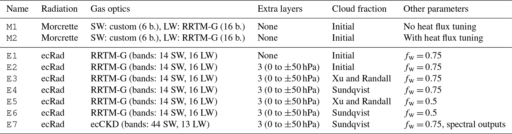
Our first two experiments, M1 and M2, consisted of running MAR v3.14 with the Morcrette scheme without and with a heat flux tuning mechanism inherited from previous versions of MAR, respectively. This tuning mechanism is applied right after heat fluxes have been deduced from the outputs of Morcrette. Historically, this ad hoc mechanism has been implemented in previous MAR versions (up to version 3.13) to slightly mitigate known radiative flux biases with respect to ground observations that have been observed by previous research involving MAR (Fettweis et al., 2017; Wyard et al., 2018; Delhasse et al., 2020; Kittel et al., 2022). By including and tuning ecRad in MAR, we also aim to ensure that MAR no longer needs such a mechanism.

The seven remaining experiments all ran with the ecRad radiation scheme. E1 to E6 have been designed to evaluate not only ecRad itself but also the effects of the additions and parameters discussed in Sect. 3. The first ecRad experiment, E1, simply ran ecRad with its default parameters, briefly discussed in Sect. 3.4, and none of the adjustments described in Sect. 3. Starting from E2, stratospheric pressure layers (Sect. 3.2) are added during radiation calculations, and the next four experiments (from E3 to E6) tested the newly added cloud fraction parameterizations (Sect. 3.3) and two different values of the f_w parameter of ecRad (Sect. 3.4).

The final ecRad experiment, E7, re-used the configuration of E4 but swapped the classical RRTM-G scheme for both shortwave and longwave with high-resolution ecCKD gas-optics models (Hogan and Matricardi, 2022), with two goals in mind. On the one hand, it was meant to verify whether or not swapping RRTM-G with more modern, high-resolution gas-optics models had any negative impact on MAR outputs. On the other hand, E7 was also configured to output spectral shortwave fluxes, whose evaluation and first application, i.e., UV index prediction, are discussed in Sect. 5. For this purpose, the ecCKD models of E7 feature 44 bands in the shortwave and 13 in the longwave. To facilitate accurate calculation of UV index, the former includes 21 bands in the 280–400 nm region. To represent spectral variation of gas absorption within bands, the bands are divided further into g-points such that the total number of quasi-monochromatic spectral intervals is 96 in the shortwave and 64 in the longwave. This is fewer than the 112 and 140 used by RRTM-G in the shortwave and longwave, respectively, resulting in ecCKD being more computationally efficient. It was found that shortwave gas-optics models generated by ecCKD version 1.4 and earlier tended to underestimate surface spectral UV fluxes compared to benchmark line-by-line radiation calculations, which was fixed by increasing the weight of the UV fluxes in the optimization step of the Hogan and Matricardi (2022) algorithm. The shortwave ecCKD model used in this paper is from version 1.6 of ecCKD.

4.2 Evaluation of MAR physical variables

We assess four classical physical output variables of MAR for all nine experiments from Table 3: daily average near-surface (around 2 m a.g.l.) temperature, daily precipitation total, daily mean surface downward shortwave fluxes, and daily mean surface downward longwave fluxes. The first three variables are compared to the gridded products provided by the RMIB, which give daily means or daily totals (in the case of precipitation). These products cover the entire 2011–2020 decade and were built by interpolating ground observations recorded at weather stations scattered across Belgium (Journée and Bertrand, 2010, 2011; Journée et al., 2015). The daily mean downward shortwave fluxes have been further refined by merging the ground observations with satellite measurements provided by the EUMETSAT Satellite Application Facility on Land Surface Analysis (Journée and Bertrand, 2010; Trigo et al., 2011a). The daily mean downward longwave fluxes, i.e., the last of the four assessed MAR physical variables, are directly compared to the MSG daily DSLF dataset (MDIDSLF). This gridded product provides surface downward longwave fluxes as recorded by the successive MSG satellites of EUMETSAT (Trigo et al., 2011a) at 0.05° latitude–longitude resolution over a region covering Europe, Africa, part of South America, and the Middle East. We chose to use this product due to the lack of a gridded RMIB longwave product equivalent to the RMIB shortwave product. According to Trigo et al. (2011b), the DSLF product meets its target accuracy for more than 80 % of its values – that is, a relative error below 10 % compared to land-based observations.

For all experiments and for all variables, the time series for each grid cell from the corresponding RMIB/MSG product is directly compared with the time series from the MAR grid cell that is the closest in geographical coordinates, as all products used feature a nearly identical resolution to the MAR grid. RMIB products have an equivalent resolution of 5 by 5 km grid cells, only on a different projection, while the MSG satellite longwave product has a resolution of 0.05 by 0.05° in latitude and longitude. Once MAR grid cells are paired with comparable grid cells from the data products, the correlation, root mean square deviation (RMSD), and mean difference are computed for each pair of time series. The resulting 2-D statistics have been averaged with respect to the grid and are summarized in Table 4.

Table 4 Evaluation statistics for the main MAR output variables for all experiments from Table 3 and for the 2011–2020 period. All variables, from both MAR and the data products, are (near-)surface daily averages (daily total for precipitation). All statistics are 2-D averages of gridded statistics computed by comparing times series from the reference data (longwave from EUMETSAT MSG satellites, the rest from RMIB) and from the MAR grid points that are the closest in geographical coordinates.

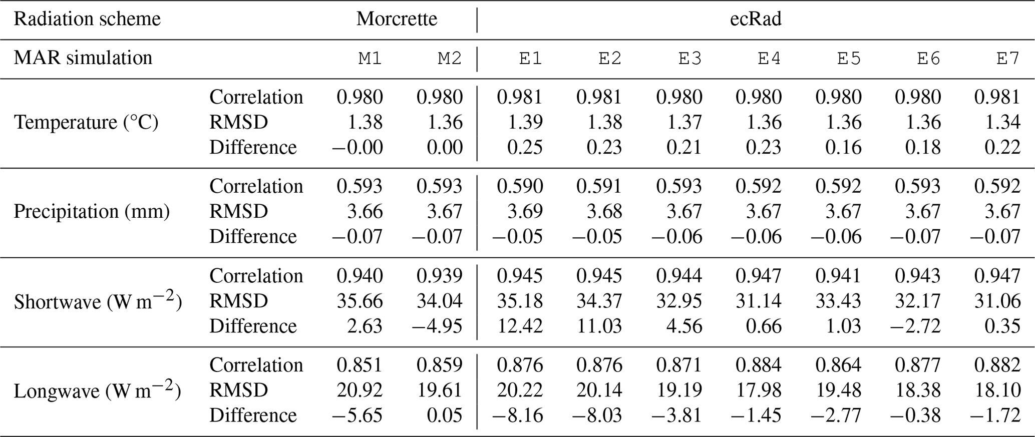
Table 4 demonstrates that all experiments performed well with respect to the RMIB products when it comes to the daily mean temperature and the daily precipitation total: all nine simulations yielded an average correlation over the Belgian territory of around 0.98 for daily mean temperature and of around 0.59 for daily precipitation total. Moreover, the mean differences are fairly low: significantly below 0.3 °C and 0.1 mm in absolute value, respectively.

The average statistics for radiative fluxes have more contrast. While all our experiments yielded good average correlation values, the shortwave flux differences are considerable in some of them. For example, E1, which used none of the adjustments described in Sect. 3, yielded a mean shortwave flux difference of +12 W m⁻². To put this difference into perspective, the average shortwave flux for the whole 2011–2020 decade and for the entire Belgian territory in the RMIB product is about 123 W m⁻². In other words, E1 has almost +10 % more shortwave radiation on average than the RMIB product. Such a large difference would discourage the computation of spectral shortwave fluxes with ecRad embedded in the MAR, which is one of the motivations for including ecRad in MAR in the first place (see Sect. 2.2).

Progressively enabling the adjustments we brought to MAR while transitioning to ecRad (see Sect. 3) steadily improved the mean radiative flux differences, eventually bringing them close to zero on average over Belgium. Starting from E2, radiation calculations in all ecRad configurations take account of three additional stratospheric pressure layers, added on top of the usual MAR grid (using the configuration given in Sec. 3.2). This change reduces the mean shortwave flux difference by almost 1.5 W m⁻², though we expect the additional stratospheric pressure layers to be mostly beneficial to spectral fluxes in the UV range (see Sect. 5). By respectively using the cloud fraction parameterizations of Xu and Randall (1996) and Sundqvist et al. (1989), E3 and E4 reduce their mean differences for both types of radiation with respect to E1 and E2. At the same time, they maintain high correlation values and provide lower root mean square deviations. In particular, E4 brings down the mean shortwave flux difference to near zero, while reducing its mean longwave flux difference with respect to the MSG product to only −1.5 W m⁻². Likewise, E7 provides equivalent results to E4, which means swapping the classic RRTM-G scheme with ecCKD gas-optics schemes for both shortwave and longwave radiation has no negative impact on MAR outputs when it comes to a central Europe region such as Belgium.

Last but not least, E5 and E6 re-use the configurations of E3 and E4 (respectively) but further enhance cloudiness by lowering the value of the f_w parameter in ecRad, which controls the homogeneity of the in-cloud water content (see Sect. 3.4), to 0.5. This lower f_w value falls slightly outside the recommended range of 0.75 ± 0.18 but is also closer to the lower f_w values enumerated in Table 1 in Shonk et al. (2010), which were derived from global or midlatitude datasets covering land surfaces and all seasons. In practice, lowering f_w typically reinforces the radiative effects of clouds in ecRad, as the variability of their water content is brought closer to the mean (see Fig. 1 in Shonk et al., 2010). By lowering f_w with respect to E3 and E4, E5 and E6 further lowered the mean shortwave flux differences, though at the cost of slightly worsening both the correlation and the RMSD. However, both experiments still yielded better mean correlation and RMSD than both M1 and M2 while providing a better radiative balance. In the case of E6, the mean shortwave flux difference even turned negative. In other words, while keeping the default 0.75 value for f_w is sound for Belgium, f_w may be tuned by MAR users to adjust the radiative balance in regions other than Belgium.

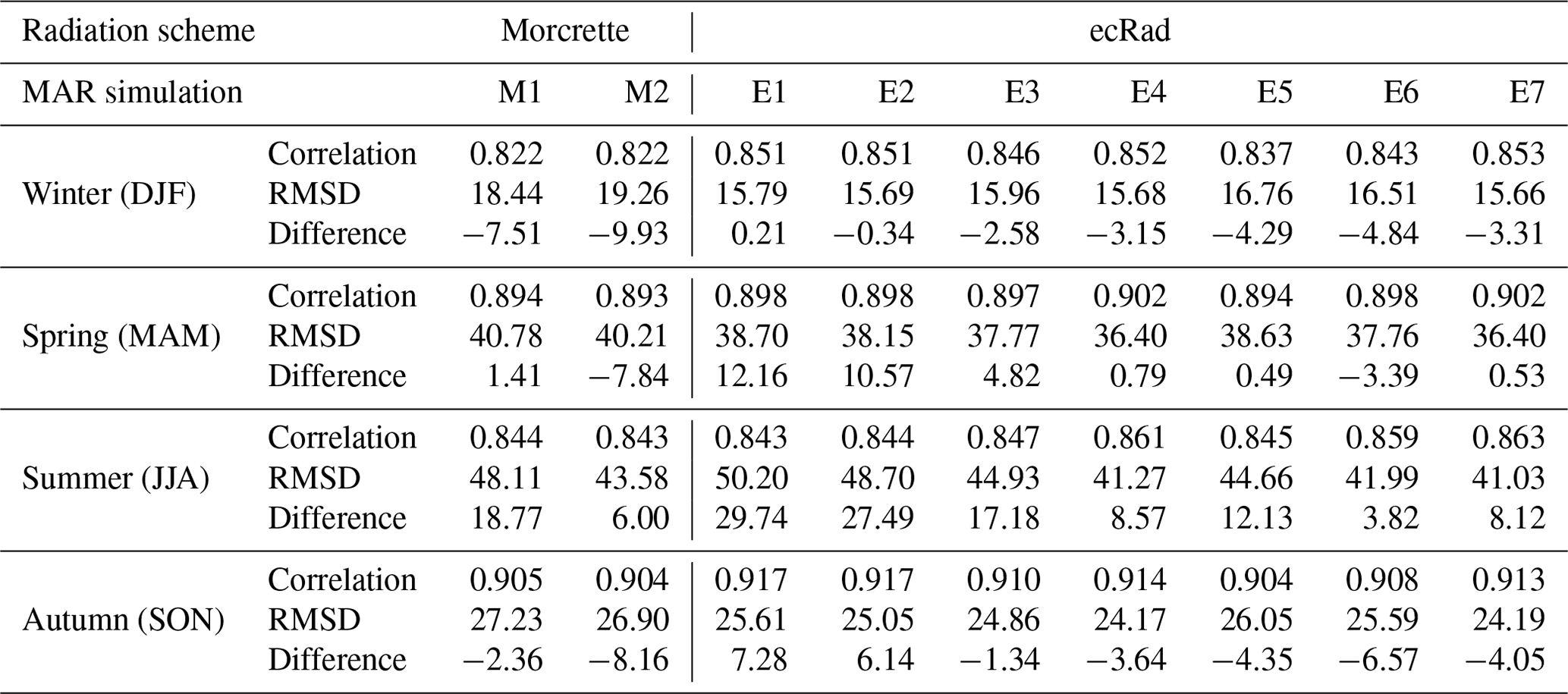
To further analyze the improved shortwave fluxes of MAR v3.14, Table 5 provide seasonal statistics for the daily mean shortwave radiative fluxes for all nine experiments. The statistics are calculated in the same manner as for Table 4, except that the time series are each time-truncated to 3 months corresponding to each of the four seasons, e.g., December, January, and February (DJF) for winter. These seasonal statistics follow similar trends to those observed in Table 4. In particular, the correlation coefficients and root mean square deviations are always better with ecRad, except during the summer for E1, E2, and E3: during this season, M1 and M2 provide equivalent or better results. However, the seasonal statistics for M1 and M2 show non-negligible seasonal disparities regardless of tuning the heat fluxes. In the case of M1, i.e., Morcrette with no tuning, the differences are negligible in spring and autumn but noticeable in the winter and considerable in the summer, with a positive mean difference of almost +20 W m⁻². While M2 brings down the same mean difference to only +6 W m⁻², it is at the cost of worsening the mean differences for all three other seasons. While the two best ecRad experiments (E4 and E7) both have a slightly worse mean difference in summer than M2, at around +8 W m⁻², they provide better statistics for all other seasons in addition to better mean correlations and root mean square deviations for the summer. In conclusion, despite the Morcrette experiments having reasonable mean radiative flux differences in Table 4, the ecRad experiments exhibit a better seasonal behavior.

Table 5 Statistics for the downward shortwave radiative fluxes (daily means) per season for all experiments from Table 3. Again, statistics are 2-D averages of gridded statistics much like in Table 4, but the covered periods are adjusted to the four seasons.

Finally, Figs. 5 and 6 illustrate the spatial variability of the mean shortwave flux differences over Belgium during 2011–2020 for three of our nine experiments: M1 and M2 (Fig. 5), as well as E7 (Fig. 6), respectively. It is worth noting that the spatial variability of the mean shortwave flux differences in all ecRad experiments is roughly the same, though the differences decrease along with the experiments, with E4 providing nearly identical results to E7. Figure 5 demonstrates that the old MAR configuration struggles to produce a grid-wide mean difference close to zero, regardless of tuning the heat fluxes. Indeed, M1, the simulation without tuning the output fluxes, produced an overwhelming majority of positive differences, while M2, which tuned the output fluxes, achieved the opposite result. Figure 6, on the other hand, shows that MAR v3.14 running with the best configuration of ecRad offers low differences for most of the Belgian territory while achieving a grid-wide mean difference of only +0.35 W m⁻². Only the southern tip of Belgium exhibits larger positive differences with E7, though all simulations exhibit their highest differences in that area.

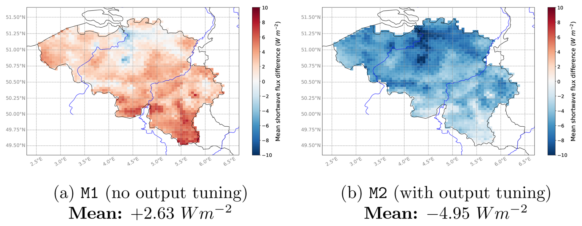
Figure 5 Mean shortwave flux differences of M1 and M2 (MAR v3.14 with Morcrette) for 2011–2020.

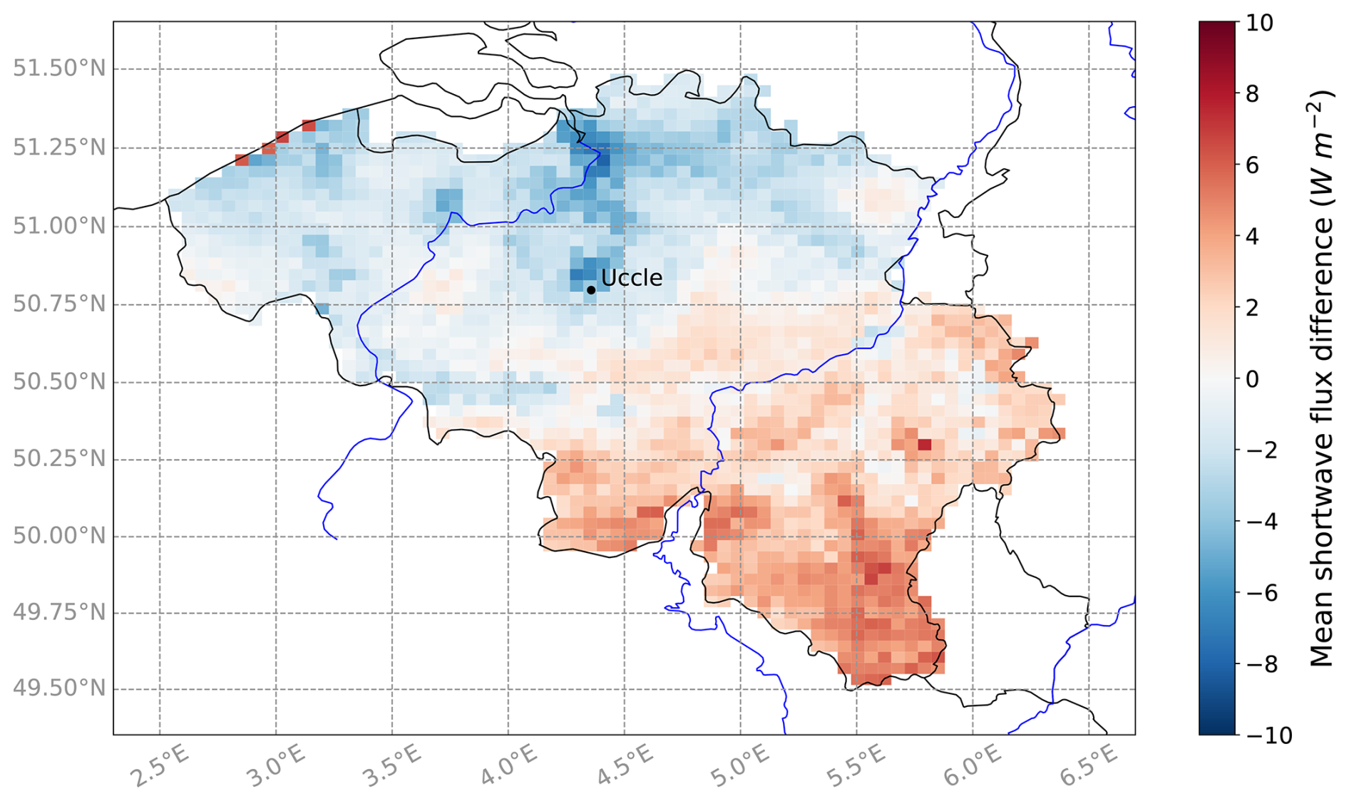
Figure 6 Mean shortwave flux differences of E7 (MAR v3.14 with ecRad and ecCKD) for 2011–2020. The grid-wide mean difference is +0.35 W m⁻². The Uccle location is given for Sect. 5.

4.3 Impact of ecRad on MAR computational performance

To evaluate the cost of all code changes in MAR presented in this paper, the impact on execution time of running MAR with the ecRad radiation scheme instead of the Morcrette scheme should also be assessed. To do so, four representative configurations of the MAR have been run multiple times for a whole day with the Belgium grid (see Sect. 4.1) on the same machine.

The first representative configuration is M2 (see Table 3), which accounts for both simulations running with the Morcrette scheme, as the heat flux tuning mechanism is assumed to have a negligible computational cost. The second assessed configuration is E1, corresponding to the simplest ecRad configuration evaluated in Sect. 4.2. The third one is E4, which accounts for ecRad configurations ranging from E2 up to E6, as all five configurations add the three extra pressure layers during radiation calculations to account for the spectral effects of the stratosphere (see Table 3). These configurations only differ in the choice of the cloud fraction parameterization and the f_w parameter. We also assessed the E7 configuration since the ecCKD schemes are computationally faster than RRTM-G (used by all other ecRad configurations) due to their smaller number of g-points (see Sect. 4.1).

All four configurations have been run on the same machine with an increasing number of CPUs (4, 8, and then 12 CPUs). At each MAR run, the overall execution time was measured with the time command of Linux, while the calls to the radiation scheme were individually timed with the help of the system_clock native Fortran function. To mitigate the randomness of the experiments, notably induced by the varying I/O cost of reading files on disk, each scenario, defined by a configuration and a number of CPUs, has been repeated a total of five times. All recorded times (overall MAR time and ecRad calls) were then averaged for each scenario. Table 6 provides the relative changes in execution time between the ecRad configurations and the Morcrette configurations for each number of CPUs used and on average.

Table 6 Relative changes in time elapsed during ecRad calls with respect to Morcrette calls, both in MAR v3.14, for various ecRad configurations. The M2 configuration was used to assess the performance of the Morcrette scheme. This is based on a single day of simulation (24 calls of the radiation scheme) and using an increasing number of CPUs, with five repetitions.

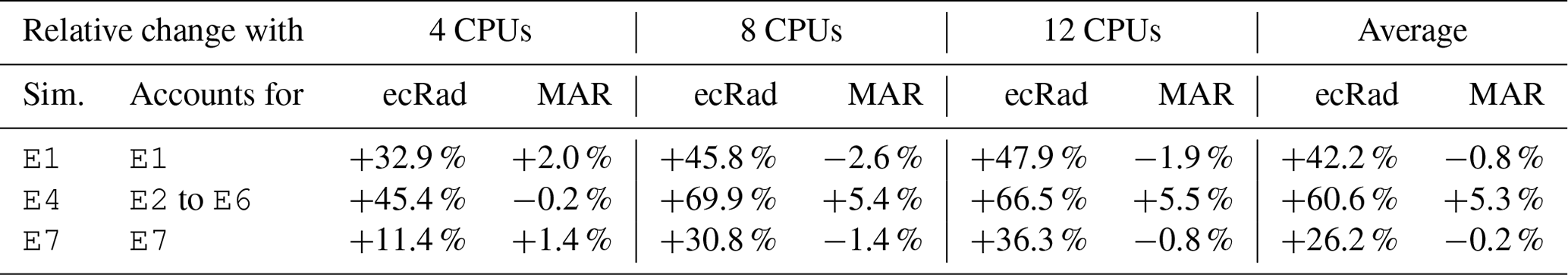
Table 6 shows that running MAR v3.14 with ecRad rather than Morcrette barely has an impact on the overall execution time, with the difference in MAR times ranging from −1.9 to +5.5 %. In practice, the time elapsed during individual radiation calls was under 1 s in all experiments, regardless of the radiation scheme. In other words, even if ecRad calls are up to +70 % longer than Morcrette calls, the extra time is negligible compared to the time elapsed during I/O operations (e.g., reading files on disk), which vary randomly and have a greater cost for MAR overall times in our experiments. Indeed, all lines in Table 6 feature at least one negative relative change for the overall MAR time, regardless of the assessed configuration.

The varying duration of ecRad calls evidenced by Table 6 deserves some commentary. In all configurations, ecRad calls last longer than Morcrette calls. The longer duration of ecRad calls can be attributed to several factors. First of all, all ecRad configurations have a higher spectral resolution for shortwave radiation than the Morcrette configurations (using only six spectral bands; see Sect. 2.1). Second, all ecRad configurations deal with additional physical processes, such as the longwave scattering effect of clouds and aerosols (see Sect. 3.4). Last but not least, with the exception of E1, all ecRad configurations take account of three additional pressure layers during radiation calculations (see Table 3). This addition alone explains the longer ecRad calls of E4 with respect to E1 in Table 6.

The computational burden for ecRad could be reduced by replacing RRTM-G with ecCKD gas-optics schemes, as demonstrated by the E7 line in Table 6: E7 systematically provided the shortest ecRad calls in all experiments. This can be attributed to the lower number of g-points used by the ecCKD models: the two ecCKD models used by E7 feature 96 such g-points in the shortwave and 64 in the longwave, while RRTM-G in ecRad uses 112 and 140 g-points, respectively. In conclusion, running MAR v3.14 with the ecRad radiation scheme has practically no extra cost, especially when ecCKD gas-optics schemes are preferred over RRTM-G.

5 Assessment of spectral shortwave fluxes

5.1 Methodology

From the additional functionality within ecRad and ecCKD gas-optics models, MAR v3.14 is capable of producing fine surface downward spectral shortwave fluxes with user-defined spectral bands, provided the ecCKD algorithm has pre-computed a gas-optics model with a resolution high enough to accommodate the user's bands. As shortly discussed in Sect. 2.2, such a feature offers new research opportunities for the MAR, and we hereby demonstrate its potential by both evaluating spectral shortwave fluxes produced by MAR v3.14 and using the same fluxes for predicting UV indices.

The UV index is a simple metric designed to inform the public about how much harmful ultraviolet radiation reaches the Earth's surface at a given time, as high doses of ultraviolet radiation at specific wavelengths can damage human skin (WHO, 2002). UV indices below 6 correspond to low to moderate risks, while the 6–7 and 8–10 ranges respectively correspond to high and very high risks, with 11 and more, though rare, amounting to extreme danger (WHO, 2002). UV indices are typically obtained by integrating surface downward ultraviolet radiative fluxes in W m⁻² on the 250–400 nm spectral range while weighting them by the action spectrum for erythema, i.e., a redness of the skin that can be induced by solar radiation, as defined by ISO/CIE (1999). In particular, this spectrum gives more weight to the 250–328 nm range. Given the CIE action spectrum s_er(λ), which returns a weight given a wavelength λ expressed in nanometers (nm), the UV index I_UV is defined as

$$\begin{array}{}\text{(4)}& I_{\mathrm{UV}}=\mathrm{40}\times \underset{\mathrm{250}}{\overset{\mathrm{400}}{\int }}{s}_{\mathrm{er}}\left(\mathit{\lambda }\right)f_{\mathrm{sw}}\left(\mathit{\lambda }\right)\mathrm{d}\mathit{\lambda },\end{array}$$

where f_sw(λ) denotes the surface downward shortwave radiative flux in W m⁻² at a given wavelength λ in nanometers (nm) and where the product s_er(λ)f_SW(λ) is also called the erythemal irradiance (McKenzie et al., 2014).

To both evaluate the spectral fluxes produced by MAR v3.14 and use them to predict UV indices, the Royal Belgian Institute for Space Aeronomy, or BIRA-IASB (for Koninklijk Belgisch Instituut voor Ruimte-Aeronomie–Institut royal d'Aéronomie Spatiale de Belgique), provided us with spectral measurements captured by a spectrometer at Uccle (50.797° N, 4.357° E; see Fig. 6) from late June 2017 to December 2020. These measurements, given in $\mathrm{mW}{\mathrm{m}}^{-\mathrm{2}}{\mathrm{nm}}^{-\mathrm{1}}$, cover the 280–500 nm spectral range with a step of 0.5 nm and have been captured every 15 min during daytime. They are not continuous across the covered period, as they have been sporadically interrupted, and as a few days had to be omitted due to calibration issues. The 280–500 nm range covers both the UV-A and UV-B ranges (Tobiska and Nusinov, 2006) and most of the range covered by the CIE action spectrum for erythema, i.e., 250–400 nm (ISO/CIE, 1999); note that virtually no radiation in the range 250–280 nm penetrates to the surface due to being completely absorbed by ozone (Hogan and Matricardi, 2020). The spectrometer also covers a third of the wavelength range of the photosynthetically active radiation (PAR), defined as 400–700 nm.

To compare MAR v3.14 with the spectral observations from Uccle, the E7 experiment from Table 3 (Sect. 4.1), running ecRad with high-resolution ecCKD gas-optics models, has been configured to also produce hourly spectral shortwave fluxes in W m⁻². ecRad maps the surface spectral fluxes from internal shortwave bands (determined by the ecCKD gas-optics model in use) to user-specified output bands, assuming that the optical properties of the atmosphere are constant across each internal shortwave band. Therefore, the spectral distribution of radiation within each band is proportional to the incoming solar spectrum at the top of the atmosphere. This means that if the user requests much finer spectral output than is resolved internally, the spectral outputs may not be accurate, even though they will integrate to the same broadband shortwave flux.

In our case, we configured a total of 29 output spectral bands in our E7 experiment: 14 consecutive 5 nm wide bands covering the 280–350 nm range (i.e., 280–285, 285–290, 290–295, etc.) and 15 consecutive 10 nm wide bands for the 350–500 nm range. These bands are defined almost identically among the 44 spectral bands from the 96 g-point ecCKD model for shortwave radiation used by E7 (see Sect. 4.1). As a result, there is no significant error incurred by the mapping between the ecCKD spectral bands and the requested spectral bands. Moreover, the 14 first bands each cover a smaller range to ensure that the UV-B range and the lower part of the UV-A range are well captured enough for UV index prediction, with the part of the CIE action spectrum having the most impact on UV indices ranging from approximately 280 to 310 nm (McKenzie et al., 2014).

5.2 Evaluation of spectral fluxes at Uccle

To evaluate the spectral shortwave fluxes of the E7 MAR v3.14 simulation, we post-process the BIRA-IASB spectral data from Uccle into a format suitable for direct comparison. This post-processing is done in two steps. The first step consists of numerically integrating the BIRA-IASB data on the spectral bands we defined on the 280–500 nm range in E7. Given U_sw(λ), a raw spectral observation from Uccle at the λ wavelength (by steps of 0.5 nm) and given in $\mathrm{mW}{\mathrm{m}}^{-\mathrm{2}}{\mathrm{nm}}^{-\mathrm{1}}$, the numerical integration $I_{{\mathit{\lambda }}_{\min },{\mathit{\lambda }}_{\max }}$ on the MAR spectral band λ_min−λ_max nm in W m⁻² is given by

$$\begin{array}{}\text{(5)}& I_{{\mathit{\lambda }}_{\min },{\mathit{\lambda }}_{\max }}=\sum _{i=\mathrm{0}}^N{\displaystyle \frac{U_{\mathrm{sw}}({\mathit{\lambda }}_{\min }+\mathrm{0.5}\times i)}{\mathrm{1000}}}\times \mathrm{0.5},\end{array}$$

where N is $({\mathit{\lambda }}_{\max }-{\mathit{\lambda }}_{\min })\times \mathrm{2}-\mathrm{1}$. Once all Uccle measurements have been numerically integrated on our 29 spectral bands, the second step simply consists of aggregating the resulting spectral bands for a given date and hourly slot and computing the hourly average flux per band in W m⁻². Doing so, the post-processed Uccle data have the same temporal and spectral resolution as the MAR spectral fluxes. Finally, it should be noted that, upon calling a radiation scheme for a given hour, MAR prepares the cosine of the solar zenith angle at the half-hour to get representative fluxes for the hourly slot. Therefore, to guarantee that sunrise and dusk happen at the same time in both datasets, the Uccle times were shifted by half an hour just before computing the hourly average spectral fluxes.

We then compare the time series of spectral shortwave downward fluxes (produced by E7) from the MAR grid cell encompassing the geographical coordinates of Uccle with the post-processed Uccle data. Since the latter are not a completely continuous time series and consists exclusively of daylight measurements, the former have been truncated to only feature common hours. As a consequence, nocturnal time steps from MAR are omitted from our evaluation. Table 7 provides, for each spectral band, the mean and standard deviation of Uccle fluxes in W m⁻² followed by the correlation, root mean square error (RMSE), and bias of the MAR spectral fluxes for the same band. To visually compare our spectral fluxes to the post-processed Uccle data, Fig. 7 plots the mean and standard deviation for each MAR spectral band for both the post-processed Uccle spectral observations and MAR spectral fluxes as a function of the wavelength and re-expressed in $\mathrm{mW}{\mathrm{m}}^{-\mathrm{2}}{\mathrm{nm}}^{-\mathrm{1}}$ to ensure that the shapes of the average curves match the magnitudes of the solar radiation reaching Earth's surface.

Table 7 Evaluation statistics of MAR spectral shortwave downward fluxes for each spectral band defined in Sect. 5.1 compared to daytime measurements recorded at Uccle between June 2017 and December 2020 that were numerically integrated on the same spectral bands. Only common dates and hours are compared. The values for the first two bands (italic) are considered noise because the spectrometer is unable to measure fluxes below 10⁻³ $\mathrm{mW}{\mathrm{m}}^{-\mathrm{2}}{\mathrm{nm}}^{-\mathrm{1}}$, which amounts to $\mathrm{5}\times {\mathrm{10}}^{-\mathrm{6}}$ W m⁻² for a 5 nm wide band. The elements in bold font correspond to the sum of all bands in 280–500 nm.

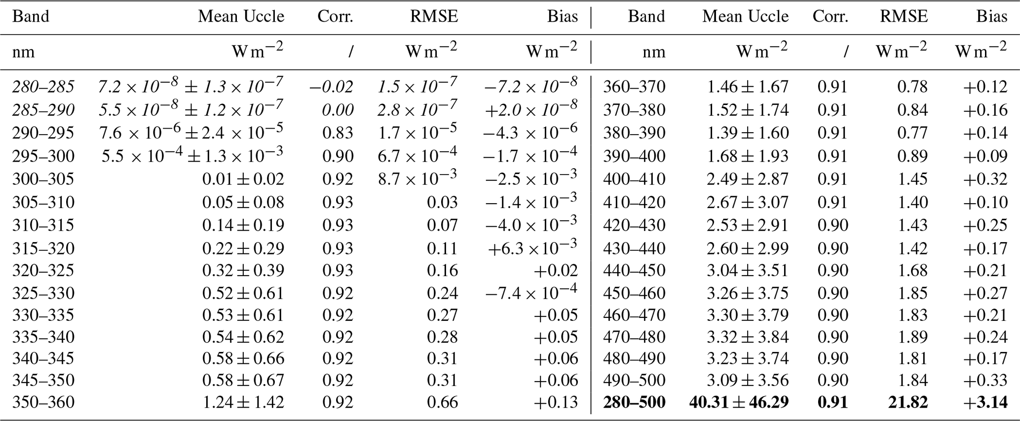
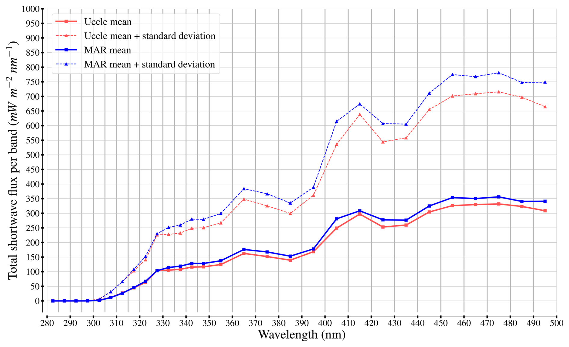
Figure 7 Mean and standard deviation of the spectral shortwave fluxes derived from Uccle observations (June 2017 to December 2020, daytime only) and from MAR v3.14 (E7 from Table 3). The x axis gives the wavelengths, while the y axis gives the fluxes in $\mathrm{mW}{\mathrm{m}}^{-\mathrm{2}}{\mathrm{nm}}^{-\mathrm{1}}$. The mean and standard deviation of each band from both sources were computed on a total of 11 848 comparable time steps.

Table 7 and Fig. 7 both demonstrate a strong correlation between the daytime observations from Uccle and the (daytime) spectral outputs of our E7 simulation. Only the first two spectral bands have a near-zero correlation, but this can be attributed to the spectrometer being unable to record fluxes below 10⁻³ $\mathrm{mW}{\mathrm{m}}^{-\mathrm{2}}{\mathrm{nm}}^{-\mathrm{1}}$, which amounts to $\mathrm{5}\times {\mathrm{10}}^{-\mathrm{6}}$ W m⁻² for a 5 nm wide band. As such, the spectral fluxes recorded between 280 and 290 nm may be considered noise rather than real observations. Starting from 290 nm, MAR spectral fluxes start to correlate well with the post-processed Uccle observations, with the correlation rising to 0.93 at the end of the UV-B range, which ends at 315 nm (Tobiska and Nusinov, 2006). Starting from 315 and until 500 nm, the correlations remain strong but the biases and root mean square errors rise along the mean Uccle spectral fluxes. Figure 7 highlights this very well, as it simultaneously depicts a nearly perfect match between the MAR spectral fluxes and the post-processed Uccle fluxes for the UV-B range (280–315 nm) and consistently positive biases of MAR spectral fluxes for the rest of the spectrum, though these biases always stay below 50 $\mathrm{mW}{\mathrm{m}}^{-\mathrm{2}}{\mathrm{nm}}^{-\mathrm{1}}$ (which amounts to 0.5 W m⁻² for a spectral band of 10 nm).

The consistent biases of our E7 experiment in the 315–500 nm range may be explained by an underestimated cloudiness in MAR. To investigate these biases, we assess MAR cloudiness with the help of an hourly binary cloudiness mask (i.e., 1 for a cloudy sky, 0 otherwise) over Uccle for the 2017–2020 period from the CLAAS-3 dataset of the EUMETSAT Satellite Application Facility on Climate Monitoring (CM SAF) (Benas et al., 2023). To find days that are cloudy in both MAR and the CM SAF observations, we use the daily mean total cloud cover variable of the former, restricted to the grid cell closest to Uccle, and compute daily means of the binary mask from the latter. We then filter both time series to find days where both the MAR daily mean cloud cover and the CM SAF daily mean cloud cover are above 0.7. Using the same time series and the same threshold values, we also find days that are cloudy in the CM SAF observations but only partly cloudy or clear in MAR.

Figure 8 plots the mean and standard deviation for each spectral band we defined in the 280–500 nm range in the same manner as Fig. 7 but after filtering the data on the basis of the aforementioned cloud cover time series. In the left panel, the spectral observations and corresponding MAR fluxes are restricted to days deemed cloudy by both the MAR and the SAF observations. In the right panel, on the other hand, the spectral observations and MAR fluxes are restricted to days that are cloudy in SAF observations but partly cloudy or clear in MAR. When the MAR is in agreement with the CM SAF observations, the spectral flux biases of the former become negligible in the 280–400 nm range and only noticeable within specific bands beyond the 400 nm wavelength. Conversely, when MAR deems a day to be less cloudy than it is in the CM SAF observations, the bias can rise to almost +100 $\mathrm{mW}{\mathrm{m}}^{-\mathrm{2}}{\mathrm{nm}}^{-\mathrm{1}}$ towards the higher wavelengths as a consequence of the underestimated cloudiness. In other words, for a single 10 nm wide band, the bias from MAR can rise to almost +1 W m⁻².

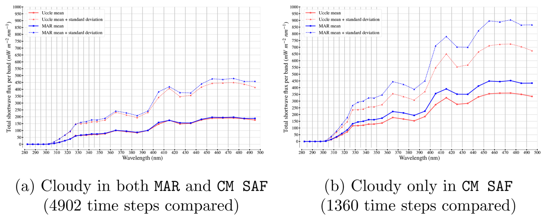
Figure 8 Mean and standard deviation of the spectral shortwave fluxes derived from Uccle observations (June 2017 to December 2020) and from MAR v3.14 (E7 from Table 3) after filtering the data to only keep cloudy days. A day is deemed cloudy when the daily average cloud cover (from either MAR or the hourly CM SAF binary cloudiness mask) is greater than 0.7.

The large spectral flux biases highlighted by Fig. 8 are partly mitigated in Fig. 7, where all spectral observations are considered, due to the number of time steps where MAR is in disagreement with the CM SAF observations making up less than 10 % of the total number of comparable time steps, i.e., 1360 time steps out of a total of 11 848. In comparison, there are almost 4 times more time steps where MAR agrees with the cloudy days from CM SAF, i.e., 4902 time steps. The large differences in magnitude between the two plots in Fig. 8 also hint at when the MAR struggles with cloudiness. Among the 1360 time steps where MAR underestimates the total cloud cover with respect to the CM SAF observations, 721 (approximately 53 %) belong to summer months, i.e., June, July, and August, with 358 (around 26.3 %) just for the July months during 2017–2020. In other words, MAR underestimates cloudiness particularly in the summer, when shortwave fluxes are the strongest in Belgium, which may explain the positive summer shortwave flux differences given in Table 5, as well as the shortwave spectral flux biases given in Table 7 and pictured by Fig. 7.

5.3 A first application: UV index prediction

The very good agreement between the spectral shortwave fluxes of our E7 experiment and the Uccle spectral observations in the UV-B range (i.e., 280–315 nm) makes MAR v3.14 running with ecRad a credible candidate for predicting UV indices. Therefore, we hereby apply the concept of the UV index to both the Uccle spectral observations and the shortwave spectral fluxes from E7. While the BIRA-IASB did not provide us with UV index data from Uccle over the same period as the spectral observations, the high resolution of these observations, which measured shortwave radiative fluxes per steps of 0.5 nm, should lead to realistic UV indices. We can therefore compare the UV indices derived from the observations to the indices predicted on the basis of MAR spectral fluxes to assess whether or not MAR v3.14 can predict credible UV indices while defining a few dozen spectral bands, assuming these spectral bands are not finer than the spectral resolution of the ecCKD gas-optics model for shortwave radiation used internally by ecRad.

As explained in Sect. 5.1 and formulated in Eq. (4), the UV index is essentially an integration of surface ultraviolet radiative fluxes in W m⁻² on the 250–400 nm spectral range weighted by the CIE action spectrum (ISO/CIE, 1999). The CIE action spectrum for erythema s_er(λ) is formally defined as

$$\begin{array}{}\text{(6)}& s_{\mathrm{er}}\left(\mathit{\lambda }\right)=\left\{\begin{array}{ll}\mathrm{1.0}& \text{if}\mathit{\lambda }\in [\mathrm{250},\mathrm{298}]\mathrm{nm}\\ {\mathrm{10}}^{\mathrm{0.094}(\mathrm{298}-\mathit{\lambda })}& \text{if}\mathit{\lambda }\in ]\mathrm{298},\mathrm{328}]\mathrm{nm}\\ {\mathrm{10}}^{\mathrm{0.015}(\mathrm{140}-\mathit{\lambda })}& \text{if}\mathit{\lambda }\in ]\mathrm{328},\mathrm{400}]\mathrm{nm},\end{array}\right.\end{array}$$

where λ is a wavelength expressed in nanometers (nm) in the 250–400 nm spectral range (ISO/CIE, 1999; McKenzie et al., 2014). Although both the Uccle measurements and the spectral bands we configured in the E7 experiment begin at 280 nm, the 250–280 nm spectral range is expected to have little impact on UV indices due to radiation from the UV-C spectral range (100–280 nm) being completely absorbed by the ozone layer (Tobiska and Nusinov, 2006; Hogan and Matricardi, 2020). In other words, the most relevant ranges for UV index prediction are the UV-B range and the beginning of the UV-A range, on which E7 is in very good agreement with the numerically integrated Uccle observations (see Sect. 5.2).

Since both the Uccle spectral observations and the MAR spectral fluxes are provided in small, fine spectral bands, though the former has a higher resolution than the latter, we can predict UV indices by performing the numerical equivalent of the continuous integration (Eq. 4). In other words, we will compute UV indices as weighted sums of our spectral fluxes, the weights being defined by the CIE action spectrum formally defined by Eq. (6).

The UV indices derived from Uccle observations are calculated as follows. First, we numerically integrate the raw measurements between 280 and 400 nm on 1 nm wide bands in order to eliminate the factor of 2 between the initial measurements (by steps of 0.5 nm) and their unit ($\mathrm{mW}{\mathrm{m}}^{-\mathrm{2}}{\mathrm{nm}}^{-\mathrm{1}}$) before averaging the fluxes on an hourly basis, again to match the temporal resolution of MAR. Then, the UV indices based on Uccle data are obtained by computing the numerical equivalent of Eq. (4). The UV indices based on the spectral shortwave fluxes produced by our E7 experiment are calculated mostly in a similar manner, except that we compute for each MAR spectral band an average CIE action spectrum weight $W_{{\mathit{\lambda }}_{\min }}^{{\mathit{\lambda }}_{\max }}$ as

$$\begin{array}{}\text{(7)}& W_{{\mathit{\lambda }}_{\min }}^{{\mathit{\lambda }}_{\max }}={\displaystyle \frac{\mathrm{1}}{{\mathit{\lambda }}_{\max }-{\mathit{\lambda }}_{\min }}}\times \sum _{\mathit{\lambda }={\mathit{\lambda }}_{\min }}^{{\mathit{\lambda }}_{\max }-\mathrm{1}}{s}_{\mathrm{er}}\left(\mathit{\lambda }\right),\end{array}$$

where λ_min and λ_max respectively denote the lower and upper bounds of a MAR spectral band defined on the λ_min–λ_max nm range. With $W_{{\mathit{\lambda }}_{\min }}^{{\mathit{\lambda }}_{\max }}$ defined, UV indices based on E7 are calculated with

$$\begin{array}{}\text{(8)}& \begin{array}{rl}{I}_{\mathrm{UV}}& =\mathrm{40}\times \left[\sum _{i=\mathrm{1}}^{\mathrm{14}}{W}_{\mathrm{280}+\mathrm{5}(i-\mathrm{1})}^{\mathrm{280}+\mathrm{5}i}{M}_{\mathrm{sw}}\left(i\right)\right.\\ & \left.+\sum _{i=\mathrm{15}}^{\mathrm{19}}{W}_{\mathrm{350}+\mathrm{10}(i-\mathrm{15})}^{\mathrm{350}+\mathrm{10}(i-\mathrm{14})}{M}_{\mathrm{sw}}\left(i\right)\right],\end{array}\end{array}$$

where M_sw denotes a spectral shortwave flux produced by our E7 experiment in W m⁻² and where i denotes one of the 19 consecutive spectral bands over 280–400 nm tuned in E7 and exhaustively enumerated in Table 7 (Sect. 5.2).

Using the numerical equivalent of Eq. (4) and the formulas presented in Eqs. (7) and (8), UV indices can be computed offline directly from the BIRA-IASB data and the E7 spectral fluxes. We compare the time series of the UV indices respectively derived from the BIRA-IASB data and from the E7 shortwave spectral fluxes from the MAR grid cell encompassing Uccle in the same way as we previously did for the spectral bands, i.e., by keeping only common dates and hours and computing the correlation, root mean square error, and bias. Doing so, we obtain a correlation of 0.93, an RMSE of 0.656, and a bias of +0.043. When it comes to the extreme values, the observations yield a maximum UV index of 9 (9.161) versus a maximum UV index of 8 (8.117) yielded by the E7 spectral outputs. In other words, UV indices based on MAR v3.14 spectral outputs closely match the indices derived from the BIRA-IASB data, the main issue being that the former fall short of capturing the maxima of the latter. Figure 9 allows visualizing both these observations by plotting the daily average UV index (based on hourly indices between 10:00 and 16:00) from both time series on the year 2019, i.e., the most complete year in the BIRA-IASB data. Indeed, the MAR curve matches the observation curve quite well, excluding the days with missing data, but misses several of its spikes.

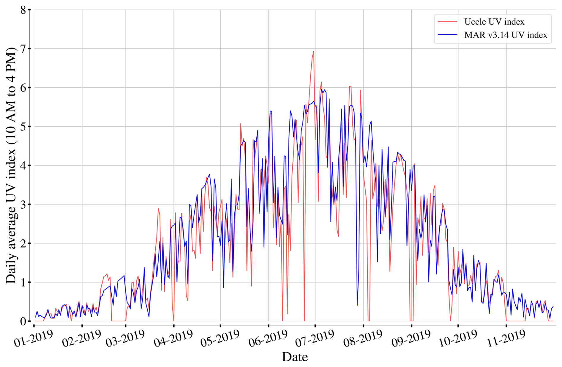
Figure 9 Daily average UV index (based on hourly indices between 10:00 and 16:00 UTC) at Uccle respectively based on the BIRA-IASB data and the E7 spectral shortwave fluxes (MAR v3.14) during the year 2019 (the most complete year in BIRA-IASB data).

To explore the differences between the UV indices derived from the observations and from MAR v3.14 spectral fluxes (E7), Fig. 10 provides the mean and standard deviation for erythemal irradiance as a function of the wavelength for both the Uccle data and the E7 fluxes. Contrary to Figs. 7 and 8, the differences in resolution are represented, as the UV indices based on Uccle data are calculated on the basis of nanometer-wide spectral bands. While both curves match well in the 280–300 and 325–400 nm spectral ranges, non-negligible differences appear in between, with the maxima (in mean only or with standard deviation) belonging to the Uccle curve. For instance, in the middle of the 300–310 nm range, the erythemal irradiance is noticeably higher with Uccle observations, with this part of the 300–325 nm range having slightly more weight in UV index calculation than higher wavelengths in the same range. This slight underestimation from MAR may be a consequence of mismatch between the total ozone during the observation period and the total ozone in MAR (see Sect. 5.4).

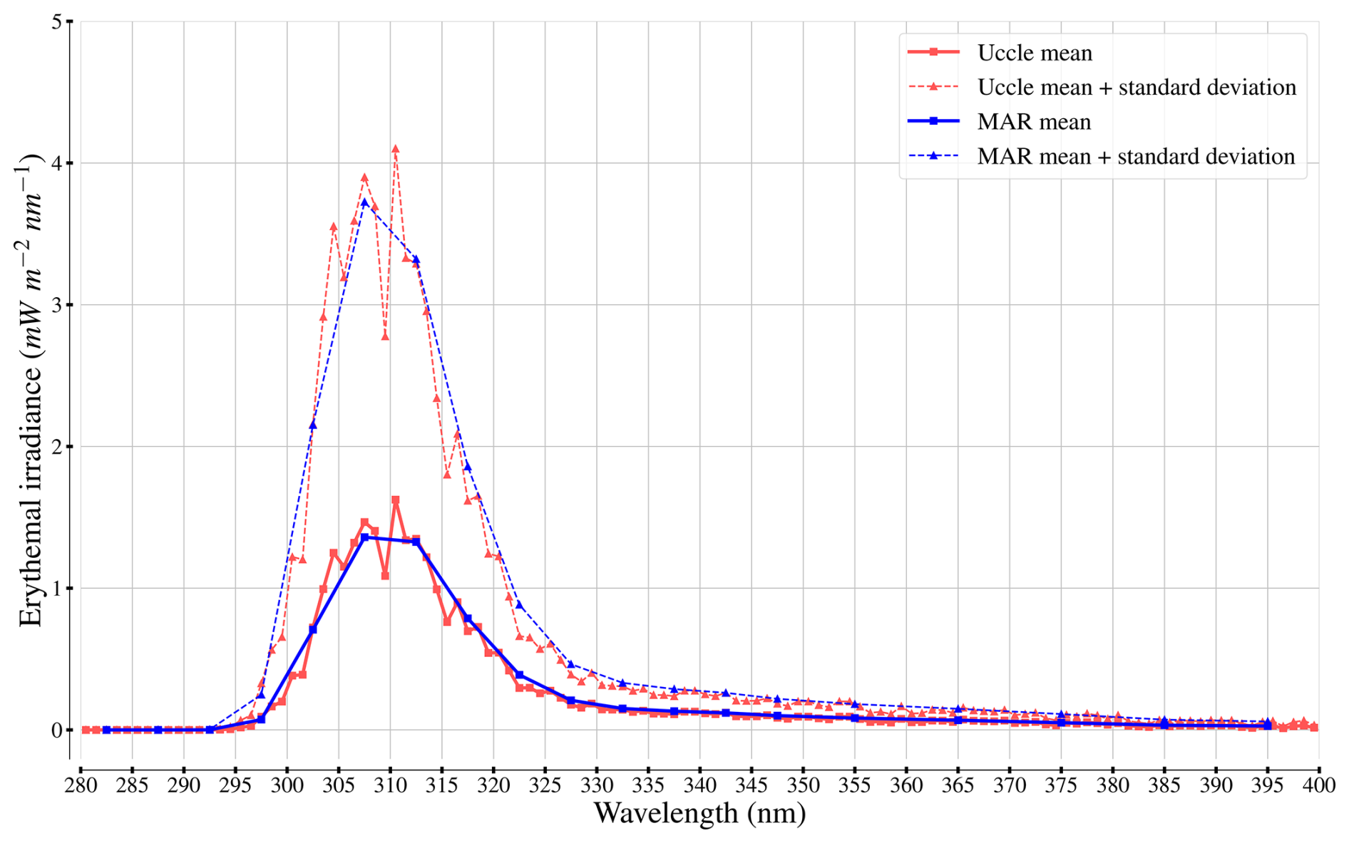
Figure 10 Mean and standard deviation for erythemal irradiance (i.e., shortwave radiative fluxes weighted by the CIE action spectrum for erythema; McKenzie et al., 2014) as a function of the wavelength for both Uccle data and the E7 experiment (June 2017 to December 2020).

5.4 Discussion

Our evaluations of both the simulated physical variables and the spectral shortwave fluxes of MAR v3.14 allow us to gauge the benefits of including the ecRad radiative transfer scheme and to assess the current limits of MAR v3.14. Table 5 from Sect. 4.2 and Figs. 7 and 8 show that radiative flux biases remain across seasons due to underestimation or overestimation of cloudiness, depending on the season. As highlighted in Sect. 5.2 (with the help of Fig. 8), MAR struggles to correctly predict cloud cover during the summer, which may also explain the large summer biases exhibited in Table 5. However, Fig. 8 also demonstrates that positive biases of MAR with respect to observations become negligible when the MAR total cloud cover is consistent with observations. This suggests that the overall biases are due to cloudy days in the real world being only partly cloudy or clear days in MAR, though the spatial and temporal resolution of MAR may also contribute to the underestimated cloudiness, especially when compared to observations from one specific site that were captured with higher temporal resolution.

Another shortcoming of MAR v3.14, hinted at in Sect. 3.1, is the limited temporal resolution of greenhouse gas and aerosol concentrations due to the initial forcings consisting of monthly means. In other words, daily variations are not modeled. Moreover, as pictured by Fig. 4, the current stratosphere configuration of MAR v3.14 yields a slightly overestimated total of ozone when vertically integrated. This slight overestimation and the lack of daily variability may explain why the UV indices based on our MAR spectral fluxes are not much higher than 8, while Uccle observations occasionally yield a UV index above 9, though this does not prevent MAR v3.14 from leading to credible UV indices on average.

Possible ways to improve the radiative fluxes of MAR v3.14 and its by-products, like UV indices in this context, therefore include an improved cloud fraction prediction (notably by considering prognostic schemes; see Sect. 3.3) as well as modeling the daily variation of ozone and aerosol concentrations. In particular, modeling the daily variation of the total of ozone should improve the computation of spectral fluxes in the ultraviolet range, which should in turn lead to a more accurate prediction of the peak UV indices.

6 Conclusion

The physical accuracy of the regional atmospheric model MAR partly relies on its underlying radiative transfer scheme, or radiation scheme, i.e., a component simulating how both shortwave and longwave radiative fluxes evolve over time, depending on various physical variables describing the Earth's atmosphere. For about 2 decades, MAR ran with a late version of the Morcrette scheme, which was notably used for the ERA-40 reanalysis (Uppala et al., 2005; Morcrette et al., 2008). Several radiation schemes have succeeded the Morcrette scheme since then, leading up to ecRad, the current radiation scheme provided by the ECMWF, which has been operational in the IFS since 2017 (Hogan and Bozzo, 2018). The ecRad radiation scheme distinguishes itself from past schemes by putting emphasis on modularity, having the ability to solve any of its subproblems (such as solving radiation equations) with interchangeable solutions. In particular, the latest version of ecRad (Hogan, 2024a) can replace the classical RRTM-G gas-optics scheme (Mlawer et al., 1997) with high-resolution gas-optics schemes built by the new ecCKD tool from the ECMWF (Hogan and Matricardi, 2022). The resulting increase in spectral resolution also makes ecRad a suitable tool for producing high-resolution spectral shortwave fluxes.

This paper presented a new version of MAR, version 3.14, embedding ecRad as its new radiation scheme, and assessed its renewed accuracy. In addition to detailing the changes brought to MAR to take advantage of ecRad, we demonstrated that a properly tuned MAR v3.14 running with ecRad can produce more balanced shortwave and longwave radiative fluxes than with Morcrette at both the scale of a whole decade and the scale of seasons based on gridded surface data over Belgium provided by the RMIB (Journée and Bertrand, 2010, 2011; Journée et al., 2015) as well as on observations made by the EUMETSAT MSG satellites (Trigo et al., 2011a, b) for the 2011–2020 decade. Furthermore, this improvement of radiative fluxes had no negative consequences for either the performance of MAR or its usual physical output variables, such as near-surface temperature.

Using the latest version of ecRad and our best ecRad configuration, but swapping the classical RRTM-G gas-optics scheme with high-resolution ecCKD gas-optics schemes, we produced spectral shortwave fluxes in the 280–500 nm spectral range. By comparing our outputs to observations captured by a spectrometer at Uccle in the same range during 2017–2020 provided to us by the Royal Belgian Institute for Space Aeronomy, we assessed the ability of both ecRad and MAR to produce realistic spectral fluxes. We demonstrated the MAR spectral fluxes were in very good agreement with Uccle measurements, particularly over the UV-B range (280–315 nm) and the beginning of the UV-A range (315–400 nm). Such a result led us to consider predicting UV indices with MAR outputs. Our first attempt at this task led to credible UV indices, having a correlation of 0.93 with UV indices derived from the Uccle observations, though MAR v3.14 falls short of matching the highest observation-based UV indices due to its own limits when it comes to cloudiness and the temporal variability of greenhouse gases and aerosols, as well as ozone in particular.

Future work to improve the radiative fluxes predicted by the MAR will focus on improving the representation of clouds, particularly in the summer, and increasing the temporal resolution of greenhouse gas and aerosol concentrations. More broadly, future work with MAR will take advantage of the increased spectral resolution in the shortwave range to produce new forcings for other computer models, especially those requiring spectral shortwave fluxes in the wavelength range of photosynthetically active radiation.