A Fortran–Python interface for integrating machine learning parameterization into earth system models

Parameterizations in earth system models (ESMs) are subject to biases and uncertainties arising from subjective empirical assumptions and incomplete understanding of the underlying physical processes. Recently, the growing representational capability of machine learning (ML) in solving complex problems has spawned immense interests in climate science applications. Specifically, ML-based parameterizations have been developed to represent convection, radiation, and microphysics processes in ESMs by learning from observations or high-resolution simulations, which have the potential to improve the accuracies and alleviate the uncertainties. Previous works have developed some surrogate models for these processes using ML. These surrogate models need to be coupled with the dynamical core of ESMs to investigate the effectiveness and their performance in a coupled system. In this study, we present a novel Fortran–Python interface designed to seamlessly integrate ML parameterizations into ESMs. This interface showcases high versatility by supporting popular ML frameworks like PyTorch, TensorFlow, and scikit-learn. We demonstrate the interface's modularity and reusability through two cases: an ML trigger function for convection parameterization and an ML wildfire model. We conduct a comprehensive evaluation of memory usage and computational overhead resulting from the integration of Python codes into the Fortran ESMs. By leveraging this flexible interface, ML parameterizations can be effectively developed, tested, and integrated into ESMs.

1 Introduction

Earth system models (ESMs) play a crucial role in understanding the mechanism of the climate system and projecting future changes. However, uncertainties arising from parameterizations of subgrid processes pose challenges to the reliability of model simulations (Hourdin et al., 2017). Kilometer-scale high-resolution models (Schär et al., 2020) can potentially mitigate the uncertainties by directly resolving some key subgrid-scale processes that need to be parameterized in conventional low-resolution ESMs. Another promising method, superparameterization – a type of multi-model framework (MMF) (Randall et al., 2003; Randall, 2013), explicitly resolves subgrid processes by embedding high-resolution cloud-resolved models within the grid of low-resolution models. Consequently, both high-resolution models and superparameterization approaches have shown promise in improving the representation of cloud formation and precipitation. However, their implementation is challenged by exceedingly high computational costs.

In recent years, machine learning (ML) techniques have emerged as a promising approach to improve parameterizations in ESMs. They are capable of learning complex patterns and relationships directly from observational data or high-resolution simulations, enabling the capture of nonlinearities and intricate interactions that may be challenging to represent with traditional parameterizations. For example, Zhang et al. (2021) proposed an ML trigger function for a deep convection parameterization by learning from field observations, demonstrating its superior accuracy compared to traditional convective available potential energy (CAPE)-based trigger functions. Chen et al. (2023) developed a neural-network-based cloud fraction parameterization, better predicting both the spatial distribution and the vertical structure of cloud fraction when compared to the traditional Xu–Randall scheme (Xu and Randall, 1996). Krasnopolsky et al. (2013) prototyped a system using a neural network to learn the convective temperature and moisture tendencies from cloud-resolving model (CRM) simulations. These tendencies refer to the rates of change of various atmospheric variables over one time step, diagnosed from particular parameterization schemes. These studies lay the groundwork for integrating ML-based parameterization into ESMs.

However, the aforementioned studies primarily focus on the offline ML of parameterizations that do not directly interact with ESMs. Recently, there have been efforts to implement ML parameterizations that can be directly coupled with ESMs. Several studies have developed ML parameterizations in ESMs by hard coding custom neural network modules, such as O'Gorman and Dwyer (2018), Rasp et al. (2018), Han et al. (2020), and Gettelman et al. (2021). They incorporated a Fortran-based ML inference module to allow the loading of the pre-trained ML weights to reconstruct the ML algorithm in ESMs. The hard-coding has limitations. When a trained ML model is incorporated into ESMs, it is frozen and cannot be updated during runtime. Recently, Kochkov et al. (2024) introduced the NeuralGCM, an innovative approach that enables the ML model to be updated during runtime with a differentiable dynamical core. This allows for end-to-end training and optimization of the interactions with large-scale dynamics. However, the hard-coding coupling method does not support such capability.

Fortran–Keras bridge (FKB; Ott et al., 2020) and C foreign function interface (CFFI; https://cffi.readthedocs.io, last access: 18 March 2025) are two packages that support two-way coupling between Fortran-based ESMs and Python-based ML parameterizations. FKB enables tight integration of Keras deep learning models but is specifically bound to the Keras library, limiting its compatibility with other frameworks like PyTorch and scikit-learn. On the other hand, CFFI provides a more flexible solution that in principle supports coupling various ML packages due to its language-agnostic design. Brenowitz and Bretherton (2018) utilized it to enable the calling of Python ML algorithms within ESMs. However, the CFFI has several limitations. When utilizing CFFI to interface Fortran and Python, it uses global data structures to pass variables between the two languages. This approach results in additional memory overhead as variable values need to be copied between languages instead of being passed by reference. Additionally, CFFI lacks automatic garbage collection for the unused memory within these data structures and copies. Consequently, the memory usage of the program gradually increases over its lifetime. In addition, when using CFFI to call Python functions from a Fortran program, the process involves several steps such as registering variables into a global data structure, calling the Python function, and retrieving the calculated result. These multiple steps can introduce computational overhead due to the additional operations required.

Additionally, Wang et al. (2022b) developed a coupler to facilitate two-way communication between ML parameterizations and host ESMs. The coupler gathers state variables from the ESM using the message passing interface (MPI) and transfers them to a Python-based ML module. It then receives the output from the Python code and returns them to the ESM. While this approach effectively bridges Fortran and Python, its use of file-based data-passing to exchange information between modules carries some performance overhead relative to tighter coupling techniques. Optimizing the data transfer, such as via shared memory, remains an area for improvement to fully leverage this coupler's ability to integrate online-adaptive ML parameterizations within large-scale ESM simulations, which is the main goal for this study.

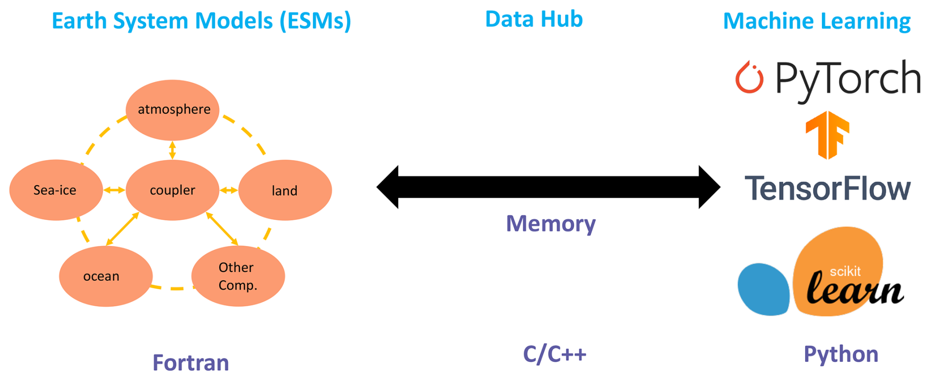
Figure 1 The interface of the ML bridge for two-way communication via memory between the Fortran ESM and the Python ML module.

In this study, we investigate the integration of ML parameterizations into Fortran-based ESM models by establishing a flexible interface that enables the invocation of ML algorithms in Python from Fortran. This integration offers access to any Python codes from Fortran, including a diverse range of ML frameworks, such as PyTorch, TensorFlow, and scikit-learn, which can effectively be utilized for parameterizing intricate atmospheric and other climate system processes. The coupling of the Fortran model and the Python ML code needs to be performed for thousands of model columns and over thousands of time steps for a typical model simulation. Therefore, it is crucial for the coupling interface to be both robust and efficient. We showcase the feasibility and benefits of this approach through case studies that involve the parameterization of deep convection and wildfire processes in ESMs. The two cases demonstrate the robustness and efficiency of the coupling interface. The focus of this paper is on documenting the coupling between the Fortran ESM and the ML algorithms and systematically evaluating the computational efficiency and memory usage of different ML frameworks (such as PyTorch and TensorFlow), different ML algorithms, and different configuration of a climate model. The assessment of the scientific performance of the ML emulators will be addressed in follow-on papers. The showcase examples emphasize the potential for high modularity and reusability by separating the ML components into Python modules. This modular design facilitates independent development and testing of ML-based parameterizations by researchers. It enables easier code maintenance, updates, and the adoption of state-of-the-art ML techniques with only minimal disruption to the existing Fortran infrastructure. Ultimately, this advancement will contribute to enhanced predictions and a deeper comprehension of the evolving climate of our planet. It is important to note that the current interface only supports executing deep learning algorithms on CPUs and does not support running them on GPUs.

The rest of this paper is organized as follows: Sect. 2 presents the detailed interface that integrates ML into Fortran-based ESM models. Section 3 discusses the performance of the interface and presents its application in two case studies. Finally, Sect. 4 provides a summary of the findings and a discussion of their implications.

2 General design of the ML interface

2.1 Architecture of the ML interface

We developed an interface using shared memory to enable two-way coupling between Fortran and Python (Fig. 1). The ESM used in the demonstration in Fig. 1 is the U.S. Department of Energy (DOE) Energy Exascale Earth System Model (E3SM; Golaz et al., 2019, 2022). Because Fortran cannot directly call Python, we utilized C as an intermediary since Fortran can call C functions. This approach leverages C as a data hub to exchange information without requiring a framework-specific binding like KFB. As a result, our interface supports invoking any Python-based ML package such as PyTorch, TensorFlow, and scikit-learn from Fortran. While C can access Python scalar values through the built-in PyObject_CallObject function from the Python C API, we employed Cython for its ability to transfer array data between the languages. Using Cython, multidimensional data structures can be efficiently passed between Fortran and Python modules via C, allowing for flexible training of ML algorithms within ESMs.

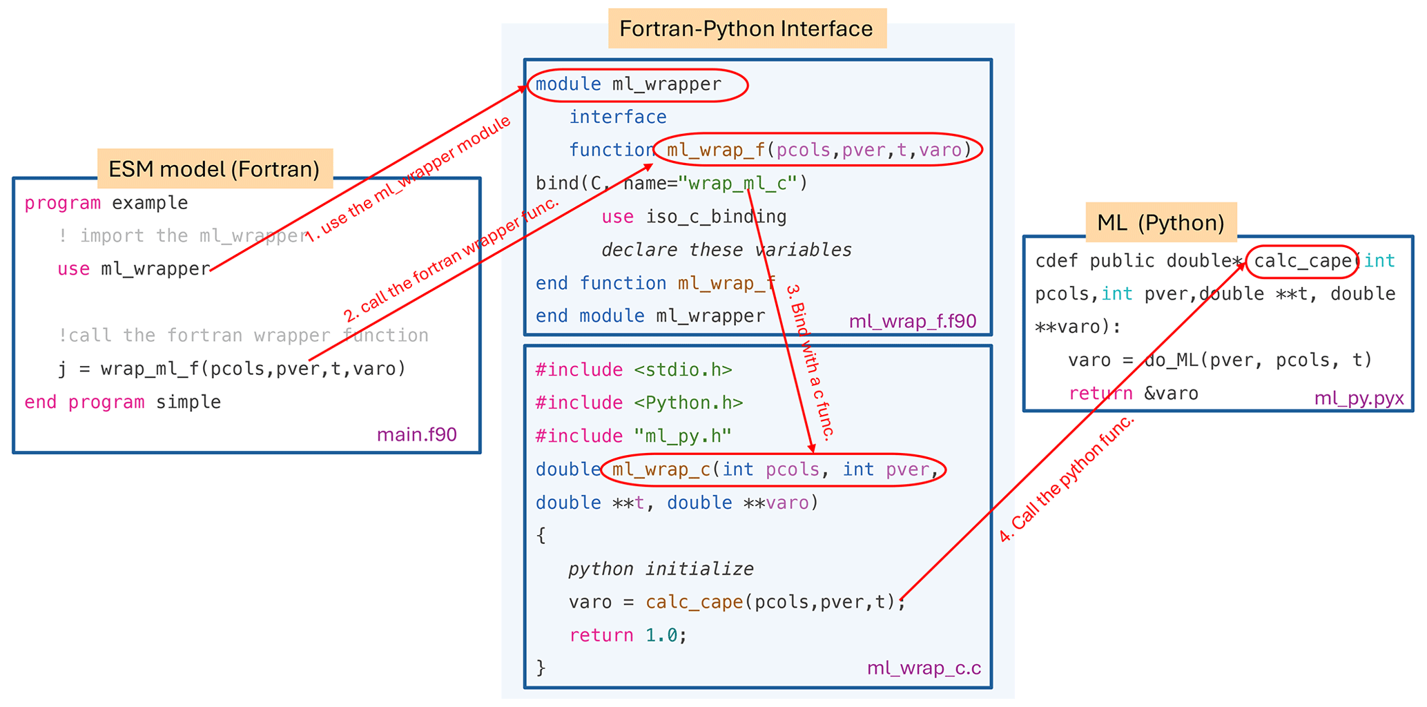
Figure 2 Toy code illustrating the Fortran–Python interface. It is noted that a fleshed-out, compliable version of this toy example exists in the linked GitHub repository.

2.2 Code structure

Figure 2 illustrates how the framework operates using a toy code example. The Fortran–Python interface comprises a Fortran wrapper and C wrapper files, which are bound together. The Fortran-based ESM first imports the Fortran wrapper, allowing it to call wrapper functions with input and output memory addresses. The interface then passes these memory addresses to the Python-based ML module, which performs the ML predictions and returns the output address to the Fortran model.

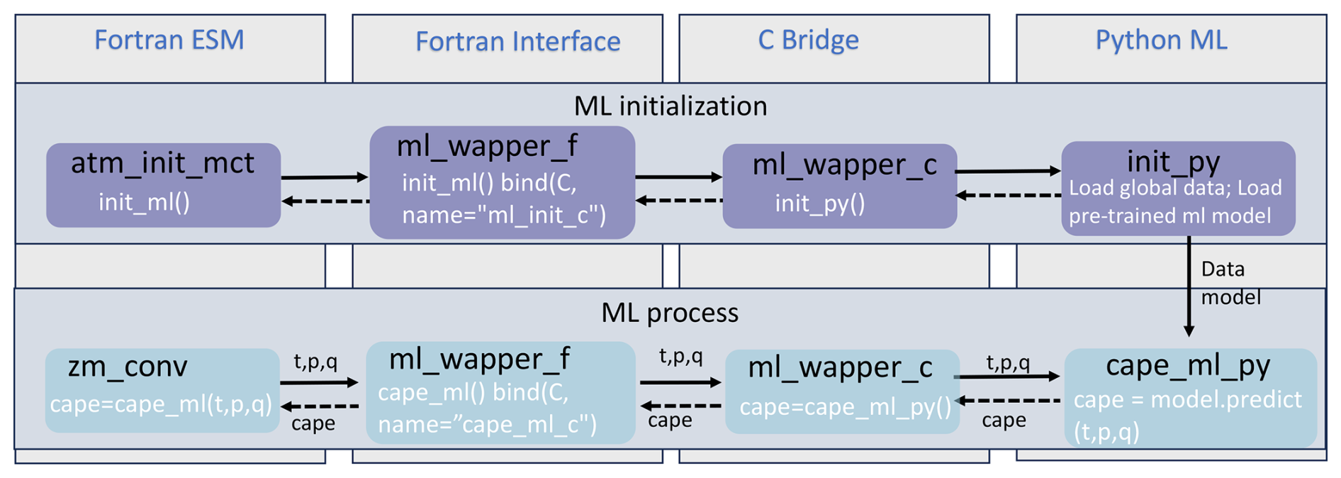
Figure 3 The code structure of the ML bridge interface using the ML closure in deep convection as an example.

When coupling the Python ML module with the Fortran model using the interface, additional steps should be considered: (1) the ML module should remain active throughout the model simulations, without any Python finalization calls, ensuring it is continuously available. (2) The Python module should load the trained ML model and any required global data only once rather than at each simulation step. This one-time initialization process improves efficiency and prevents unnecessary repetition. On the Fortran ESM side, the init_ml() function is called within the atm_init_mct module to load the ML model and global data (shown in Fig. 3). Then, similar to the toy code, we call the wrapper function, pass input variables to Python for ML predictions, and return the results to the Fortran side. (3) When compiling the complex system, which includes Python, C, Cython, and Fortran code, the Python path should be specified in the CFLAGS and LDFLAGS. It is important to note that without the position-independent compiling flag (-fPIC), the hybrid system will only work on a single node and may cause segmentation faults on multiple nodes. Including it can resolve this issue, allowing multi-node compatibility.

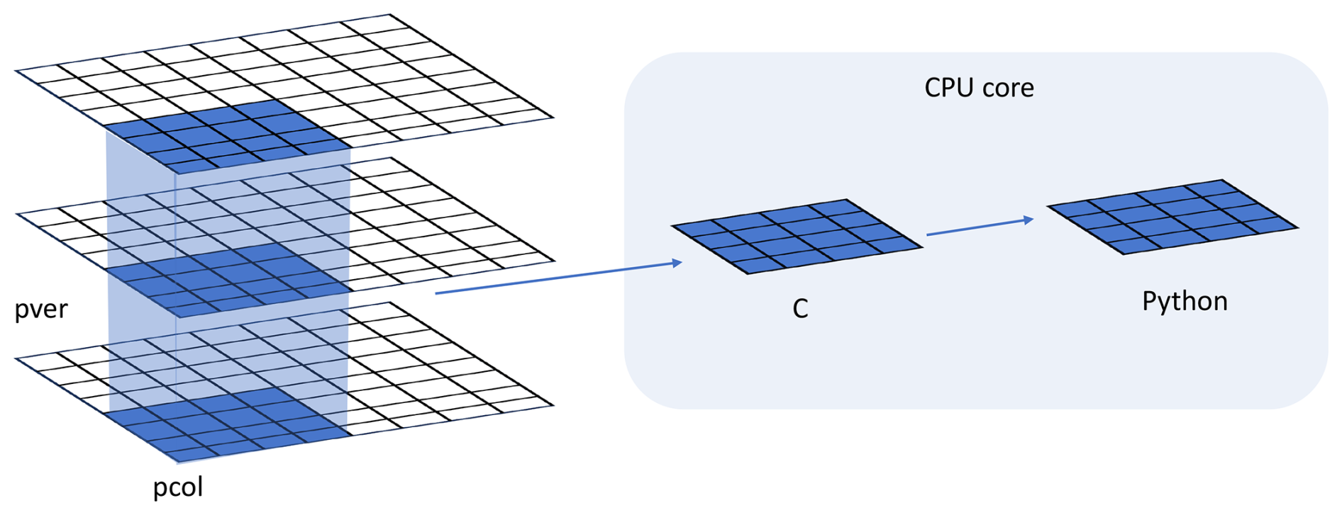
Figure 4 Data and system structure. The model domain is decomposed into chunks of columns. pver refers to number of pressure vertical levels. A chunk contains multiple columns (up to pcol). Multiple chunks can be assigned to each CPU core.

In traditional ESMs, subgrid-scale parameterization routines such as convection parameterizations are often calculated separately for each vertical column of the model domain. Meanwhile, the domain is typically decomposed horizontally into 2D chunks that can be solved in parallel using MPI processes. Each CPU core/MPI process is assigned a number of chunks of model columns to update asynchronously (Fig. 4). Our interface takes advantage of this existing parallel decomposition by designing the ML calls to operate over all columns simultaneously within each chunk rather than invoking the ML scheme individually for each column. This allows the coupled model–ML system to leverage parallelism in the neural network computations. If the ML were called separately for every column, parallel efficiencies would not be realized. By aggregating inputs over the chunk-scale prior to interfacing with Python, performance is improved through better utilization of multi-core and GPU-based ML capabilities during parameterization calculations.

3 Results

The framework explained in the previous section provides seamless support for various ML parameterizations and various ML frameworks, such as PyTorch, TensorFlow, and scikit-learn. To demonstrate the versatility of this framework, we applied it in two distinct case applications. The first application replaces the conventional CAPE-based trigger function in a deep convection parameterization with a machine-learned trigger function. The second application involves an ML-based wildfire model that interacts bidirectionally with the ESM. We provide a brief introduction to these two cases. Detailed descriptions and evaluations will be presented in separate papers.

The framework's performance is influenced by two primary factors: increasing memory usage and increasing computational overhead. Firstly, maintaining the Python environment fully persistent in memory throughout model simulations can impact memory usage, especially for large ML algorithms. This elevated memory footprint increases the risk of leaks or crashes as simulations progress. Secondly, executing ML components within the Python interpreter inevitably introduces some overhead compared to the original ESMs. The increased memory requirements and decreased computational efficiency associated with these considerations can impact the framework's usability, flexibility, and scalability for different applications.

To comprehensively assess performance, we conducted a systematic evaluation of various ML frameworks, ML algorithms, and physical models. This evaluation is built upon the foundations established for evaluating the ML trigger function in the deep convection parameterization.

3.1 Application cases

3.1.1 ML trigger function in deep convection parameterization

In general circulation models, uncertainties in convection parameterizations are recognized to be closely linked to the convection trigger function used in these schemes (Bechtold et al., 2004; Lee et al., 2007; Xie et al., 2004; Xie and Zhang, 2000). The convective trigger in a convective parameterization determines when and where model convection should be triggered as the simulation advances. In many convection parameterizations, the trigger function consists of a simple, arbitrary threshold for a physical quantity, such as convective available potential energy (CAPE). Convection will be triggered if the CAPE value exceeds a threshold value.

In this work, we use this interface to test a newly developed ML trigger function in E3SM. The ML trigger function was developed with the training data originating from simulations performed using the kilometer-resolution (1.5 km grid spacing) Met Office Unified Model Regional Atmosphere 1.0 configuration (Bush et al., 2020). Each simulation consists of a limited area model (LAM) nested within a global forecast model providing boundary conditions (Walters et al., 2017; Webster et al., 2008). In total 80 LAM simulations were run located so as to sample different geographical regions worldwide. Each LAM was run for 1 month, with 2-hourly output, using a grid length of 1.5 km, a 512 × domain, and a model physics package used for operational weather forecasting. The 1.5 km data are coarse-grained to several scales from 15 to 144 km.

A two-stream neural network architecture is used for the ML model. The first stream takes profiles of temperature, specific humidity, and pressure across 72 levels at each scale as inputs and passes them through a 4-layer convolutional neural network (CNN) with kernel sizes of 3 to extract large-scale features. The second stream takes mean orographic height, standard deviation of orographic height, land fraction, and the size of the grid box as inputs. The outputs of the two streams are then combined and fed into a two-layer fully connected network to allow the ML model to leverage both atmospheric and surface features when making its predictions. The output is a binary variable indicating whether the convection happens, based on the condition of buoyant cloudy updrafts (BCUs; e.g., Hartmann et al., 2019; Swann, 2001). If there are three contiguous levels where the predicted BCU is larger than 0.05, the convection scheme is triggered. Once trained, the CNN is coupled to E3SM, and thermodynamic information from E3SM is passed to it to predict the trigger condition. Then, the predicted result is returned to E3SM.

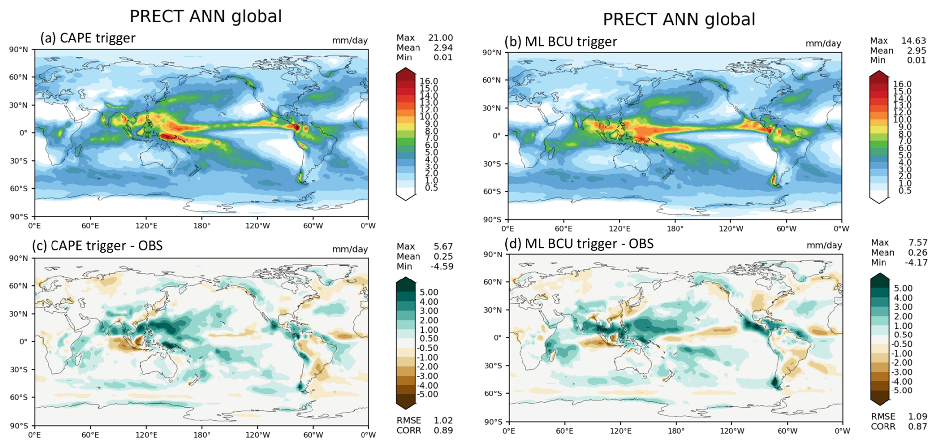
Figure 5 Comparison of annual mean precipitation between the control run using the CAPE-based trigger function (a, c) and the run using the ML BCU trigger function (b, d).

Figure 5 shows the comparison of annual mean precipitation between the control run using the traditional CAPE-based trigger function and the run using the ML BCU trigger function. The ML BCU scheme demonstrates reasonable spatial patterns of precipitation, similar to the control run, with comparable root-mean-square error and spatial correlation. Additional experiments exploring the definition of BCU and varying the thresholds along with an in-depth analysis will be presented in a follow-up paper.

3.1.2 ML learning fire model

Predicting wildfire burned area is challenging due to the complex interrelationships between fires, climate, weather, vegetation, topography, and human activities (Huang et al., 2020). Traditionally, statistical methods like multiple linear regression have been applied but are limited in the number and diversity of predictors considered (Yue et al., 2013). In this study, we develop a coupled fire–land–atmosphere framework that uses machine learning to predict wildfire area, enhancing long-term burned area projections and assessing fire impacts by enabling simulations of interactions among fire, atmosphere, land cover, and vegetation.

The ML algorithm is trained using a monthly dataset, which includes the target variable of burned area, as well as various predictor variables. These predictors encompass local meteorological data (e.g., surface temperature, precipitation), land surface properties (e.g., monthly mean evapotranspiration and surface soil moisture), and socioeconomic variables (e.g., gross domestic product, population density), as described by Wang et al. (2022a). In the coupled fire–land–atmosphere framework, meteorology variables and land surface properties are provided by the E3SM. We use the eXtreme Gradient Boosting (XGBoost) algorithm implemented in scikit-learn to train the ML fire model. Figure 6 demonstrates that the ML4Fire model exhibits superior performance in terms of spatial distribution compared to process-based fire models, particularly in the southern US region. Detailed analysis will be presented in a separate paper. The ML4Fire model has proven to be a valuable tool for studying vegetation–fire interactions, enabling seamless exploration of climate–fire feedbacks.

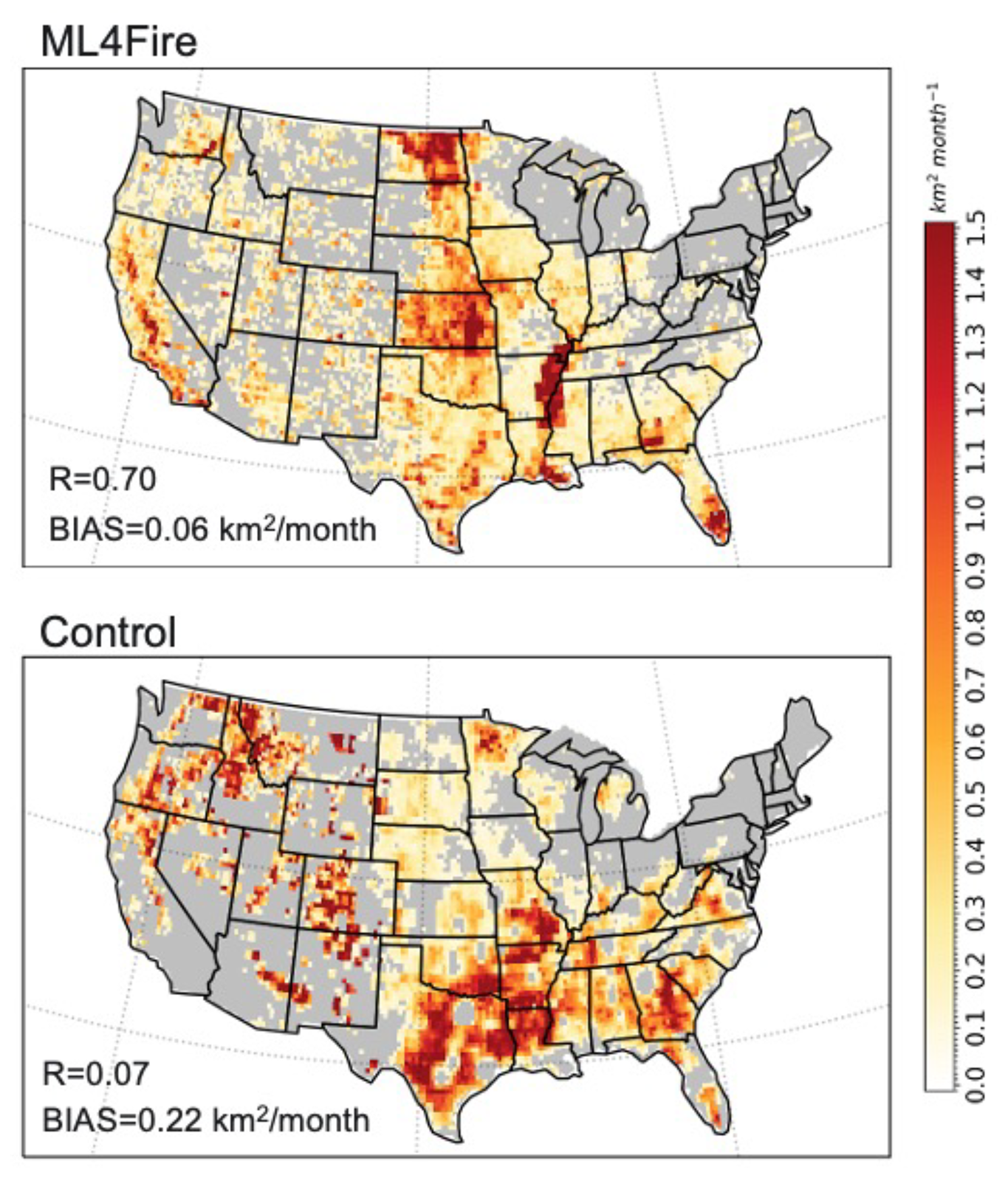
Figure 6 Comparison between the ML4Fire model and the process-based fire model against the historical burned area from Global Fire Emissions Database 5 from 2001–2020. R and BIAS are the spatial pattern correlation and difference against the observation, respectively.

3.2 Performance of different ML frameworks

The Fortran–Python bridge ML interface supports various ML frameworks, including PyTorch, TensorFlow, and scikit-learn. These ML frameworks can be trained offline using kilometer-scale high-resolution models (such as the ML trigger function) or observations (ML fire model). Once trained, they can be plugged into the ML bridge interface through different API interfaces specific to each framework. The coupled ML algorithms are persistently resident in memory, just like the other ESM components. During each step of the process, the performance of the full system is significantly affected by memory usage. If memory consumption increases substantially, it may lead to memory leaks as the number of time step iterations increases. In addition, Python, being an interpreted language, is typically considered to have slower performance compared to compiled languages like C/C++ and Fortran. Therefore, incorporating Python may decrease computational performance. We examine the memory usage and computational performance across various ML frameworks based on implementing the ML trigger function in E3SM. The ML algorithm is implemented as a two-stream CNN model using Pytorch and TensorFlow frameworks, as well as XGBoost using the scikit-learn package. It should be noted that XGBoost, a boosting tree-based model, is a completely different type of ML model compared to the CNNs, whose type is deep neural network.

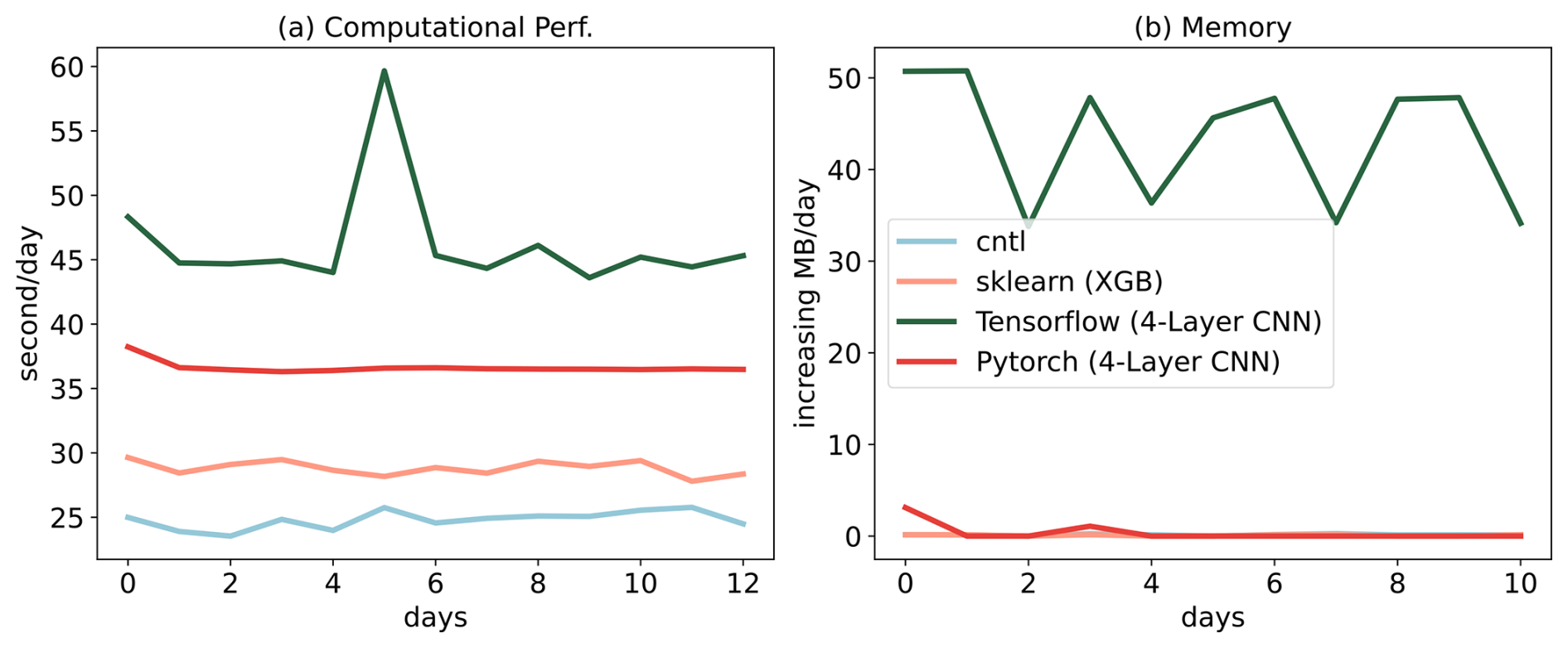
Figure 7 Computational and memory overhead as the simulation progresses for coupling the ML trigger function with the E3SM model. The x axis represents the simulated time step. The y axis of (a) represents the simulation speed measured in seconds per day (indicating the number of seconds required to simulate one day). The y axis of (b) represents the relative increase in memory usage for scikit-learn, TensorFlow, and PyTorch compared with CNTL. CNTL represents the original simulation without using the ML framework.

Figure 7 illustrates the computational and memory overhead associated with the ML parameterization using different ML frameworks. It shows that XGBoost only exhibits a 20 % increase in the simulation time required for simulating 1 d due to its simpler algorithm. For more complex neural networks, PyTorch incurs a 52 % overhead, while TensorFlow's overhead is almost 100 % – about 2 times as much as the overhead of PyTorch. In terms of memory usage, we use the high-water memory metric (Gerber, 2013), which represents the total memory footprint of a process. PyTorch and scikit-learn do not show any significant increase in memory usage. However, TensorFlow shows a considerable increase up to 50 MB per simulation day per MPI process element. This is significant because for a node with 48 cores, it would equate to an increase of around 2 GB per simulated day on that node. This rapid memory growth could quickly lead to a simulation crash due to insufficient memory during continuous integrations, preventing the use in practical simulations. Our findings show that the TensorFlow prediction function does not release memory after each call. Therefore, we recommend using PyTorch for complex deep learning algorithms and scikit-learn for simpler ML algorithms to avoid these potential memory-related issues when using TensorFlow. Previous work, such as Brenowitz and Bretherton (2018, 2019), has utilized the CFFI package to establish communication between Fortran ESM and ML Python. As described in the Introduction, while CFFI offers flexibility in supporting various ML packages, it does have certain limitations. To pass variables from Fortran to Python, the approach relies on global data structures to store all variables, including both the input from Fortran to Python and the output returning to Fortran. Consequently, this package results in additional memory copy operations and increasing overall memory usage. In contrast, our interface takes a different approach by utilizing memory references to transfer data between Fortran and Python, avoiding the need for global data structures and the associated overhead. This allows for a more efficient data transfer process.

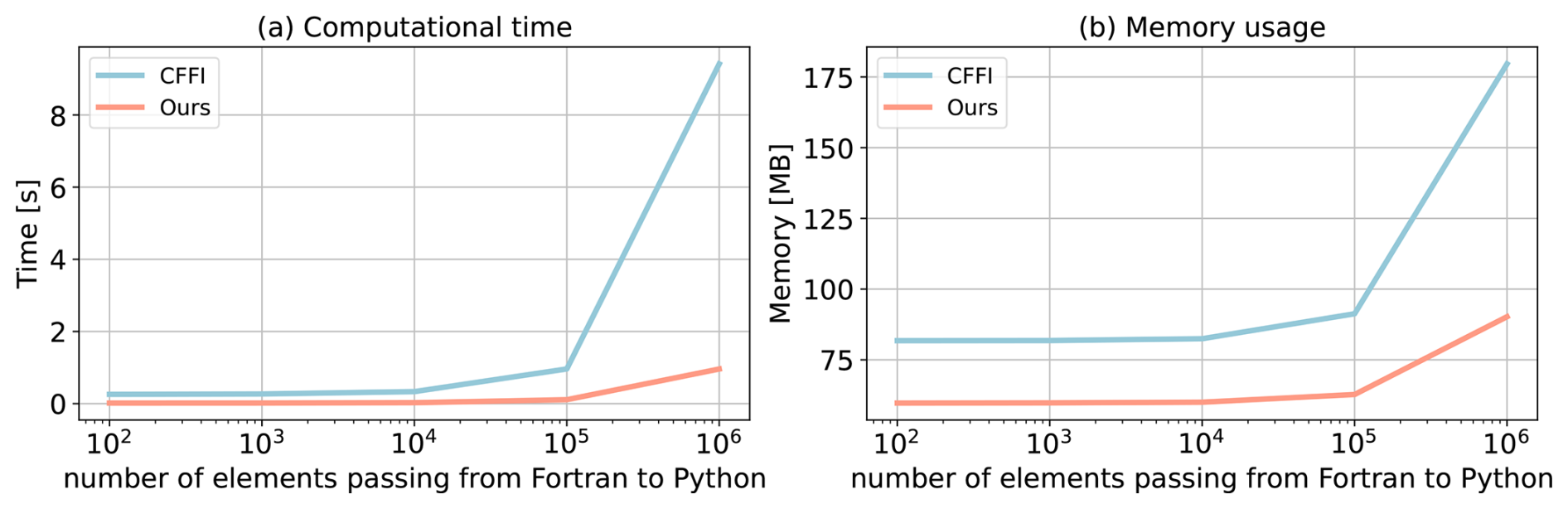
Figure 8 Comparison of our framework and the CFFI framework in terms of computational time and memory usage. The x axis represents the number of elements transferred from Fortran to Python, while the y axis displays the total time (a) and total memory usage (b) for a demonstration example. The evaluations presented are based on the average results obtained from five separate tests.

In Fig. 8, we present a comparison between the two frameworks by testing the different number of elements passed from Fortran to Python. The evaluation is based on a demo example that focuses solely on declaring arrays and transferring them from Fortran to Python rather than a real E3SM simulation. Figure 8a illustrates the impact of the number of passing elements on the overhead of the two interfaces. As the number of elements exceeds 10⁴, the overhead of CFFI becomes significant. When the number surpasses 10⁶, the overhead of CFFI is nearly 10 times greater than that of our interface. Regarding memory usage, our interface maintains a stable memory footprint of approximately 60 MB. Even as the number of elements increases, the memory usage only shows minimal growth. However, for CFFI, the memory usage starts at 80 MB, which is 33 % higher than our interface. As the number of elements reaches 10⁶, the memory overhead for CFFI dramatically rises to 180 MB, twice as much as our interface.

3.3 Performance of ML algorithms of different complexities

ML parameterizations can be implemented using various deep learning algorithms with different levels of complexity. The computational performance and memory usage can be influenced by the complexity of these algorithms. In the case of the ML trigger function, a two-stream four-layer CNN structure is employed. We compare this structure with other ML algorithms such as artificial neural network (ANN) and residual network (ResNet), whose structures are detailed in Table 1. We selected these three ML algorithms because they have commonly been used in previous ML parameterization approaches, such as Brenowitz and Bretherton (2019), Han et al. (2020), and Wang et al. (2022b). Systematically evaluating the hybrid system with these ML methods using our interface can help identify bottlenecks and improve the system computational performance. These algorithms are implemented in PyTorch. The algorithm's complexity is measured by the number of parameters, with the CNN having approximately 60 times more parameters than ANN and ResNet having roughly 1.5 times more parameters than CNN.

Table 1 The structure and number of parameters of each ML algorithm. Linear is a fully connected layer that applies a linear transformation to the input. Conv2d is a 2D convolution layer in PyTorch.

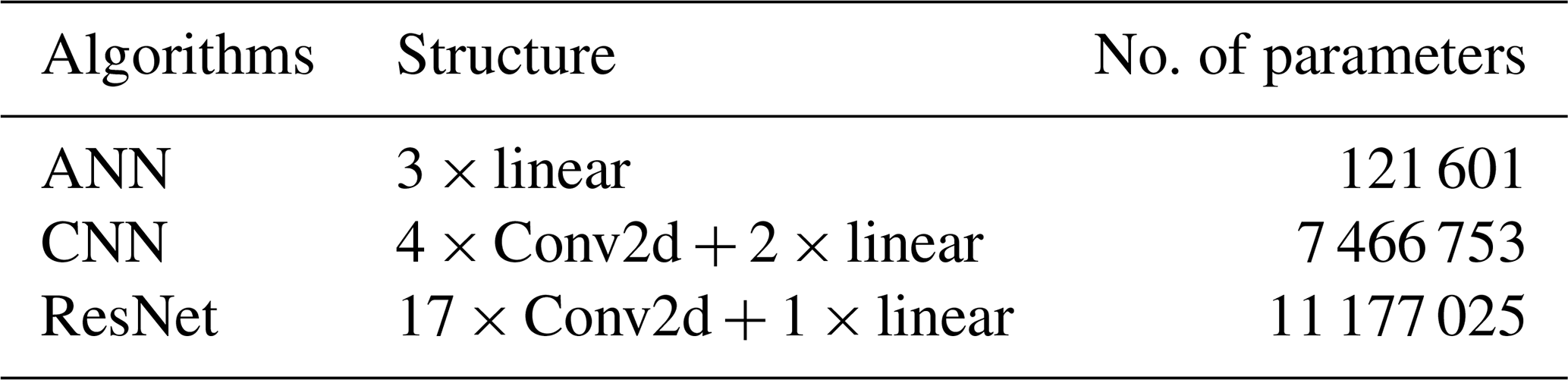
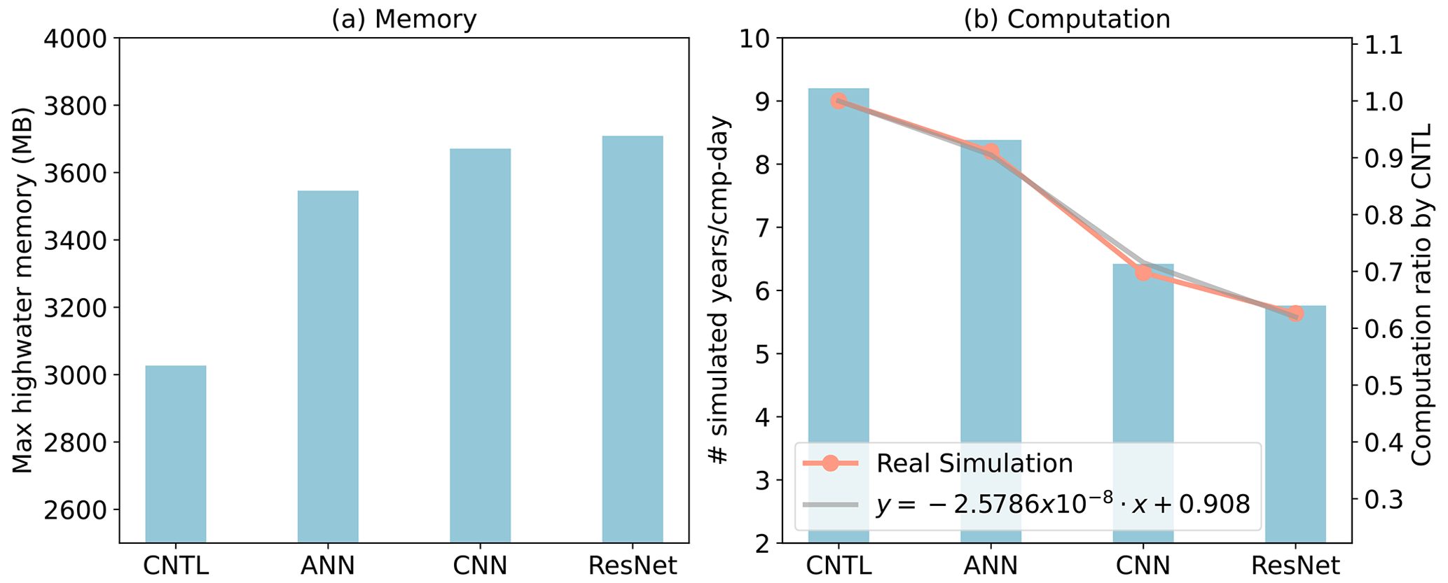
Figure 9 Comparison of CNTL and the hybrid model using various ML algorithms in terms of memory and computation. CNTL is the default run without ML parameterizations. In (b), the left y axis represents the actual number of simulated years per day, while the right y axis shows the relative performance compared to the CNTL run (orange line). The gray line illustrates the regression between the number of ML parameters (x) and the relative performance of the hybrid system (y).

Figure 9 presents a comparison of the memory and computational costs between the CNTL run without deep learning parameterization and the hybrid run with various deep learning algorithms. The same specific process–element layout (placement of ESM component models on distributed CPU cores) is used for all the simulations. Deep learning algorithms incur a significant yet affordable increase in memory overhead, with at least a 20 % increase compared to the CNTL run (Fig. 9a). This is primarily due to the integration of ML algorithms into the ESM, which persists throughout the simulations. Although there is a notable increase in complexity among the deep learning algorithms, their memory usage only shows a slight rise. This is because the memory increment resulting from the ML parameters is relatively small. Specifically, the ANN algorithm requires 1 MB of memory, CNN requires 60 MB, and ResNet requires 85 MB, which are calculated based on the number of parameters in each algorithm. When comparing these values to the memory consumption of the CNTL run, which is approximately 3000 MB, the additional parameters' incremental memory consumption is not substantial. However, when we use 128 MPI processes per node, it could bring the total memory requirement to approximately 460 GB per node. If the available hardware memory is less than this, the process layout must be adjusted accordingly.

In terms of computational performance, the Python-based ML calls inevitably introduce some overhead. However, as shown in Fig. 9b, the performance decrease is not substantial. The simple ANN model reduces performance by only about 10 % compared to the CNTL run, while even the more complex ResNet model results in a 35 % decrease. In contrast, Wang et al. (2022b) reported a 100 % overhead in their interface when using the ResNet model as well, which transfers parameters via files. It is worth noting that in this study, the deep learning algorithms are executed on CPUs. To enhance computational performance, future work could consider utilizing GPUs for acceleration.

In addition, we develop a performance model to estimate computational performance for the hybrid model using different ML model sizes and complexities. This performance model, based on linear regression, predicts the ratio of the simulated years per day of the ML-augmented run to that of the CNTL run as a function of the number of ML parameters, shown in Fig. 9b. It provides a simple yet effective way to capture this relationship and serves as a valuable tool for performance prediction when incorporating more complicated ML models.

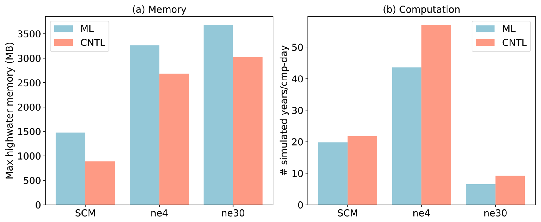
Figure 10 Comparison of CNTL and ML for various ESMs in terms of memory and computation. The ESM configuration includes SCM, ultra-low-resolution model (ne4), and nominal low-resolution model (ne30).

3.4 Performance for physical models of different complexities

ML parameterization can be applied to various ESM configurations. In the E3SM Atmosphere Model (EAM), we experiment with configurations involving a single-column model (SCM), the ultra-low-resolution model of EAM (ne4), and the nominal low-resolution model of EAM (ne30). The SCM consists of one single atmosphere column of a global EAM (Bogenschutz et al., 2020; Gettelman et al., 2019). ne4 has 384 columns, with each column representing the horizontal resolution of 7.5°. ne30 is the default resolution for EAM and comprises 21 600 columns, with each column representing the horizontal resolution of 1°. In the case of the ML trigger function, the memory overhead is approximately 500 MB for all configurations due to the loading of the ML algorithm, which does not vary with the configuration of the ESM.

Regarding computational performance, SCM utilizes 1 process, ne4 employs 1 node with 64 processes, and ne30 utilizes 10 nodes with each node using 128 processes. In the case of SCM, the overhead attributed to the ML parameterization is approximately 9 % due to the utilization of only one process. However, for ne4 and ne30, the overhead is 23 % and 28 %, respectively (Fig. 10). The increasing computational overhead is primarily due to resource competition when multiple processes are used within a single node. It is noted that although there is a significant computational gap between ML and CNTL for ne4, the relative performance between ML and CNTL for ne4 is approximately 76.7 %, which is close to ne30 at 71.4 %.

4 Discussion and conclusion

ML algorithms can learn detailed information about cloud processes and atmospheric dynamics from kilometer-scale models and observations and serves as an approximate surrogate for the kilometer-scale model. Instead of explicitly simulating kilometer-scale processes, the ML algorithms can be designed to capture the essential features and relationships between atmospheric variables by training on available kilometer-scale data. The trained algorithms can then be used to develop parameterizations for use in models at coarser resolutions, reducing the computational and memory costs. By using ML parameterizations, scientists can effectively incorporate the insights gained from kilometer-scale models for coarser-resolution simulations. Through learning the complex relationships and patterns present in the high-resolution data, the ML-based parameterizations have the potentials to more accurately represent cloud processes and atmospheric dynamics in the ESMs. This approach strikes a balance between computational efficiency and capturing critical processes, enabling more realistic simulations and predictions while minimizing computational resources. All these potential benefits in turn promote innovative developments to facilitate increasing and more efficient use of ML parameterizations. In this study, we develop a novel Fortran–Python interface for developing ML parameterizations. This interface demonstrates feasibility in supporting various ML frameworks, such as PyTorch, TensorFlow, and scikit-learn, and enables the effective development of new ML-based parameterizations to explore ML-based applications in ESMs. Through two cases – an ML trigger function in convection parameterization and an ML wildfire model – we highlight high modularity and reusability of the framework. We conduct a systematic evaluation of memory usage and computational overhead from the integrated Python codes.

Based on our performance evaluation, we observe that coupling ML algorithms using TensorFlow into ESMs can lead to memory leaks. As a recommendation, we suggest using PyTorch for complex deep learning algorithms and scikit-learn for simple ML algorithms for the Fortran–Python ML interface.

The memory overhead primarily arises from loading ML algorithms into ESMs. If the ML algorithms are implemented using PyTorch or scikit-learn, the memory usage will not increase significantly. The computational overhead is influenced by the complexity of the neural network and the number of processes running on a single node. As the complexity of the neural network increases, more parameters in the neural network require forward computation. Similarly, when there are more processes running on a single node, the integrated Python codes introduce more resource competition.

Although this interface provides a flexible tool for ML parameterizations, it does not currently utilize GPUs for ML algorithms. In Fig. 3, it is shown that each chunk is assigned to a CPU core. However, to effectively leverage GPUs, it is necessary to gather the variables from multiple chunks and pass them to the GPUs. Additionally, if an ESM calls the Python ML module multiple times in each time step, the computational overhead becomes significant. It is crucial to gather the variables and minimize the number of calls. In the future, we will enhance the framework to support this mechanism, enabling GPU utilization and overall performance improvement.