Towards deep-learning solutions for classification of automated snow height measurements (CleanSnow v1.0.2)

Snow height measurements are still the backbone of any snow cover monitoring, whether based on modeling or remote sensing. These ground-based measurements are often realized using ultrasonic or laser technologies. In challenging environments, such as high alpine regions, the quality of sensor measurements deteriorates quickly, especially under extreme weather conditions or ephemeral snow conditions. Moreover, the sensors by their nature measure the height of an underlying object and are therefore prone to returning other information, such as the height of vegetation, in snow-free periods. Quality assessment and real-time classification of automated snow height measurements are therefore desirable for providing high-quality data for research and operational applications. To this end, we propose CleanSnow, a machine learning approach to automated classification of snow height measurements into a snow cover class and a class corresponding to everything else, which takes into account both the temporal context and the dependencies between snow height and other sensor measurements. We created a new dataset of manually annotated snow height measurements, which allowed us to train our models in a supervised manner and quantitatively evaluate our results. Through a series of experiments and ablation studies to evaluate feature importance and compare several different models, we validated our design choices and demonstrated the importance of using temporal information together with information from auxiliary sensors. CleanSnow achieves a high accuracy of almost 98 % and represents a new baseline for further research in the field. The presented approach to snow height classification finds its use in various tasks, ranging from snow modeling to climate science.

1 Introduction

Snow height measurements are key in many fields, such as water resource management, avalanche forecasting, climate science, and even tourism. A variety of complex models simulating and calculating snowpack properties therefore exist. For example, they estimate snow water equivalent (SWE) (e.g., Jonas et al., 2009) in order to assess water resources. In addition, snow height is an important parameter for snow hydrological (e.g., Mott et al., 2023) and snow cover (Lehning et al., 1999) modeling used in operational avalanche forecasting (Morin et al., 2020; Pérez-Guillén et al., 2022; Herla et al., 2024). In climate science, snow cover is one of the key variables that strongly affect the global energy balance and the atmospheric circulation, due to its high albedo, high emissivity, and low thermal conductivity (e.g., Flanner et al., 2011). Snow height signals have also been used to determine vegetation growth and plant phenology (e.g., Jonas et al., 2008; Fontana et al., 2008; Vitasse et al., 2017) and to monitor climate change (e.g., Matiu et al., 2021). Finally, the snow cover directly influences tourism, transportation, and recreational activities (e.g., Willibald et al., 2021).

Snow height data are available nowadays, sometimes in near real time, from airborne or satellite remote sensing and ground-based automated weather stations (AWSs). One of the sensors often mounted at meteorological stations in high alpine regions is an ultrasonic snow height sensor (Ryan et al., 2008). Due to the measurement method, snow height data come with a variety of errors that arise from the harsh mountain conditions that the sensor is not originally designed to operate under. In addition, ultrasonic sensors only measure the distance to the underlying object, be it snow or anything else. It is therefore important to validate whether the information coming from the snow height sensor really corresponds to snow or not.

Arguably the most precise way of assessing the quality of snow height measurements is via visual inspection of the data by a human expert (Robinson, 1989), which is however not easily transferable and does not scale well (Fiebrich et al., 2010). A common practice in both manual and automated snow height quality assessment is to distinguish between snow and grass based on static climatological or minimum snow height thresholds. Random errors are typically detected using a maximum snow height threshold or snow height variance (Avanzi et al., 2014).

There are other sensors usually mounted at an AWS, whose temporal structure can provide information on whether the measured snow height relates to snow or not and give some indications of the precision of snow height measurement. Fusion of temporal information from multiple sensors results in high-dimensional multivariate time series signals, which increases the complexity of the problem. The first attempts to leverage other sensor information included the MeteoIO library developed by Bavay and Egger (2014) and the thresholding method of Tilg et al. (2015). Both algorithms are based on a series of thresholding rules that follow the physical properties of snow. In particular, with the presence of snow, the snow surface temperature (TSS) is expected to be ≤0 °C. The ground temperature (TG) is expected to be constantly around 0 °C, as snow insulates the ground from atmospheric temperature variations (Domine, 2011). Reflected shortwave radiation (RSWR) is expected to be high since snow has a much higher albedo than soil or vegetation. When no snow is present, both TSS and TG typically show diurnal variations, in line with the air temperature (TA). However, it is rather difficult to capture correlations between different features in high-dimensional space by defining thresholding rules. Moreover, thresholding approaches are known to be rather cumbersome to modify and generally do not transfer well to other station data.

Machine learning, instead, is an appropriate choice in such cases and has already shown its power in other tasks concerning weather and climate data (e.g., Vaughan et al., 2022; Luković et al., 2022; Lam et al., 2023). Blandini et al. (2023) addressed the high dimensionality of the data with a random forest (RF) approach to snow height quality assessment, solving both snow height classification and anomaly detection at the same time. RF models (Breiman, 2001) are amongst the most popular choices of machine learning algorithms for tabular data (Grinsztajn et al., 2022). Multivariate time series signals contain both temporal dependencies between different data points from the same sensor and inter-sensor correlations between measurements from multiple different sensors. Apart from an attempt by Goehry et al. (2023), simple models such as random forests or multilayer perceptron (MLP) neural networks (Rosenblatt, 1958; Hornik et al., 1989; Cybenko, 1989) cannot explicitly account for the temporal nature of the data without engineering complex and artificial features, and therefore they are a rather poor design choice. To correctly capture temporal patterns in the data, we instead choose to work with neural network models specifically designed to operate on time series data, e.g., recurrent neural networks (RNNs) (McCulloch and Pitts, 1943; Kleene, 1951), long short-term memory (LSTM) networks (Hochreiter and Schmidhuber, 1997), temporal convolutional networks (TCNs) (Lea et al., 2016), TimesNet (Wu et al., 2023), or transformers (Vaswani et al., 2017).

We developed CleanSnow, a machine learning model for automated classification of snow height signals into the Snow and No Snow classes. To approach this binary classification problem, we employed a temporal convolutional network that explicitly accounts for the temporal relationships between different points in snow height time series data. To train our TCN, we created a new manually annotated snow height dataset composed of 20 measurement stations with around 20 years of data per station. This dataset also allows us to validate our design choices and evaluate the model in several different scenarios, including challenging cases such as snow cover melt or plant growth periods.

2 Data

We used snow height data from the Swiss Intercantonal Measurement and Information System (IMIS) (Lehning et al., 1999; Liechti and Schweizer, 2024), a network of 131 AWSs (as of May 2024) focused on snow measurements that are distributed throughout the Swiss Alps and Jura (see Fig. 1) and are mostly located above 2000 $\mathrm{m}\mathrm{a}.\mathrm{s}.\mathrm{l}.$ The stations acquire data regularly in 30 min intervals and provide meteorological data in addition to snow height. To analyze snow height (HS), we also leverage measurements of TA, TSS, wind speed (WV), relative humidity (RH), and RSWR.

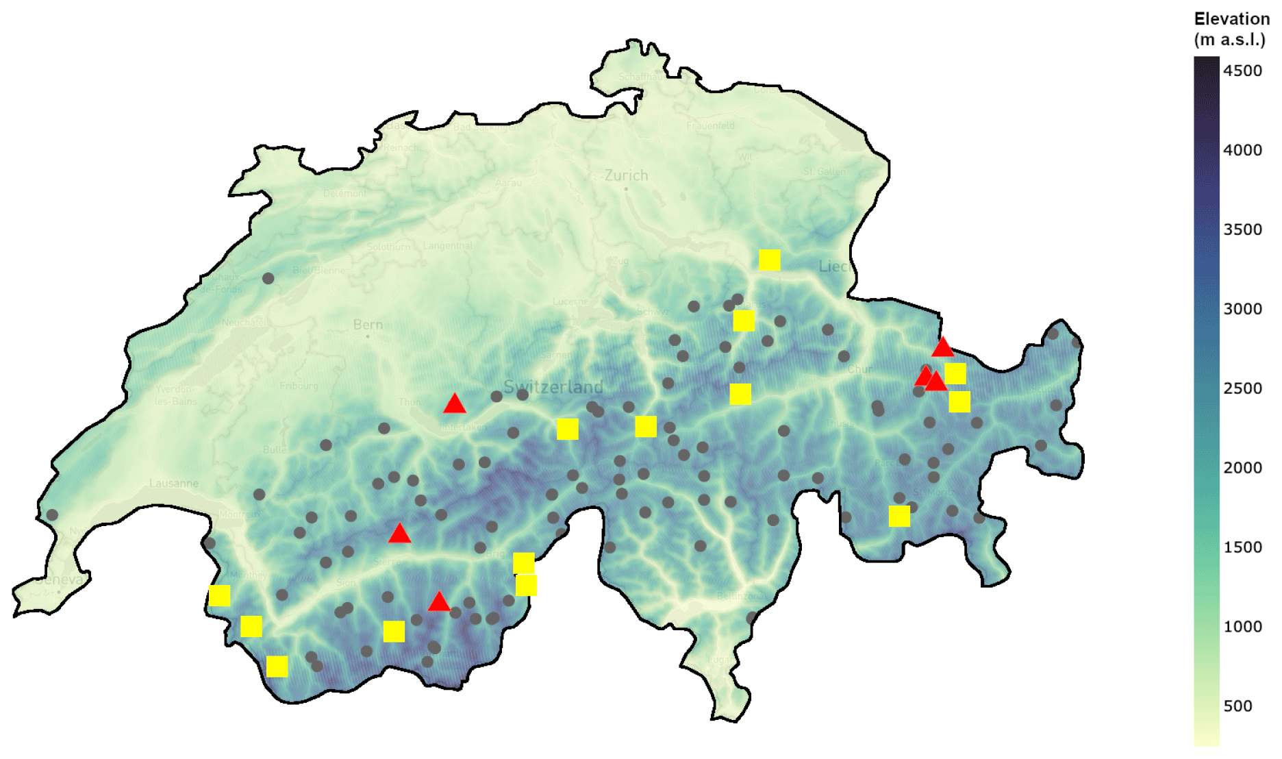
Figure 1 Map of IMIS stations in Switzerland. Stations marked as full gray circles were not part of the new annotated dataset. The yellow squares are the stations that were used for training (14 stations), and the red triangles indicate stations used for testing (6 stations). The background colors indicate the elevation ($\mathrm{m}\mathrm{a}.\mathrm{s}.\mathrm{l}.$).

2.1 Data preparation

For model development and validation, we prepared a dataset with reliable ground truth information. Manually annotating snow height data is a tedious process, and doing so for the whole IMIS network is intractable. Therefore, we identified a subset of IMIS stations that we then manually annotated.

Annotating historical data is rather difficult, as there is no way of checking whether there really was snow at a station or not. This means that assessing the presence of snow with the help of information from other sensors, such as TA, TSS, TG, and RSWR, should be considered a best-effort approach.

2.1.1 Snow or No Snow dataset

A subset of 20 stations (see Appendix A) which span different locations and elevations and vary in their underlying surfaces (e.g., vegetation, bare ground, and glacier) was selected and manually annotated with binary ground truth information regarding snow height data:

• Class 0 – No Snow: the surface is snow-free (e.g., vegetation, soil, and rocks).

• Class 1 – Snow: the surface is covered by snow.

The stations annotated with ground truth information are depicted in yellow and red in Fig. 1. An example of this data annotation is shown in Fig. 2, with two detailed views that emphasize the differences in the behavior of TSS and RSWR in the presence and absence of snow cover. The selected stations mostly contain data between 2000 and 2023 at a frequency of 30 min, with a few exceptions for stations that were built later (BOR2, FLU2, LAG3, RNZ2, and SHE2; see Appendix A).

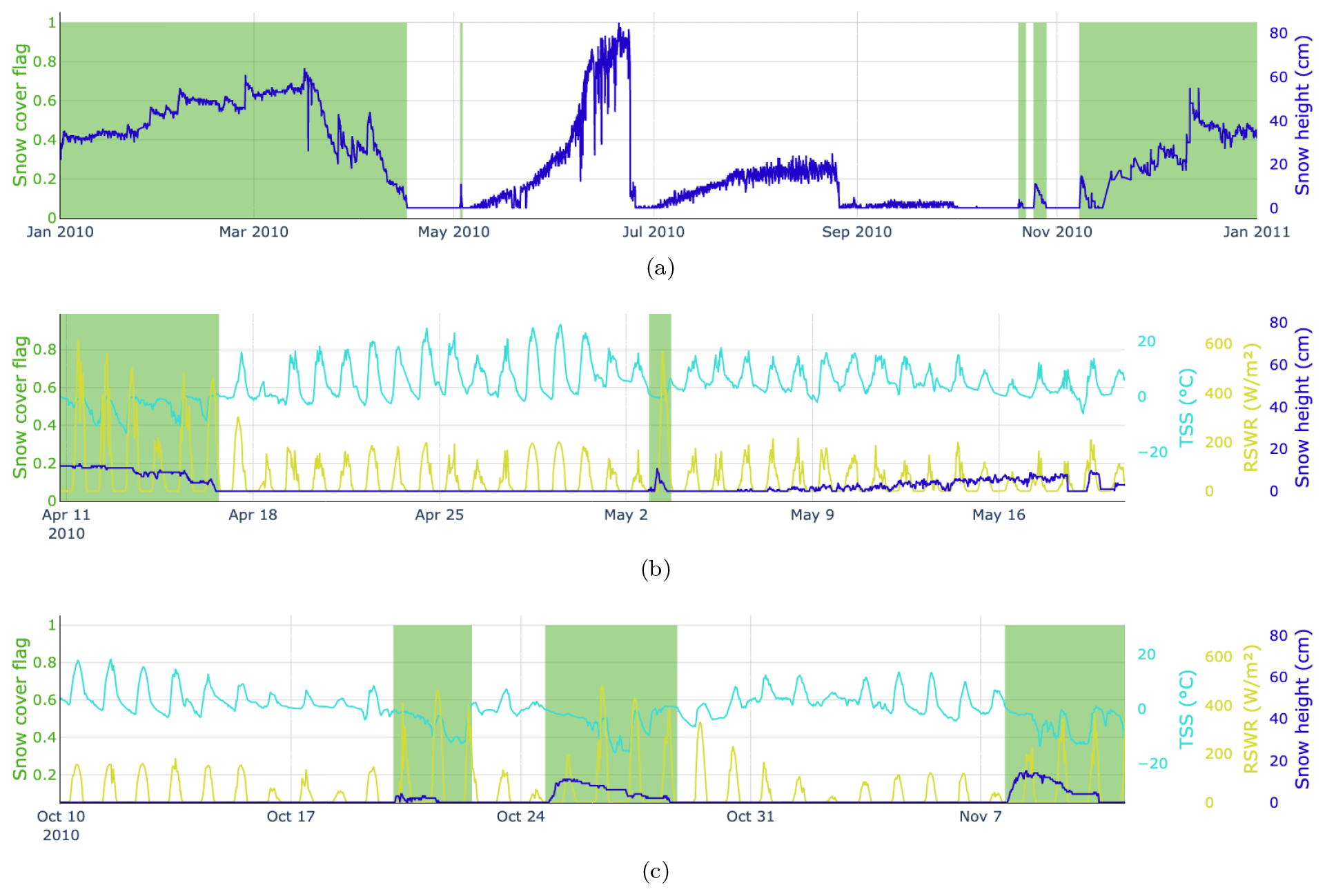
Figure 2 Examples of manually annotated data for the calendar year 2010 at station SLF2. Panel (a) shows the snow cover flag in green (1 for snow cover and 0 otherwise) and the snow height flag in blue for the whole year. Panel (b) focuses on the end of the winter season 2009/10, illustrating the diurnal behavior of TSS and RSWR depending on whether there is snow or not. Panel (c) is the same as panel (b) for the beginning of the winter season 2010/11.

2.1.2 Evaluation subset

We left some of the annotated data out during model development, which we later used as an independent test set to evaluate the generalization ability (e.g., Sect. 5.2 of Goodfellow et al., 2016) of our final approach at stations not seen at training time. We selected six stations (SLF2, WFJ2, KLO2, TRU2, STN2, and SHE2) that contain challenging scenarios and are therefore suitable test cases. In particular, these stations are located at elevations where summer snowfall occurs, the snow season duration is very different, or grass grows during the summer periods.

3 Methodology

To clarify whether snow or another ground cover is under a sensor, other sensor measurements can be used. To this end, a combination of seven input variables can be selected, i.e., HS, TA, TSS, RSWR, VW, RH, and solar altitude. We omitted TG, which was used during manual annotation, as it is not available at all IMIS stations and the sensor is also prone to defects. A detailed analysis of the input variable selection is provided in Sect. 4.1.3.

Looking at a data point in the context of its temporal neighborhood helps to determine whether there is snow or not at a particular time step. In an operational setting, one would, however, like to be able to make a prediction for each incoming data point in real time. This means that we cannot access data points in the future, and the context for each data point has to be composed of itself and the preceding data points (history). To reduce computational demands while still allowing for a large enough context, we suggest working with window sizes of between 8 and 192 time steps, where 1 time step corresponds to 30 min. The effect of varying time window size on the results is summarized in Sect. 4.1.4.

To account for the multivariate temporal characteristics of our data, we opted to use temporal convolutional networks, which have proven useful in many applications concerning time series (Wan et al., 2019; Pelletier et al., 2019; He and Zhao, 2019; Hewage et al., 2020). Later, Sect. 4.2 provides a comparison of CleanSnow with other popular models, such as random forests, MLPs, a variation of an RNN called an LSTM, transformers, and a recently released model for time series processing called TimesNet, which yields state-of-the-art results on various standard benchmarks.

3.1 TCNs

Based on well-known convolutional neural networks (CNNs) (Fukushima, 1988; Waibel et al., 1989; Weng et al., 1993; Lecun et al., 1998), TCNs are variations that consist of dilated, causal 1D convolutional layers that have the same input and output lengths. Dilation ensures that a specific entry in the output depends on all previous entries in the input, while causal convolution means that the ith element of the output sequence may only depend on input elements that come before it (elements with indices $\mathit{\{}\mathrm{0},\mathrm{\dots },i\mathit{\}}$).

As shown by Lea et al. (2016), with dilations and causal convolutions, TCNs can recover the behavior of RNNs while not suffering from typical drawbacks of RNNs, such as the vanishing gradient problem (Pascanu et al., 2013), and they are therefore easier to train. The use of convolutions instead of a recurrent mechanism also potentially leads to further performance improvements due to the possibility of parallelization of the convolution operation.

We chose a four-layer TCN architecture as shown in Fig. 3, which has 4D time series with 48 time steps as its input. The number of layers and filter sizes were selected so that the output representation of the last point in the input time series is an aggregation of all the previous time steps. In other words, the TCN produces an output representation of the last point in the input time series by aggregating information from the entire history that is available at input. This representation is fed into an MLP classifier, which first produces a series representation and then uses this representation to produce output class probabilities.

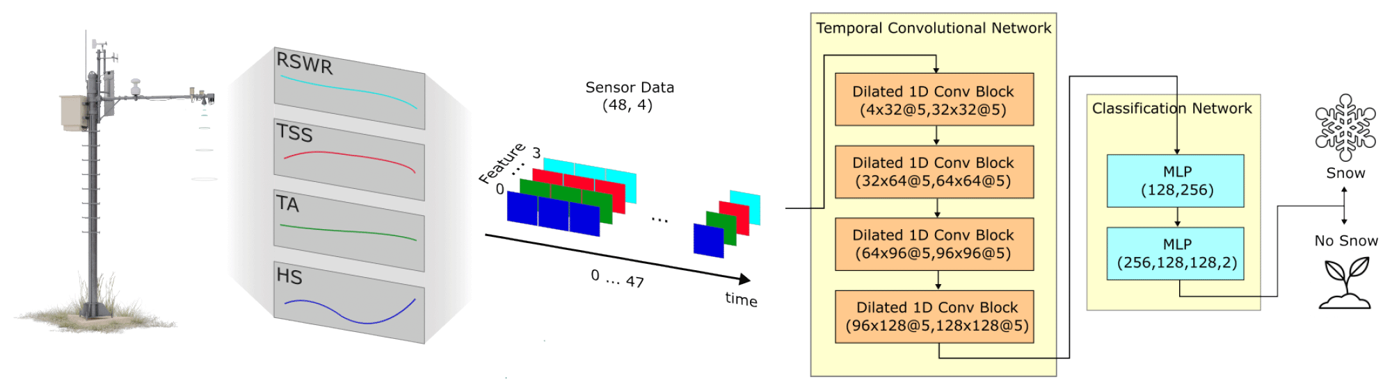
Figure 3 Flowchart of the proposed TCN-based architecture with a drawing of an IMIS station on the left. A time window of four input signals of length 48 (1 d) coming from an IMIS station is fed into the TCN, which causally aggregates information from all the time steps into a 128D latent vector. This information is subsequently fed into the classification network, which applies a sequence of MLPs to classify the input signal into two classes – Snow and No Snow. Each dilated 1D convolutional block has filters described in the format input_features × output_features @ kernel_size. The composition of each MLP is described as input_features, hidden_features_1$,\mathrm{\dots },$ output_features.

3.2 Training

Snow height classification is a binary problem. Binary classification problems are typically optimized using the cross-entropy loss function (Good, 1952), which did not yield good results in our case. Many of the stations included in the dataset are located in places where snow is present for much of the year, resulting in considerable class imbalance in our data. Moreover, we would like our model to perform well in the challenging marginal cases. Therefore, we chose to drive the optimization using the so-called focal loss (Lin et al., 2017), which allows the model to preferentially focus and train on examples that it has difficulty in classifying correctly while downweighting the simple cases throughout the training process.

The focal cross-entropy loss is defined as

$$\begin{array}{}\text{(1)}& {\displaystyle }{\displaystyle }\text{FL}=-\sum _{i=\mathrm{0}}^{N-\mathrm{1}}{\mathit{\alpha }}_i(i-p_i{)}^{\mathit{\gamma }}{\text{log}}_b(p_i),\end{array}$$

where α_i is the so-called balancing factor for class i, further contributing to class balancing; γ is the focus parameter which controls the downweighting of the easy examples; p_i is the probability of the sample belonging to the ith class; N=2 is the number of classes in the classification problem; and b is the logarithm base, which is typically b=10.

We run the training for a maximum of 300 epochs, feeding the model with a batch of 128 samples in each iteration. We allow for the possibility of early stopping if the validation loss has not improved for more than 50 epochs. The optimization process was governed by the AdamW (Loshchilov and Hutter, 2019) optimizer with an initial learning rate of 10⁻³. The learning rate was subject to step decay with a factor of 0.1, three times, after 50, 100, and 150 epochs.

3.3 Dataset

In all the experiments, we used the Snow and No Snow dataset described in Sect. 2.1.1. This dataset was split into training and evaluation subsets (see Sect. 2.1.2). For model training, we further (randomly) divided the training subset into two parts using a 90:10 split: 90 % used for training CleanSnow and 10 % for validation. The validation set was used to monitor CleanSnow's performance during training and hyperparameter tuning and enabled early stopping to prevent overfitting of the training data (Ying, 2019).

The whole training dataset contained approximately 7 million data samples, which would be rather impractical for experimentation, as it would yield extremely long training times and high computational demands that might not always be available. To make our experiments more tractable, we selected roughly 30 % of the data from every station in the training set using filtering by year (Table B1 shows which years were used from each station).

3.4 Hyperparameter tuning

We performed 5-fold cross-validation with random training–validation splits in order to perform hyperparameter tuning using a grid search for the following model architecture variables: dropout and output_activation for the TCN, batch_norm and activation_function for the MLP, and gamma and alpha for the focal loss and the optimizer learning rate.

For all of the remaining experiments, we have fixed a random seed for the training–validation split in order to ensure easy and full reproducibility of our results. Random splitting inherently takes care of having samples from different stations and different time periods throughout the whole training subset.

We opt for a batch size of 128 samples as this is sufficiently large while still fitting into the GPU memory we had available. Due to limited computing resources, we do not optimize the remaining hyperparameters, and we instead select them based on similar architectures available in other works and our experience with designing machine learning models.

4 Results

In this section, we summarize experiments performed to evaluate CleanSnow. With a series of ablation studies, we clarify various design choices and then compare our TCN, the model of choice, to other available options. We continue with a thorough evaluation of the TCN in different periods of the year, pointing out its strengths and weaknesses. The experiments are concluded with a case study that demonstrates the use of CleanSnow in vegetation science.

4.1 Experiments with the CleanSnow setup

In the following sections, different experiments with the CleanSnow configuration and model comparisons are shown to explain our design choices and their contributions to obtaining the best results. All the experiments were performed using a TCN with seven input features, i.e., HS, TSS, TA, RSWR, RH, WV, and solar altitude (which encodes information about the date and time of day).

The models were compared using the F1 score and the receiver operating characteristic (ROC) curve (Egan, 1975), which is a plot showing the performance in terms of the true positive rate (TPR), the false positive rate (FPR).

4.1.1 Synthetic ground truth experiments

To demonstrate the need for annotated data, we trained a model using a synthetic ground truth based on empirical rules developed according to human expert knowledge (see Appendix C). We compared the model trained with the synthetic ground truth information to the model trained with the manually annotated data. The results in Fig. 4a demonstrate the inability of thresholding rules to generate reliable ground truth information that could be leveraged for training. This resulted in the TCN synthetic ground truth model not learning the correct relationships between different input variables, yielding an F1 score of 93 % and therefore having a lower performance than the TCN manual ground truth model, which was trained with our manually annotated dataset and achieved an F1 score of 97 %.

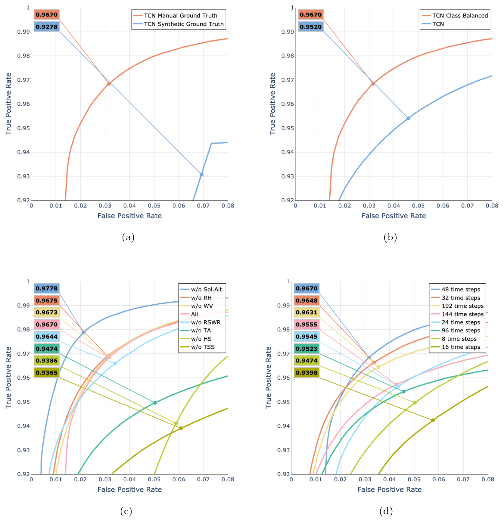
Figure 4 ROC curves for the various ablation studies. Every plot additionally shows the macro-F1 score for the threshold where TPR = FPR (the point on each curve). (a) Importance of manually annotated ground truth data. (b) Effect of class balancing. (c) Importance of input features. (d) Influence of sequence length on model performance.

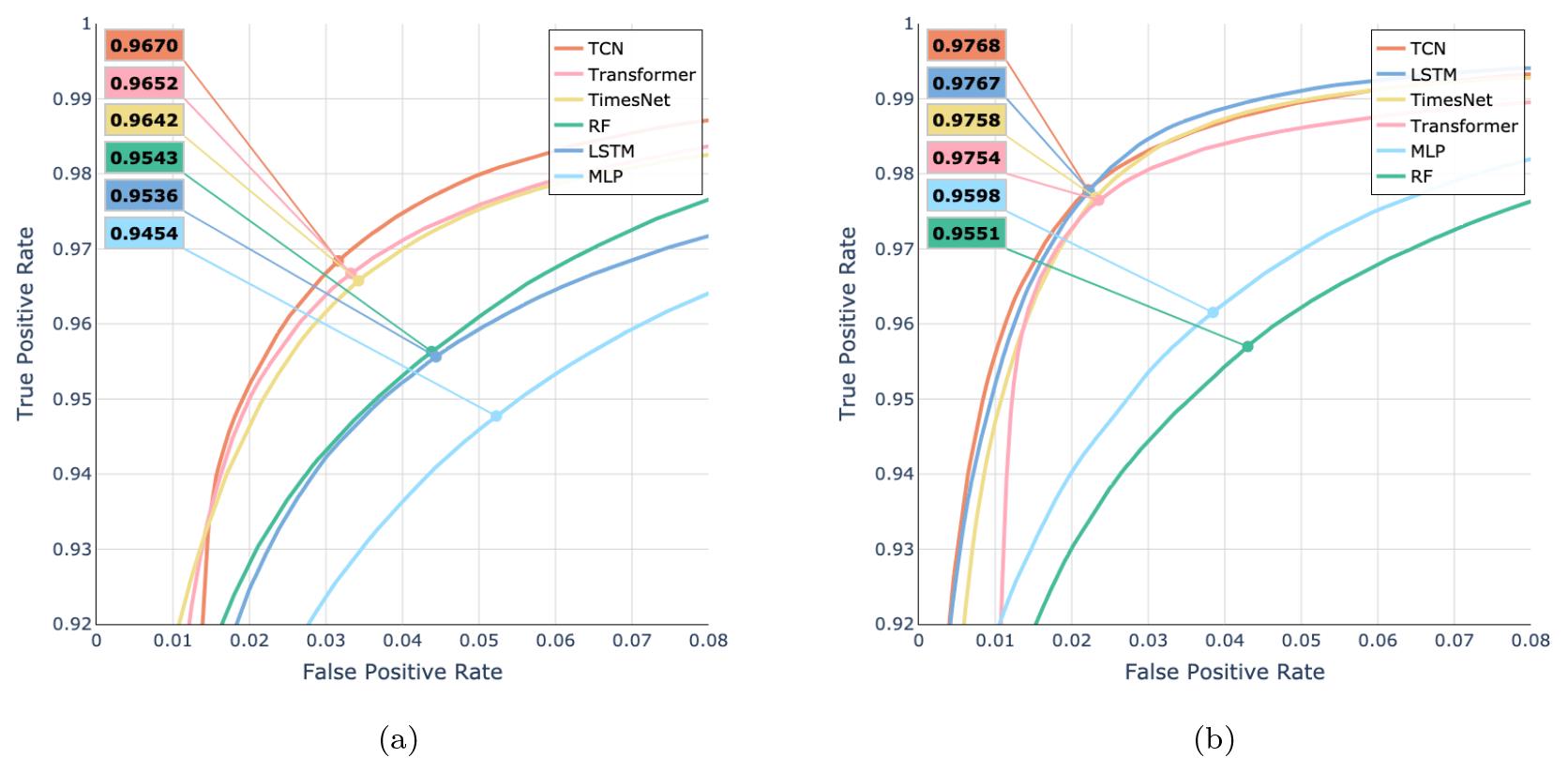
Figure 5 Model comparison shown as ROC curves for two different versions of the six models (LSTM, TCN, TimesNet, transformer, MLP, and RF): model performance with (a) all seven input features (HS, TSS, TA, RSWR, RH, WV, and solar altitude) and (b) the four relevant input features (HS, TSS, TA, and RSWR). Every plot additionally shows the macro-F1 score for the threshold where TPR = FPR (the point on the curve).

4.1.2 Class balancing

Our training dataset included roughly twice as many snow-covered samples as snow-free samples. We applied class balancing by adjusting the class weights of the focal cross-entropy loss and observed how that affected the performance of CleanSnow. We assigned a weight of 1.0 to the class representing snow and a weight of 0.5 to the class representing bare ground, as there are approximately twice as many data samples from the snow-covered period. Figure 4b shows that class balancing improved the performance from an F1 score of 95.2 % to one of 96.7 % and was therefore a valid design choice in our pipeline.

4.1.3 Feature importance

We conducted an ablation study training CleanSnow with a leave-one-out strategy for input features in order to validate their importance for model decision-making (Fig. 4c).

The HS, TSS, TA, and RSWR signals were found to be important (i.e., their removal resulted in a reduction in model performance with a decrease in the F1 score of up to 4 %), in line with what was discussed above for manual data annotation. On the other hand, removing WV and RH from the input features only marginally improved the model performance, suggesting that they have no positive effect. Hence, neither feature provided any additional information that was useful for classification. However, for other tasks, e.g., snow height anomaly detection, WV might very well be an important signal carrying information on snow transport by wind and related phenomena. Interestingly, removing solar altitude, which encodes information about the date and time, improved the performance of the model (increasing the F1 score by 1.5 %). We attribute this to the fact that solar altitude information potentially makes the model decide based on the date and time of the year, which is undesirable. As much as date and time data are generally valid indicators of the season and therefore have a strong influence on the presence of snow, they might hamper decision-making, especially at the beginning and end of the snow season and in the case of summer snowfall, whose occurrence varies from year to year.

Therefore, we chose our final model to have four input features, i.e., HS, TSS, TA, and RSWR.

4.1.4 Sequence length selection

One of the key parameters to choose is the length of the history the model can use to predict the current time step. Figure 4d shows the relationship between history length and model performance. The best results were obtained with a history length of 48 time steps (24 h), achieving an F1 score of 97 %. Very similar results were obtained with a history of length 32 (18 h) and an F1 score of 96 %. A history length shorter than 24 time steps deteriorated the performance, as did history lengths longer than 96 time steps. Accordingly, we set the history length to 48 time steps as a compromise between sufficient and not too much context for the model.

4.2 Model selection

To choose the right architecture for the task at hand, we experimented with several state-of-the-art machine learning models for single time step and time series processing, compared their performance, and finally selected the one that performed the best overall. Our model of choice was the TCN. A short description of the other models we evaluated is provided in Appendix D.

To have a balanced model that does not favor one of the classes, we selected the decision threshold as the point where TPR = FPR. We evaluated each model for two scenarios: one with all seven input features and one with only the four relevant features.

Figure 5 shows the overall best performance of the TCN with an F1 score of 97.8 %. Removing RH, WV, and solar altitude, which were identified as irrelevant features, resulted in a significant improvement of the LSTM model, equaling the performance of the TCN with an F1 score of 97.7 %. Nevertheless, we opted for the TCN, as it was on par with the LSTM, and the results in Fig. 5a suggest that the TCN is more resilient to unimportant features in the input. In addition, the TCN is known to be easier to train than LSTM. Interestingly, for RF the performance is less dependent on the selection of input features, suggesting its ability to deal with uninformative inputs.

4.3 Performance analysis per station

To better understand the generalization capabilities of the model, we evaluated its performance separately for each test station. The results in terms of confusion matrices are presented in Fig. 6 and suggest a good generalization capability of the model for most of the stations, except for SLF2 and STN2. Stations SLF2 (1563 m) and STN2 (2914 m) were considerably outside the elevation range that was available during the training. Moreover, these two stations are rather special cases compared to most of the other stations and can be considered out-of-distribution samples. Station SLF2 is located in a meadow in the village of Davos, which seems to have a positive effect on the classification as class No Snow, as it was the only station with an F1 score for class No Snow that was higher than for class Snow. Station STN2, by contrast, stands on a glacier, which results in very different ground properties compared to any other station in the dataset. This is reflected in a lower F1 score for class No Snow, especially as STN2 reached an F1 score of only 94.5 % (which is 2 % less than any other station in the test set). In addition, from Figs. 6 and 7, one can further conclude that the model generally classifies the presence of snow slightly better than the absence of snow.

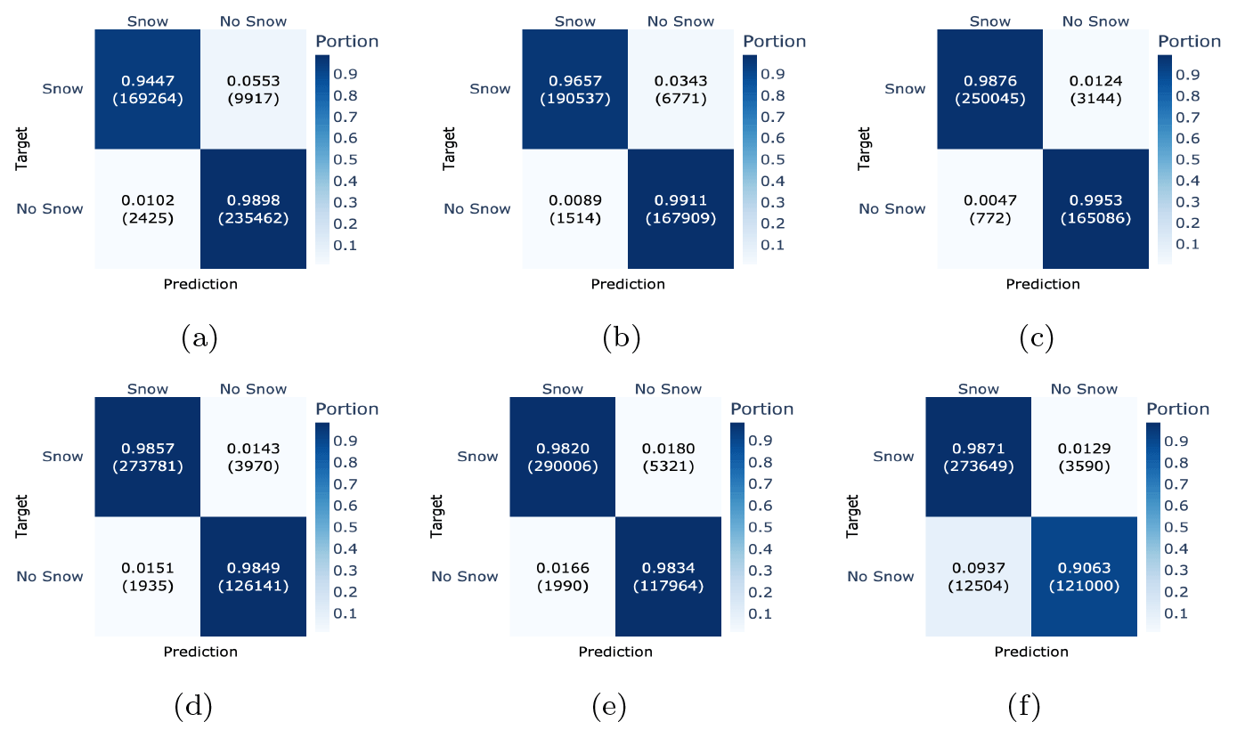
Figure 6 Performance evaluation of each test station separately, shown in terms of confusion matrices ordered by elevation (a–f): SFL2 (1536 m), SHE2 (1852 m), KLO2 (2147 m), TRU2 (2459 m), WFJ2 (2536 m), and STN2 (2914 m). Each confusion matrix has targets as rows and predictions as columns.

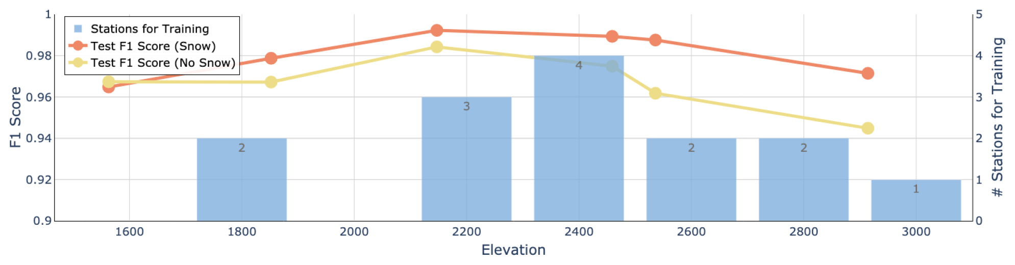
Figure 7 Model performance for the six stations in the test subset as a function of elevation. The F1 score is shown separately for the classifications Snow (red line) and No Snow (green line). The blue columns indicate the elevation distribution in the training subset (14 stations).

It is also important to understand whether CleanSnow generalizes to stations at different locations with different elevations. The results presented in Fig. 7 suggest that the model performance was very stable for stations at elevations between about 2100 and 2700 $\mathrm{m}\mathrm{a}.\mathrm{s}.\mathrm{l}.$, while it decreased for stations located either below or above this range. This corresponds to the fact that 80 % of the stations in our training set were in this range, only two were below 2000 m, and one was at 2800 m.

The seemingly good performance of the model should however be analyzed in detail. There are periods for which it is rather easy to correctly classify snow as Snow and snow-free ground as No Snow, together with other times of the year when the problem becomes much harder. This is discussed in detail later in Sect. 4.4.

4.4 Performance for different times of the year

Classification of snow height measurements into snow and snow-free ground can be both a simple and rather challenging task, depending on the location and time of year. We provide a per-month performance analysis in Fig. 8, which shows that the model mostly had trouble predicting snow-free ground in the winter months. This is because very few training data for that class were available during December, January, February, and March. Furthermore, we had no snow-free samples in the test set for February and March. In summer, instead, the results suggest that CleanSnow was able to detect most of the summer snowfall (with a performance drop of approximately 20 % compared to the full winter) while maintaining very good performance in predicting snow-free ground. At the end of winter, in May and June, the model performance was also very good, suggesting that CleanSnow can be used to accurately predict the snow disappearance date (as a longer snow-free period after a long period with constant snow cover).

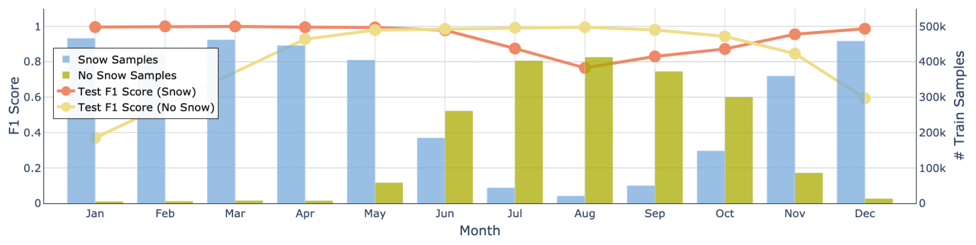
Figure 8 Performance of the model for each month of the year. The F1 score is shown separately for the classifications Snow (red line) and No Snow (yellow line). The blue columns indicate the distribution of the Snow samples, while the yellow columns indicate the distribution of the No Snow samples.

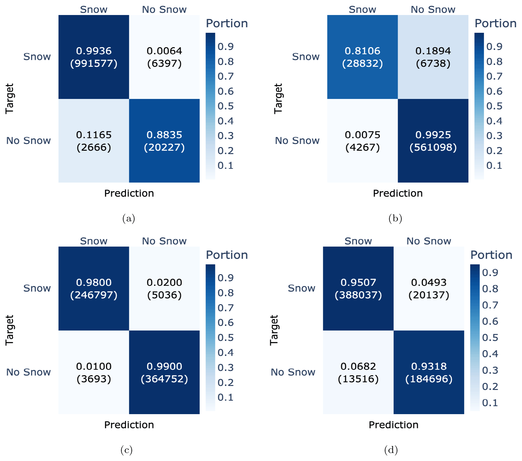
Figure 9 Confusion matrices for each of the four seasonal clusters: (a) winter season (December–April), (b) summer season (July–September), (c) end of the winter season (May–July), and (d) start of the winter season (October–December). Each confusion matrix has targets as rows and predictions as columns.

In addition, we analyzed the model performance for each season. To this end, we split the test dataset into four different seasonal clusters:

• The winter season was defined as the period with mostly continuous snow cover (December, January, February, March, and April).

• The summer season was the part of the year typically without snow (July, August, and September).

• The end of the winter season was defined as the snowmelt period resulting in snow-free ground (May, June, and July).

• The start of the winter season included the months when it starts snowing more often and at some point a continuous snow cover forms on the ground (September, October, and November).

In the following sections we describe the model performance for each of the four seasonal clusters in detail and point out some season-specific challenges.

4.4.1 Winter season

For snow classification, the middle of winter is presumably the easiest time of the year. Besides some low-elevation stations and some exceptional seasons with a very late onset of winter or very early snowmelt, the task should be rather trivial, as the snow cover is continuous in time. Figure 9a demonstrates that the model confidently classified snow (TPR = 99.4 %), in contrast to snow-free ground (TPR = 88.4 %).

4.4.2 Summer season

In contrast to the full winter, the classification of snow in summer is more challenging. Besides snow-free ground, there were many stations where vegetation grew (approximately 20 % of the data in the test set). This resulted in nonzero snow height sensor measurements, which do not correspond to snow. Exceptions were stations at high elevations (e.g., on a glacier) and winters when the snow did not melt until the beginning of summer.

The snow height signal for snow-free ground typically oscillates with high frequency and either stays around zero or grows in the presence of vegetation under the sensor. The surface temperature and air temperature will most of the time oscillate high above 0 °C, showing a diurnal cycle. During overcast periods or in the presence of precipitation, TA and TSS will show the same value. Due to the lower albedo of snow-free ground, smaller amounts of RSWR are measured. Based on the above assumptions, summer snowfall can be detected when TA equals TSS, which is followed by larger values of RSWR with a simultaneous decrease in TSS. If there is vegetation growing under the station, the HS signal counterintuitively decreases as the plants are pressed down by the snow. In the case of snow-free ground under the sensor, the HS signal will increase as expected during snowfall.

Figure 9b demonstrates that the model accurately detected snow-free ground with 99 % accuracy. The effect of summer vegetation is shown in Fig. 10a. On the other hand, detecting snowfall in the summer proved to be difficult, and even more so when vegetation was present. In this very difficult setting, CleanSnow achieved a performance of 81 %. A partial detection of summer snowfall is shown in Fig. 10c. CleanSnow succeeded in detecting the main event but failed to correctly classify a few hours at both the start and end of the summer snowfall.

4.4.3 Start and end of the winter season

The transition periods between winter and summer and vice versa are key periods for the detection of the first snow and its disappearance, which are both dates of interest in climate science. These two seasonal clusters contain both data with rather continuous snow cover and data with bare ground or vegetation growth. Such data are therefore a perfect test case for CleanSnow.

In our experiments, the end of the winter season was the easier case to classify, achieving very competitive performances of 98 % for snow and 99 % for snow-free ground (Figs. 9c and 10). We attribute this high accuracy to the fact that the transition from snow-covered to snow-free ground was often rather smooth, and once the snowpack melted there were not many periods with snow persisting on the ground. The beginning of summer was typically represented by high air temperatures, which caused TSS to oscillate with the daily cycle, indicating snow-free ground. Simultaneously, RSWR noticeably decreased once the snow had completely melted.

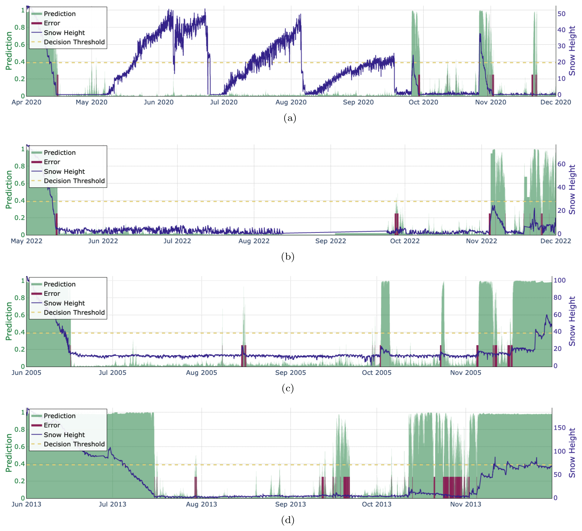
Figure 10 Examples of CleanSnow classification results. The snow height signal is depicted in blue. The model predictions in terms of probability (0–1) are shown in green. The dashed horizontal line denotes the decision threshold selected to balance the model performance in predictions for both classes. The red-shaded areas mark regions with classification errors (i.e., samples assigned to the wrong class). (a) SLF2 (1563 m), year 2020 shows a correct classification of summer vegetation growth (the nonzero blue curve is classified with a probability lower than that of the decision threshold and therefore is assigned to class No Snow). (b) SHE2 (1852 m), year 2022 is an example of early October snowfall that has been classified partially correctly. (c) TRU2 (2459 m), year 2005 demonstrates the model's ability to detect summer snowfall and scattered snowfall at the beginning of winter. (d) STN2 (2914 m), year 2013 is evidence that the model does not always perform well, here making mistakes at the beginning of the next winter season.

On the other hand, classification at the start of the winter season was more challenging: the model achieved accuracies of 95 % for snow and 93 % for snow-free ground (Figs. 9d and 10). There were multiple cases of snowfall at the beginning of the season, after which the snow melted again completely. In addition, in late fall and at the beginning of winter, temperatures occasionally dropped and the ground froze overnight. This resulted in TSS being constantly less than or equal to 0 °C even without snow, which might force the model to focus more on RSWR and HS during decision-making, potentially decreasing its decision-making power.

4.5 Comparison with manual observations

Perfect test cases are stations with concurrent manual observations, i.e., measurements performed manually by human observers. Such measurements were available for the two stations WFJ2 and SLF2 located in the region of Davos.

Since the manual measurements were taken only once a day, we resampled our predictions from 30 min intervals into 24 h intervals. We averaged probability scores over the 24 h (48 automatic measurements) to obtain the per-day probability score.

The performance comparison of annotated automatic measurements and manual observations in Fig. 11 confirms that we produced high-quality annotations for the historical data. Some days with snow were erroneously annotated as snow-free ground. This can be related to both short snowfall which disappears in daily aggregation and the fact that manual observations were performed around 08:00 CET in the morning, while our data were daily averaged values. Such misalignment might produce additional disagreements between manual observations and our annotations.

The results also show that CleanSnow achieved a very good performance when evaluated against daily manual observations. The differences in performance between the two ground truth sources (approximately 2 % in TPR and 1.5 % in TNR) were attributed to the inconsistencies between the manual annotations of automatic measurements and manual observations.

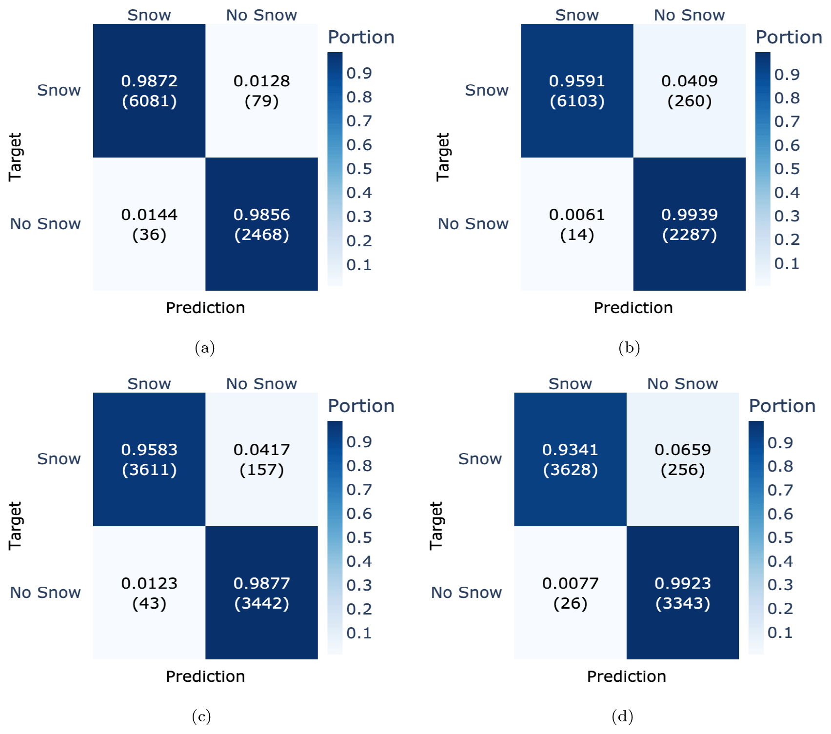
Figure 11 Confusion matrices for comparison of model performance evaluated against our annotations (left) and against human observer measurements (right). The results for station WFJ2 are in (a) annotations and (b) observations, followed by the results for SLF2 in (c) annotations and (d) observations.

4.6 Comparison with other approaches

To further demonstrate the added value of our machine learning approach, we compared it with other state-of-the-art methods such as filtering used in the physics-based snow cover model SNOWPACK (Lehning et al., 1999). In particular, we considered SWE provided by SNOWPACK since the HS signal is filtered to calculate SWE. Therefore, SWE should be a good indicator of whether the HS signal relates to snow or not. If the HS signal does not represent snow, one would expect SWE to be 0. In addition, we compared CleanSnow to thresholding-based filters implemented in the MeteoIO library, which were mainly designed to filter vegetation growth measurements in summer.

Figure 12 shows a comparison of the snow height classification by our TCN model with classification based on SWE calculated by SNOWPACK and the MeteoIO filter. The results suggest that the machine learning approach is superior in most cases. This might be due to the fact that both SNOWPACK and MeteoIO use thresholding-based rules based on TSS and TG to filter HS similarly to the approach described by Tilg et al. (2015). The optimal threshold values vary across different stations, which requires per-station calibration of the thresholds. Moreover, TG-based filtering is problematic since, as already mentioned, the TG sensor is prone to failures and the signal is therefore often missing at some stations.

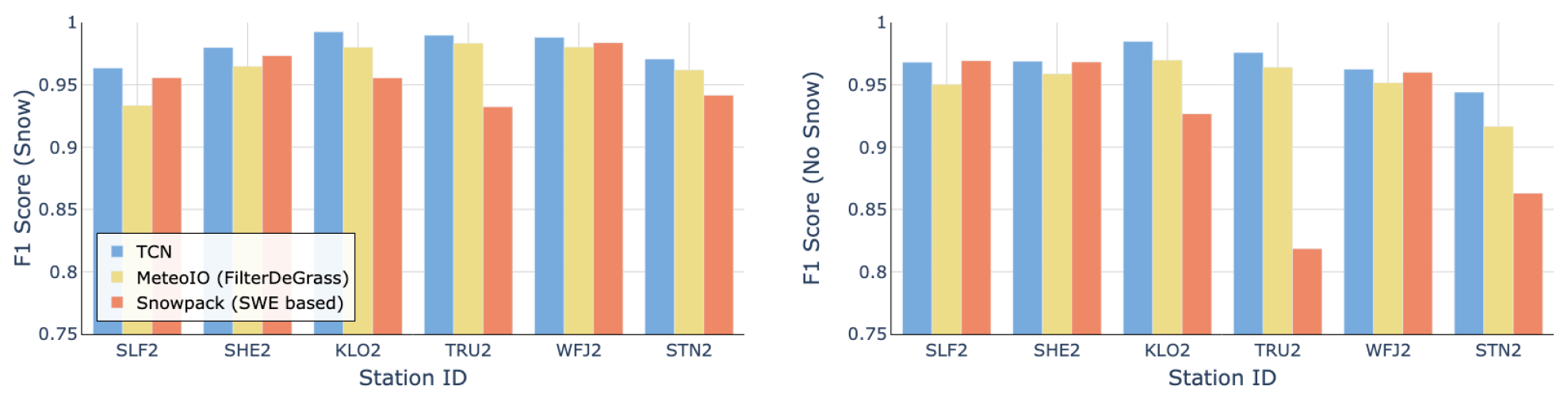
Figure 12 Comparison to other approaches shown as performance (F1 score) per station for CleanSnow (blue), the filter based on the SWE from SNOWPACK (red) and the thresholding filter from MeteoIO (yellow).

4.7 Case study: vegetation growth

Besides obvious applications in snow science, reliable separation of snowfall from plant growth has benefits for biological research. Removing HS measurements classified as snow allows for the extraction of a clean vegetation signal and the pinning down of reoccurring events in the life cycle of alpine vegetation – referred to as vegetation phenology. Since snow and plant heights have been recorded for a very long time, it is possible to relate the timing of green-up (i.e., the start of vegetation growth) or other phenological phases to snow climate parameters and study phenological shifts over time – an excellent indicator of climate change (e.g., Inouye, 2022). We extracted 25 years of vegetation growth data from HS measurement data at TUJ2 (Culmatsch, 2262 $\mathrm{m}\mathrm{a}.\mathrm{s}.\mathrm{l}.$), an IMIS station characterized by tall plant growth. Within the 20 years of data, the algorithm flagged all snow days during the vegetation period, which were then removed. Snow disappearance and snowmelt dates were defined as the first and last days of continuous winter snow cover. We fitted a logistic growth curve (Kong et al., 2022) to the clean plant growth measurements and defined the start of growth as a 10 % threshold of maximum plant height (Fig. 13). Vegetation green-up was directly linked to the timing of snowmelt, consistent with other studies (Jerome et al., 2021; Jonas et al., 2008), while late snowfall events shifted the start of growth towards later calendar days. Linear regression analysis revealed an earlier occurrence of green-up over the study period, coinciding with an increase in spring temperatures measured at the station. Despite insignificant changes in snowmelt timing, the shorter lag between snowmelt and the initiation of plant growth suggests a warming-driven advancement in phenology at the study site. This case study highlights the importance of long-term monitoring and automated machine learning approaches in understanding climate-induced phenological shifts, with implications for ecosystem dynamics in remote alpine regions.

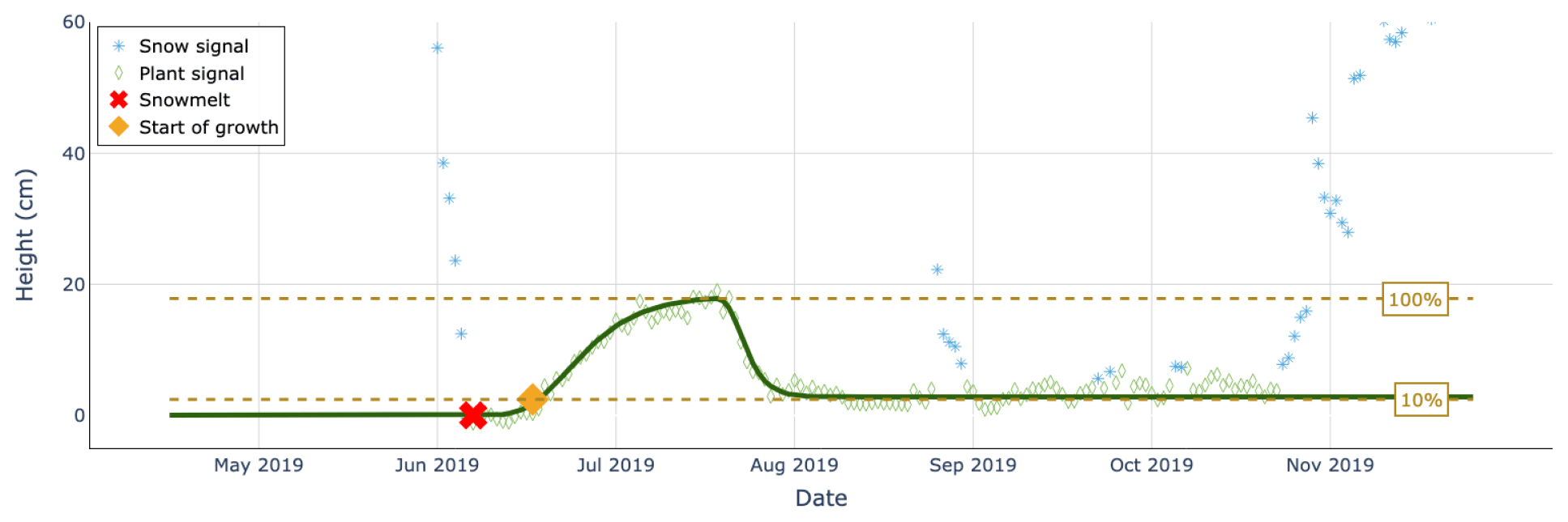
Figure 13 An example of a logistic growth curve (in dark green) fitted to height measurement data from TUJ2 in the vegetation season of the year 2019. Snow height data corresponding to snow are shown with blue stars, while the plant signal is shown with green diamonds. The red cross marks the snowmelt date, while the orange diamond marks the start of plant growth.

5 Discussion

We proposed a deep-learning-based approach to snow height signal classification, which is a crucial step in automating the snow height signal quality-checking process. In addition to selecting an appropriate model, we provided some good practices to develop machine learning models for automated snow height classification.

5.1 Best practices for snow height classification using machine learning

In our analysis, we aimed to establish best practices for further development of machine learning methods for snow height classification and quality assessment. We showed that learning from synthetic ground truth data generated using thresholding rules proposed in the past did not work well, as the predefined thresholds did not generalize to all stations without modifications. This emphasizes the need for well-annotated data for training. Next, we pointed out the importance of addressing the class imbalance problem to achieve the best possible performance. Furthermore, we demonstrated the superiority of sequence-based models (TCNs, LSTM, TimesNet, and transformers) to single time-step-based models (RF and MLP), which confirms the need for temporal context to achieve a high classification performance. We acknowledge the existence of techniques that allow one to feed RF and MLP models with sequences of data, e.g., lagged features (i.e., adding data from previous time steps as extra input features). Nevertheless, we argue that such techniques do not treat sequential data as a causal sequence, which is conceptually nonideal and might potentially lead to the resulting model becoming less explainable in how it treats temporal information. Another important aspect to consider is the sequence length. We performed an analysis of the performance for the length of the time window (i.e., the size of the temporal context), which revealed that the ideal length was around 48 time steps, as shorter and longer time windows resulted in a deterioration of the model performance. Subsequently, we showed that it was important to evaluate the model performance during the critical times of the year (the start and end of the winter season) to reveal the true performance.

5.2 Deep-learning models for snow height classification

We studied the suitability of state-of-the-art deep-learning models for the snow height classification task. Several cutting-edge deep-learning architectures have been evaluated against each other, resulting in the superiority of a TCN to the other compared methods. CleanSnow reached an accuracy of 97.7 % in the independent test set when we used a decision threshold that balanced the model performance of predictions for both classes – Snow and No Snow. Hence, the results indicate that the approach generalizes well to unseen stations that are within the distribution of the training set. A detailed performance evaluation for each station in the test set showed that the model performed very well, except for the data of stations SLF2 and STN2, which are two particular cases that were not represented well in the training data. Station SLF2 is located low in a valley, and STN2 is on a glacier. In addition to being out-of-distribution, such special environments, compared to those of most other stations in the dataset, might cause slightly different behavior of the auxiliary variables used during HS analysis and result in a performance decrease.

5.3 Generalization

The generalization ability of CleanSnow to elevations that are within the range included in the training set is good. These elevations represent the Alps, which is the region of interest for us. Generalization to out-of-distribution samples (stations located at elevations that are not represented well in the training data) is rather poor. Out-of-distribution generalization, however, remains an open problem in the machine learning community. One possibility for improving out-of-distribution generalization is to explicitly express some known behavior (e.g., physical constraints) in a neural network. Such models are known as physics-informed neural networks (PINNs) (Raissi et al., 2019) and can be implemented by either adding a regularization term to the loss function or incorporating the constraints directly into the model architecture. In both cases, such constraints help the model to correctly extrapolate to situations that were not represented in the training data.

5.4 Limitations

One of the known limitations of CleanSnow is the fact that it operates on raw data, meaning that the inputs may contain both anomalies (e.g., spikes) and missing values. Even though CleanSnow seems to be resilient to anomalies, it would be good practice to perform anomaly detection and filtering before running the proposed snow height classification models. We argue that filtering obvious spikes in the snow height signal is a rather trivial procedure and can be solved by employing statistical methods such as Hampel filtering (Pearson, 1999) or an exponential moving average filter (Kendall and Stuart, 1966). However, other, more subtle variations are very challenging to detect by both the human eye and automated methods.

CleanSnow can only be applied in cases where the full history needed to make a prediction is available. At the moment, in the case of missing samples in the context of 48 time steps, the samples are discarded without being run through the model. Dealing with missing data is far more complicated than filtering anomalies. A simple solution for periods of up to several time steps would be linear interpolation. However, as the size of the interpolated interval increases, this fails to produce an accurate reconstruction of the missing data. To impute longer periods of missing data, methods that take into consideration both spatial and temporal contexts should be employed. This is, however, beyond the scope of this work, and we therefore leave it as a possible future research direction.

6 Conclusions

Automated snow height measurements are key input data for many modeling approaches in climate science, snow hydrology, and avalanche forecasting. Erroneous snow height measurements deteriorate the performance of these models. We demonstrated how to mitigate the aforementioned issues through the use of deep-learning methods for automated snow height classification. Our contributions can be summarized as being three-fold. First, we created a novel machine learning approach to snow height signal classification that operates directly on time series data. Second, we provided an in-depth comparison of several machine learning models applied to snow height classification. Third, we introduced a new benchmark dataset with annotated snow height data, which sets a baseline and can be used for further research in the field. The proposed approach achieved a high accuracy of 97.7 % and generalized well to previously unseen stations. CleanSnow can be implemented as a component of an arbitrary snow height quality assessment pipeline without the need for any special hardware.

Appendix A: List of stations in the Snow and No Snow dataset

This section provides a list of IMIS stations used in our Snow and No Snow dataset (see Sect. 2.1.1), together with their metadata. Table A1 shows the stations ordered by increasing elevation. The column “Subset” indicates whether a station was used for training or testing.

Table A1 List of stations that are part of the Snow and No Snow dataset, together with their auxiliary information, ordered by elevation. The column “Subset” denotes whether a station belongs to the training set or test set.

Appendix B: Subsampling of the training data

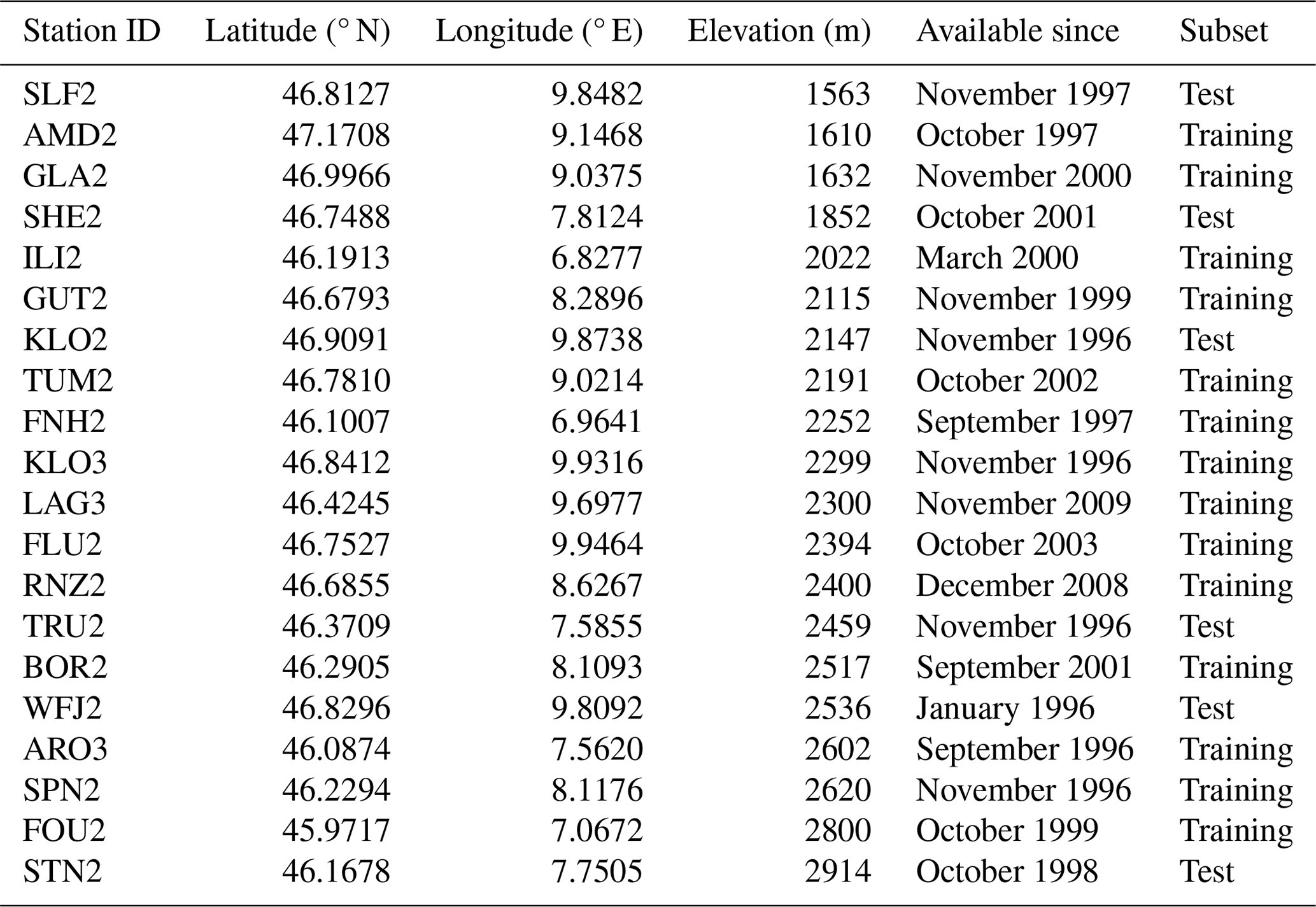
Table B1 List of years for each station that were selected as part of the subsampled training dataset.

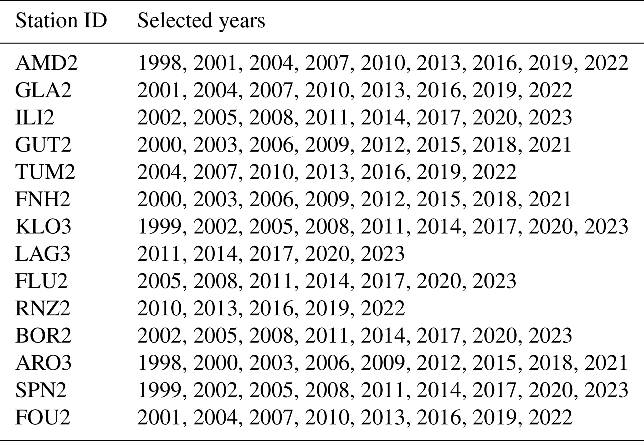
To run experiments in a reasonable time and make sure that they were computationally tractable, we subsampled the training dataset to reduce the number of training samples. In Table B1, we list which years were selected for each station for the training set.

Appendix C: Synthetic ground truth generation

We generated synthetic ground truth data by applying thresholding rules inspired by the works of Bavay and Egger (2014) and Tilg et al. (2015) to the HS measurements. In order for a sample to correspond to snow cover, the following condition had to be met:

$$\begin{array}{}\text{(C1)}& {\displaystyle }\begin{array}{rl}{\displaystyle }& {\displaystyle }\left(\left({\displaystyle \frac{\mathrm{1}}{N}}{\sum }_{n=\mathrm{0}}^{N-\mathrm{1}}{\text{TSS}}_n\right)\le \mathrm{0.0}\right)\wedge \\ {\displaystyle }& {\displaystyle }\left(\left({\displaystyle \frac{\mathrm{1}}{N}}{\sum }_{n=\mathrm{0}}^{N-\mathrm{1}}{\text{RSWR}}_n\right)\ge \mathrm{300.0}\right),\end{array}\end{array}$$

where N is the length of the time window.

Appendix D: Machine learning models

For completeness, we provide a short description of every machine learning model that was used in our performance comparison.

D1 RF

Implemented in many data science libraries and easy to use, RF is a popular choice of machine learning algorithm that can provide satisfactory predictions in both classification and regression tasks. In practice, RF is an ensemble approach, which produces a final prediction as a combination of outputs of many decision trees. It often works well on tabular data, but there are no mechanisms that would allow for a more principled representation of temporal, spatial, or graph structures.

In our experiments we used the RF classifier implementation from the scikit-learn library (Pedregosa et al., 2011), setting the number of decision trees to 1000 and the maximum depth of each tree to 50. We left the other parameters at their default settings and trained the RFs using the Gini criterion (Gini, 1921).

D2 MLP models

Being one of the first neural network models that can learn nonlinear functions, MLPs have shown their power in natural language processing (NLP) and serve as a foundational component of many other current neural network models. Finding their applications in both regression and classification tasks, MLPs can serve as an alternative to the RFs presented above. Putting them in comparison with RFs, MLPs can be generally more difficult to train for a given task and often exhibit lower performance, especially with tabular data. This is due to their nature of learning smooth (sometimes overly smooth) solutions, thereby causing them to not perform well for problems with a non-smooth decision boundary. Grinsztajn et al. (2022) argue that this is due to the gradient descent approach to MLP optimization. They also show that MLPs are more affected by, e.g., uninformative features compared to RFs.

We designed an MLP composed of an input layer with seven input dimensions and 32 output features, followed by three hidden layers with 64, 128, and 256 output features, respectively. Each hidden layer had batch normalization (Ioffe and Szegedy, 2015) and rectified linear unit (ReLU) activation functions (Fukushima, 1969; Nair and Hinton, 2010) appended to it. The MLP was concluded with an output layer which takes a 256-feature representation and produces the final class probability score.

D3 LSTM

Belonging to the family of RNNs, the original models developed for time series processing, GRU (Cho et al., 2014) and LSTM (Hochreiter and Schmidhuber, 1997) are variations that allow models to better capture long-term dependencies compared to RNNs, which tend to forget inputs that came much earlier in the history. We chose to use LSTM in our experiments, as it is one of the gold standards in deep learning for time series processing.

The LSTM model we used in our experiments took an input with seven dimensions and was composed of three recurrent layers with hidden dimensions of 64, 128, and 256, followed by an output MLP classifier that produced the final probability scores.

D4 TimesNet

Recently released and setting the new state-of-the-art performance for many standard benchmarks, TimesNet (Wu et al., 2023) has become one of the models of choice for time series processing in general. Its main characteristic is the transformation of a 1D time series signal into a 2D one, which allows it to capture complex temporal variations in the signal. The conversion of a time series into a 2D signal is based on detecting signal periods using amplitude information from a fast Fourier transform (FFT) and ordering the signal chunks into a 2D array. Applying 2D convolutions to this array allows it to capture both inter- and intra-period variations in the signal.

In our experiments we used a modification where the definition of signal periods is fixed and not determined by the FFT. We used five periods to split the signal, i.e., 48, 32, 24, 16, and 8. The model was then composed of three layers, with each layer having two blocks and 128 hidden features.

D5 Transformers

Since they were published in 2017, transformers have revolutionized many areas of deep learning, achieving new state-of-the-art results, mostly in natural language processing and computer vision. Transformers are models based on an attention mechanism (Vaswani et al., 2017) and were originally proposed for sequence-to-sequence tasks.

Here we employed a modification of the traditional transformer. In particular, we took the classical transformer encoder in order to produce a latent representation for the input sequence, where each point is conditioned on the past context. The encoder was composed of two layers with hidden dimensions of 128 and four attention heads. Both the input positional encoding and the encoder have a dropout of 0.1 applied. The latent representation produced by the transformer encoder was average-pooled and passed to an MLP readout network, which produced the classification probability scores.