the Creative Commons Attribution 4.0 License.
the Creative Commons Attribution 4.0 License.
 | 13 Mar 2025
Long-term hydro-economic analysis tool for evaluating global groundwater cost and supply: Superwell v1.1
Stephen B. Ferencz
Neal T. Graham
Thomas B. Wild
Mohamad Hejazi
David J. Watson
Chris R. Vernon
Groundwater plays a key role in meeting water demands, supplying over 40 % of irrigation water globally, with this role likely to grow as water demands and surface water variability increase. A better understanding of the future role of groundwater in meeting sectoral demands requires an integrated hydro-economic evaluation of its cost and availability. Yet substantial gaps remain in our knowledge and modeling capabilities related to groundwater availability, recharge, feasible locations for extraction, extractable volumes, and associated extraction costs, which are essential for large-scale analyses of integrated human–water system scenarios, particularly at the global scale. To address these needs, we developed Superwell, a physics-based groundwater extraction and cost accounting model that operates at sub-annual temporal and at the coarsest 0.5° (≈50 km × 50 km) gridded spatial resolution with global coverage. The model produces location-specific groundwater supply–cost curves that provide the levelized cost to access different quantities of available groundwater. The inputs to Superwell include recent high-resolution hydrogeologic datasets of permeability, porosity, aquifer thickness, depth to water table, recharge, and hydrogeological complexity zones. It also accounts for well capital and maintenance costs, as well as the energy costs required to lift water to the surface. The model employs a Theis-based scheme coupled with an amortization-based cost accounting formulation to simulate groundwater extraction and quantify the cost of groundwater pumping. The result is a spatiotemporally flexible, physically realistic, economics-based model that produces groundwater supply–cost curves. We show examples of these supply–cost curves and the insights that can be derived from them across a set of scenarios designed to explore model outcomes. The supply–cost curves produced by the model show that most (90 %) nonrenewable groundwater in storage globally is extractable at costs lower than USD 0.57 m−3, while half of the volume remains extractable at under USD 0.108 m−3. The global unit cost is estimated to range from a minimum of USD 0.004 m−3 to a maximum of USD 3.971 m−3. We also demonstrate and discuss examples of how these cost curves could be used by linking Superwell's outputs with other models to explore coupled human–environmental system challenges, such as water resources planning and management, or broader analyses of multisectoral feedbacks.
- Article
(10608 KB) - Full-text XML
-
Supplement
(9849 KB) - BibTeX
- EndNote


The second half of the 20th century saw a global proliferation of groundwater extraction that played a significant role in meeting regional water demands associated with population growth, economic development, and agricultural production (Konikow and Kendy, 2005; Jasechko et al., 2024). Groundwater use has continued to steadily rise in many regions (Jasechko and Perrone, 2021; Bierkens and Wada, 2019; Grogan et al., 2017), with projections suggesting a potential peak in global extraction by 2050, followed by a decline through 2100 (Niazi et al., 2024c). Groundwater also provides a critical though sometimes costly buffer against drought by supplementing surface water during periods of short-term deficit (Siebert et al., 2010). Reliance on groundwater to meet demands for irrigation, as well as for the municipal and industrial sectors (Scanlon et al., 2023; Müller Schmied et al., 2021), combined with an anticipated increase in the variability of surface water supplies due to climate change (Schewe et al., 2014), raises questions about how groundwater availability and use will evolve over the 21st century; which regions may experience groundwater depletion; and what are the effects of groundwater depletion on regional economic growth, trade, and water security.
Addressing these types of societally consequential questions requires an integrated analysis of human–water systems. Such analysis in turn requires knowledge of both the spatiotemporal distribution of water and its economic characteristics, which can shape human water usage patterns. Relative to surface water, groundwater is distinct in the complexity of its distribution of stocks and flows and its economic cost characteristics. While far more data collection and modeling have been dedicated to human interactions with surface water, new classes of integrated modeling tools have emerged that are capable of exploring groundwater's broader interactions with key human systems. These include human–Earth system models designed to explore multiscale, multisector dynamics (Keppo et al., 2021) at a global scale as well as hydro-economic (Harou et al., 2009) and agent-based models (Castilla-Rho et al., 2017; Yoon et al., 2021; Klassert et al., 2023) designed to explore regional and local-scale coupled human–groundwater systems. These classes of models differ in numerous respects, particularly the spatial domains and processes they include. However, a common thread among these models is that they can benefit, either in practice or in theory, from improved information about the physical availability of groundwater and its cost characteristics.
Global multisector dynamic models enable exploration of various long-term scenarios to gain insight into the co-evolving interactions among socioeconomic, climate, and energy–water–land systems (Keppo et al., 2021; Weyant, 2017; Fisher-Vanden and Weyant, 2020). Models in this class vary considerably with regard to their representation of surface and groundwater resources, as well as whether and how the economic costs of water extraction are accounted for (Keppo et al., 2021; Wild et al., 2023). Despite the substantial differences among models within this class, they often constrain the level of detail with which individual systems are modeled to allow for greater focus on their interactions. In other words, these models typically seek to include coarse representations of water resource availability and costs (e.g., for groundwater), in order to explore future water usage and its broader economic consequences (Dolan et al., 2021). For instance, such availability–cost relations could be used in models like the Global Change Analysis Model (GCAM) to analyze future demand-driven groundwater withdrawals (Niazi et al., 2024c) or explore how groundwater depletion during the 21st century could affect food production in different regions of the world and shift cropping patterns from irrigated to rainfed (i.e., non-irrigated) (Turner et al., 2019a). These examples show how the cost and availability of groundwater can be crucial in determining whether regional sectoral demands under future socioeconomic, policy, and climate scenarios can be supported through local water supply.
Hydro-economic and agent-based models (ABMs) are other classes of models which can benefit from improved representation of groundwater availability and cost (Harou et al., 2009; Gorelick and Zheng, 2015; Kahil et al., 2019), with recent examples illustrating various approaches (Castilla-Rho et al., 2017; Yoon et al., 2021; Rodríguez-Flores et al., 2022; Klassert et al., 2023; Canales et al., 2024). A common application of ABMs is to explore water–food dynamics such as cropping decisions and resource demand of agricultural systems under various economic scenarios (Alam et al., 2022). However, in their recent assessment of agricultural ABMs, Alam et al. (2022) found that 70 % of existing models lacked any representation of groundwater.
To account for groundwater supply, models require inputs that include a spatial characterization of groundwater's physical availability, including recharge and storage, and the evolving economic costs of its extraction (Lall et al., 2020). The combination of availability and cost defines the economic feasibility of groundwater extraction in a given location – i.e., the ability to provide water at economical costs, which include the costs of pumping and also the infrastructure-related expenses (capital and maintenance costs) for groundwater extraction (Fenichel et al., 2016; Foster et al., 2017; Suter et al., 2021). While previous studies have attempted to quantify global groundwater availability (Nace, 1969, 1971; Garmonov et al., 1974; L'vovich, 1979; NRC, 1986; Gleeson et al., 2016) or the economic viability of groundwater extraction (Alam, 2016; Turner et al., 2019b), these estimates do not provide spatially defined estimates of groundwater cost and availability, nor do they capture the influence of hydrogeological properties on the cost and feasibility of groundwater extraction.
In considering what approach to modeling groundwater might best support integrated human–water system analyses, there is a process representation–performance tradeoff to consider. For example, advances in global-scale hydrologic modeling (de Graaf et al., 2017; Gleeson et al., 2021; Verkaik et al., 2024) have enabled the investigation of global groundwater sustainability and coupled surface and groundwater interaction. However, such distributed hydrologic modeling approaches are computationally expensive. Such hydrologic models also possess limited integration of physical groundwater dynamics with economic accounting of infrastructure and pumping costs (Hanasaki et al., 2008; Sutanudjaja et al., 2018; Burek et al., 2020; Müller Schmied et al., 2021). The difficulty of coupling ABMs with groundwater models has been a barrier to exploring groundwater–agricultural dynamics in many regional ABM studies (Castilla-Rho et al., 2017). The computational expense of existing human–groundwater modeling approaches further limits the ability to conduct uncertainty analysis or exploratory modeling necessary, as application of these techniques typically requires large ensembles of model runs (Yoon et al., 2022; Srikrishnan et al., 2022). Thus, there is a need for a computationally efficient and flexible approach to approximate groundwater availability and cost that can easily integrate with and support large-scale (e.g., from river basins up to global analyses), long-term (e.g., decadal), and/or uncertainty-focused analyses of integrated human–water systems.
For the first time, we present an open-source, spatially and temporally flexible framework, Superwell, that represents groundwater pumping dynamics and estimates infrastructure and pumping costs in an integrated, internally consistent manner to provide location-specific groundwater supply–cost curves (hereafter, cost curves). Cost curves are commonly used in economics to define production cost as a function of the total quantity produced. For groundwater, cost curves inform analyses that require a relation between groundwater unit cost and cumulative pumped groundwater volume (Turner et al., 2019b; Hejazi et al., 2023). This provides essential information about the economic accessibility of groundwater, previously noted as a key limitation (Vinca et al., 2020) for integrated energy–water–land analysis, as the increase in the marginal cost of groundwater could potentially limit its use for certain applications. The model also flexibly includes recharge rates to account for its contribution to pumping target reductions and deep storage increases, enabling exploration of varying groundwater costs under recharge-driven climate impact scenarios. Superwell has been designed to be adaptable to varying scales, ranging from single 0.5° grid cells to regional-to-global scales spatially and from seasonal to centennial scales temporally, as deemed fitting to the needs of the application. Superwell is intended to integrate with broader human–Earth system modeling applications, including agent-based crop models and global-scale integrated multisector dynamics models, such as GCAM (Calvin et al., 2019), to inform economic accessibility of groundwater and enable analysis of groundwater's utility for various sectoral end uses.
The integrated hydro-economic dynamics of groundwater extraction are non-trivial to model. Representing well hydraulics is essential to account for how grid-specific aquifer properties influence well attributes, infrastructure requirements, and production costs. Superwell has several advantages compared to previous studies of groundwater extraction costs, which have been limited in scope and/or methodology. Many have had a regional focus (Salem et al., 2018; Narayanamoorthy, 2015; Medellin-Azuara et al., 2015) or concentrate on one aspect of the infrastructure costs (Mora et al., 2013; Davidsen et al., 2016), while this study is flexible in scale and accounts for pumping, infrastructure, and maintenance costs. Additionally, previous studies have incorporated limited physical representation of groundwater pumping dynamics and therefore utilized non-physics-based approaches such as applied econometrics (Kanazawa, 1992; Strand, 2010) or optimization techniques (Katsifarakis et al., 2018; Katsifarakis, 2008; Davidsen et al., 2016) to estimate pumping costs. Importantly, the methods described in this study build on those described in Turner et al. (2019b) and Niazi et al. (2024c) by making several technical and conceptual advances described throughout the paper; formally documenting the method; and making the method publicly available, including both the code and underlying datasets.
Here, we first present recent high-resolution hydrogeological datasets used as model inputs (Sect. 2.1). We then document the modeling framework, beginning with a high-level overview (Sect. 2.2), followed by details on recharge (Sect. 2.2.2), the well hydraulics approach (Sect. 2.2.1), and the cost accounting formulation (Sect. 2.2.4). We then provide a diagnostic evaluation of model performance in Sect. 3. A subsequent results section provides insights into global groundwater availability (Sect. 4.1.1), pumping volumes (Sect. 4.1.2), and energy and infrastructure costs (Sect. 4.2), along with global and continental cost curves of the groundwater supply (Sect. 4.3). This is followed by a discussion showcasing applicability across scales (Sect. 5.1) and modeling scopes (Sect. 5.2), as well as opportunities to further advance the model (Sect. 6).
Superwell's core functionality is to generate location-specific groundwater cost curves that relate groundwater unit cost to cumulative pumped groundwater volume (example cost curves in Fig. 1). Superwell uses analytical equations that describe transient aquifer drawdown due to pumping to inform well properties (pumping rate, well depth) and to represent the evolution of an aquifer's drawdown response while accounting for recharge, as well as the resulting change in well attributes as groundwater is extracted. The underlying assumption behind the cost curve approach is that groundwater depth increases as more cumulative groundwater is pumped. Over time, deeper groundwater, reduced aquifer capacity to support pumping rates, and the need for deeper wells lead to increasing costs of groundwater production. A novel aspect of Superwell is that well pumping rates are constrained by aquifer properties. The limiting effect of aquifer properties on pumping attributes has not been accounted for in recent works that have sought to characterize groundwater cost and availability at a global scale (Reinecke et al., 2023; Bierkens et al., 2022).
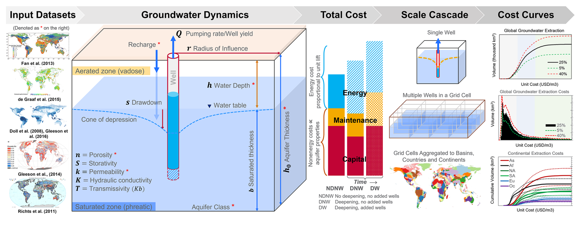
Figure 1Conceptual overview of Superwell including input hydrogeologic datasets; a single example grid cell with a pumping well showing aquifer properties, pumping target, and groundwater dynamics captured in the model, along with model features such as well deepening and replacement; cost accounting components and their variations with model dynamics; scale cascade feature allowing spatial flexibility in cost aggregation; and example cost curves as an illustrative output of Superwell across stylized scenarios described later.
Cost curves are generated within the control volumes of individual grid cells assumed to have homogeneous hydrogeological properties (depth to water, porosity, aquifer thickness, and hydraulic conductivity). The control volumes define the parameters used by the Theis analytical solution (Theis, 1935) to represent the transient aquifer pressure response from a pumping well. Groundwater storage and aquifer properties (depth to water, saturated thickness, and transmissivity) for each grid cell are updated annually due to recharge or as aquifers are depleted due to pumping (Fig. 1). Superwell iterates over each gridded control volume within a spatial area of interest (here, the entire globe) and simulates groundwater pumping and associated costs (described in detail below) to produce grid-cell-specific cost curves. The derived cost curves generated by Superwell can then be integrated with economic models that represent water use behavior (Niazi et al., 2024c; Turner et al., 2019b; Hejazi et al., 2023) (Fig. 1).
The cost curve approach employed in Superwell represents fully spatially developed groundwater production in each grid cell control volume where the entire cell surface area is occupied by service areas for hypothetical pumping wells (scale cascade in Fig. 1), each producing groundwater for a defined service area. This assumption is reasonable given the time-independent nature of cost curves, which only define cumulative production and unit cost. In theory, without recharge, a cost curve for a grid cell could be produced by simulating a single well pumping for tens of thousands of years, and the resulting cost curve would be mostly equivalent to the same grid cell having thousands of wells that are pumped for only a few hundred years. Thus, the full spatial coverage does not represent existing wells but rather is used to approximate the cost to extract each new unit of groundwater for a given grid cell without having to run extremely long simulations. Conversely, with recharge, the depth to groundwater changes annually based on recharge, but the annual pumping target remains constant within a year after accounting for shallow recharge, which makes the approach to determining well area from pumping rates still applicable. Adding recharge influences depletion and demand in two ways. First, recharge reduces the depletion rate due to pumping by reducing the net depletion in each annual time step. Second, it also reduces the annual pumping target because we allow a specified fraction of recharge to reduce the annual pumped volume target, which coarsely represents recharge satisfying some amount of irrigation requirements. The area served by each well is homogeneous within each grid cell (illustrated as radius of influence in Fig. 1) and determines the total number of wells in a grid cell. The area served is determined by the well pumping rate for the grid cell and a user-defined annual ponded depth requirement (which may vary endogenously by the recharge rate as described in detail in Sect. 2.2.3). Additional external factors like water governance or the cost of transportation and treatment are not considered.
This generalizable methodology is primarily driven by aquifer properties, recharge and extraction scenarios to describe scale-specific boundary and initial conditions, and therefore could be tailored to custom applications depending on locations and scales of interest. For instance, we present a global-scale application of Superwell at 0.5° resolution parameterized using global gridded datasets of subsurface properties (Fig. 2). We also explore the effect of different annual ponded depth requirements and groundwater depletion limits on extraction costs. The annual ponded depth target ensures that the cost curves reflect well attributes (pumping rate, well spacing) capable of producing reasonable annual volumes for groundwater use, even though the cost curves themselves are time agnostic. The well capacity–area approach employed in Superwell was informed by empirical relationships between well capacity and irrigated area documented by Foster et al. (2015), who showed a strong relationship between well capacity (pumping rate) and irrigated area. The bounding annual ponded depth target can be chosen by the user if unit cost implications of higher (or lower) ponded depths are of interest (but net ponded depth targets are determined in the model using recharge rates).
2.1 Global hydrogeologic input data
Global hydrogeologic data are sourced from publicly available datasets that include depth to groundwater (Fan et al., 2013), aquifer porosity and permeability (Gleeson et al., 2014), aquifer thickness (de Graaf et al., 2015), long-term annual averaged recharge rates (Döll and Fiedler, 2008; Gleeson et al., 2016), aquifer classification (Richts et al., 2011), and inland lakes (Messager et al., 2016). The datasets were geo-processed to produce a vector dataset that defines the mean hydrogeological properties and aquifer classes over a 0.5° (≈50 km × 50 km) grid at the coarsest resolution as shown in Fig. 2 (aquifer classification from Richts et al., 2011, is shown in Fig. S1 in the Supplement). Aquifer porosity and permeability data were upscaled to the 0.5° resolution by using mean values within a grid cell, and recharge rates and lakes were regridded using an area weighting. Some limitations of the global hydrogeological datasets have been mentioned in the Supplement. Due to the irregular geometry of political boundaries (country borders), geographic boundaries (basins, coastlines), and aquifer classification, the resulting processed global geospatial data are not a uniform rectilinear grid and instead capture the area where land surface boundaries intersect with gridded hydrogeological data. The processed global dataset has a total of 106 439 grid cells that serve as inputs for Superwell (Niazi et al., 2024b). The model design has been kept flexible to the source of the input datasets, so any improvements in the quality or resolution of hydrogeological input datasets could be incorporated as updated inputs to the model.
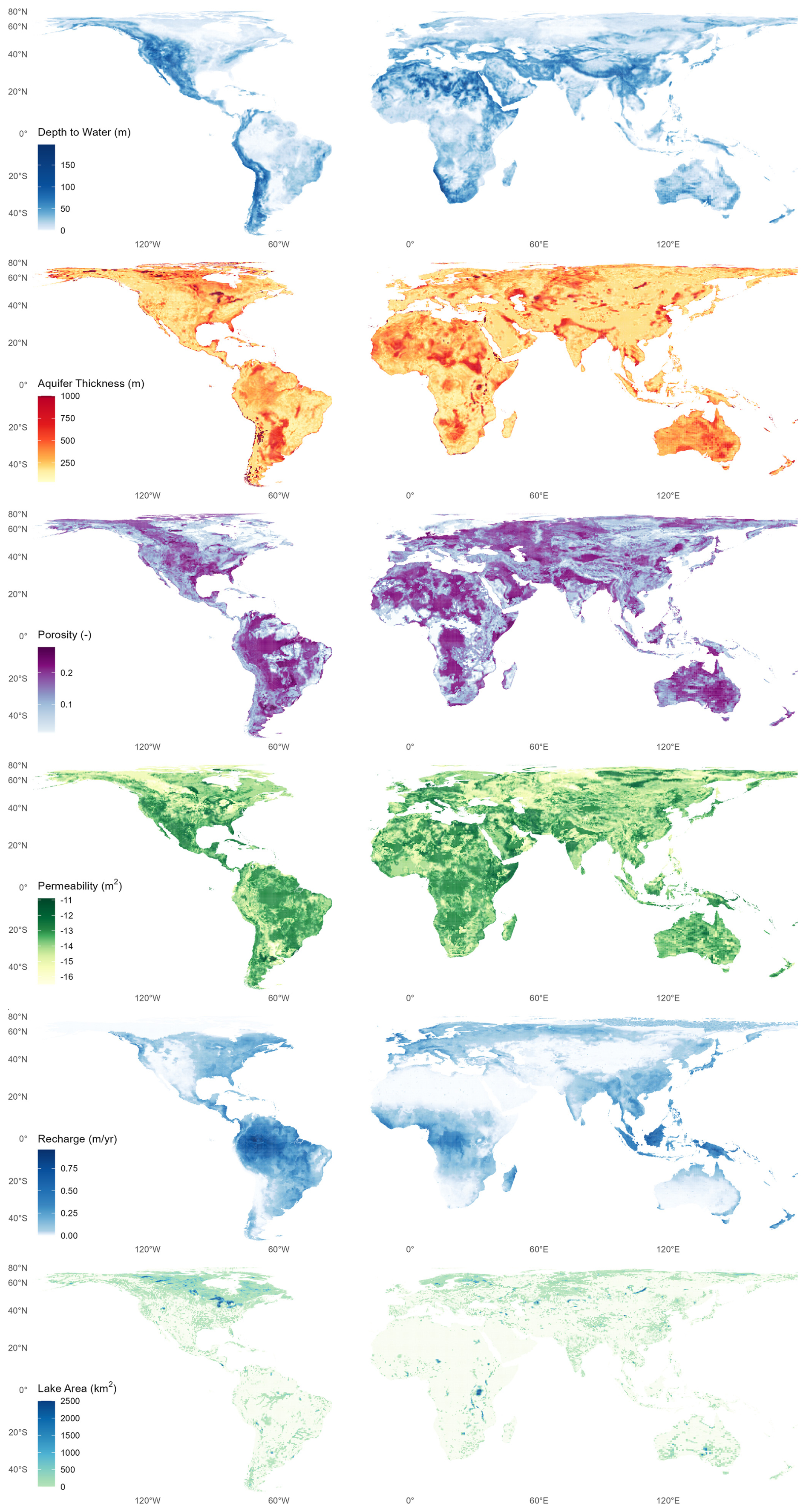
Figure 2Global hydrogeologic datasets digitized to evaluate groundwater availability and serve as inputs to Superwell (Niazi et al., 2024b): depth to groundwater (Fan et al., 2013), aquifer thickness (de Graaf et al., 2015), porosity and permeability (Gleeson et al., 2014), recharge (Döll and Fiedler, 2008; Gleeson et al., 2016), and lakes (Messager et al., 2016).
2.2 Model design – overview of Superwell algorithm
A step-by-step summary of the Superwell algorithm is presented in Fig. 3 and Algorithm A1 (Niazi et al., 2025). The workflow illustrated in the wire diagram is executed for each grid cell in the input dataset. The first step is to screen whether groundwater production is feasible given the defined hydrogeological properties. If a grid cell meets the initial screening criteria, the algorithm advances to the “pumping phase” that simulates well pumping and resulting aquifer depletion, followed by a “cost phase” that calculates the cost of groundwater production (Fig. 3). These pumping and cost phases are executed sequentially (in series). This section describes the high-level structure of the Superwell algorithm, whereas detailed descriptions of the methodological assumptions and underlying equations are presented in the following subsections.
The screening criteria for determining whether a grid cell progresses to the pumping phase are based on a set of specific thresholds and conditions. First, we apply screening based on the fraction of grid cell area covered by lakes (considering lakes larger than 1 km2), as defined by the HydroLAKES global dataset (Messager et al., 2016). We skip the grid cells where lakes cover more than 95 % of the grid cell area. For simulated cells, where the lake area is less than 95 % of the grid area, we calculate the dry area (grid area − lake area) to be used for the rest of the calculations. In addition, grid cells with an area less than 5×5 km2, representing 1 % of the standard 50×50 km2 grid size, are excluded to omit abnormal intersections of rectilinear grid, geographical boundaries and classification of aquifers. Grid cells with permeability values lower than 10−15 m2 are not considered for pumping due to their limited ability to transmit water. Cells with less than 5 % porosity are also skipped to avoid cells with low water storage capacity. To ensure pumping from a realistic depth, any outlier aquifer thickness exceeding 1000 m is adjusted to this maximum value. Finally, grid cells where the depth to the water table is greater than the aquifer thickness are skipped, as this results in negative transmissivity, rendering groundwater extraction infeasible.
The pumping phase starts with the selection of an initial pumping rate for the wells in a grid cell. Pumping rate can have a strong influence on unit groundwater cost, and the procedure for determining well pumping rate is described in Sect. 2.2.3. If the aquifer cannot support a pumping rate of at least 0.00063 m3 s−1 (or 10 gallons per minute, gpm) without exceeding the drawdown criteria which establishes the maximum allowable total or fractional drawdown at the well (Sect. 2.2.3), the pumping phase terminates, the grid cell is skipped, and the algorithm moves to the next grid cell. If the aquifer can support a pumping rate above 0.00063 m3 s−1, the model then initiates the annual pumping loop where groundwater pumping occurs for user-specified days each year (100 d for the current implementation). The 100 d assumption is based on upper bounds for annual average days of irrigation well pumping from US Department of Agriculture Farm and Ranch Irrigation Survey data (USDA, 2024). Bierkens et al. (2022) also assume 100 d of pumping for their global analysis of groundwater use for irrigation. Additionally, domestic wells or wells used for municipal supply are typically not operated 24 h a day, 7 d a week, making it a reasonable assumption to represent pumping for ∼30 % of the hours of the year (see Supplement for details). As aquifer saturated thickness decreases due to depletion, the ability of the aquifer to support a given well pumping rate decreases. This first manifests in a larger drawdown at the well head for the same pumping rate (which increases pumping cost), but eventually the drawdown at the well can exceed the remaining aquifer thickness, leading to dewatering of the well. To prevent dewatering from occurring, during each annual period (t=y), with the exception of the first year (t=1), the pumping rate from the previous year () is used to forecast drawdown during the upcoming 100 d pumping period to check if the aquifer will be able to support the current pumping rate. If it cannot, the pumping rate is reduced, and the current annual period (t=y) is simulated; otherwise, the pumping rate from is used.
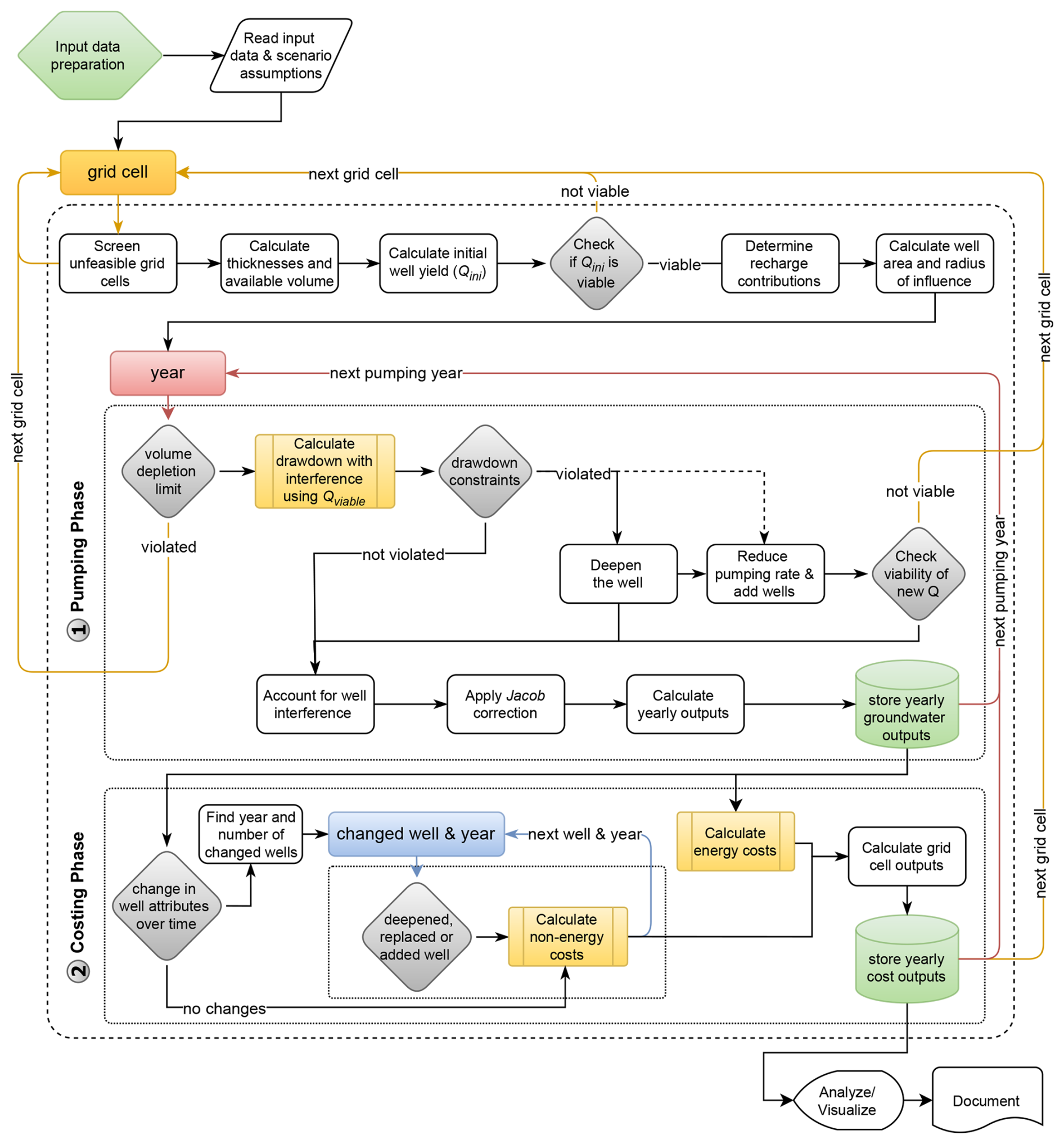
Figure 3Superwell workflow diagram illustrating going from global gridded data to grid cell and regional cost curves that can serve as input to an economic model of water use (e.g., GCAM) (Niazi et al., 2025). Dotted boxes demarcate major containerized phases in the model simulation. Boxes represent key steps in the workflow; diamonds control key conditionals; and colored lines represent key loops for iterations over grid cells, pumping years, and cost accounting.
There is also a default well-deepening functionality that can dynamically deepen wells (increase aquifer capacity) to maintain the initial pumping rate. If this feature is used, the pumping rate is not decreased until the well has been deepened to the maximum aquifer depth. If well deepening is not used, wells start at the total aquifer depth, as defined by de Graaf et al. (2015). At the end of each annual period, outputs are saved to arrays to track annual changes to aquifer properties (water depth, saturated thickness, transmissivity) and well properties (pumping rate, well depth, drawdown during pumping) that are used for the next annual pumping period and also for annual cost calculations.
The number of years of pumping in the pumping phase is controlled by two user-specified parameters: simulation length and depletion limit. The simulation length is the maximum possible pumping duration (in years), while the depletion limit is the maximum allowable aquifer depletion, expressed as a fractional decimal value (i.e., 0.25=25 %). The pumping phase for a given cell is terminated if the model reaches the maximum number of annual time steps or if the ratio of pumped groundwater volume to initial available volume exceeds the depletion limit. For this paper, the total simulation period has been set to a long enough period (500 years) so the majority of grid cells reach the depletion limits defined by depletion limit scenarios we consider (Sect. 2.3). Total pumping duration can impact grid cells differently; for example, for hypothetical settings where the simulation length is 100 years and the depletion limit is 0.5, a thick aquifer would be pumped for the entire 100-year period, while a thin aquifer with low storage would reach the depletion limit before the end of the 100-year period, at which point pumping would stop. After the pumping phase has ended, annual cost components are calculated in the cost phase using outputs from the pumping phase. Annual costs include capital, maintenance, and energy costs of pumping (described in sections under Sect. 2.2.4).
2.2.1 Modeling well hydraulics
The aquifer response to pumping is simulated using the Theis analytical solution (Theis, 1935) for the transient aquifer pressure response due to a pumping well (Eq. 2). In order to use the Theis solution, permeability values (k in m2 units) are converted to hydraulic conductivity (K) using assumed values of water density (ρ), gravitational acceleration (g in m s−2), and dynamic viscosity (μ) at 20 °C (Eq. 1).
Saturated thickness (b) is defined by the difference between well depth and water depth in the time step being modeled, , and aquifer transmissivity (T in m2 s−1 units) is calculated as a product of hydraulic conductivity and saturated thickness (T=Kb). (Note that the definition of b may be slightly different from the conventional definition used for confined aquifers (depth from the water table to the bottom of the confining unit).) Aquifer transmissivity and storativity along with well pumping rate are used in the analytical Theis solution to calculate drawdown in Eq. (2), which assumes homogeneous, isotropic aquifer properties (storage, hydraulic conductivity, and saturated thickness). Laterally, we assume no-flow boundaries between grid cells. Groundwater head recovery during the non-pumping period was not simulated – e.g., by using superposition in time to represent recovery by simulating an equivalent injection rate after 100 d. We assume that the cone of depression around each well created during the 100 d of pumping mostly re-equilibrates to an initial, horizontal state (minus the volume depleted) during the non-pumping period of the year (265 d of no pumping), which is a reasonable assumption given the 100 d pumping period considered in this study (see more details in the Supplement). The Theis approach, as presented in Eq. (2), describes the pressure response to pumping at any time since pumping began and at any distance from the pumping location.
where s is drawdown (m), Q is well pumping rate or well yield (m3 s−1), T is the aquifer transmissivity (m2 s−1), and W(u) is the well function. The well function W(u) in the analytical solution of Theis Eq. (2) is an exponential integral Ei and for small values of u can be approximated by the infinite series in Eq. (3).
where u is defined by Eq. (4).
where r is the radial distance from pumping source (m), S is aquifer storativity assumed to be equal to aquifer porosity in this study (–), T is aquifer transmissivity (m2 s−1), and t is the time since pumping started. Uniform length and time units must be used for Theis Eqs. (2) and (4) for u. The value of W(u) in Superwell is determined using a conditional statement based on the u value. For very large u values, representing either early time or large r, the well function is set to zero W(u)=0; for intermediate values of u, the well function is determined from a lookup table u:W(u) whose values are sourced from Brown et al. (1964); and for small values of u, W(u) is approximated by the first four terms of Eq. (3).
A radial distance of 0.28 m, representing negligible well diameter, is used to determine transient drawdown at the well head that is used for determining the pumping cost and pumping rate feasibility. Drawdown is calculated at 10 d increments, and the average drawdown over the 100 d period is used for pumping cost calculations. To account for the well interference of adjacent wells on the drawdown of a central well, we calculate the distance to adjacent wells (radjacent) using the well area of the central well (Awell) in Eq. (5) and determine the additional drawdown they contribute.
Drawdown for adjacent wells (sadjacent) is calculated at radjacent, and then additional drawdown due to adjacent wells is added to the drawdown of the pumping well () to account for the additional drawdown due to well interference. The user can specify the number of adjacent wells – i.e., four wells indicate square packing and six wells indicate circular packing; the results here assume circular packing of wells. Notably, the range of well spacings, pumping rates, and the pumping period of 100 d result in marginal additional drawdown but are accounted for completeness. Thus, the total pumping lift (hlift in Eq. 6) used for calculating the energy cost of pumping is the sum of the average drawdown at the well (swell), the additional drawdown from the nearest wells, and the depth to water (hwater) before pumping starts.
A notable limitation of the Theis analytical solution is the assumption that saturated thickness remains constant during pumping, which is only applicable to confined aquifers. For our application, we represent pumping in unconfined aquifers (also called phreatic) where the saturated thickness changes in response to pumping. The Jacob approximation (Jacob, 1947; Brown et al., 1964) provides a means to use the Theis result to calculate the equivalent drawdown in an unconfined aquifer (Eq. 7).
where su is the drawdown in the unconfined aquifer (in this case the drawdown at the well with interference), sc is the drawdown in a confined aquifer from Eq. (2), and b is the saturated thickness. Drawdown in unconfined aquifers (su) can be calculated by solving the quadratic equation , where , beq=1, and from Eq. (7). Superwell first calculates the drawdown for a confined aquifer and then converts it to an equivalent drawdown for an unconfined aquifer using Eq. (7).
Pumping during each annual period is simulated as 100 d of pumping in each year, similar to Reinecke et al. (2023), followed by 265 d of recovery. The choice of a constant pumping period followed by an off period was a compromise between approximating representative well operations, computational efficiency, and reasonable annual total groundwater production volumes per well. Groundwater wells are seldom operated continuously on long yearly scales. Instead, wells are used intermittently to provide supply to end uses such as irrigation, industrial operations, or municipal water supply. Since groundwater is predominantly used for agriculture, 100 d periods reasonably approximate the seasonality associated with crop production, while also producing reasonable unit cost estimates for other applications such as industrial or municipal use. Besides being unrealistic, constant pumping could also underestimate unit costs as the total pumped volume to well cost ratio would be inflated by year-round operation.
2.2.2 Incorporating recharge
Recharge rates are important in determining pumping requirements and groundwater storage levels for a region. We take gridded long-term annual averaged recharge rates from Döll and Fiedler (2008) and Gleeson et al. (2016, 2012), regrid them to match Superwell's grid using an area-weighted approach, and adjust the ponded depth targets and depth to groundwater based on recharge rates. We implement the effect of recharge in two ways: (1) to incorporate the response in shallow subsurface that potentially reduces the pumping requirement (currently set to 20 % of total recharge) and (2) in deep storage that increases groundwater stocks on longer timescales to potentially reduce depth to groundwater. The relative contribution to shallower parts compared to deeper parts of the aquifer can be controlled by the user, where recharge rates determine the magnitudes of ponded depth target reduction and depth to groundwater reduction. User-controlled checks have been put in place to prevent fully eliminating the ponded depth target from shallow recharge contributions (such as a threshold depth ratio of 0.75, making the ponded depth target never fall below 75 % of its original value due to shallow recharge adjustment). Although never activated in the current default settings, the processing also allows passing on “leftover” shallow recharge (not used to reduce ponded depth target) to deep groundwater storage to maintain recharge accounting. However, recharge contributions to deep parts of the aquifer do not exceed annual pumping volumes (avoiding groundwater accumulation) to ensure cost accounting for each simulated grid cell. Including recharge dynamics into Superwell enables accounting for the impacts of varying contributions to groundwater from the surface on pumping dynamics and cost accounting, including under alternative climate change impact scenarios. Varying sub-annual, gridded groundwater costs under climate impacts, as enabled by the incorporation of recharge components (that alter the pumping requirements and deep aquifer storage level), could be a valuable resource for hydro-economic models and studies exploring groundwater's role in enabling water and food security globally.
2.2.3 Determining well pumping rate
Well pumping rate and recharge-adjusted ponded depth target determine the well area, which has important unit cost implications. Well area, in combination with grid cell area, determines the number of wells in a grid cell and the subsequent capital and maintenance cost requirements which share a significant portion of total and unit costs of supplying groundwater (Fig. 8). The initial pumping rate is determined from a range of candidate pumping rates spanning from 10 to 1500 gallons per minute (or 0.00063 to 0.09463 m3 s−1). The upper bound is informed by the typical upper range for irrigation wells (USDA, 2024), while the lower bound represents a practical lower end for irrigation and other applications, beyond which very high, uneconomical unit costs were observed. The range of candidate pumping rates is used to perform an iterative evaluation of all candidate rates whenever the well pumping rate needs to be determined. This evaluation happens both during the selection of an initial pumping rate in the first year of the pumping phase and when the pumping rate needs to be reduced to prevent well dewatering, if the current pumping rate exceeds the aquifer capacity.
Wells are installed under an assumption to have high but reasonably sustainable pumping rates. Here, sustainable means that the initial pumping rate will be viable for more than just a few years. Candidate pumping rates are screened by simulating drawdown for 2 years of constant pumping. Total drawdown and drawdown fractions (ratio of drawdown to screened aquifer saturated thickness) are then calculated at t=2 years for all candidate pumping rates. A hard limit of 80 m is used for the absolute drawdown, and 0.4 is used for the maximum drawdown fraction that limits the drawdown to 40 % of saturated aquifer thickness. Pumping rates must satisfy both drawdown criteria to be considered viable. The largest viable pumping rate is used to establish the initial pumping rate which drives pumping over years until it can no longer satisfy the drawdown criteria. A new viable pumping rate is determined in subsequent years when the pumping rate needs to be reduced due to aquifer depletion. The reduced pumping rate also reduces the well area, which in turn adds more wells in the same grid cell. This increases infrastructure costs due to installation of new wells while reducing energy costs per well due to the reduced pumping rate. The pumping phase terminates if the lowest pumping rate is not viable.
2.2.4 Hydro-economics
One of the key contributions of Superwell is tracking energy and non-energy costs of pumping groundwater emerging from well characteristics and volumes pumped under hydrogeological controls. These controls include grid-specific hydrogeological conditions, aquifer properties, well hydraulics, and decision constraints of pumping regimes that emerge from user-defined pumping scenarios. This section describes energy, capital, and maintenance cost calculations, along with unit cost calculation under model controls, constraints, and scenarios.
Cost accounting formulation
The cost phase uses well attributes and pumping phase outputs to calculate the total cost of groundwater extraction and eventually the unit costs of pumping. The total cost for each year of pumping is the sum of the annual energy, capital, and maintenance costs (Eq. 8):
Pumping cost (Eq. 9) is defined by the total energy (kilowatt hours, kW h) required to pump the annual volume of groundwater from a grid cell multiplied by the country-specific energy cost rate for electricity (er, USD 2016 kW h−1) sourced from IEA (2016).
The energy required to pump groundwater is calculated using Eq. (10).
where ρw is the specific weight of water (assumed to be 9800 kg m−3); Hyr is the distance (m) that water has to be lifted during pumping in a given year and is the sum of the water depth (hwater,yr) plus the average total corrected drawdown (savg,yr); Qyr is the pumping rate in the given year; tpumping is the 100 d pumping period in hours (2400 h); and η is the well efficiency, assumed to be 0.7.
Capital cost associated with the installation of the well is represented by an amortization-based cost accounting approach that estimates annual payments on a loan issued over the well lifetime using Eq. (11).
where i is the interest rate on the loan assumed to be 0.1, n is the loan duration currently equal to the well lifetime to distribute loan payments over the lifetime of a well, and Cinstall is the installation cost defined by Eq. (12).
where well unit cost (cu,aquiferClass, USD m−1) is a function of the WHYMAP aquifer classification (Richts et al., 2011) and the hwell,yr is the well depth in a given year. The well unit cost has three values reflecting costs of installing a well in easy (USD 50 m−1), normal (USD 82 m−1), and complex (USD 164 m−1) aquifers. Well depth unit costs are sourced from Advisor (2018). Annual maintenance costs are calculated based on the current installation cost (i.e., well depth) with an annual assumed fraction of 7 % () to represent increasing maintenance costs for deeper wells. A few examples of maintenance costs are pump maintenance or replacement, flushing of fines from the well to maintain pumping capacity, and descaling of precipitates from the well screen (Glotfelty, 2019).
Additional steps are required to calculate the evolution of annual infrastructure costs when wells are deepened or their pumping rates are reduced to prevent violation of the drawdown thresholds (Sect. 2.2.3). The cost phase tracks annual costs associated with wells as they are added and deepened. Increased costs from deepening wells are represented by an amortized loan over the well lifetime (20 years) for the additional depth added. During the time step of deepening, these costs are added to the next n years, currently set to a well lifetime of 20 years. If the well pumping rate must be reduced to prevent exceedance of the drawdown limit, the number of wells in the grid cell is increased to compensate for the reduced production per well. The cost array tracks each new addition of wells from their own reference time, and those wells are replaced at the end of each well's lifetime (n) interval. If they are deepened, the additional cost is applied as a loan for that specific group of wells over the lifetime of the well.
Unit cost evaluation
Unit costs are calculated to express the economic burden of groundwater extraction capacity by taking into account both extraction volumes and their associated costs. Unit cost of pumping groundwater is the ratio of the total cost incurred for pumping groundwater and the total volume pumped within a grid cell in each year. Total costs of pumping from a well (Ctotal,yr) is multiplied by the number of wells in a grid cell (nwells) to obtain total annual costs of pumping groundwater from all wells within a grid cell for each pumping year (CGW,yr). This is shown in Eq. (8).
The number of wells is determined by the area of the grid cell divided by the area served by one well (), where area served by a well is estimated by well yield (Q), pumping duration in a year (pumping days converted to seconds), and ponded depth target (dp) as shown in Eq. 14.
The total volume pumped by each well is based on the annual well yield multiplied by the duration of pumping in a year (number of pumping days in a year). The total volume pumped by all wells is then the product of the volume pumped per well and the number of wells.
The unit cost of producing groundwater is a key attribute of cost curves. Unit cost (cunit) is calculated as a fraction of total cost incurred by pumping groundwater and total volume pumped within a grid cell in each year as shown in Eq. (16).
The unit cost relation in Eq. (16) is also applicable to other spatial and temporal scales; for example, unit costs could also be calculated for basins on a decadal pumping scale. Superwell currently calculates unit costs on a finer resolution (annually for each 0.5° grid cell), which could be upscaled later in post-processing using the spatial mappings (grid, basin, country, region, continent) provided with the model.
2.3 Scenarios
A global demonstration of Superwell is presented by subjecting each grid cell to six scenarios of groundwater extraction to capture various limits to total groundwater production. Two annual ponded depth targets of 0.3 and 0.6 m (which may reduce endogenously in the model due to recharge) and three global groundwater depletion limits of low (≤5 %), moderate (≤25 %), and high (≤40 %) aquifer volume depletion were used to create six scenarios for evaluating groundwater pumping regimes and unit costs over the extraction lifetime. Ponded depth targets represent a depth of groundwater spread over a land surface area that might have a variety of sectoral uses. It constrains the well area such that the depth resulting from spreading annual volume pumped by a well over the well area equals the ponded depth target. Groundwater depletion limits represent the allowable volume fraction of the total available groundwater that can be pumped at each grid cell – e.g., a depletion limit of 25 % means that pumping can continue until the remaining storage is 75 % of initial storage in each grid cell. The three limits selected for this demonstration are intended to represent a range of plausible depletion criteria.
In practice, aquifer depletion criteria are often employed to protect regional economic, social, and environmental interests (Korus and Burbach, 2009). The selected limits may seem conservative in comparison to levels of observed aquifer depletion – for example, while total storage for the Ogallala aquifer was only 30 % depleted in 2010 (Steward et al., 2013), localized depletion has surpassed 75 % in some parts of the aquifer where there has been extensive and long-term groundwater use (McGuire and Strauch, 2024). In reality, depletion limits will be highly site-specific and adapted over time due to changing interests; however, the three limits selected are meant to illustrate generalized scenarios bounding a range of potential depletion criteria (Korus and Burbach, 2009; Sophocleous, 2000; McGuire et al., 2003).
3.1 Model evaluation approach
Superwell's simulations extend until reaching the user-defined depletion limits of groundwater reserves, facilitating a comprehensive exploration of volume-to-cost combinations. Pumping volumes and related parameters (e.g., pumping rate, number of wells in a grid cell) simulated in a scenario are not meant to be interpreted as representations of real-world aquifer pumping. Instead, they represent a plausible range of pumping conditions an aquifer might encounter until it is exhausted. This modeling philosophy aimed at sketching out the possibility space for groundwater extraction and its cost implications globally makes conventional observation-based validation of the model unfeasible. Instead, an expert-centric evaluative approach has been employed, which qualitatively confirms the model's behavior to be consistent with expected trends and patterns in groundwater pumping dynamics and their cost implications (Gleeson et al., 2021).
3.2 Influence of hydrogeologic properties on well attributes and cost components
A novel advancement of Superwell is accounting for the control of hydrogeologic properties on maximum well pumping rates, which in turn affects groundwater cost components (energy cost, non-energy cost, and unit cost). We have curated a series of diagnostics (Fig. 4) directly from Superwell under the moderate-depletion scenario (≤25 % aquifer depletion and 0.3 initial ponded depth target) using grid cells within the United States (n=3769 cells) as an example to illustrate key relationships between aquifer properties (inputs) and resulting well attribute (e.g., depth, pumping rate) and cost outputs. In the following sections, we use Fig. 4 to describe key patterns demonstrating the influence of hydrogeologic properties on well attributes and cost components.
3.2.1 Diagnostics for well hydraulics
Figure 4a highlights the relationship between aquifer properties and well yield (also referred to as pumping rate). Hydraulic conductivity (K) and transmissivity (T) exhibit a direct relation with well yield, confirming that aquifers with both higher hydraulic conductivity and greater saturated thickness can support higher pumping rates, agreeing with well theory (Theis, 1935). As noted by the Theis Eq. (2), transmissivity and storativity (reflective of porosity) determine the drawdown response of a well at a given pumping rate. Consequently, when storativity remains constant, aquifers characterized by higher saturated thickness and hydraulic conductivity can support higher pumping rates compared to thinner and lower-conductivity aquifers.
Well yield and well area have a direct relationship in Superwell varied by annual pumping requirement as a result of varying ponded depth targets due to recharge (Fig. 4b). This relationship implies that as the well yield decreases, well area decreases, with smaller well areas for larger ponded depth targets. Reduced well yield results in an increase in number of wells in a grid cell and an increase in unit capital cost due to the need for more wells. Note that well yield and well area are variable and subject to change over time due to aquifer depletion or management strategies that aim to reduce depletion. As aquifer storage declines due to pumping (i.e., depletion), well yield is adjusted accordingly to meet the dynamic conditions and well area is adjusted to achieve the net ponded depth target.
Figure 4c shows a relation between transmissivity (T=Kb) and Jacob-corrected drawdown for unconfined aquifers at the well head for a range of well yields. This figure reinforces the relation in Fig. 4a that higher transmissivity allows for higher well yields and vice versa. Further, as transmissivity decreases over time due to a reduction in aquifer saturated thickness, the drawdown for a given well yield increases as lower transmissivity results in more drawdown near the well to extract the same quantity of water. This explains the indirect and nonlinear relation between decreasing transmissivity and increasing drawdown. Figure 4c also reflects our assumption that drawdown cannot exceed the absolute drawdown threshold of 80 m. Notably, the screening process of selecting viable well yield is designed to select initial drawdowns closer to the upper limit of 80 m or 40 % of initial saturated thickness to maximize well yields initially. The fractional drawdown limit of 40 % means some locations could become non-viable with drawdowns below the 80 m absolute drawdown limit if the drawdown of those wells under the lowest pumping rate of 0.00063 m3 s−1 is more than 40 % of the aquifer's current saturated thickness.
3.2.2 Diagnostics for cost dynamics
Unit costs (USD m−3) are observed to be higher at lower well yields and greater water depths (Fig. 4d). Non-energy costs per unit groundwater pumped are higher for wells that produce less volume, resulting in changes to observed unit costs. For example, for two wells of the same depth (i.e., having identical non-energy costs per well) in aquifers that support different well yields, the well in the lower capacity aquifer would have a higher unit cost because the non-energy cost per unit groundwater pumped would be higher. At the grid cell scale, lower yield wells also have smaller areas served (Fig. 4b), which results in a greater number of wells (and thus higher non-energy cost). Larger water depths also increase unit costs and total cost per well due to the higher energy costs needed to lift a unit of groundwater.
Assuming the number of wells remains constant, larger water depths require more energy to extract a certain volume of groundwater, leading to higher annual energy costs per well (Fig. 4e). Higher well yields also result in higher energy costs per well as more volume is extracted over the annual pumping period. Both of these relationships, as shown in Fig. 4e, can be explained by Eq. (10).
Figure 4f shows that non-energy costs (capital and maintenance) are dependent on well depth and aquifer class, which represent the ease of installing a well and its associated costs. The interest rate for amortization of installation costs, maintenance costs, and well lifetime affect the non-energy costs but are kept fixed for this documentation. This panel also shows increasing non-energy costs with increasing well length (where the “tuning-fork” like separation is due to the well-deepening feature of the model). The deepest wells in the most complex hydrogeological conditions have the highest non-energy costs.
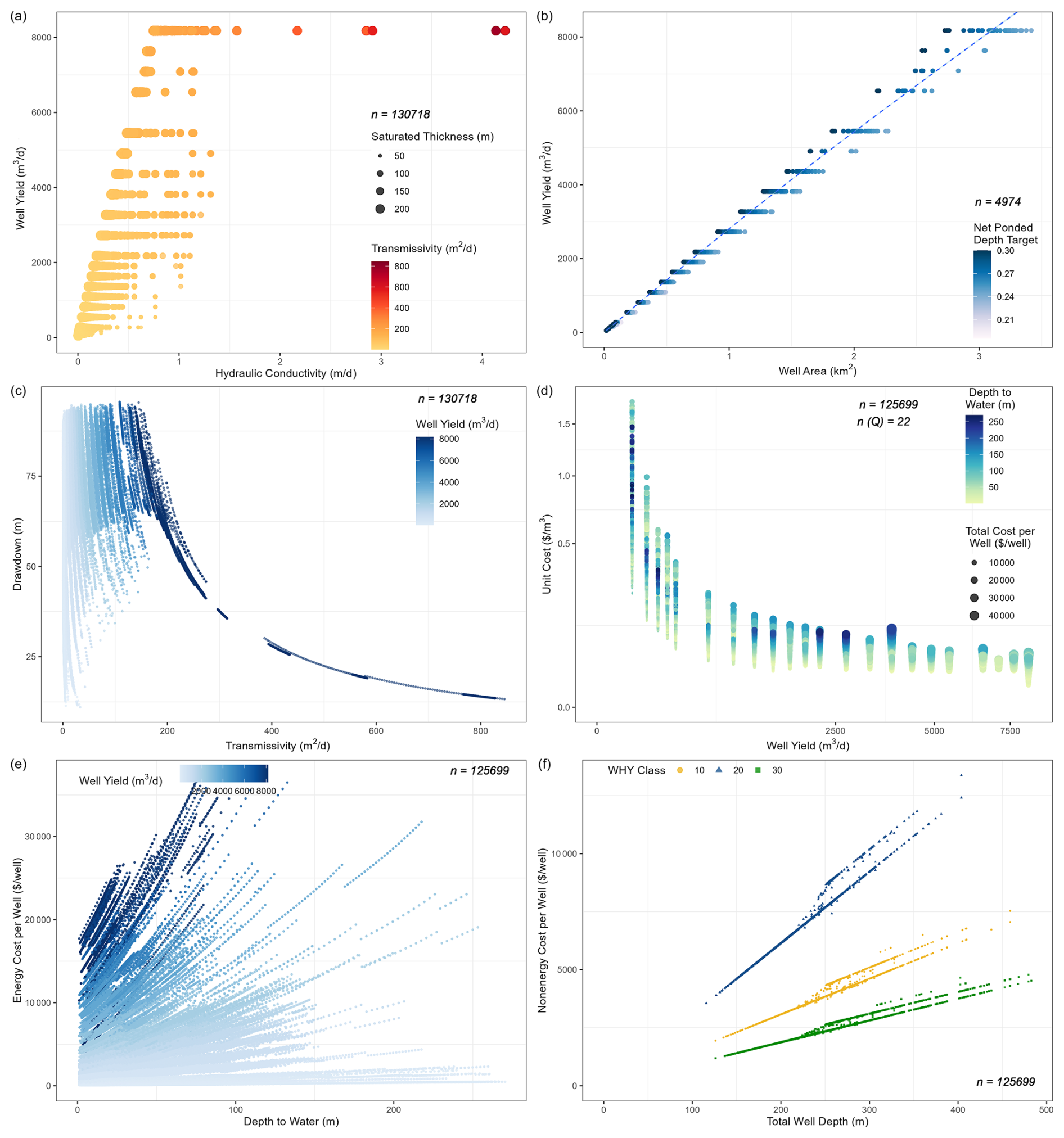
Figure 4Key diagnostics curated to demonstrate patterns in model behavior emerging as a result of the influence of hydrogeologic controls and aquifer properties on well attributes and cost components using the United States as an illustrative example. n in each panel represents the number of unique data points within all US grid cells (3769) during all years of pumping (changes for each grid cell).
Superwell produces an array of outputs (more than 20 primary variables) that provide insights into the dynamics of groundwater pumping and associated costs (Niazi et al., 2024a). The results presented here focus on a select subset of the outputs, including estimates of globally available groundwater, physically and economically extractable volume, and their energy and non-energy costs, along with unit costs and its relation with cumulative groundwater production to provide spatially flexible cost curves of the groundwater supply (Niazi et al., 2024a). All global maps presented as results depict the moderate-depletion scenario targeting 0.3 m of ponded depth and allowing 25 % of aquifer volume depletion.
4.1 Volume assessment
4.1.1 Initial global groundwater availability
The challenge in building global groundwater extraction unit cost curves is partly attributed to characterizing aquifers that are economically, hydrogeologically, and environmentally feasible for production. Before showcasing Superwell results about groundwater extraction and associated costs, our processing of input datasets suggests that 5.22×10⁶ km3 of groundwater is initially available in storage globally. Here, available groundwater, estimated using Eq. (17), refers to the amount of water present in storage, not necessarily what is feasible or practical to produce. Estimating the initial groundwater availability aids in setting an absolute upper bound to the volume available for pumping in each grid cell. Figure 5 shows this availability expressed as ponded depth by normalizing available volume with grid cell area (). This normalization removes the influence of grid cell area on the volume calculation and shows groundwater availability as if it was extracted and pooled on the land surface directly above storage.
where Vavailable is the global available groundwater volume (m3), i is each grid cell in all grid cells E, b is saturated thickness (aquifer thickness − depth to water, m), Agrid is areal extent of grid cell (m2), ϕ is porosity, and dp is the ponded depth of groundwater (m).
The initial groundwater availability exhibits considerable spatial heterogeneity stemming from the underlying hydrogeological properties. The ponded depth of available groundwater in Fig. 5 shows that regions with thick aquifers and high porosity (Fig. 2) are associated with higher groundwater availability. Higher ponded depths are observed across a wide range of hydroclimates spanning from tropical (Amazon) to arid regions (Sahara, central Australia), suggesting a stronger hydrogeologic control than climate on total groundwater in storage. Similarly, regions with low ponded depths do not strictly coincide with arid regions. For example, the Congo and southern India show low storage despite having high annual precipitation. Instead, low storage is more closely associated with thinner aquifers with low porosity.
Estimates of total groundwater storage are highly uncertain due to lack of hydrogeological data at a global scale (Reinecke et al., 2023), with quantifications varying by over an order of magnitude (1 to 60×106 km3) depending on the methodology followed (Nace, 1969, 1971; Garmonov et al., 1974; L'vovich, 1979; NRC, 1986; Gleeson et al., 2016); see Table A1. While our estimate falls within the range noted in the literature, it is highly conditional on the input datasets described earlier. Despite uncertain estimates of aquifer properties and global groundwater availability, calculating available groundwater from the best-available data sources still offers some value. In the absence of such an estimate, modelers of integrated water–energy–land dynamics would have no credible means to limit groundwater depletion from storage (Kim et al., 2016; Vinca et al., 2020).
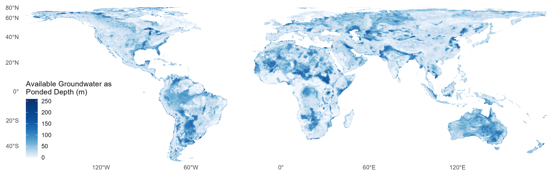
Figure 5Global groundwater availability presented as ponded depth (i.e., volume available dived by grid cell area). While it is not used in Superwell simulations, it gives a sense of how much groundwater is initially in storage according to input datasets in Fig. 2.
4.1.2 Pumped groundwater volume
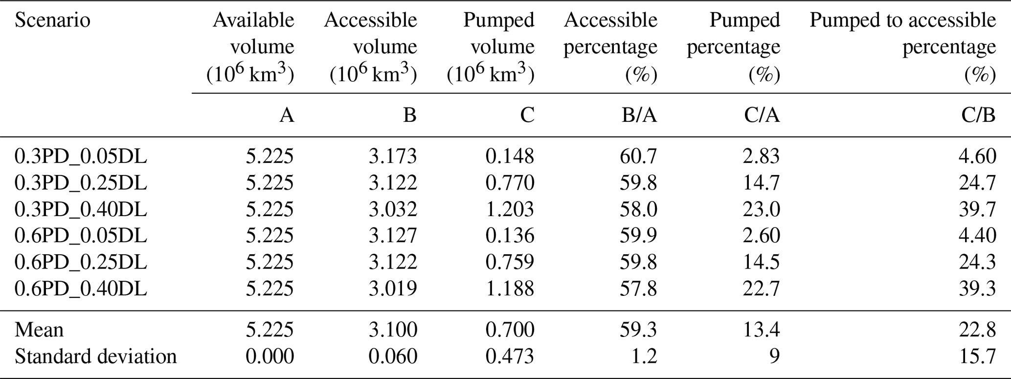
Across the six scenarios modeled in this study, Superwell delineates mean pumped groundwater at 0.7×10⁶ km3 globally (ranging between 0.13 and 1.2×10⁶ km3). This amounts to a quantity of extractable volume that represents only 14 % of globally available groundwater (5.22×10⁶ km3); see Table 1. This represents the upper bound of groundwater volume that could be pumped under constraining factors such as screening criteria, ponded depth target, depletion limit, pumping rate, and aquifer properties among other controls. Extractable volume is driven by constraining factors within each scenario and does not reflect actual demand-driven extraction in aquifers.
Table 1Global available, accessible, and pumped volume in million cubic kilometers along with the percentages of accessible and pumped volumes to available volume and pumped to accessible volume. The ratio of pumped to accessible volume roughly approaches the depletion limit specified in the scenario. PD: ponded depth target in meters; DL: depletion limits as ratios.
Well yield – or pumping rate – reflects grid-specific hydrogeological properties (Eq. 2), impacts extractable groundwater volumes, and determines the energy costs per well and non-energy costs (number of wells) per grid cell which affect unit groundwater cost (Eq. 8). Figure 6a shows optimized well yield averaged over the pumping duration of a cell. Optimization here implies the selection of maximum well yield that location-specific aquifer properties can support. The mapped results are presented as averaged well yield over the pumping duration because pumping rate can be reduced as a result of violating the drawdown criteria (see Sect. 2.2.3 for details). Most regions have well yields less than 2000 m3 d−1 (367 gpm; Fig. 6a). Some cells were skipped due to screening criteria or their inherent aquifer properties that precluded viable pumping rates. These areas predominantly lie in high-altitude mountainous areas, boreal forests, and rainforests, as well as areas with rocky terrains, low saturated thickness, or low permeability.
Figure 6b shows global groundwater pumped volumes under the moderate-depletion (25 %) scenario at the end of the pumping period expressed as ponded depth. Incidentally, many regions currently experiencing water stress around the world coincide with regions showing high groundwater extraction (high availability) within the scenario's constraints (Niazi et al., 2024c). These areas include parts of aquifers in proximity to mountain ranges such as to the east of the Andes, certain pockets in Africa, central and south Asian river basins such as the Indus Basin, and central and western parts of Australia, among others. It is important to note that the extracted volumes of groundwater here only are reflective of the volumes that could be pumped considering aquifer properties, hydrogeological controls, and scenario design and not volume associated with actual historical multisector demand-driven consumption of groundwater.
The evolution of global groundwater pumping over time differs across scenarios mainly driven by defined recharge-adjusted ponded depth targets and depletion limit criteria. Figure 6c and d show how model scenarios influence temporal patterns of global groundwater production. Extractable groundwater becomes exhausted at comparatively steeper rates in initial years under scenarios with lower depletion limits due to some cells reaching exhaustion early in the simulation period. Alternatively, in scenarios with higher ponded depth targets, groundwater is pumped at proportionally higher rates, resulting in higher volumes pumped early on, which, in all cases, results in earlier termination of pumping compared to their lower ponded target counterparts.
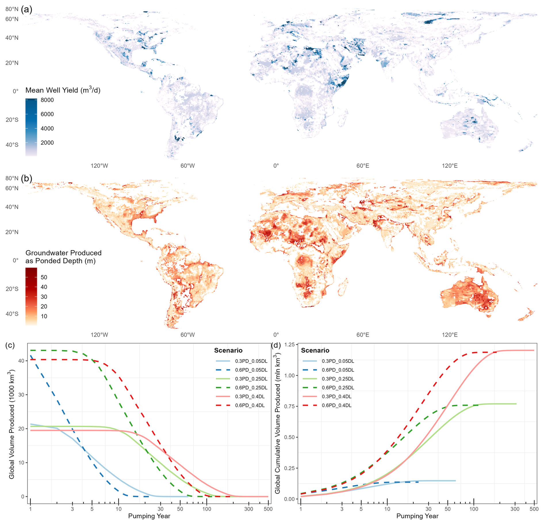
Figure 6Groundwater pumped over model years under scenarios and model constraints: (a) pumping rate (well yield) averaged over the pumping lifetime in a moderate-pumping scenario, (b) volume produced represented as ponded depth (grid cell area normalization) in a moderate-pumping scenario (0.3 m ponded depth and ≤25 % depletion limit), (c) global volume produced over model pumping years, and (d) global cumulative volume produced over model pumping years.
4.2 Cost assessment
A key objective of Superwell is to estimate the cost of groundwater production as a result of groundwater pumping under hydrophysical constraints and scenario specifications over the pumping lifetime of aquifers. This section provides model results about globally gridded energy, non-energy, and unit costs of pumping groundwater.
4.2.1 Energy and non-energy cost of groundwater extraction
Geophysical aspects contributing to energy costs are primarily packaged into the energy required for pumping groundwater from a certain depth at a certain rate over a defined period. Pumping energy required by a given well depends on the initial groundwater depth, the amount of drawdown at the well during pumping, and decline in water depth due to depletion caused by groundwater extraction (Eq. 10). This pumping energy, as shown in Fig. 7 for each grid cell globally in a moderate-depletion scenario, represents a culmination of various dynamics pertaining to well yield and unit lift (Eq. 10) during the pumping phase of Superwell simulations and primarily drives the spatial variability in energy costs in a country.
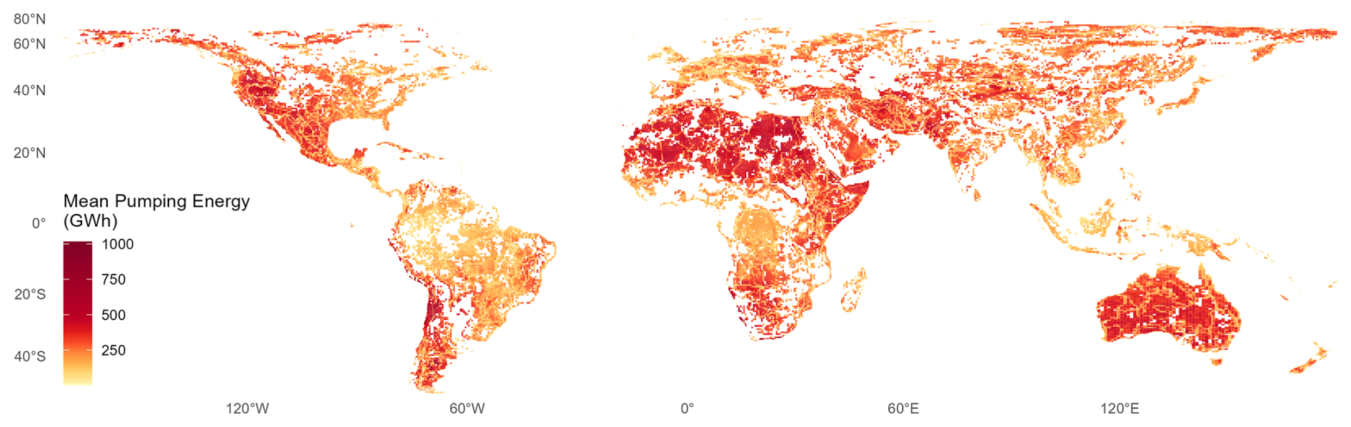
Figure 7Energy required to pump groundwater in a moderate-depletion scenario (GW h; 1 GW h = 3.6 TJ). Pumping energy has been averaged over the entire pumping lifetime for each grid cell.
Energy costs in Fig. 8a account for electricity as the energy source to pump groundwater, introducing an influence of variable electricity rates of each country (Fig. S24) on energy costs of groundwater pumping. Higher mean energy costs are observed in parts of North America, central Asia, and northern and southern extents of Europe, whereas some parts of Africa, South America, and Oceania have lower mean energy costs. As Superwell separately calculates the energy required to pump groundwater (kW h) before applying electricity rates (USD kW h−1) from IEA (2016) to calculate energy costs (USD), see Eq. (9), there is flexibility to estimate costs for alternative energy sources for regions which may have different fuel mixes.
Non-energy costs are influenced by the aquifer class (Fig. S1), well depth (Fig. S19), and parameterization choices for accounting capital and maintenance costs over the well lifetime and loan period. Each of the components of non-energy costs are impacted by exogenous assumptions along with model dynamics. For instance, installation costs are highly influenced by the hydrogeological complexity of the aquifer and the well depth, capital costs are sensitive to the interest rate to account for cost incurred over the lifetime of a well, and maintenance costs are subject to maintenance cost factor (7 % in this version) to account for wear and tear on the pump and need for periodic cleaning or flushing of the well casing. High non-energy costs in regions such as parts of North America, Eurasia, eastern Africa, southwestern India, and southeastern parts of Australia correspond to areas with considerable hydrogeologic complexity and deeper wells incurring high capital and maintenance costs.
The evolution of costs over time, along with the evolution of volume pumped (as shown in Fig. 6), is tracked for each grid cell in each pumping period (yearly in the version of Niazi et al., 2025). Figure 8c shows global annual total costs per well averaged over all grid cells, and Fig. 8d shows total costs for one individual grid cell over model pumping years. The upward trend in capital, maintenance, and energy costs of pumping is attributed to a combination of factors. Specifically, the increasing depth of pumped groundwater, larger drawdown from pumping, increasing well depth, and variable aquifer thicknesses ceasing pumping over time as depletion limits are hit. The rapid decline in global average costs (Fig. 8c) after ≈200 years is due to grid cells going out of production, as can be seen in Fig. 6c (but note that Fig. 8c is normalized by number of wells).
The impact of model features pertaining to changing well characteristics over time (including well deepening, well replacement, and well addition) on the total cost of groundwater extraction is demonstrated using costs of a single grid cell in Fig. 8d. Capital and maintenance costs remain constant until well deepening, well replacement, or well addition happens. Energy costs rise over time as water table depth decreases due to depletion but temporarily drop when/if well deepening occurs, which increases aquifer transmissivity and reduces drawdown for the same pumping rate. Well deepening is used as a first preference when drawdown constraints are violated; the increase in capital and maintenance costs and a decrease in energy costs in year 16 represent the impact of well deepening. The cost of deepening is spread over the well lifetime (20 years in the version of Niazi et al., 2025). The rise in costs in year 20 is due to wells being replaced upon reaching their pre-defined lifetime of 20 years. The period between year 20 and year 36 represents paying off the costs incurred due to both well replacement in year 20 and well deepening in year 16. Pumping rate is reduced as a second preference after violating the drawdown criteria. This occurs in year 48 because the deepening in year 16 extended the well to the full aquifer depth. The reduction in pumping rate results in addition of new wells (with smaller well areas) to compensate for the reduced annual production per well. The addition of wells causes non-energy costs to rise; however, energy costs drop because the reduced pumping rate results in less drawdown and less total lift for the pumps.
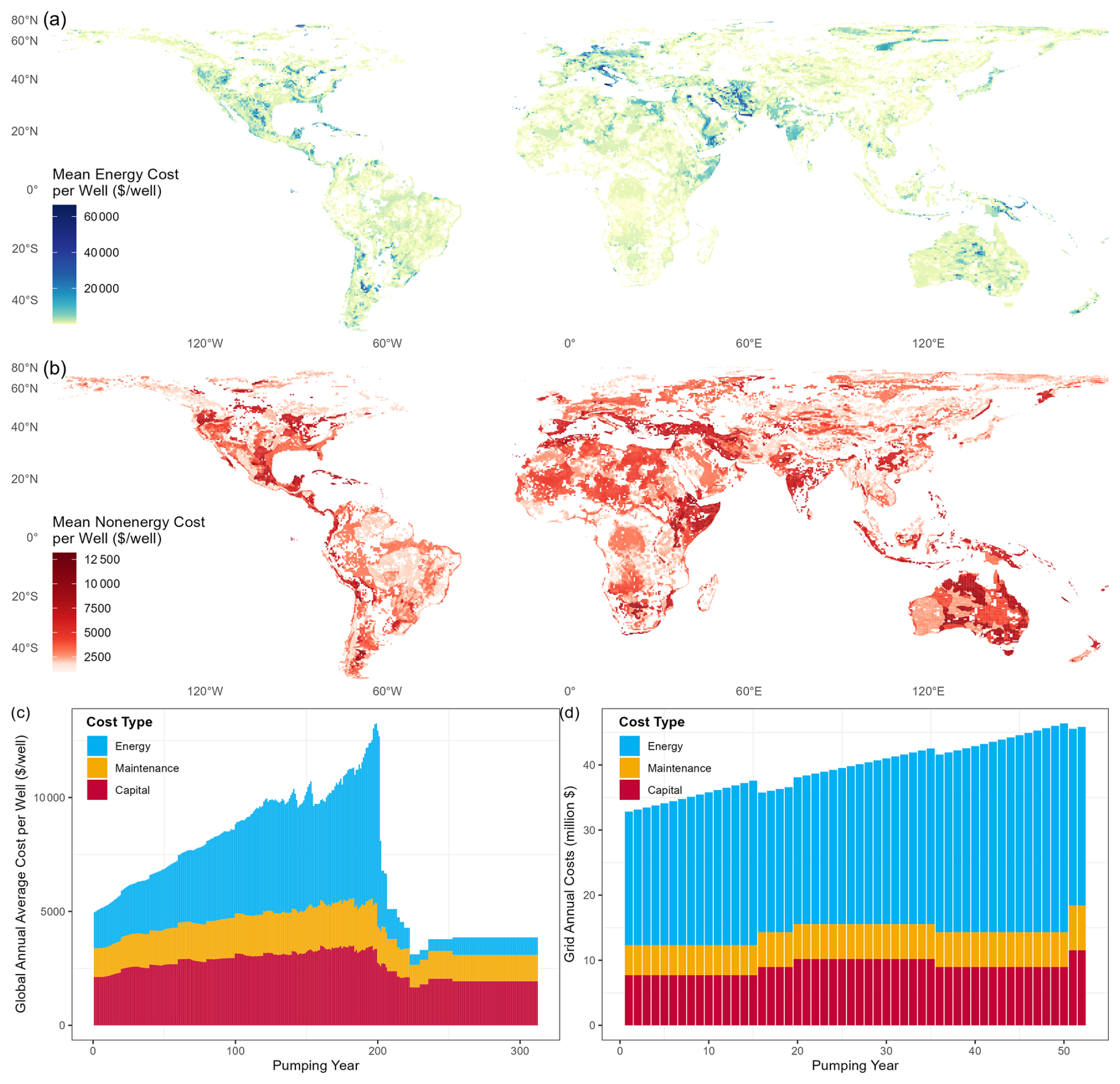
Figure 8Energy and non-energy cost components of the total cost of groundwater extraction in a moderate-depletion scenario: (a) gridded mean global energy cost per well per year averaged over pumping duration; (b) gridded mean global non-energy (capital and maintenance) cost per well per year averaged over pumping duration; (c) global average annual capital, maintenance, and energy cost of groundwater production per well over model pumping years; and (d) grid cell example of annual capital, maintenance, and energy cost of groundwater production over model pumping years.
4.2.2 Unit cost of groundwater extraction
The unit cost of groundwater extraction, calculated as a ratio of the total cost of groundwater extraction and the total volume produced, offers crucial insights into the economic feasibility of groundwater production. Figure 9 shows the mean unit cost over the simulation duration. Hot spots of unit cost are widely distributed over the world, showcasing pronounced heterogeneity due to variability in total groundwater production and drivers of associated costs. Unit cost captures in a single metric the impacts of hydrogeological conditions and model constraints manifested through the production efficiency of aquifers along with physical and economic considerations of infrastructure required for pumping.
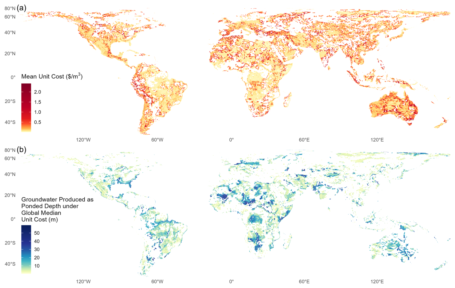
Figure 9(a) Gridded global unit cost map averaged over model years in a moderate-depletion scenario showing a relation between total volume produced and total cost. (b) Total volume produced as ponded depth under the global median unit cost of USD 0.134 m−3.
One of the key advantages of Superwell is to be able to define groundwater extractability at specific cost thresholds for each grid cell (Fig. 9b). In this example, the global median unit groundwater cost (USD 0.123 m−3) is used as the threshold to determine the pumped groundwater volume below the cost threshold at each grid cell. We find that groundwater produced under a global median unit cost of USD 0.123 m−3 amounts to 0.436×10⁶ km3, representing only 8.3 % of the total available groundwater and 56.6 % of the total volume produced in a moderate-depletion scenario. As demonstrated by the patterns in Fig. 9b, Superwell can indicate regions where groundwater is more economical to extract or where it may be more expensive due to various factors, including but not limited to water depth, recharge, hydrogeological parameters, and energy cost of groundwater production. This illustrates the importance of local hydrogeology, pumping scenario, and energy cost in influencing the hydro-economic viability of groundwater production.
4.3 Cost curves of the groundwater supply
Literature values estimate the global average cost of groundwater to be USD 0.02–0.20 m−3 (Llamas et al., 2009). Our results agree with that estimate and are also consistent with more site-specific literature values (Table A2), showing the majority of produced water falling within the USD 0.02–0.20 m−3 range with the most frequent unit cost bin being USD 0.05–0.06 m−3 (Fig. 10). Results of the moderate-depletion case (25 %) are taken as a benchmark with the low-depletion (5 %) and high-depletion (40 %) cases used to provide insight into the sensitivity of groundwater unit costs to these operational decisions. The low-depletion scenario produces the least cumulative volume of groundwater (Fig. 10a), while primarily remaining on the lower unit cost side in the global unit cost distribution (Fig. 10b). The high-depletion scenario extracts most of its cumulative volume at low unit costs (Fig. 10b). It also dominates the higher unit costs of the global distribution, representing continued pumping even in areas where groundwater extraction might not be economically feasible or favorable.
Figure 10b demonstrates, across all depletion criteria cases, that the majority (90 %) of the accessible water was extractable under a unit cost of USD 0.57 m−3, followed by a sharp reduction in the extractable amount at unit costs above USD 0.57 m−3. This behavior can also be observed in inflection points of cost curves given in Fig. 10a for global cost curves and in Fig. 10c for continental-scale cost curves. These inflection points exist at cost levels after which further incremental groundwater extraction would lead to diminishing returns and may prove groundwater production to be economically unfavorable. Globally, there is a peak in the binned unit costs between USD 0.05–0.06 m−3 for the moderate scenario, but lower depletion limits shift the peak towards lower unit costs.
Breaking out cost curves on a continental basis demonstrates large variability in the cost and volume of producible groundwater by continent. Africa and Asia exhibit comparable volumes of cumulative groundwater pumped; however, a skewed peak towards less costly groundwater in Africa suggests a greater availability of cost-effective groundwater compared to Asia. This indicates notable differences in unit cost distributions for different regions even if total groundwater pumped is similar. While increasing costs are expected of any cost curve describing a depletable natural resource, it is worth reiterating that these results reflect the technical challenges (e.g., deeper wells) associated with producing water from greater depths and less favorable hydrogeological settings. The continental (and global) cost curves under the three depletion limits highlight the nonlinear relationship between cumulative volume produced and unit cost.
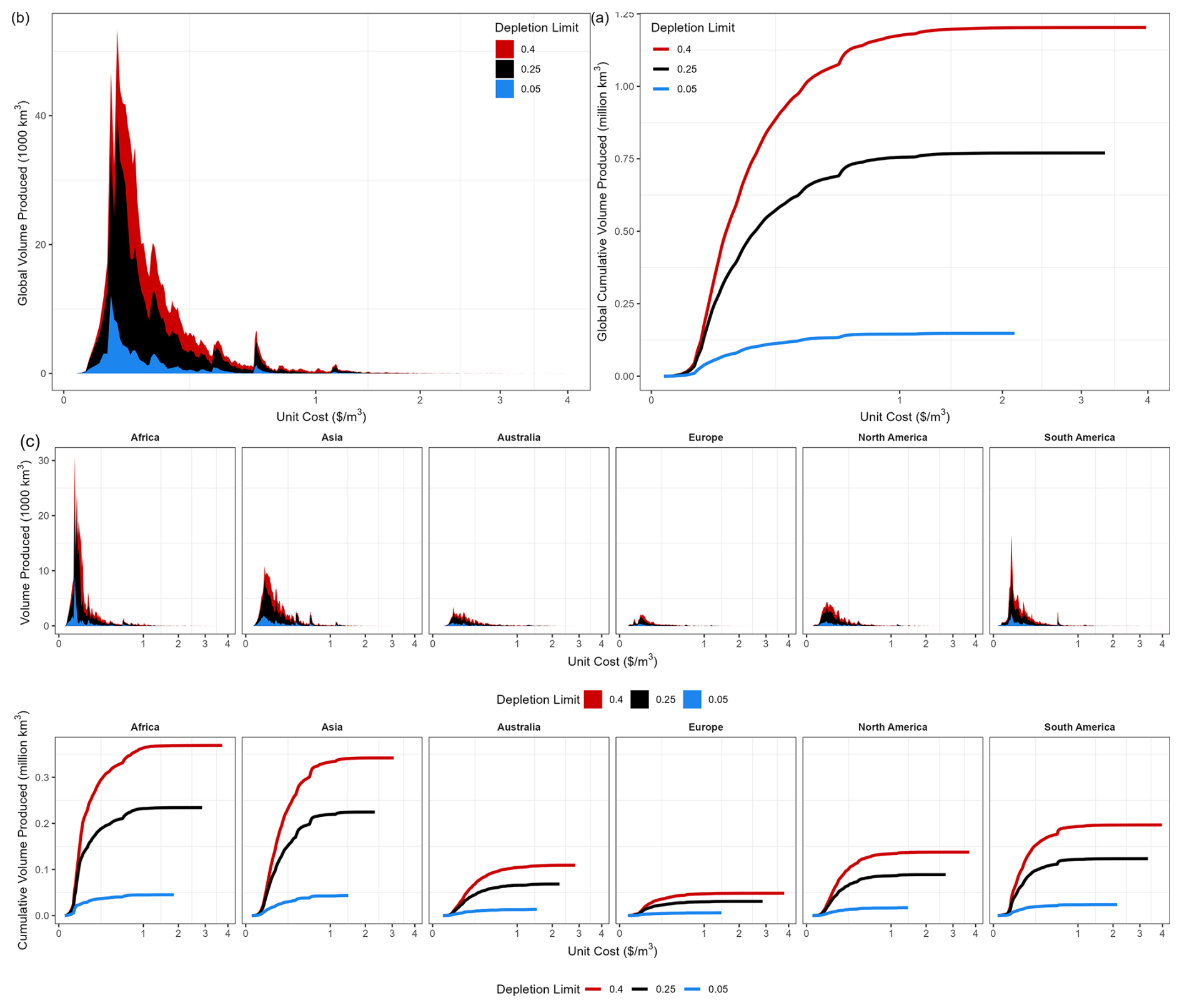
Figure 10Cost curves of the groundwater supply: (a) global cost curve relating cumulative volume and unit cost of pumping, (b) global volume produced per unit cost bin, and (c) cost curves for continents showcasing Superwell's capabilities to produce spatially flexible cost curves.
5.1 Application at flexible scales
With the flexibility of Superwell, cost curves like those shown in Fig. 10 for the world and continents could be generated for each grid cell globally. The finest resolution of the model version presented in this paper (Niazi et al., 2025) is determined by the resolution of input data, whereas the coarser resolutions could be curated using scale mapping files provided with the model. By default, the model provides grid to basin, country, and continent mapping which could be leveraged for spatial aggregation depending on the use case. This adaptability allows Superwell to inform multiple spatially distinct groundwater management strategies by providing scale-specific cost and supply information. Figure 11 demonstrates the applicability of Superwell at spatially flexible scales by breaking out cost curves at various spatial scales.
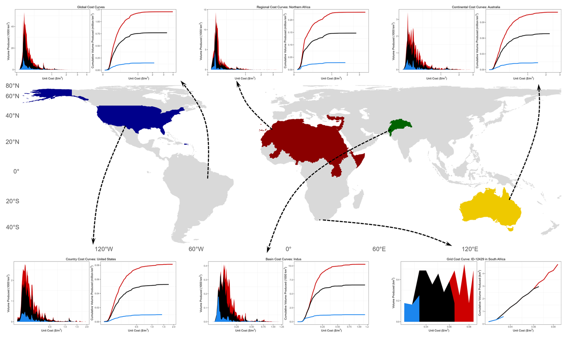
Figure 11Flexible scale application of Superwell to produce groundwater cost curves at various scales ranging from wells to global scales.
Similarly, the model is also flexible in temporal resolution and aggregation, enabling the production of cost curves from years to as long as centuries. The model's temporal resolution is determined by the user; for example, the core version of the model runs on yearly temporal resolution over timescales permitted under model constraints and pumping scenario assumptions. While the underlying methodology is flexible to temporal resolution and assumes annual pumping until depletion limits for practical implementation, the cost curves that are ultimately generated do not have an explicit time component due to temporal aggregation over the pumping lifetime.
5.2 Application for broader multisectoral scopes
We now describe potential integrations of Superwell with various models, illustrating its potential utility for modeling complex human–groundwater interactions. Groundwater cost curves from Superwell can enable modeling the interaction of groundwater cost and supply with water demand, providing insight into multisectoral feedbacks that arise from evolving groundwater costs. The ability to model multisector feedbacks related to groundwater extraction can render valuable insights into the interaction and evolution of complex human and Earth systems under future scenarios.
5.2.1 Multisectoral energy–water–land interactions
Complex human and Earth system interactions could be modeled in a class of models identified as integrated human–Earth system models, such as GCAM (Calvin et al., 2019). Water supply in GCAM is determined from competing cost curves between renewable surface water (Kim et al., 2016; Zhao et al., 2024), groundwater resources (Niazi et al., 2024c; Turner et al., 2019a, b; Hejazi et al., 2023), and desalinated water. Each water basin in GCAM undergoes a water price interaction between nonrenewable groundwater (supplied by Superwell derived cost curves), renewable water, and desalinated water to incrementally withdraw water starting from the cheapest source of water. Each unit of water that is further withdrawn causes price increases to account for the potential costs of river rerouting, dam construction, or transportation of renewable water and the increased costs for extracting deep nonrenewable groundwater. As the price of water extraction increases, a resultant increase in price across end-use sectors occurs, decreasing the profitability of agricultural commodities and increasing the cost of non-agricultural water-demanding sectors (such as municipal water) which may cause production shifts to more economically and environmentally favorable conditions (Kyle et al., 2023; Calvin et al., 2019; Zhang et al., 2024). Such interactions are possible in other modeling frameworks as well with appropriate integration of cost curves derived from Superwell.
5.2.2 Human feedback
In an initial pilot application, Superwell was integrated with a national-scale farm agent-based model of irrigation cropping decisions in the continental United States (CONUS; Yoon et al., 2024). In the agent-based model, ≈50 000 farm agents are deployed across the continental United States at ° resolution (following the North American Land Data Assimilation System grid), with the farms considering irrigation water allocation decisions under changing hydrologic conditions. The farms are treated as profit-maximizing firms, determining cropped areas based on crop prices, production costs (including the costs of producing water for irrigation), crop irrigation needs, and irrigation water availability. The farm agents adopt a positive mathematical programming approach (Howitt, 1995), calibrated to historical data of cropped areas, water availability conditions, and economic conditions. In the pilot application, the farm agent-based model is integrated with two hydrologic sub-models that capture surface water and groundwater availability and cost, with Superwell providing the latter capability.
To align with the spatial delineation of farm agents, Superwell is implemented at ° resolution over the continental United States, with each grid cell assumed to represent an independent groundwater system. The coupled farm ABM–groundwater model abstracts an agricultural groundwater wellfield onto each grid cell, with individual wells uniformly dispersed over the grid cell following Superwell's methodology around designing well spacings that will accommodate sufficient pumping for agricultural needs. For each grid cell, Superwell is run prior to model integration, generating ≈50 000 pre-processed groundwater cost curves.
The cost curves from Superwell in turn serve as a simple lookup table for each farm to track the evolution of groundwater costs and availability over time. In a coupled simulation, the model keeps track of cumulative groundwater production for each grid cell, with the associated point on the groundwater cost curves providing farm agents with the availability and cost of groundwater at that particular state. These inputs from the groundwater cost curves serve as inputs to the farm's cropping decision problem, with the unit cost of groundwater input as a production cost variable and the groundwater production capacity as a resource constraint in the agent's profit-maximization formulation. The Superwell approach serves as a compact and efficient simulator of groundwater cost and response for effective incorporation into the CONUS-scale agent-based model that allows for dynamic agent response to changing groundwater conditions, adding only trivial computational cost and software complexity to the integrated model design.
6.1 Historically calibrated groundwater depletion
In its current implementation, groundwater extraction in Superwell is estimated over model pumping years which do not represent actual yearly extraction or depletion trends. As such, calibrating against historical depletion in each grid cell to provide historically relevant cost estimates and initialize future projections using realistic extraction trends would be an area of improvement for initial model years. As a first step, one could find local regions with sufficient data availability (historical groundwater production and annual estimates of groundwater cost) to evaluate how well the default Superwell parameters reproduce groundwater cost evolution. Local calibration could involve adjusting assumed aquifer properties (porosity and K) and costs (energy, installation costs) to better re-create historical cost and depletion trends. However, this would be limited in many regions by a lack of data (gridded groundwater costs, depletion trends, etc.) at a global scale. As an intermediate step, future work should consider constraining depletion trends on a larger spatial scale to match larger-scale observed depletion trends, thus more accurately capturing spatial variability of groundwater extraction and its associated extraction costs.
6.2 Demand-driven extraction constraints
Superwell currently optimizes pumping rates to choose the maximum allowable rate that a grid cell can support under hydrogeological controls and scenario constraints. Ideally, the pumping rate would be driven by sectoral groundwater demands in a grid cell to ensure realistic estimates of infrastructure requirements for pumping – for example, coupling Superwell with models projecting water demands, such as Tethys (Khan et al., 2023), to inform cost curves that are generated and dynamically updated based on end-use requirements of groundwater. However, the competition between surface water and groundwater must be dynamically represented to support projections into the future (a recent example of modeling structure being GCAM–GLORY, Zhao et al., 2024). This would allow constraining the model using demand-driven pumping rates that are more realistic and enable exploration of pumping and cost dynamics under more realistic societal consumption scenarios.
6.3 Surface and groundwater feedbacks
Groundwater pumping interacts with numerous surface and subsurface hydrological processes such as streamflow, evaporation, discharge, capture, lateral flow, and recharge. These surface–groundwater interactions can impact groundwater fluxes, net groundwater depletion, and associated extraction costs. Recharge, lateral flows (de Graaf and Stahl, 2022), and capture could contribute to a slower decline in water depth in some places which can impact energy and unit costs of groundwater production. Superwell could be coupled to lightweight hydrological emulators (e.g., Xanthos; Liu et al., 2018) or hydrological models (e.g., mosartwmpy; Thurber et al., 2021; Abeshu et al., 2023) to further enhance representation of surface–groundwater interactions while simulating pumping and associated costs in a fast and flexible way. Incorporating these processes within Superwell would improve estimated production costs for both renewable and nonrenewable groundwater.
6.4 Spatial screening
Groundwater extraction is not only deemed feasible on a physical hydrogeological basis but by other factors, such as land use and spatial planning of regions. Currently Superwell screens out grid cells with inland lakes and cells which exhibit conditions that are hydrogeologically unfavorable or do not support viable pumping rates or model constraints. This process screens out about 48 % of grid cells which are physically infeasible in the current version (Niazi et al., 2025). However, these criteria could be extended to other topographical controls such as by factoring in infrastructure development planning or restricting pumping based on the ecological sensitivity of the area.
6.5 Improved, disaggregated, and downscaled datasets
Superwell is designed to operate on spatially and temporally flexible scales, making the resolution and quality of input data a determinant of model resolution. Better and finer-scale estimates of model inputs such as aquifer thickness, depth to water, porosity, permeability, hydrogeological categorization, country-specific interest rates, and long-term inflation estimates would improve the quality of estimates of groundwater availability, extractable volumes, and cost estimates. Similarly, global data on observed well counts and well properties, including diameter, depth, capacity, and installation cost rates, would help improve assumptions about well attributes, making estimates of installation and capital costs more realistic and spatially relevant, and in some cases help validate model outputs, too.
Another opportunity to improve the model's cost accounting of non-energy costs is by collecting and applying country-specific interest rates to amortize the installation and capital costs of wells. This would be supplemented by using country-specific installation cost rates (cost per unit depth of well) to better reflect spatially relevant labor and machinery costs while calculating well installation costs. Lastly, energy supplied for pumping groundwater could be expanded to diesel, solar, and other primary energy sources given their wide use for groundwater pumping in various parts of the world (Balasubramanya et al., 2024). This would not only upgrade Superwell's ability to better represent the fuel mix of energy use for groundwater pumping but would also improve both energy and non-energy cost estimates since each country would have regionally heterogeneous energy cost rates for different fuels and different capital costs for various energy transformation technologies.
Superwell presents a computationally robust integrated hydro-economic framework that incorporates physical groundwater pumping dynamics, recharge, and economic formulations to offer a more comprehensive and internally consistent analysis of global groundwater cost and supply. Unit costs of groundwater production are estimated by modeling the pumping volumes and associated total costs required for groundwater production. Unit cost captures in a single metric the impacts of hydrogeological conditions and model constraints manifested through the production efficiency of aquifers along with physical and economic considerations of infrastructure required for pumping. Superwell determines pumping volumes in a physically realistic way by taking into account aquifer properties (e.g., recharge rates and hydrogeological controls on pumping rates) and modeling well hydraulics. Pumping volumes along with dynamic updating of well attributes over time are used to track annual accounting of capital, maintenance, and energy costs of groundwater production over the pumping lifetime of wells.
Offering a lightweight, fast, and flexible model design that is adaptable across both spatial and temporal scales, Superwell facilitates exploration of user-defined scenarios of groundwater production by varying aquifer depletion limits, annual pumping targets, and annual (days/year) and total pumping duration (number of years), among other exploratory dimensions. This enables the investigation of infrastructure requirements (e.g., number of wells and area served) and associated installation and operational costs to meet pumping targets under the influence of scenario-specific settings and grid-level hydrogeological controls. Superwell's flexible and robust design also offers promising feasibility for dynamic coupling with other models, such as integrated human–Earth system, global hydrological, hydro-economic, agent-based, or multisector dynamics models. Outputs of Superwell, such as unit costs or cost curves, could also be used directly in conjunction with other classes of models to help expand our understanding of groundwater accessibility; cost of supply; and its multi-scale, multisector interactions across the globe.
An application of Superwell on a 0.5° scale globally using geo-processed hydrogeological datasets and six scenarios designed by combining depletion limits and ponded depth targets shows that groundwater production and associated cost dynamics exhibit considerable complexity due to the spatial heterogeneity in hydrogeological conditions and nonlinear processes determining pumping rates and cost accounting over the pumping lifetime of wells. Using global geo-processed datasets of hydrological properties on a 0.5° scale, we find 5.22×10⁶ km3 of groundwater is available in storage globally, with 60 % being physically accessible as a result of screening aquifer properties unfavorable for pumping and only 14 % being extractable for human use over the pumping lifetime across the six scenarios explored in this study. Cost assessment using global groundwater supply–cost curves suggests that most nonrenewable groundwater in storage is extractable at costs lower than USD 0.57 m−3 globally, while half of the volume remains extractable under USD 0.108 m−3.
In summary, Superwell's methodology to produce cost curves accounts for well hydraulics, hydrogeological controls, and pumping scenario constraints on a globally gridded and yearly resolution, with all elements pertaining to resolution, aquifer depletion targets, or decisions regarding pumping regimes implemented in a flexible model design. Its spatially and temporally flexible structure, currently demonstrated on a yearly 0.5° scale globally, allows the production of unit cost from well-to-global spatial scales over yearly-to-centennial temporal horizons. Superwell advances the range of tools and capabilities available to produce cost curves of the groundwater supply at diverse spatiotemporal resolutions. These curves can be used to conduct integrated hydro-economic analyses of water resources or multisector dynamics at the intersection of energy, water, and land systems.
Algorithm A1 describes the overall logic used in Superwell to simulate groundwater extraction dynamics and costs to eventually calculate long-term cost curves of groundwater extraction (Niazi et al., 2025).
Algorithm A1Superwell (https://github.com/JGCRI/superwell, last access: 17 February 2025).
inputs.csv.params.csv.inputs.csv, scenario assumptions params.csv, and other input filesTheis solution and initialize Dataframe that tracks annual pumping and cost metrics.Theis and determine the largest Q that meets the maximum drawdown criteriaviable Qviable QDataframe; and update variable arrays for next annual pumping iterationTable A1Global groundwater volume estimates (million cubic kilometers) as reported by previous studies.
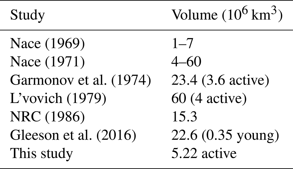
Table A2Previously reported groundwater unit costs. Note that these costs are representative of groundwater production from active water supply aquifers and do not necessarily represent the average unit costs of groundwater across all existing aquifers or of nonrenewable groundwater sources as considered by this study.
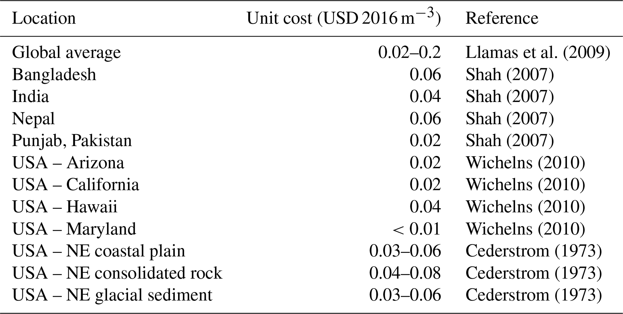
The open-source code repository of Superwell is available at https://github.com/JGCRI/superwell (last access: 17 February 2025). The minted version for version 1.1 is available at https://doi.org/10.5281/zenodo.14583794 (Niazi et al., 2025). The markdown (*.md) files in https://github.com/JGCRI/superwell provide detailed documentation on usage and description of contents of files and scripts.
Model data for both geo-processed inputs (Niazi et al., 2024b) and simulated model outputs (Niazi et al., 2024a) are hosted and minted on MSD-LIVE. Input data located at https://doi.org/10.57931/2484226 contain geo-processed global hydrogeologic datasets of aquifer properties on a 0.5° scale (Niazi et al., 2024b). Outputs located at https://doi.org/10.57931/2307832 include globally gridded groundwater extraction volumes and costs produced from Superwell simulations under six depletion and ponded depth targets (Niazi et al., 2024a).
The supplement related to this article is available online at https://doi.org/10.5194/gmd-18-1737-2025-supplement.
All authors have contributed to this work. Conceptualization: MH. Model development: DW, SF, and HN. Analysis: HN and SF. Writing: all authors.
At least one of the (co-)authors is a member of the editorial board of Geoscientific Model Development. The peer-review process was guided by an independent editor, and the authors also have no other competing interests to declare.
The views and opinions expressed in this paper are those of the authors alone.
Publisher's note: Copernicus Publications remains neutral with regard to jurisdictional claims made in the text, published maps, institutional affiliations, or any other geographical representation in this paper. While Copernicus Publications makes every effort to include appropriate place names, the final responsibility lies with the authors.
The authors would like to thank Catherine Yonkofski for her extensive work in the genesis of Superwell and the supporting framework. We would also like to thank Ning Sun for her extensive internal review and valuable feedback during the preparation of this manuscript.
This research was supported by the U.S. Department of Energy (DOE), Office of Science, as part of research in MultiSector Dynamics, Earth and Environmental System Modeling Program. The Pacific Northwest National Laboratory is operated for DOE by Battelle Memorial Institute under contract DE-AC05-76RL01830.
This paper was edited by Christian Folberth and reviewed by three anonymous referees.
Abeshu, G. W., Tian, F., Wild, T., Zhao, M., Turner, S., Chowdhury, A. F. M. K., Vernon, C. R., Hu, H., Zhuang, Y., Hejazi, M., and Li, H.-Y.: Enhancing the representation of water management in global hydrological models, Geosci. Model Dev., 16, 5449–5472, https://doi.org/10.5194/gmd-16-5449-2023, 2023. a
Advisor, H.: Average Costs per Foot of Well Drilling & Digging, https://www.homeadvisor.com/cost/landscape/drill-a-well/#costs (last access: August 2018), 2018. a
Alam, M. F.: Evaluating the benefit-cost ratio of groundwater abstraction for additional irrigation water on global scale, Student thesis, http://urn.kb.se/resolve?urn=urn:nbn:se:kth:diva-199089 (last access: 17 February 2025), 2016-12-28T13:41:19.323+01:00, 2016. a
Alam, M. F., McClain, M., Sikka, A., and Pande, S.: Understanding human–water feedbacks of interventions in agricultural systems with agent based models: a review, Environ. Res. Lett., 17, 103003, https://doi.org/10.1088/1748-9326/ac91e1, 2022. a, b
Balasubramanya, S., Garrick, D., Brozović, N., Ringler, C., Zaveri, E., Rodella, A.-S., Buisson, M.-C., Schmitter, P., Durga, N., Kishore, A., Minh, T. T., Kafle, K., Stifel, D., Balasubramanya, S., Chandra, A., and Hope, L.: Risks from solar-powered groundwater irrigation, Science, 383, 256–258, https://doi.org/10.1126/science.adi9497, 2024. a
Bierkens, M., De Graaf, I. E., Lips, S., Perrone, D., Reinhard, A. S., Jasechko, S., van der Himst, T., and van Beek, R.: Global Economic Limits of Groundwater When Used as a Last Resort for Irrigation, Research Square [preprint], https://doi.org/10.21203/rs.3.rs-1874539/v1, 2022. a, b
Bierkens, M. F. P. and Wada, Y.: Non-renewable groundwater use and groundwater depletion: a review, Environ. Res. Lett., 14, 063002, https://doi.org/10.1088/1748-9326/ab1a5f, 2019. a
Brown, R. H., Ferris, J. G., Jacob, C. E., Knowles, D. B., Meyer, R. R., Skibitzke, H. E., and Theis, C. V.: Methods of determining permeability, transmissibility and drawdown, Tech. rep., USGPO, https://pubs.usgs.gov/wsp/1536i/report.pdf (last access: 17 February 2025), 1964. a, b
Burek, P., Satoh, Y., Kahil, T., Tang, T., Greve, P., Smilovic, M., Guillaumot, L., Zhao, F., and Wada, Y.: Development of the Community Water Model (CWatM v1.04) – a high-resolution hydrological model for global and regional assessment of integrated water resources management, Geosci. Model Dev., 13, 3267–3298, https://doi.org/10.5194/gmd-13-3267-2020, 2020. a
Calvin, K., Patel, P., Clarke, L., Asrar, G., Bond-Lamberty, B., Cui, R. Y., Di Vittorio, A., Dorheim, K., Edmonds, J., Hartin, C., Hejazi, M., Horowitz, R., Iyer, G., Kyle, P., Kim, S., Link, R., McJeon, H., Smith, S. J., Snyder, A., Waldhoff, S., and Wise, M.: GCAM v5.1: representing the linkages between energy, water, land, climate, and economic systems, Geosci. Model Dev., 12, 677–698, https://doi.org/10.5194/gmd-12-677-2019, 2019. a, b, c
Canales, M., Castilla-Rho, J., Rojas, R., Vicuña, S., and Ball, J.: Agent-based models of groundwater systems: A review of an emerging approach to simulate the interactions between groundwater and society, Environ. Model. Softw., 175, 105980, https://doi.org/10.1016/j.envsoft.2024.105980, 2024. a
Castilla-Rho, J. C., Rojas, R., Andersen, M. S., Holley, C., and Mariethoz, G.: Social tipping points in global groundwater management, Nat. Hum. Behav., 1, 640–649, https://doi.org/10.1038/s41562-017-0181-7, 2017. a, b, c
Cederstrom, D. J.: Cost analysis of ground-water supplies in the North Atlantic region, 1970, US Government Printing Office, https://pubs.usgs.gov/wsp/2034/report.pdf (last access: 17 February 2025), 1973. a, b, c
Davidsen, C., Liu, S., Mo, X., Rosbjerg, D., and Bauer-Gottwein, P.: The cost of ending groundwater overdraft on the North China Plain, Hydrol. Earth Syst. Sci., 20, 771–785, https://doi.org/10.5194/hess-20-771-2016, 2016. a, b
de Graaf, I. E. M. and Stahl, K.: A model comparison assessing the importance of lateral groundwater flows at the global scale, Environ. Res. Lett., 17, 044020, https://doi.org/10.1088/1748-9326/ac50d2, 2022. a
de Graaf, I. E. M., Sutanudjaja, E. H., van Beek, L. P. H., and Bierkens, M. F. P.: A high-resolution global-scale groundwater model, Hydrol. Earth Syst. Sci., 19, 823–837, https://doi.org/10.5194/hess-19-823-2015, 2015. a, b, c
de Graaf, I. E. M., van Beek, R. L. P. H., Gleeson, T., Moosdorf, N., Schmitz, O., Sutanudjaja, E. H., and Bierkens, M. F. P.: A global-scale two-layer transient groundwater model: Development and application to groundwater depletion, Adv. Water Resour., 102, 53–67, https://doi.org/10.1016/j.advwatres.2017.01.011, 2017. a
Dolan, F., Lamontagne, J., Link, R., Hejazi, M., Reed, P., and Edmonds, J.: Evaluating the economic impact of water scarcity in a changing world, Nat. Commun., 12, 1915, https://doi.org/10.1038/s41467-021-22194-0, 2021. a
Döll, P. and Fiedler, K.: Global-scale modeling of groundwater recharge, Hydrol. Earth Syst. Sci., 12, 863–885, https://doi.org/10.5194/hess-12-863-2008, 2008. a, b, c
Fan, Y., Li, H., and Miguez-Macho, G.: Global Patterns of Groundwater Table Depth, Science, 339, 940–943, https://doi.org/10.1126/science.1229881, https://doi.org/10.1126/science.1229881, 2013. a, b
Fenichel, E. P., Abbott, J. K., Bayham, J., Boone, W., Haacker, E. M. K., and Pfeiffer, L.: Measuring the value of groundwater and other forms of natural capital, P. Natl. Acad. Sci. USA, 113, 2382–2387, https://doi.org/10.1073/pnas.1513779113, 2016. a
Fisher-Vanden, K. and Weyant, J.: The Evolution of Integrated Assessment: Developing the Next Generation of Use-Inspired Integrated Assessment Tools, Annu. Rev. Resour. Econ., 12, 471–487, https://doi.org/10.1146/annurev-resource-110119-030314, 2020. a
Foster, T., Brozović, N., and Butler, A. P.: Analysis of the impacts of well yield and groundwater depth on irrigated agriculture, J. Hydrol., 523, 86–96, https://doi.org/10.1016/j.jhydrol.2015.01.032, 2015. a
Foster, T., Brozović, N., and Speir, C.: The buffer value of groundwater when well yield is limited, J. Hydrol., 547, 638–649, https://doi.org/10.1016/j.jhydrol.2017.02.034, 2017. a
Garmonov, I., Konoplyantsev, A., and Lushnikova, N.: The World Water Balance and Water Resources of the Earth, Hydrometeoizdat, 48–50, 1974. a, b, c
Gleeson, T., Wada, Y., Bierkens, M. F. P., and van Beek, L. P. H.: Water balance of global aquifers revealed by groundwater footprint, Nature, 488, 197–200, https://doi.org/10.1038/nature11295, 2012. a
Gleeson, T., Moosdorf, N., Hartmann, J., and van Beek, L. P. H.: A glimpse beneath earth's surface: GLobal HYdrogeology MaPS (GLHYMPS) of permeability and porosity, Geophys. Res. Lett., 41, 3891–3898, https://doi.org/10.1002/2014GL059856, 2014. a, b
Gleeson, T., Befus, K. M., Jasechko, S., Luijendijk, E., and Cardenas, M. B.: The global volume and distribution of modern groundwater, Nat. Geosci., 9, 161–167, https://doi.org/10.1038/ngeo2590, 2016. a, b, c, d, e, f
Gleeson, T., Wagener, T., Döll, P., Zipper, S. C., West, C., Wada, Y., Taylor, R., Scanlon, B., Rosolem, R., Rahman, S., Oshinlaja, N., Maxwell, R., Lo, M.-H., Kim, H., Hill, M., Hartmann, A., Fogg, G., Famiglietti, J. S., Ducharne, A., de Graaf, I., Cuthbert, M., Condon, L., Bresciani, E., and Bierkens, M. F. P.: GMD perspective: The quest to improve the evaluation of groundwater representation in continental- to global-scale models, Geosci. Model Dev., 14, 7545–7571, https://doi.org/10.5194/gmd-14-7545-2021, 2021. a, b
Glotfelty, M. F. (Ed.): The art of water wells: technical and economic considerations for water well siting, design, and installation, NGWA Press, National Ground Water Association, ISBN 1-56034-048-7, 2019. a
Gorelick, S. M. and Zheng, C.: Global change and the groundwater management challenge, Water Resour. Res., 51, 3031–3051, https://doi.org/10.1002/2014WR016825, 2015. a
Grogan, D. S., Wisser, D., Prusevich, A., Lammers, R. B., and Frolking, S.: The use and re-use of unsustainable groundwater for irrigation: a global budget, Environ. Res. Lett., 12, 034017, https://doi.org/10.1088/1748-9326/aa5fb2, 2017. a
Hanasaki, N., Kanae, S., Oki, T., Masuda, K., Motoya, K., Shirakawa, N., Shen, Y., and Tanaka, K.: An integrated model for the assessment of global water resources – Part 1: Model description and input meteorological forcing, Hydrol. Earth Syst. Sci., 12, 1007–1025, https://doi.org/10.5194/hess-12-1007-2008, 2008. a
Harou, J. J., Pulido-Velazquez, M., Rosenberg, D. E., Medellín-Azuara, J., Lund, J. R., and Howitt, R. E.: Hydro-economic models: Concepts, design, applications, and future prospects, J. Hydrol., 375, 627–643, https://doi.org/10.1016/j.jhydrol.2009.06.037, 2009. a, b
Hejazi, M., Santos Da Silva, S. R., Miralles-Wilhelm, F., Kim, S., Kyle, P., Liu, Y., Vernon, C., Delgado, A., Edmonds, J., and Clarke, L.: Impacts of water scarcity on agricultural production and electricity generation in the Middle East and North Africa, Front. Environ. Sci., 11, 1082930, https://doi.org/10.3389/fenvs.2023.1082930, 2023. a, b, c
Howitt, R. E.: Positive mathematical programming, Am. J. Agric. Econ., 77, 329–342, https://doi.org/10.2307/1243543, 1995. a
IEA, I. E. A.: Energy Prices and Taxes, 2016, https://doi.org/10.1787/energy_tax-v2016-3-en, 2016. a, b
Jacob, C. E.: Drawdown Test to Determine Effective Radius of Artesian Well, T. Am. Soc. Civ. Eng., 112, 1047–1064, https://doi.org/10.1061/TACEAT.0006033, 1947. a
Jasechko, S. and Perrone, D.: Global groundwater wells at risk of running dry, Science, 372, 418–421, https://doi.org/10.1126/science.abc2755, 2021. a
Jasechko, S., Seybold, H., Perrone, D., Fan, Y., Shamsudduha, M., Taylor, R. G., Fallatah, O., and Kirchner, J. W.: Rapid groundwater decline and some cases of recovery in aquifers globally, Nature, 625, 715–721, https://doi.org/10.1038/s41586-023-06879-8, 2024. a
Kahil, T., Albiac, J., Fischer, G., Strokal, M., Tramberend, S., Greve, P., Tang, T., Burek, P., Burtscher, R., and Wada, Y.: A nexus modeling framework for assessing water scarcity solutions, Curr. Opin. Env. Sust., 40, 72–80, https://doi.org/10.1016/j.cosust.2019.09.009, 2019. a
Kanazawa, M. T.: Econometric estimation of groundwater pumping costs: A simultaneous equations approach, Water Resour. Res., 28, 1507–1516, https://doi.org/10.1029/92WR00198, 1992. a
Katsifarakis, K. L.: Groundwater Pumping Cost Minimization – an Analytical Approach, Water Resour. Manage., 22, 1089–1099, https://doi.org/10.1007/s11269-007-9212-x, 2008. a
Katsifarakis, K. L., Nikoletos, I. A., and Stavridis, C.: Minimization of Transient Groundwater Pumping Cost – Analytical and Practical Solutions, Water Resour. Manage., 32, 1053–1069, https://doi.org/10.1007/s11269-017-1854-8, 2018. a
Keppo, I., Butnar, I., Bauer, N., Caspani, M., Edelenbosch, O., Emmerling, J., Fragkos, P., Guivarch, C., Harmsen, M., Lefèvre, J., Le Gallic, T., Leimbach, M., McDowall, W., Mercure, J. F., Schaeffer, R., Trutnevyte, E., and Wagner, F.: Exploring the possibility space: taking stock of the diverse capabilities and gaps in integrated assessment models, Environ. Res. Lett., 16, 053006, https://doi.org/10.1088/1748-9326/abe5d8, 2021. a, b, c
Khan, Z., Thompson, I., Vernon, C. R., Graham, N. T., Wild, T. B., and Chen, M.: Global monthly sectoral water use for 2010–2100 at 0.5° resolution across alternative futures, Sci. Data, 10, 201, https://doi.org/10.1038/s41597-023-02086-2, 2023. a
Kim, S. H., Hejazi, M., Liu, L., Calvin, K., Clarke, L., Edmonds, J., Kyle, P., Patel, P., Wise, M., and Davies, E.: Balancing global water availability and use at basin scale in an integrated assessment model, Clim. Change, 136, 217–231, https://doi.org/10.1007/s10584-016-1604-6, 2016. a, b
Klassert, C., Yoon, J., Sigel, K., Klauer, B., Talozi, S., Lachaut, T., Selby, P., Knox, S., Avisse, N., Tilmant, A., Harou, J. J., Mustafa, D., Medellín-Azuara, J., Bataineh, B., Zhang, H., Gawel, E., and Gorelick, S. M.: Unexpected growth of an illegal water market, Nat. Sustain., 6, 1406–1417, https://doi.org/10.1038/s41893-023-01177-7, 2023. a, b
Konikow, L. F. and Kendy, E.: Groundwater depletion: A global problem, Hydrogeol. J., 13, 317–320, https://doi.org/10.1007/s10040-004-0411-8, 2005. a
Korus, J. T. and Burbach, M. E.: Analysis of aquifer depletion criteria with implications for groundwater management, Great Plains Res., 19, 187–200, 2009. a, b
Kyle, P., Ollenburger, M., Zhang, X., Niazi, H., Durga, S., and Ou, Y.: Assessing Multi-Dimensional Impacts of Achieving Sustainability Goals by Projecting the Sustainable Agriculture Matrix Into the Future, Earth's Future, 11, e2022EF003323, https://doi.org/10.1029/2022EF003323, 2023. a
Lall, U., Josset, L., and Russo, T.: A Snapshot of the World's Groundwater Challenges, Annu. Rev. Environ. Resour., 45, 171–194, https://doi.org/10.1146/annurev-environ-102017-025800, 2020. a
Liu, Y., Hejazi, M., Li, H., Zhang, X., and Leng, G.: A hydrological emulator for global applications – HE v1.0.0, Geosci. Model Dev., 11, 1077–1092, https://doi.org/10.5194/gmd-11-1077-2018, 2018. a
Llamas, M. R., Martiìnez-Cortina, L., and Mukherji, A. (Eds.): Water Ethics, Marcelino Botín Water Forum 2007, CRC Press, Boca Raton, FL, ISBN 978-0-203-87543-8, 2009. a, b
L'vovich, M. I.: World water resources and their future, American Geophysical Union, ISBN 978-1-118-66483-4, 1979. a, b, c
McGuire, V. L. and Strauch, K. R.: Water-level and recoverable water in storage changes, High Plains Aquifer, predevelopment to 2019 and 2017 to 2019, USGS, https://doi.org/10.3133/sir20235143, 2024. a
McGuire, V. L., Johnson, M., Schieffer, R., Stanton, J., Sebree, S., and Verstraeten, I. M.: Water in storage and approaches to ground-water management, High Plains aquifer, 2000, vol. 1243, US Geological Survey Reston, VA, USA, https://pubs.usgs.gov/circ/2003/circ1243/pdf/C1243_v1.pdf (last access: 17 February 2025), 2003. a
Medellin-Azuara, J., MacEwan, D., Howitt, R. E., Koruakos, G., Dogrul, E. C., Brush, C. F., Kadir, T. N., Harter, T., Melton, F., and Lund, J. R.: Hydro-economic analysis of groundwater pumping for irrigated agriculture in California's Central Valley, USA, Hydrogeol. J., 23, 1205, https://doi.org/10.1007/s10040-015-1283-9, 2015. a
Messager, M. L., Lehner, B., Grill, G., Nedeva, I., and Schmitt, O.: Estimating the volume and age of water stored in global lakes using a geo-statistical approach, Nat. Commun., 7, 13603, https://doi.org/10.1038/ncomms13603, 2016. a, b, c
Mora, M., Vera, J., Rocamora, C., and Abadia, R.: Energy efficiency and maintenance costs of pumping systems for groundwater extraction, Water Resour. Manage., 27, 4395–4408, https://doi.org/10.1080/07900627.2014.935302, 2013. a
Müller Schmied, H., Cáceres, D., Eisner, S., Flörke, M., Herbert, C., Niemann, C., Peiris, T. A., Popat, E., Portmann, F. T., Reinecke, R., Schumacher, M., Shadkam, S., Telteu, C.-E., Trautmann, T., and Döll, P.: The global water resources and use model WaterGAP v2.2d: model description and evaluation, Geosci. Model Dev., 14, 1037–1079, https://doi.org/10.5194/gmd-14-1037-2021, 2021. a, b
Nace, R. L.: Water, earth, and man: a synthesis of hydrology, geomorphology, and socio-economic geography, Routledge, ISBN 1000384810, 1969. a, b, c
Nace, R. L.: Scientific framework of the world water balance, United Nations Educational, Scientific and Cultural Organization, Technical Papers in Hydrology, Volume 7, Document code: SC.70/XXI.7/A, 1971. a, b, c
Narayanamoorthy, A.: Groundwater depletion and water extraction cost: some evidence from South India, Int. J. Water Resour. Dev., 31, 604–617, https://doi.org/10.1080/07900627.2014.935302, 2015. a
Niazi, H., Ferencz, S., Yoon, J., Graham, N., Wild, T., Hejazi, M., Watson, D., and Vernon, C.: Globally Gridded Groundwater Extraction Volumes and Costs under Six Depletion and Ponded Depth Targets, MSD Live [data set], https://doi.org/10.57931/2307832, 2024a. a, b, c, d
Niazi, H., Watson, D., Hejazi, M., Yonkofski, C., Ferencz, S., Vernon, C., Graham, N., Wild, T., and Yoon, J.: Global Geo-processed Data of Aquifer Properties by 0.5° Grid, Country and Water Basins, MSD Live [data set], https://doi.org/10.57931/2484226, 2024b. a, b, c, d
Niazi, H., Wild, T. B., Turner, S. W. D., Graham, N. T., Hejazi, M., Msangi, S., Kim, S., Lamontagne, J. R., and Zhao, M.: Global peak water limit of future groundwater withdrawals, Nat. Sustain., 7, 413–422, https://doi.org/10.1038/s41893-024-01306-w, 2024c. a, b, c, d, e, f
Niazi, H., Vernon, C., nkholod, and nealtg.: JGCRI/superwell: v1.1 (v1.1), Zenodo [code], https://doi.org/10.5281/zenodo.14583794, 2025. a, b, c, d, e, f, g, h
NRC, N. R. C.: Global change in the geosphere‐biosphere: initial priorities for an IGBP, vol. 7, Chap. 6, 72–86, National Academy Press, NASA-CR-176519, 1986. a, b, c
Reinecke, R., Gnann, S., Stein, L., Bierkens, M., de Graaf, I., Gleeson, T., OudeEssink, G., Sutanudjaja, E., Ruz-Vargas, C., Verkaik, J., and Wagener, T.: Considerable gaps in our global knowledge of potential groundwater accessibility, Earth ArXiv, https://doi.org/10.31223/X5SM0R, 2023. a, b, c
Richts, A., Struckmeier, W. F., and Zaepke, M.: WHYMAP and the Groundwater Resources Map of the World 1:25,000,000, pp. 159–173, Springer Netherlands, Dordrecht, ISBN 978-90-481-3426-7, https://doi.org/10.1007/978-90-481-3426-7_10, 2011. a, b, c
Rodríguez-Flores, J. M., Valero Fandiño, J. A., Cole, S. A., Malek, K., Karimi, T., Zeff, H. B., Reed, P. M., Escriva-Bou, A., and Medellín-Azuara, J.: Global Sensitivity Analysis of a Coupled Hydro-Economic Model and Groundwater Restriction Assessment, Water Resour. Manage., 36, 6115–6130, https://doi.org/10.1007/s11269-022-03344-5, 2022. a
Salem, G. S. A., Kazama, S., Shahid, S., and Dey, N. C.: Impacts of climate change on groundwater level and irrigation cost in a groundwater dependent irrigated region, Agric. Water Manage., 208, 33–42, https://doi.org/10.1016/j.agwat.2018.06.011, 2018. a
Scanlon, B. R., Fakhreddine, S., Rateb, A., de Graaf, I., Famiglietti, J., Gleeson, T., Grafton, R. Q., Jobbagy, E., Kebede, S., Kolusu, S. R., Konikow, L. F., Long, D., Mekonnen, M., Schmied, H. M., Mukherjee, A., MacDonald, A., Reedy, R. C., Shamsudduha, M., Simmons, C. T., Sun, A., Taylor, R. G., Villholth, K. G., Vörösmarty, C. J., and Zheng, C.: Global water resources and the role of groundwater in a resilient water future, Nat. Rev. Earth Environ., 4, 87–101, https://doi.org/10.1038/s43017-022-00378-6, 2023. a
Schewe, J., Heinke, J., Gerten, D., Haddeland, I., Arnell Nigel, W., Clark Douglas, B., Dankers, R., Eisner, S., Fekete Balázs, M., Colón-González Felipe, J., Gosling Simon, N., Kim, H., Liu, X., Masaki, Y., Portmann Felix, T., Satoh, Y., Stacke, T., Tang, Q., Wada, Y., Wisser, D., Albrecht, T., Frieler, K., Piontek, F., Warszawski, L., and Kabat, P.: Multimodel assessment of water scarcity under climate change, P. Natl. Acad. Sci. USA, 111, 3245–3250, https://doi.org/10.1073/pnas.1222460110, 2014. a
Shah, T.: The groundwater economy of South Asia: an assessment of size, significance and socio-ecological impacts, 7–36, CABI, Wallingford, UK, 2007. a, b, c, d
Siebert, S., Burke, J., Faures, J. M., Frenken, K., Hoogeveen, J., Döll, P., and Portmann, F. T.: Groundwater use for irrigation – a global inventory, Hydrol. Earth Syst. Sci., 14, 1863–1880, https://doi.org/10.5194/hess-14-1863-2010, 2010. a
Sophocleous, M.: The origin and evolution of safe-yield policies in the Kansas Groundwater Management Districts, Nat. Resour. Res., 9, 99–110, https://doi.org/10.1023/A:1010139325667, 2000. a
Srikrishnan, V., Lafferty, D. C., Wong, T. E., Lamontagne, J. R., Quinn, J. D., Sharma, S., Molla, N. J., Herman, J. D., Sriver, R. L., Morris, J. F., and Lee, B. S.: Uncertainty Analysis in Multi-Sector Systems: Considerations for Risk Analysis, Projection, and Planning for Complex Systems, Earth's Future, 10, e2021EF002644, https://doi.org/10.1029/2021EF002644, 2022. a
Steward, D. R., Bruss, P. J., Yang, X., Staggenborg, S. A., Welch, S. M., and Apley, M. D.: Tapping unsustainable groundwater stores for agricultural production in the High Plains Aquifer of Kansas, projections to 2110, P. Natl. Acad. Sci. USA, 110, E3477–E3486, https://doi.org/10.1073/pnas.1220351110, 2013. a
Strand, J.: The full economic cost of groundwater extraction (English). Policy Research working paper, no. WPS 5494 Washington, DC, World Bank, http://documents.worldbank.org/curated/en/592401468314702740 (last access: 17 February 2025), 2010. a
Sutanudjaja, E. H., van Beek, R., Wanders, N., Wada, Y., Bosmans, J. H. C., Drost, N., van der Ent, R. J., de Graaf, I. E. M., Hoch, J. M., de Jong, K., Karssenberg, D., López López, P., Peßenteiner, S., Schmitz, O., Straatsma, M. W., Vannametee, E., Wisser, D., and Bierkens, M. F. P.: PCR-GLOBWB 2: a 5 arcmin global hydrological and water resources model, Geosci. Model Dev., 11, 2429–2453, https://doi.org/10.5194/gmd-11-2429-2018, 2018. a
Suter, J. F., Rouhi Rad, M., Manning, D. T., Goemans, C., and Sanderson, M. R.: Depletion, climate, and the incremental value of groundwater, Resour. Energ. Econ., 63, 101143, https://doi.org/10.1016/j.reseneeco.2019.101143, 2021. a
Theis, C. V.: The relation between the lowering of the Piezometric surface and the rate and duration of discharge of a well using ground-water storage, Eos, Transactions American Geophysical Union, 16, 519–524, https://doi.org/10.1029/TR016i002p00519, 1935. a, b, c
Thurber, T., Vernon, C. R., Sun, N., Turner, S. W., Yoon, J., and Voisin, N.: mosartwmpy: A Python implementation of the MOSART-WM coupled hydrologic routing and water management model, J. Open Source Softw., 6, 3221, https://doi.org/10.21105/joss.03221, 2021. a
Turner, S. W. D., Hejazi, M., Calvin, K., Kyle, P., and Kim, S.: A pathway of global food supply adaptation in a world with increasingly constrained groundwater, Sci. Total Environ., 673, 165–176, https://doi.org/10.1016/j.scitotenv.2019.04.070, 2019a. a, b
Turner, S. W. D., Hejazi, M., Yonkofski, C., Kim, S. H., and Kyle, P.: Influence of Groundwater Extraction Costs and Resource Depletion Limits on Simulated Global Nonrenewable Water Withdrawals Over the Twenty-First Century, Earth's Future, 7, 123–135, https://doi.org/10.1029/2018EF001105, 2019b. a, b, c, d, e
USDA, U. S. D. O. A.: Irrigation and Water Management, https://www.nass.usda.gov/Surveys/Guide_to_NASS_Surveys/Farm_and_Ranch_Irrigation/index.php (last access: 20 April 2024), 2024. a, b
Verkaik, J., Sutanudjaja, E. H., Oude Essink, G. H. P., Lin, H. X., and Bierkens, M. F. P.: GLOBGM v1.0: a parallel implementation of a 30 arcsec PCR-GLOBWB-MODFLOW global-scale groundwater model, Geosci. Model Dev., 17, 275–300, https://doi.org/10.5194/gmd-17-275-2024, 2024. a
Vinca, A., Parkinson, S., Byers, E., Burek, P., Khan, Z., Krey, V., Diuana, F. A., Wang, Y., Ilyas, A., Köberle, A. C., Staffell, I., Pfenninger, S., Muhammad, A., Rowe, A., Schaeffer, R., Rao, N. D., Wada, Y., Djilali, N., and Riahi, K.: The NExus Solutions Tool (NEST) v1.0: an open platform for optimizing multi-scale energy–water–land system transformations, Geosci. Model Dev., 13, 1095–1121, https://doi.org/10.5194/gmd-13-1095-2020, 2020. a, b
Weyant, J.: Some Contributions of Integrated Assessment Models of Global Climate Change, Rev. Env. Econ. Policy, 11, 115–137, https://doi.org/10.1093/reep/rew018, 2017. a
Wichelns, D.: Agricultural Water Pricing: United States, Tech. rep., 2010. a, b, c, d
Wild, T. B., Niazi, H., Graham, N. T., Birnbaum, A. N., Zhao, M., Lamontagne, J., Kim, S. H., Chowdhury, A., Msangi, S., and Zhang, Y.: Water and Global Change: An Integrated Modeling Perspective, in: AGU Fall Meeting Abstracts, 2023, H24B–1, https://ui.adsabs.harvard.edu/abs/2023AGUFM.H24B...1W/abstract (last access: 17 February 2025), 2023. a
Yoon, J., Klassert, C., Selby, P., Lachaut, T., Knox, S., Avisse, N., Harou, J., Tilmant, A., Klauer, B., Mustafa, D., Sigel, K., Talozi, S., Gawel, E., Medellín-Azuara, J., Bataineh, B., Zhang, H., and Gorelick, S. M.: A coupled human–natural system analysis of freshwater security under climate and population change, P. Natl. Acad. Sci. USA, 118, e2020431118, https://doi.org/10.1073/pnas.2020431118, 2021. a, b
Yoon, J., Romero-Lankao, P., Yang, Y. C. E., Klassert, C., Urban, N., Kaiser, K., Keller, K., Yarlagadda, B., Voisin, N., Reed, P. M., and Moss, R.: A Typology for Characterizing Human Action in MultiSector Dynamics Models, Earth's Future, 10, e2021EF002641, https://doi.org/10.1029/2021EF002641, 2022. a
Yoon, J., Voisin, N., Klassert, C., Thurber, T., and Xu, W.: Representing farmer irrigated crop area adaptation in a large-scale hydrological model, Hydrol. Earth Syst. Sci., 28, 899–916, https://doi.org/10.5194/hess-28-899-2024, 2024. a
Zhang, X., Sabo, R., Rosa, L., Niazi, H., Kyle, P., Byun, J. S., Wang, Y., Yan, X., Gu, B., and Davidson, E. A.: Nitrogen management during decarbonization, Nat. Rev. Earth Environ., 5, 717–731, https://doi.org/10.1038/s43017-024-00586-2, 2024. a
Zhao, M., Wild, T. B., Graham, N. T., Kim, S. H., Binsted, M., Chowdhury, A. F. M. K., Msangi, S., Patel, P. L., Vernon, C. R., Niazi, H., Li, H.-Y., and Abeshu, G. W.: GCAM–GLORY v1.0: representing global reservoir water storage in a multi-sector human–Earth system model, Geosci. Model Dev., 17, 5587–5617, https://doi.org/10.5194/gmd-17-5587-2024, 2024. a, b
- Abstract
- Introduction
- Approach
- Model diagnostics
- Results
- Model application and use cases
- Current limitations and future directions
- Conclusions
- Appendix A: Superwell algorithm
- Code availability
- Data availability
- Author contributions
- Competing interests
- Disclaimer
- Acknowledgements
- Financial support
- Review statement
- References
- Supplement