Quantitative sub-ice and marine tracing of Antarctic sediment provenance (TASP v1.0)

Ice sheet models should be able to accurately simulate palaeo ice sheets to have confidence in their projections of future polar ice sheet mass loss and resulting global sea level rise. This requires accurate reconstructions of the extent and flow patterns of palaeo ice sheets using real-world data. Such reconstructions can be achieved by tracing the detrital components of offshore sedimentary records back to their source areas on land. For Antarctica, however, sediment provenance data and ice sheet model results have not been directly linked, despite the complementary information each can provide on the other. Here, we present a computational framework (Tracing Antarctic Sediment Provenance, TASP) that predicts marine geochemical sediment provenance data using the output of numerical ice sheet modelling. The ice sheet model is used to estimate the spatial pattern of erosion potential and to trace ice flow pathways. Beyond the ice sheet margin, approximations of modern detrital particle transport mechanisms using ocean reanalysis data produce a good agreement between our predictions for the modern ice sheet–ocean system and seabed surface sediments. These results show that the algorithm could be used to predict the provenance signature of past ice sheet configurations. TASP currently predicts neodymium isotope compositions using the PSUICE3D ice sheet model, but thanks to its design it could be adapted to predict other provenance indicators or use the outputs of other ice sheet models.

1 Introduction

1.1 Motivation and aims

Ice flow pathways and ice sheet extent in the geological past have been inferred using sediment provenance studies, which trace marine detrital sediments to their constituent source rocks on the continent (e.g. Cook et al., 2013; Licht and Hemming, 2017; Wilson et al., 2018; Marschalek et al., 2021). However, conclusions about ice sheet extent and flow patterns drawn from such data are typically not constrained by quantitative analysis. This is because, when viewed in isolation, sediment provenance records can only predict where subglacial erosion was taking place but cannot distinguish between changes in ice extent, changes in subglacial conditions that influence erosion rates or changes in glaciomarine sediment transport processes (e.g. Wilson et al., 2018; Golledge et al., 2021). Following Aitken and Urosevic (2021), provenance (P) over time (t) and space (Ω) can be expressed formally as a probability density function, where the product of geological variation in a source region (G_i(Ω)), erosion of that source region (E_i(t,Ω)) and transport potential (T_i(t,Ω)) are summed over all contributing source regions (a, b, … n).

$$\begin{array}{}\text{(1)}& \begin{array}{rl}P\left(t,\mathrm{\Omega }\right)& =G_a\left(\mathrm{\Omega }\right)\cdot E_a\left(t,\mathrm{\Omega }\right)\cdot T_a\left(t,\mathrm{\Omega }\right)+G_{\mathrm{b}}\left(\mathrm{\Omega }\right)\\ & \cdot E_{\mathrm{b}}\left(t,\mathrm{\Omega }\right)\cdot T_{\mathrm{b}}\left(t,\mathrm{\Omega }\right)+\mathrm{\dots }{G}_n\left(\mathrm{\Omega }\right)\\ & \cdot E_n\left(t,\mathrm{\Omega }\right)\cdot T_n\left(t,\mathrm{\Omega }\right)\end{array}\end{array}$$

Although erosion and debris transport processes are often considered when interpreting sediment provenance records, interpretations are typically limited to a “nearest-neighbour” approach, where changes in provenance are attributed to a simple advance or retreat of the ice sheet margin in the vicinity of the core site (e.g. Cook et al., 2013). Unless other processes that influence provenance signatures can be eliminated, these records may be misinterpreted. Numerical modelling offers the potential to make more quantitative estimates of the ice sheet state required to generate observed sediment provenance signatures by predicting the expected provenance of detritus at the ice sheet margin (Aitken and Urosevic, 2021). In this study, we develop an algorithm (Tracing Antarctic Sediment Provenance, TASP; Marschalek, 2023) to predict geochemical sediment provenance data at offshore core sites from the outputs of numerical ice sheet modelling. The overall aim of TASP is therefore to provide more quantitative information on past ice sheet configurations by predicting the provenance signature of these ice sheets.

1.2 The structure of TASP

TASP estimates relative erosion potential and reconstructs the transport pathways of debris from beneath the ice sheet to the seafloor surrounding the continent. This includes representations of the approximate trajectories of debris at the base of the ice sheet, below and in ice shelves, in icebergs and ocean surface currents, in ocean bottom currents, and in gravity flows. Our inclusion of detritus transport in the ocean is a critical component controlling sediment provenance, as most sediment core records are not directly located at the ice sheet margin today and their distance from the ice sheet margin likely varied significantly in the past. Transport of glaciogenic detritus in the ocean must therefore be considered. TASP approximates methods of marine detritus transport by splitting them into three key interacting processes: iceberg rafting and transport in surface currents (Sect. 2.2), bottom current transport (Sect. 2.3), and gravitational downslope processes (Sect. 2.4) (Figs. 1 and 2).

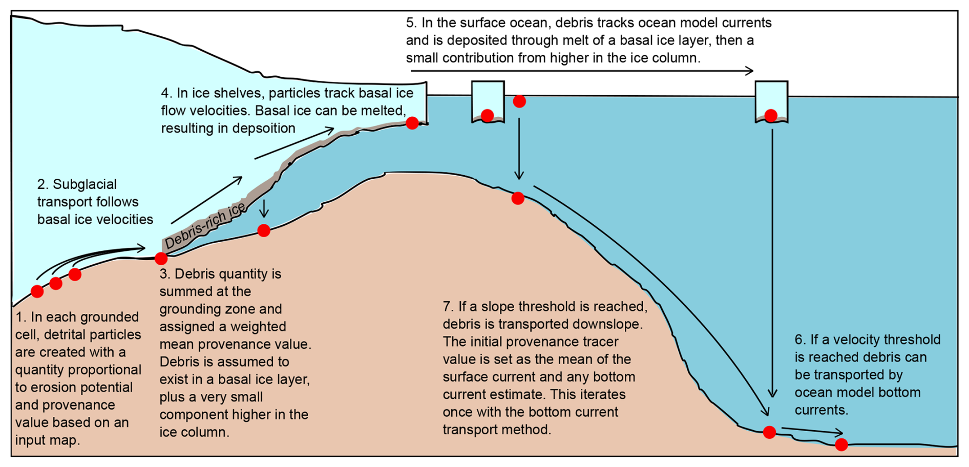
Figure 1 Schematic diagram showing the basic process of debris transport in TASP from source to sink.

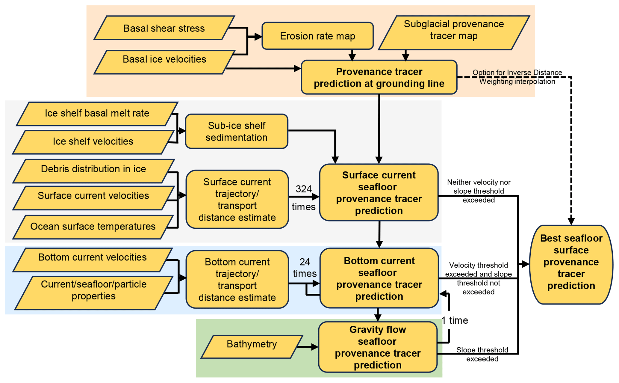
Figure 2 Flowchart outlining the structure of TASP. Coloured boxes indicate the components contained in the “terrestrial.m” (orange), “surf_currents.m” (grey), “bot_currents.m” (blue) and “grav_flows.m” (green) subfunctions.

In summary, TASP is structured in a broadly similar way to how a debris particle might travel from source to sink (Figs. 1 and 2).

1. Debris is generated by glacial erosion, with the relative amount of debris incorporated into basal ice at any location proportional to the product of the basal shear stress and basal ice velocity. Areas with higher basal shear stresses and/or velocities will incorporate more debris. Debris is assigned a provenance tracer value based on a geology-based map of the subglacial source rocks (e.g. Appendix A). Sediment is transported to the grounding zone using basal ice sheet velocities and a flowline algorithm. Because of the time integration of ocean sediment cores (typically 10³–10⁵ years), we ignore deposition and remobilisation along the flowline.

2. As results are compared to marine sediment cores, debris movement from the ice sheet grounding zone to marine sediment core locations must be determined. Assumptions are therefore made regarding the distribution of debris in the ice column and the rate this debris is released from icebergs and ice shelves. These are combined with ice shelf velocities and ocean surface current trajectories to suggest how debris is initially moved from the grounding zone to marine sites.

3. Ocean bottom current velocities are used to determine where these may redistribute debris and the likely trajectories these currents take.

4. If a slope threshold is reached, downslope transport of debris is allowed for. This method is iterated once with the bottom current method, meaning that debris transport can be a combination of all three processes.

5. These different estimates are combined to make a “best estimate” map of seafloor provenance tracer values.

Beyond this overall structure, it is important to understand the following points at the outset.

• TASP does not make any attempt to quantify absolute amounts of debris or sediment. This is because, for provenance purposes, relative amounts of debris are all that is required; for a given offshore sediment sample, the fraction sourced from each rock type in the catchment is what is measured.

• TASP does not step through time simulating debris transport. Samples from sediment cores typically integrate provenance signatures over long timescales, making time-evolving particle tracking at a continental scale unfeasible. Instead, TASP takes a “snapshot” approach throughout, assuming the system is in steady state.

• TASP is written in MATLAB and is external to the ice sheet model code. This approach provides flexibility, with the opportunity to apply it to various existing model experiments. TASP is not model-specific and could be applied to any ice sheet model output, providing key variables (bed elevation, basal shear stress and basal ice velocities with horizontal directional components) are saved.

2 Model description

2.1 Subglacial debris generation and transport

The starting point of the TASP algorithm is an ice sheet model output, which is used to estimate the generation and subglacial transport of debris (Fig. 2). Following the approach of Pollard and DeConto (2019), TASP approximates erosion potential (E) as proportional to the product of basal velocity (u_b) and basal shear stress (τ_b) from the ice sheet model (Table 1):

$$\begin{array}{}\text{(2)}& E={\mathit{\tau }}_{\mathrm{b}}{u}_{\mathrm{b}}k.\end{array}$$

The “quarrying” coefficient k is a parameter dependent on properties including the erodibility of different rock types and other parameters that are unaccounted for. Here, a spatially uniform value of $\mathrm{5.1}\times {\mathrm{10}}^{-\mathrm{10}}$ was used for k, as suggested by Pollard and DeConto (2019). As we are only concerned with relative and not absolute quantities of detritus, the value used will not impact results.

There are continuing difficulties in quantifying processes of erosion and entrainment of subglacial debris, despite extensive study of these topics (Alley et al., 2019). This means that various erosion laws have been employed to recreate glacially eroded landscapes, typically also using an erodibility constant and the ice velocity raised to an exponent, often ∼2 (e.g. Herman et al., 2015). We also note that more sophisticated methods have been previously applied to model erosion beneath alpine glaciers (e.g. Ugelvig et al., 2018; Magrani et al., 2022). Here, we opt to use the erosion law in Eq. (2) as it has been proven to reproduce reasonably accurate modern Antarctic topography starting from a pre-glacial landscape (Pollard and DeConto, 2019) and because using a different erosion law would be unlikely to result in a significantly different pattern of erosion potential, which broadly scales with basal ice velocity and increases towards the ice margin.

We note that where till is present at the ice sheet bed, this will shield the underlying substrate from erosion (Pollard and DeConto, 2003). However, the thickness, distribution and original provenance of a till layer will vary as a function of time and is increasingly uncertain in the past. Accounting for this in TASP would therefore involve incorporating the debris tracing into a time-evolving ice sheet model run, requiring significant extra computational time and negating the strength of TASP as a post-processing tool compatible with any ice sheet model output. Knowing the composition of subglacial sediments to make this useful would also require knowledge of subglacial geology at a far higher resolution than is currently possible. Because of these considerations, in its current form TASP effectively assumes that any till at a given location would be comprised of the bedrock directly beneath it.

Figure 3 Synthetic model test for the terrestrial component. This includes (a) a synthetic provenance tracer input map and (b) an erosion potential map, created using basal shear stress and basal ice velocities that increase away from the centre. Absolute values are not shown as only relative erosion potential is relevant for provenance tracing. Panel (c) shows the radial streamlines in grey and the calculated provenance tracer value at the ice sheet margin.

From the site of debris generation at each grid cell, sediment packages were traced to the grounding line using the MATLAB “streamline” function and the directional components of basal ice velocity (e.g. Fig. 3c). The “streamline” function calculates curves tangential to the velocity vector field (i.e. streamlines) using an Euler integration method from input seed locations. Seed locations were selected based on a user-defined erosion potential threshold, which is set to 0 to include all cells beneath grounded ice. Increasing this threshold would lead to faster run times at the expense of neglecting erosion in areas with low erosion potential. The streamline function is also used in the marine components of TASP (see Sect. 2.2 and 2.3) and is responsible for most of the computational demand.

Using default settings, eight CPUs and 64 GB of memory required a run time of ∼6–8 h on the Imperial College London HPC cluster (AMD EPYC 7742 2.25 GHz processor). Randomly selecting a subset of ocean streamline locations was investigated as a method of reducing this computational cost. However, it was found that any reduction in seed locations notably worsened the match with surface sediment measurements.

Once the streamlines were calculated, provenance tracer values at the grounding zone end locations were set using the provenance tracer values at the streamline start locations defined by a subglacial input map for the given provenance proxy and an erosion potential map. The provenance tracer input map is a critical part of TASP and, given significant uncertainties in the subglacial geology of Antarctica, likely comprises the largest source of error in the results.

Typically, multiple streamlines arrive at a given grounding zone end cell. The final provenance tracer values of grounding zone end cells were therefore calculated as a weighted mean by multiplying the provenance tracer values of each streamline start location by the erosion potential value (E) of the start location, then summing this for all streamlines at a grounding zone end cell. This was then divided by the summed erosion potential of all the streamlines arriving at the grounding zone end cell (i.e. $\sum (E_{i,j}\cdot \mathit{\epsilon }N{d}_{i,j})/\sum E_{i,j}$), where i,j represents all streamline start locations feeding into the grounding zone cell. The provenance tracer values at a given cell in the grounding zone thus reflect integration of the subglacial detritus at all locations upstream weighted to the relative erosion potential. To verify that the terrestrial component of TASP is functioning correctly, an experiment was performed with a square synthetic ice sheet flowing radially outwards. The provenance tracer input was a synthetic grid with values varying between 0 and 9 (Fig. 3a), and erosion potential was set to increase radially from the domain centre (Fig. 3b). As expected, provenance tracer values at the synthetic ice sheet margin reflect the detritus eroded at all areas upstream and was weighted to the erosion potential so that cells near the edge of the domain dominate the provenance signature (Fig. 3c).

Particle transport has been included in many previous studies seeking to examine glacier flow or validate models (e.g. Clarke and Marshall, 2002; Jouvet and Funk, 2014). However, these studies typically focus on tracing ice movement within the ice column for ice core dating (e.g. Clarke and Marshall, 2002) or on alpine glaciers that have a very different spatial scale and topographic or climatological setting to the continental-scale ice sheets that are the focus of TASP (e.g. Jouvet and Funk, 2014). As we are primarily concerned with debris generated at the ice sheet bed, we neglect vertical transport. TASP also assumes all debris generated is advected to the ice sheet margin (i.e. no significant subglacial sedimentation occurs). Furthermore, steady-state ice flow is assumed, allowing any change to ice flow trajectories to be neglected. TASP does not therefore account for transient phenomena such as the centennial stagnation and reactivation of Siple Coast ice streams (Hulbe and Fahnestock, 2007). The time between debris entrainment and deposition offshore may in reality be hundreds to thousands of years, depending on ice velocities. However, the primary goal of TASP is to reproduce long-term, large-scale provenance patterns, such as interglacial ice sheet configurations smaller than that at present; for these, ice flow will be broadly consistent for thousands of years. At the temporal and spatial scales of interest here, the approximations used are considered sufficient to capture the broad-scale trajectories of debris under the ice sheets.

TASP does not account explicitly for detritus transport in subglacial hydrological networks. For ice sheets where there is a general lack of surface melt, such as present-day Antarctica, only basal meltwater feeds subglacial hydrological networks. This steady generation of water results in low water flow speeds and consequently very low sediment fluxes, even during episodic subglacial lake drainage events (Hodson et al., 2016; Alley et al., 2019). Subglacial hydrological networks will, however, evacuate some small amount of sediment beneath such an ice sheet. We suggest this debris transport method can be safely neglected in TASP as the trajectories of this detritus are unlikely to deviate significantly from ice flow vectors at the continental scale of interest here (Willis et al., 2016).

However, in a system with significant surface melt, such as the modern Greenland Ice Sheet or potential palaeo Antarctic ice sheets, subglacial hydrological networks or even proglacial rivers could be more important for transporting detritus. Such debris transport is not yet accounted for in TASP, but subglacial fluvial transport could potentially be incorporated through interfacing with complementary modelling specifically targeting fluvial transport of subglacial sediment (e.g. Delaney et al., 2019; Aitken et al., 2024).

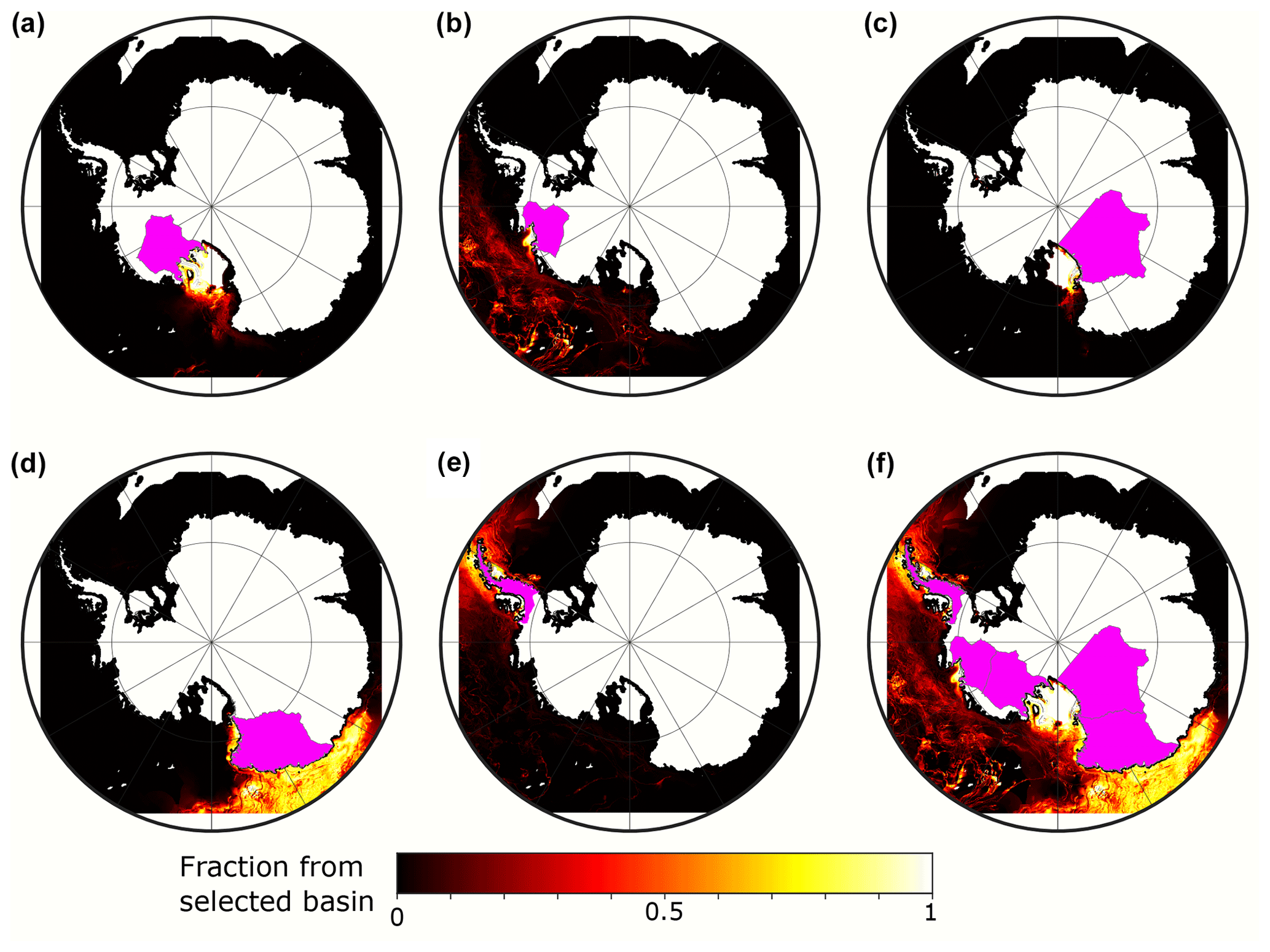
Figure 4 The predicted fraction of offshore sediment originating from five IMBIE drainage basins shown in pink (a–e) and the total fraction from all five selected basins (f).

2.2 Ocean surface currents, iceberg rafting and ice shelves

2.2.1 Debris distribution in the ice column

Before predicting how debris is deposited in the marine realm, it is important to consider the distribution of the debris concentration in the ice column as this is a primary control on marine debris transport. If debris is incorporated further from the edge of an iceberg, more melt needs to occur for it to be released, potentially allowing for a longer transport distance. Observations fully penetrating the ice column are rare, but they show that for continental-scale ice sheets, at least outside of mountainous regions, most glaciogenic debris is concentrated in the basal layers of the ice column, typically the lowermost 2–15 m (Gow et al., 1979; Christoffersen et al., 2010; Shaw et al., 2011; Pettit et al., 2014). Empirical relationships of the distribution of debris within this basal ice layer have been formulated, showing – from the base upwards – a constant debris content for several metres followed by a sharp exponential decay (Yevteyev, 1959), but very few data are available to suggest how typical this relationship is (Drewry and Cooper, 1981). Indeed, it can be assumed to vary significantly between localities depending on factors such as how the debris is incorporated (i.e. shearing and ice deformation vs. basal freeze on; Drewry and Cooper, 1981). Ice sheet basal conditions, including melting and freezing rates and the vertical component of ice flow, thus govern the thickness and nature of this debris-rich basal ice layer (Licht and Hemming, 2017). Conditions at the ice sheet bed are therefore critical (Dowdeswell and Murray, 1990) and result in substantial variations in the distribution of debris in basal ice around Antarctica before the ice reaches the grounding zone.

Above this debris-rich basal ice layer, the debris concentration is strongly influenced by the glaciological setting. For instance, due to a relatively high number of rock outcrops, smaller icebergs calved from glaciers draining through mountainous regions carry more supraglacial debris and englacial debris higher in the ice column than larger tabular icebergs calved from major ice shelves, which may predominantly carry basal debris (e.g. Anderson, 1999). These significant and poorly understood complexities mean estimating a variable debris distribution down the ice column for different regions is beyond the scope of this study. Debris distribution in TASP is simplified by assuming it is the same in all icebergs, although we acknowledge that accounting for a variable debris load would improve the accuracy of the results.

To reflect the potential for limited concentrations of debris higher in the ice column, we include a very low minimum englacial debris content. This is included because for large ice sheets (i) supraglacial debris is very rare but occasionally present (e.g. Evans and Cofaigh, 2003), (ii) englacial debris above basal debris-rich layers has been observed in multiple locations (Nicholls et al., 2012; Winters et al., 2019; Smith et al., 2019) and (iii) iceberg-rafted debris (IBRD) can be transported for hundreds to thousands of kilometres offshore (e.g. Dowdeswell and Murray, 1990; Dowdeswell et al., 1995; Gil et al., 2009). This background debris concentration is set to 10⁻⁵ times the maximum debris load at the base of the ice column based on an assumption of a ∼10 % debris concentration in basal ice vs. ∼0.001 % higher in the ice column (Dowdeswell and Murray, 1990). We find TASP is insensitive to the precise quantity of debris higher the ice column used.

To summarise, TASP assumes debris in the ice column at the grounding zone is distributed predominantly in a debris-rich basal layer, above which there is a very small but finite debris concentration. From an initial debris content at the ice–bed interface (D₀), the debris concentration in the ice (D) at a given height above the ice base (Z) is assumed to decay linearly up the ice column, reaching a minimum “englacial” concentration (D_e):

$$\begin{array}{}\text{(3)}& D=\max \left(D_{\mathrm{e}},D_{\mathrm{0}}\left(\mathrm{1}-{\displaystyle \frac{Z}{Z_{\mathrm{0}}}}\right)\right),\end{array}$$

where Z₀ is the debris-rich basal ice thickness in metres. A value of 4 m was selected for Z₀ based on tuning within the approximate range of observed thicknesses (Sect. 3.2). TASP was found to be relatively insensitive to the value chosen. As summed erosion potentials from the terrestrial component of TASP are saved at the end cells of ice flow trajectories, D₀ is set based on the amount of eroded material reaching these grounding zone cells. Z is a cumulative product of melt rate and the amount of time elapsed, as described in Sect. 2.2.4.

Other options beyond a linear decay in distance from the bed (Eq. 3) were also explored. These included an exponential decline in debris yield:

$$\begin{array}{}\text{(4)}& D=\max \left(D_{\mathrm{e}},D_{\mathrm{0}}\left(-\mathit{\lambda }{\displaystyle \frac{Z}{Z_{\mathrm{0}}}}\right)\right),\end{array}$$

where a decay coefficient λ=5 was selected for rain-out of basal debris over a length of time that agrees closely with more in-depth studies of iceberg rafting (e.g. Hopwood et al., 2019). Experiments were also performed with constant basal debris yield from the basal ice (i.e. D=D₀ while Z<Z₀). However, these changes to debris distribution within the ice had a negligible impact on results.

2.2.2 Representation of ice shelves

Once in contact with the ocean, ice may begin to melt, releasing debris from the ice column. Melting of basal ice may begin before icebergs calve due to the presence of floating ice shelves. Melting at the grounding zone can lead to high accumulation of previously frozen-on basal debris or deforming subglacial till in sedimentary landforms, such as a till delta or grounding-zone wedge (e.g. Alley et al., 1989; Batchelor and Dowdeswell, 2015). Important influences on sub-ice shelf sedimentation include the seaward extent and morphology of the ice shelf, the presence of pinning points that can allow freeze on of new sediment, and the temperature of ocean water reaching the base of the floating ice that governs basal melt and freezing rates (e.g. Smith et al., 2019). These processes often lead to basal detritus being deposited, although debris near the base can also rise in the ice column if net freezing and/or surface ablation occur (Kellogg and Kellogg, 1988; Kellogg et al., 1990; Nicholls et al., 2012).

Beneath ice shelves, debris frozen into the ice will continue to follow ice-flow trajectories and are thus set in TASP by the ice sheet model. Ocean currents beneath ice shelves are very difficult to observe and are thus poorly constrained. TASP therefore assumes that there is no debris transport by ocean currents beneath ice shelves, with debris instead following modelled ice flow trajectories and melting out (or refreezing debris-free ice) at a rate controlled by the estimated sub-ice-shelf melt rate. In the code, ice flow velocities are effectively treated as very slow ocean current velocities, allowing a realistic pattern of melting (thus sedimentation) and freezing beneath ice shelves.

2.2.3 Surface current trajectories

Once calved, iceberg trajectories are a function of surface ocean current velocity, wind velocity and iceberg size; dedicated iceberg models account for such complexities (e.g. Bigg et al., 1997; Hill and Condron, 2014). However, surface current velocities dominate, particularly for large icebergs (Rackow et al., 2017; Wagner et al., 2017). We therefore here use an ocean velocity reanalysis dataset to approximate the pathways that icebergs would be expected to take after calving. This velocity field was used as an input for the MATLAB streamline function, with the end cells of the grounded ice sheet streamlines (i.e. the grounding zone) used as seed locations for the ice shelf–ocean streamlines.

While it is reasonable to assume the velocities of debris beneath an ice shelf are constant through time, using a single snapshot of ocean velocities is not accurate. This is because sea ice variability and weather patterns create substantial seasonal and interannual variations in iceberg pathways estimated from ocean surface current velocities. To account for this effect, debris trajectories are calculated for multiple monthly mean velocities. Debris transport was assumed to follow the trajectories produced by each velocity field.

As we seek to approximate many debris transport mechanisms in a single framework, the method of ocean model particle tracking described here is relatively simple compared to code designed specifically for this task, such as Parcels (Lange and Sebille, 2017) or ROMSPath (Hunter et al., 2022). Such tools are more sophisticated than required for the purposes of TASP, as they for instance operate in 4D and account for particle dispersion. TASP therefore does not seek to replace them; they are instead a potentially useful complement.

2.2.4 Debris distribution along surface current trajectories

Once the trajectories of surface currents have been determined, the debris distribution along each trajectory can be predicted. This is important because where multiple trajectories cross the same ocean cell, there must be a realistic weighting to the different source locations. To achieve this, the subglacial erosion potential values from the terrestrial component feeding into each cell at the grounding zone are summed and used to weight the initial debris concentration in each ocean surface current starting cell.

In the ocean, modern melt rates in TASP are calculated using sea surface temperatures (T_s) corresponding with the monthly ocean surface velocity data used (Zuo et al., 2019; Copernicus Climate Data Store, 2021). Melt rate (M_b) will vary as a function of ocean temperature; we parameterise this from the empirical equation of Russell-Head (1980):

$$\begin{array}{}\text{(5)}& M_{\mathrm{b}}=\mathrm{2.08}\times {\mathrm{10}}^{-\mathrm{7}}(T_{\mathrm{s}}+\mathrm{1.8}{)}^{\mathrm{1.5}},\end{array}$$

where M_b is calculated for every ocean cell for each month in the ocean dataset. Although this does not account for the many complexities associated with calculating iceberg melt that are represented in dedicated iceberg models (e.g. Bigg et al., 1997; Hill and Condron, 2014), it is considered a sufficient simplification for the purposes of TASP.

TASP then loops over each cell in each surface current trajectory, calculating Z_(n) (the thickness of basal ice melted in cell n) as follows:

$$\begin{array}{}\text{(6)}& Z_{\left(n\right)}=Z_{(n-\mathrm{1})}+M_{\mathrm{b}\left(n\right)}\cdot {\displaystyle \frac{\mathrm{\Delta }d}{v_{\mathrm{mag}\left(n\right)}}},\end{array}$$

where Z_(n−1) is the thickness of ice already melted from the “iceberg” in the previous cell, Δd is the distance travelled from the last cell, and v_mag(n) is the magnitude of the velocity in the given cell. The debris yield for the given cell is then given by Eq. (3). In this way, debris from icebergs more proximal to their source location will dominate the provenance signature, but there is the potential for far-travelled icebergs to influence provenance tracer values where more local icebergs are absent.

The relative amount of debris release over time from individual icebergs will, in reality, depend on iceberg size and frequency of overturning, and as such they may be episodic (Drewry and Cooper, 1981; Dowdeswell, 1987; Dowdeswell and Murray, 1990). However, we verify that our equations accurately represent iceberg melt by inputting typical Southern Ocean values for T_s; this produces debris yields over time comparable to those of studies with a more rigorous treatment of iceberg movement and melt (Dowdeswell and Murray, 1990; Hopwood et al., 2019).

To convert this relative debris amount into an estimate of the provenance tracer value for each ocean cell, the provenance tracer value of glaciogenic debris at each ice sheet grounding zone cell was projected along the iceberg paths and weighted based on the debris content of the grounding zone cell and the amount of basal ice melted. Each ocean cell is therefore assigned two values for each streamline: (a) a provenance tracer value and (b) a relative debris amount. For each month in the surface ocean velocity–temperature dataset, a map of provenance tracer values is then calculated based on the debris amount saved for each streamline and the grounding zone provenance tracer value. A mean is then taken of the monthly estimates to produce the final “surface current” provenance value estimate.

Areas with no iceberg tracks over them but within 40 km of an iceberg track were filled using interpolation. This interpolation somewhat accounts for the potential for variations in ocean surface currents that are unresolved here. Furthermore, it is likely that there would be transport of icebergs over more of the seafloor than captured in the years of data feasible to use in TASP over the centuries integrated within most sediment samples of centimetre-scale thickness. A given “iceberg” is therefore not modelled in a true time-evolving manner, as its trajectory is calculated based on a single month's surface current velocity data. Although unrealistic, this simplification was necessary to avoid detailed modelling of icebergs that would need to include additional factors, such as morphology and wind stress (e.g. Rackow et al., 2017).

Sea ice conditions impact iceberg movement and melt, leading to seasonally changing detritus transport in surface currents. We do not explicitly account for sea ice movement but note that the far lower sea surface temperatures in the winter months, when icebergs usually calve less frequently and are frozen into sea ice, will weight our results near the coast towards the summer months.

2.2.5 Suspended sediment

Until now, it has been assumed that debris is transported entirely within ice. This is not realistic, as fine-grained detritus can also derive from meltwater plumes rising from beneath the ice shelf base at the grounding zone (e.g. Lepp et al., 2022). Meltwater plumes can deposit sediment tens of kilometres away from the grounding zone and will track ocean currents (e.g. Smith et al., 2019, and references therein). Furthermore, once melted out of the ice shelf or icebergs, very fine-grained IBRD will not instantaneously fall out of the water column. Instead, silt particles (on the order of 5–50 µm) with slower settling velocities will be transported horizontally as they sink down through the water column over periods of days to months, leading to potential transport distances of tens to thousands of kilometres, depending on grain size and current speed (Azetsu-Scott and Syvitski, 1999).

Meltwater plumes (and fine-grained debris melted out of icebergs) can travel at varying heights in the water column, depending on the relative densities of the plume and surrounding ocean water. Although not explicitly represented in TASP, we argue these debris transport mechanisms will track ocean flow patterns and hence are somewhat represented by the use of both surface and bottom current approximations (see also Sect. 2.3). Given that our provenance tracer value estimate using ocean surface currents represents not only IBRD that immediately settles but also potential settling of fine-grained detritus derived from icebergs and/or meltwater plumes, we refer to the estimate derived from tracking surface currents as the “surface current” method rather than the IBRD method.

2.3 Bottom currents

Iceberg rafting and surface currents are not responsible for all transport of glaciomarine detritus. One key process, especially on the continental rise, is the transport and deposition of predominantly silt- and clay-sized detritus by bottom currents. These currents typically flow parallel to the continental slope where they can influence the movement of detrital particles already in suspension. Bottom currents not only deposit sediments as “contourites” but can also erode and redistribute particles from the seabed surface if their velocities are sufficiently high. Bottom current velocities can occasionally be sufficiently high to remobilise sediment on the continental shelf in addition to in the deep ocean (Ha et al., 2014; Jenkins et al., 2018).

In TASP, bottom currents are defined as the deepest ocean velocity layer. As TASP seeks to represent transport of the <63 µm grain size fraction, it assumes that a current velocity in the range of ∼0.12–0.18 m s⁻¹ is needed to start the resuspension and redistribution of the finest sediment particles (McCave and Hall, 2006; Gross and Williams, 1991). This threshold can vary significantly depending on properties such as the mean grain size, sorting and cohesiveness of the sediment, but tuning this parameter within this range suggested a best match with seafloor surface sediments when a threshold of 0.16 m s⁻¹ is used (Sect. 3.2).

The ocean reanalysis velocity data are unlikely to capture the full variability in bottom current dynamics, which include significant changes in current speed and orientation on timescales as short as hours (e.g. Camerlenghi et al., 1997; Giorgetti et al., 2003). This poses the question as to whether the sedimentary record predominantly reflects an integrated mean of long-term bottom-current flow variability or whether it is dominated by episodes of peak current speed and current direction at these times. Here, it is assumed the latter case applies, and peak flow velocities are assumed to be 2.5 times the monthly mean in the ocean reanalysis product to account for the temporal variability in bottom current strength. This relationship is based on measurements of bottom current strength at mooring sites around a contourite drift on the western Antarctic Peninsula continental rise (Camerlenghi et al., 1997; Giorgetti et al., 2003), which record peak velocities approximately 2 to 3 times greater than mean velocities. The bottom current speed record from the Antarctic Peninsula drift is also comparable with other bottom current records (Gross and Williams, 1991). It is therefore suggested that the aforementioned 0.16 m s⁻¹ threshold speed for the start of resuspension and winnowing is exceeded during times when currents are strongest in areas where mean monthly flow velocity exceeds 0.064 m s⁻¹ in the reanalysis product.

Consequently, all areas where bottom current velocities exceed 0.064 m s⁻¹ are used as source locations for debris. Our approach is supported by the fact that the sortable silt mean size of seafloor surface sediment from another Antarctic Peninsula drift, recovered at a comparable water depth as the mooring measurements, suggests formation under a bottom current with a flow velocity matching the peak speed recorded in the mooring data (Hillenbrand et al., 2021). Detritus entrained in bottom currents is again routed using the MATLAB “streamline” function.

As suspended particles will not be deposited uniformly over a given streamline, deposition over a streamline must be approximated. Although detailed modelling of bottom current erosion, transport, and deposition is beyond the scope of this study, an approximation produces a realistic exponential decay in suspended particle concentration (c) over time (t_s, in seconds):

$$\begin{array}{}\text{(7)}& c=c_{\mathrm{0}}\exp \left(-{\displaystyle \frac{p{t}_{\mathrm{s}}{v}_{\mathrm{s}}}{y}}\right).\end{array}$$

Here, p is the probability of a particle sticking to the ocean floor, v_s is settling velocity and y is the thickness of the layer with suspension load in metres (Einstein and Krone, 1962). As we are not concerned with absolute amounts of sediment, the initial particle concentration (c₀) is irrelevant and set to 1. A value of $\mathrm{3.3}\times {\mathrm{10}}^{-\mathrm{4}}$ m s⁻¹ is used for the settling velocity, which is within the range expected for fine-grained detritus (Einstein and Krone, 1962; McCave, 2005). Suspended particle layer thickness (y) is highly variable and uncertain and was therefore tuned against seafloor surface sediment data, with a value of 15 m selected (Sect. 3.2).

The probability of the particle sticking to the bed (p) in Eq. (7) can be calculated from bottom shear stress, τ_w (N m⁻²), using a critical depositional stress, τ_c (N m⁻²; Einstein and Krone, 1962):

$$\begin{array}{}\text{(8)}& p=\mathrm{1}-{\displaystyle \frac{{\mathit{\tau }}_{\mathrm{w}}}{{\mathit{\tau }}_{\mathrm{c}}}},\end{array}$$

where τ_c is set to 0.08 N m⁻², in line with observed estimates for different classes of sediment that vary between 0.05 and 0.1 N m⁻² (Shi et al., 2015; Lumborg, 2005; McCave, 2008). In turn, τ_w can be approximated as a product of vertically averaged velocity ($\overline{U}$) and water density (ρ) using a quadratic law (Mofjeld, 1988; Garcia and Parker, 1993).

$$\begin{array}{}\text{(9)}& {\mathit{\tau }}_{\mathrm{w}}=\mathit{\rho }{C}_{\mathrm{d}}{\overline{U}}^{\mathrm{2}}\end{array}$$

At the deep-sea water depths of interest here, the drag coefficient, C_d, can be estimated using

$$\begin{array}{}\text{(10)}& C_{\mathrm{d}}={\mathit{\kappa }}^{\mathrm{2}}/{\left[\log \left({\displaystyle \frac{H}{z_{\mathrm{0}}}}\right)-\mathrm{1}\right]}^{\mathrm{2}},\end{array}$$

where H is water depth and z₀ is the roughness length. Here we use $\mathrm{5}\times {\mathrm{10}}^{-\mathrm{4}}$ m for the roughness length, which is a reasonable approximation given that the drag coefficient is insensitive to relatively small changes in water depth in the deep sea (i.e. H≫z₀) (Mofjeld, 1988). Here, κ is the von Kármán constant (0.41). This approximation yields a spatially variable drag coefficient on the order of $\sim {\mathrm{10}}^{-\mathrm{3}}$, which is a magnitude consistent with observations (Umlauf and Arneborg, 2009). For simplicity, the bottom current velocity is assumed to be approximately equal to the depth-averaged velocity.

To set the initial provenance tracer value of detritus mobilised by bottom currents, we use the output from the surface current method. To account for any seasonal changes in bottom current velocity, we then iterate the current tracing (24 months suggested) using the output from the previous month to set the provenance tracer value of sediment eroded where possible. Similar to the surface current estimate, the results for detritus moved by bottom currents are interpolated for 40 km around trajectories to account for unresolved pathways and for the fact that there is relatively little data to constrain modelled bottom current velocities in the ocean reanalysis product.

This approach to bottom current transport assumes the transport along a given monthly mean trajectory occurs under steady-state conditions and does not account for changing currents during the duration of a detrital particle being suspended. This approach is by necessity a major simplification of the treatment of particle transport and sediment remobilisation by bottom currents. Nevertheless, the areas subject to sediment remobilisation are captured alongside the provenance of detritus reaching a given location through bottom current transport.

2.4 Gravitational downslope transport

Substantial volumes of glaciomarine detritus can be moved through gravity-driven downslope processes, such as turbidity currents, slumps and debris flows. To represent these transport mechanisms, the mean provenance tracer values from the surface and bottom current methods at all locations with a slope of >1°, mostly confined to the continental slope, are selected. This slope threshold was selected by tuning within a range of feasible values (Stow, 1994; Sect. 3.2). These grid cells are used as start locations from which the direction of gravitational transport is calculated using the D8 algorithm (O'Callaghan and Mark, 1984), which iterates until a cell is repeated (i.e. an upwards slope is reached). TASP makes no attempt to account for variations in debris load over travel distance along a gravitational transport pathway. This is deemed reasonable, as such paths are unlikely to cross as the direction of travel and will usually be approximately perpendicular to the coast (on the shelf) or the shelf break (on the continental slope) unlike ocean currents. Thus, calculation of the relative quantity of sediment is unnecessary.

Unresolved bathymetric features mean gravitational flows are likely to carry detritus beyond the constraints of the approximate gravity flow paths. The gravitational transport provenance estimate is therefore interpolated. Gravity flows do not necessarily shed their load once the slope falls below a threshold. Turbidity currents, for example, can carry particles over 1000 km (e.g. Mulder, 2011). As our gravity flow paths were already typically 300–600 km long, we interpolate a further 300 km at all locations beyond the shelf break.

Theoretically, the relief on the continental shelf can be sufficient in places for gravity flows to redistribute sediment (e.g. Anderson et al., 1983; Hillenbrand et al., 2005). However, these processes are unlikely to transport significant amounts of sediment at the spatial scales (tens to hundreds of kilometres) considered here, and recent gravitational downslope deposits have only been identified in Antarctica locally on the very rugged, over-deepened inner continental shelf (e.g. Smith et al., 2009; Hogan et al., 2020). Thus, we do not interpolate the gravitational transport provenance estimate on the continental shelf, defined as water depths <1200 m. Although this depth threshold is significantly deeper than the true average water depth of the continental shelf, which varies predominantly between ∼400 and 500 m in Antarctica, using 1200 m avoids inclusion of most over-deepened areas on the innermost shelf close to the present ice sheet margin, where interpolation should be avoided.

Turbidity currents flowing perpendicular to the shelf break down the continental slope can carry suspended particles to locations on the continental rise where they are captured by bottom currents flowing parallel to the margin, i.e. approximately parallel to the shelf break (e.g. Rodrigues et al., 2022b; Hillenbrand et al., 2021). To account for this interaction between gravitational downslope processes and bottom current transport, the output of the gravity flow method was iterated once with the bottom current method described above. Although this approach does not explicitly represent suspended material supplied by gravitational processes that is subsequently captured by bottom currents, using an iterative method does account for particle transport both parallel and perpendicular to the continental margin in both the bottom current and gravitational provenance tracer value estimates.

To ensure that TASP transports particles to sensible areas offshore, we use an idealised provenance tracer map for the IMBIE Antarctic drainage basins (Zwally et al., 2012). Each basin was set to a provenance tracer value of 1 and elsewhere set to 0, and this is repeated for five major drainage sectors in Antarctica: (a) the Siple Coast; (b) the Amundsen Sea; (c) the central Transantarctic Mountains; (d) Victoria Land, Oates Land, and George V Land; and (e) the Antarctic Peninsula. This produced maps of the fraction of sediment derived from each basin (Fig. 4). This demonstrates that TASP captures a pattern of sediment dispersal offshore where sedimentation is concentrated close to the grounding zone and broadly diminishes with distance from the source (e.g. Smith et al., 2019).

2.5 Relative contribution of transport mechanisms

To produce a best estimate seafloor provenance map, it is necessary to apportion the relative contribution of the three marine transport mechanisms (Sect. 2.2–2.4) around the Antarctic continental margin. The TASP best estimate map uses the value for gravity flows where they are present, bottom currents where gravity flows are absent, and surface currents where there is neither a gravity flow nor a bottom current estimate (Fig. 2). Assigning one method to each grid cell is not physically accurate, as all marine transport mechanisms may interact at a given location. However, TASP accounts for this as it uses the surface current estimate as the source of the bottom current estimate and the bottom current and surface current estimate maps as the source for the gravity flow estimate. A major strength of this approach is that it does not require an estimate of the absolute quantity of detritus transported by each mechanism, which is useful given that the rates of these processes are very poorly constrained.

In some settings, marine transport processes can be estimated given observations of geomorphological features (e.g. contourite drifts, channels eroded by turbidity currents), grain size parameters (e.g. content of coarse-grained clasts indicative of IBRD supply, percentage and mean of sortable silt as a proxy for bottom current vigour) and sedimentary structures (e.g. normally graded turbidites, winnowed layers of residual coarse-grained sediments). However, making these inferences requires good coverage with high-resolution bathymetric and seismic data and the collection of numerous sediment cores from targeted locations. Even then, however, it often remains difficult to determine the fraction of the sediment transported by different mechanisms (e.g. Rodrigues et al., 2022a, b). The approach used by TASP is therefore considered a necessary and appropriate simplification.

3 Results when applied to present-day Antarctica

3.1 Selected provenance tracer, study site and input data

An ability to accurately represent the modern system is a pre-requisite for reconstructing sediment provenance in the past. We here apply TASP to the modern Antarctic ice sheets (i.e. East Antarctic Ice Sheet, West Antarctic Ice Sheet (WAIS) and Antarctic Peninsula Ice Sheet). For this case study, the performance of TASP can easily be evaluated because the spatial distribution of provenance proxy measurements in marine sediments is far more complete in recent (i.e. late Holocene to modern) surface sediments than in older, more difficult to date, sediments (e.g. Simões Pereira et al., 2018). This is accompanied by the ability to directly measure ice surface velocities and ice thicknesses. Ice flow drainage pathways and erosion potentials are therefore far more precisely constrained than is possible for past ice sheets. Modern oceanographic data mean marine processes transporting glaciogenic detritus can also be more accurately simulated at the present day. By predicting the provenance signature of the modern Antarctic ice sheets and comparing this to measured seafloor surface sediments, we demonstrate the accuracy of TASP and show that applying it to past ice sheets should produce useful results. Palaeo ice sheet simulations can be input into the current version of TASP. Selecting the “palaeo” option will reduce outputs by not comparing results of the provenance tracing to seafloor surface sediment measurements.

To trace debris transport, a sediment provenance proxy is required. TASP could be adapted for any sediment provenance tracer, such as clay minerals (e.g. Ehrmann et al., 2011), heavy minerals (e.g. Hauptvogel and Passchier, 2012), elemental concentrations (e.g. Monien et al., 2012), clast petrography data (e.g. Sandroni and Talarico, 2011) or detrital mineral ages (e.g. Licht et al., 2014). Each provenance proxy would require a map of its subglacial distribution. In the case of the categorical data (e.g. clast types) or binned distributional data (e.g. specific detrital mineral age populations), TASP would require adapting to account for multiple input maps and saving of multiple output maps with the associated extra memory demand.

However, for this case study TASP targets detrital neodymium (Nd) isotopes, which are expressed simply as a single number, for which TASP is currently designed. Nd isotope compositions are a powerful sediment provenance proxy as all rock-forming minerals incorporate Nd and Sm into their structure, meaning all rock types will be accounted for and are integrated in the provenance signal. Furthermore, Nd isotope compositions are generally unaffected by grain size sorting (Garçon et al., 2013). These factors mean Nd isotope compositions have seen widespread application in Antarctic sediments (e.g. Farmer et al., 2006; van de Flierdt et al., 2007; Roy et al., 2007; Pierce et al., 2017; Simões Pereira et al., 2018). For instance, the proxy has provided evidence for East Antarctic Ice Sheet retreat in the Pliocene and Pleistocene (Cook et al., 2013; Wilson et al., 2018) and marine-based WAIS growth in the Early Miocene (Marschalek et al., 2021).

The ${}^{\mathrm{143}}\mathrm{Nd}{/}^{\mathrm{144}}\mathrm{Nd}$ ratio is typically reported in epsilon notation (ε_Nd), i.e. in parts per 10 000 compared to the modern Chondritic Uniform Reservoir (CHUR; Jacobson and Wasserburg, 1980):

$$\begin{array}{}\text{(11)}& {\mathit{\epsilon }}_{\mathrm{Nd}}=\left({\displaystyle \frac{{\left({}^{\mathrm{143}}\mathrm{Nd}{/}^{\mathrm{144}}\mathrm{Nd}\right)}_{\mathrm{sample}}}{{\left({}^{\mathrm{143}}\mathrm{Nd}{/}^{\mathrm{144}}\mathrm{Nd}\right)}_{\mathrm{CHUR}}}}-\mathrm{1}\right)\times {\mathrm{10}}^{\mathrm{4}}.\end{array}$$

Analytical errors for ε_Nd values are typically ∼0.2 to 0.3 epsilon units (e.g. Farmer et al., 2006; Marschalek et al., 2021).

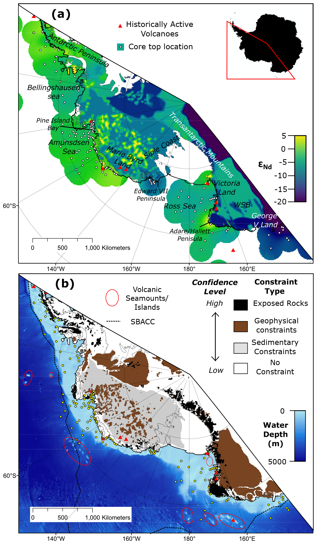
Figure 5 (a) Map of inland ε_Nd values used as an input for the provenance tracing (Appendix A) and interpolated ε_Nd values within 200 km of a marine surface sediment sample with a measured ε_Nd value. Seafloor surface sample locations are shown as white circles, and volcanoes with reported subaerial eruptions in the historic record are shown as red triangles (Patrick and Smellie, 2013). The MEaSUREs grounding line and modern ice (shelf) fronts are indicated using solid grey and black lines, respectively (Rignot et al., 2013; Mouginot et al., 2017). (b) The confidence level of ε_Nd value estimate, displayed on BedMachine bathymetry (Morlighem et al., 2020). Uncertainty levels are classified as exposed rock with ε_Nd data (black); areas with subglacial geology constrained by gravimetric, magnetic, geomorphological, etc., data (brown); areas with few direct constraints, limited to isolated subglacial samples obtained by drilling through the ice (grey); or areas without any rock type constraints, filled using Kriging (white). Volcanic seamounts and islands (e.g. Lawver et al., 2012; Kipf et al., 2014) are circled in red. These features are displayed because they potentially supply additional radiogenic detritus to marine sediments that is unaccounted for in our algorithm. The southern boundary of the Antarctic Circumpolar Current (SBACC) is shown as a dashed black line (Orsi et al., 1995).

Geographically, we examine the region offshore of West Antarctica and adjacent areas of East Antarctica (from approximately 60° W to 140° E; Fig. 5). This spans the location of many existing detrital Nd isotope provenance studies (e.g. Cook et al., 2013; Marschalek et al., 2021) and compilations of the ε_Nd values of continental rocks (e.g. Simões Pereira et al., 2018; Marschalek et al., 2021). Although TASP estimates provenance all around Antarctica, useful results are limited to this extent of compiled literature ε_Nd values. Expanding the useful area of the domain would require additional compilation of bedrock literature data and assumptions regarding subglacial geology (Appendix A). Application of TASP to other ice sheets, such as the Greenland Ice Sheet, is possible but would require some modifications to the model code to account for the different geographic setting. As TASP focuses on marine transport processes and does not represent fluvial sediment transport, it is most applicable to ice sheets with predominantly marine-terminating glaciers.

To assign eroded detritus an ε_Nd value for comparison with offshore records, the first requirement is a spatially continuous estimate of ε_Nd for the study area below grounded ice (Fig. 5a). Constructing this map required the compilation of literature ε_Nd data for different rock types (see Appendix A for a detailed description). This process was aided by an existing compilation of ε_Nd data from the Pacific sector of West Antarctica (Simões Pereira et al., 2018, 2020), extended to the Ross Sea sector (Marschalek et al., 2021). Using a different provenance proxy would require construction of another map for the given provenance tracer.

To assess the accuracy of our sediment provenance tracing algorithm, results were compared to ε_Nd values measured in recent seabed surface sediments (Fig. 5a). These data were compiled from all known literature sources in our study domain (Walter et al., 2000; Roy et al., 2007; van de Flierdt et al., 2007; Pierce et al., 2011; Cook et al., 2013; Struve et al., 2017; Simões Pereira et al., 2018, 2020; Carlson et al., 2021; Shao et al., 2022). New seafloor surface sediment ε_Nd data from the Ross Sea were also included to improve spatial coverage in this area (Table A2).

Table 1 Parameters used in TASP.

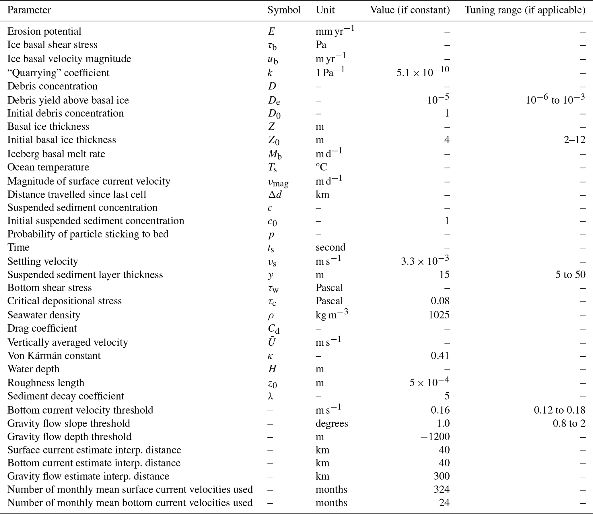
Figure 6 (a) Erosion potential map used to seed start locations. Absolute erosion potential is not given as this is uncertain and not required to predict offshore provenance. (b) Grounded ice streamlines (grey), with points at the end of each streamline coloured according to the ε_Nd value at the streamline start point. A dashed box indicates the location of the inset, which shows more detailed flowlines in the Amundsen Sea Embayment. The colour bar in the centre shows both the erosion potential in panel (a) and the ε_Nd values in panel (b).

To simulate the generation and transport of debris subglacially (Fig. 6), we use a simulation of the modern ice sheet from the model PSUICE3D, which is a finite-difference numerical model with hybrid ice flow dynamics (Pollard and DeConto, 2012). The simulation used (DeConto et al., 2021) closely matches modern observations. It was run at 10 km resolution, although TASP automatically adjusts to match coarser resolutions. Ice shelf melt rates are set by observation over the 2010–2018 period (Adusumilli et al., 2020).

The ORAS5 ocean velocity reanalysis dataset was used to provide temperatures and ocean currents for 324 months spanning January 1993 to December 2019 (27 years; Zuo et al., 2019; Copernicus Climate Data Store, 2021). Experiments with fewer months of data showed that at least 20 years of data are required, with 27 years accurately capturing most annual and interannual variation in iceberg trajectories around Antarctica. However, the ORAS5 ocean velocity reanalysis dataset only extends to 80° S, which does not reach the calving front along parts the Ross and Filchner–Ronne ice shelves. This produced a gap in the velocity field. Simply interpolating available surface ocean velocities did not produce plausible flow directions near the ice sheet margin in the regions not covered by the reanalysis product. Consequently, the mean of the interpolated ocean velocity data and extrapolated ice velocities beyond the ice sheet margin was used after scaling the latter to the mean of local ocean velocities so that they are a consistent order of magnitude.

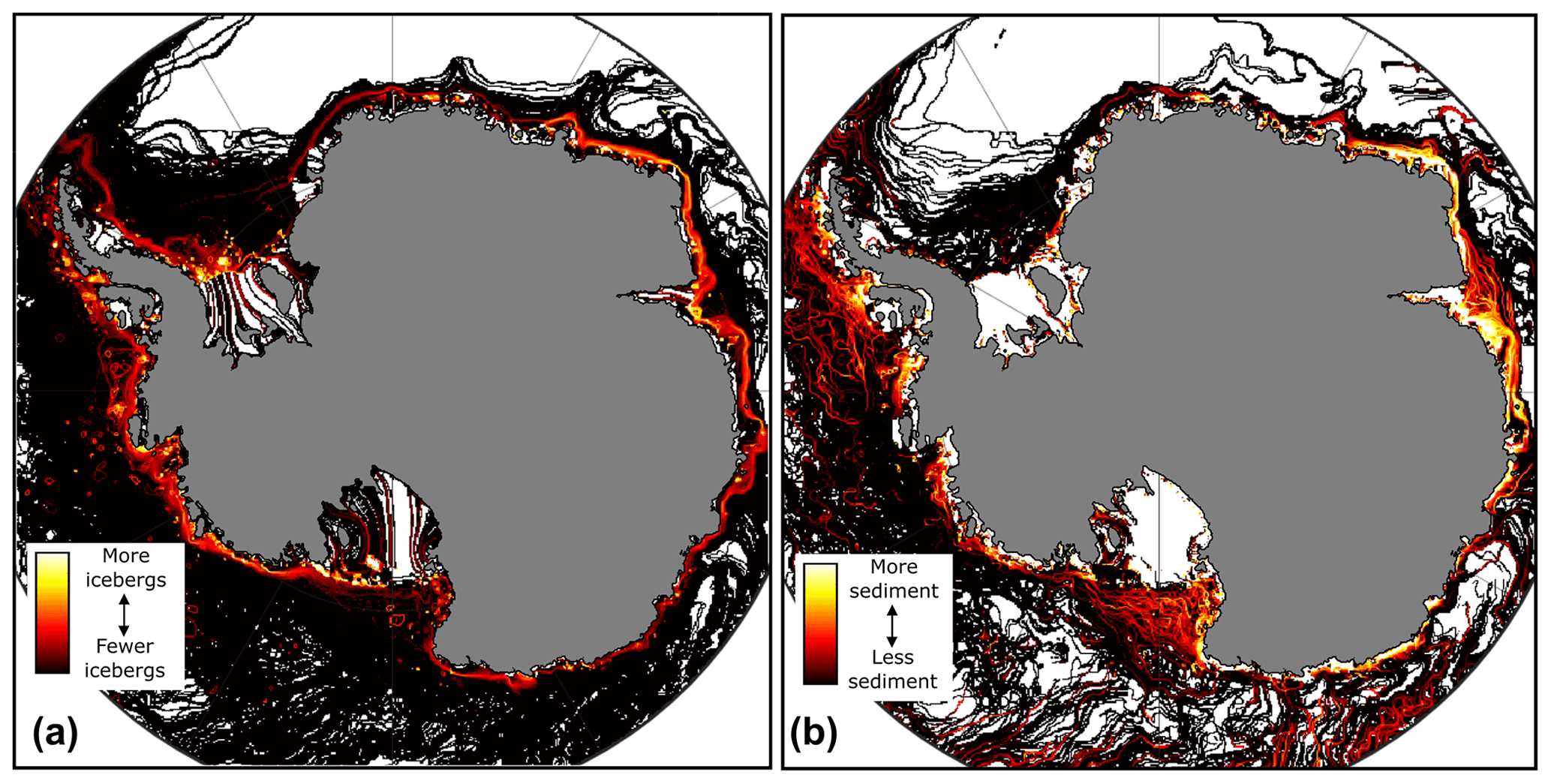
Figure 7 (a) Heatmap of ocean surface velocity paths, which are assumed to approximate iceberg paths. “Hotter” colours highlight areas where icebergs pass through more frequently. (b) The relative quantity of iceberg-rafted sediment deposited by our representation of icebergs (unitless). The broad pattern of iceberg movement produced by our algorithm compares favorably with modelled iceberg trajectories accounting for additional influences such as wind velocities and sea ice (Rackow et al., 2017, their Fig. 2), as well as observed trajectories of large (>5 km across) icebergs from the U.S. National Ice Centre and Brigham Young University (Stuart and Long, 2011; presented in Tournadre et al., 2016, their Fig. 9).

We verify that our iceberg pathways are traced broadly correctly by comparison to observations of iceberg movement. Our results are broadly similar to observed iceberg tracks and studies modelling iceberg drift and distribution (Fig. 7; Stuart and Long, 2011; Rackow et al., 2017). In addition, the spatial distribution of smaller icebergs observed from ships matches with the distribution we produce (Orheim et al., 2021). Trajectories are not consistent from ∼90° E westward to ∼60° W because the path of the Antarctic Coastal Current strays outside of our model domain (and study area) at ∼90° E (Fig. 7). A larger domain would therefore be required to study areas between 90° E and 60° W (e.g. Iceberg Alley in the Weddell–Scotia confluence).

Due to very sparse in situ measurements, knowledge of bottom current flow around ice sheets is mainly derived from shallower oceanographic data, but we suggest the ORAS5 ocean reanalysis product provides the best estimate available. The data used span 24 months (2018–2019).

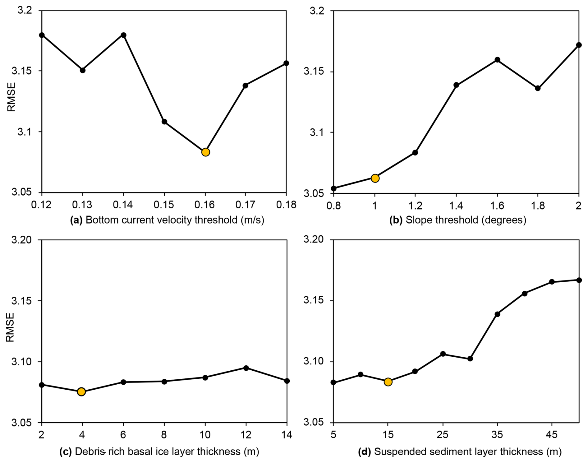
Figure 8 Best estimate root-mean-square error (RMSE) results of tuning (a) bottom current erosion threshold, (b) slope threshold, (c) debris-rich basal ice layer thickness and (d) suspended sediment layer thickness parameters. The parameter value selected is highlighted in yellow. Experiments were conducted using initial assumptions of a 1.2° slope threshold, 0.16 m s⁻¹ bottom current velocity threshold, 6 m basal ice thickness and 15 m suspended sediment layer thickness.

3.2 Parameter tuning and sensitivity tests

Estimating the provenance of debris generated beneath the ice and transported in the ocean requires assumptions regarding, and simplifications of, a highly complex and often poorly understood series of systems. We explore parameter sensitivity and tune the most poorly constrained parameters used. This is done by comparing the TASP prediction to seafloor surface sediments and calculating the root-mean-square error (RMSE) and coefficient of determination (R²). We note that no parameter tested was able to change the RMSE by more than ∼10 % (Fig. 8). This suggests the input ε_Nd map is likely the major source of discrepancies between TASP's results and measured seafloor surface sediments. Here, we do not formally explore parameter interdependence and recommend that TASP users explore the model parameter space for their own use cases.

For the terrestrial component, experiments were performed with spatially variable k (“quarrying” coefficient) values for different ice drainage basins, as in Pollard and DeConto (2019). However, this revealed a negligible impact on results. This is most likely because the map of k used only varied over very large-scale basins (Pollard and DeConto, 2019). A finer resolution, lithology-based estimate of “erodibility” might lead to different rock types being represented to greater and lesser extents offshore, improving the accuracy of modelled provenance signatures.

Firstly, experiments varying the thicknesses of the debris-rich basal ice layer were run (Fig. 8c). This parameter was varied between 2 and 14 m, in line with the observed range of thicknesses (Gow et al., 1979; Christoffersen et al., 2010; Shaw et al., 2011; Pettit et al., 2014) and results compared with seafloor surface sediment data. This revealed that the overall result is relatively insensitive to the chosen basal debris-rich ice layer thickness, with an optimal value of 4 m (Fig. 8c).

The amount of englacial debris relative to the basal debris concentration is another poorly constrained parameter. It was by default set to 10⁻⁵ times the maximum debris load at the base of the ice column based on Dowdeswell and Murray (1990), but experiments were conducted varying it between 10⁻⁶ and 10⁻³. These results revealed TASP is insensitive to this parameter, although excluding this englacial debris entirely (i.e. setting the relative concentration to 0) does have a significant impact on the results (Fig. 9).

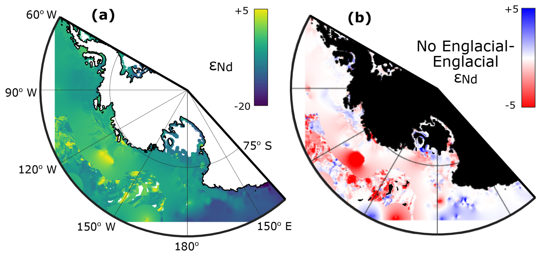
Figure 9 Impact of assuming all debris is contained in a basal layer. (a) The result assuming there is no englacial debris. White areas offshore lack data. (b) Difference between the best match estimate ε_Nd values assuming englacial debris is absent (a) or present (Fig. 11g). Black offshore areas lack data.

The sediment transport method selected at a given seafloor location will be influenced by the thresholds used to determine where marine transport mechanisms are active, i.e. the slope threshold for gravity flows and the velocity threshold at which bottom currents can transport sediment. Given this importance, these parameters were varied over a range of feasible values (Fig. 8a and b). These results show that a velocity threshold of 0.16 m s⁻¹ and slope threshold of 1.0° produce the optimal results.

The treatment of bottom currents described in Sect. 2.3 requires estimates of several parameters, including the bottom current threshold required to resuspend sediment, the relationship between mean and peak bottom current velocities, critical depositional stress and roughness length. Most of these parameters can be estimated with some degree of accuracy based on theory and/or empirical data, but the suspended particle layer thickness is subject to significant uncertainty. This is because particles are unlikely to exist as a layer with a clearly defined upper surface. The thickness of the nepheloid layer on the Antarctic margin varies between less than 10 and ∼10²–10³ m (e.g. Tucholke, 1977; Gilbert et al., 1998; Gardner et al., 2018). This parameter was therefore tuned against seafloor surface sediment ε_Nd value measurements (Fig. 8d). Note that this effectively tunes the other constants used in Eqs. (7)–(10).

Very thin suspended particle layer thicknesses (≤5 m) led to very short transport distances, which are unlikely to capture bottom current transport. Using an increasingly thick suspended layer thickness resulted in transport over longer distances, but a poorer match with seafloor surface sediment measurements (i.e. higher RMSE; Fig. 8d). A 15 m layer thickness was therefore used as a compromise, achieving some transport without significantly worsening the match with seafloor surface sediment measurements. Although 15 m is less than the thickness of the nepheloid layer in several sectors of the Antarctic margin (Gardner et al., 2018), we argue it is physically plausible given that nepheloid layer thicknesses there have been measured in austral spring–summer, when the nepheloid layer probably contained remnants of plankton blooms that took place just prior to these measurements. Furthermore, suspended particle concentrations are not uniform and are highest nearest the seafloor, and we are only concerned with bottom currents, which only comprise the lowermost part of the water column. Transmissometer data also suggest that suspended sediment concentrations increase markedly in the lower tens of metres of the water column (Tucholke, 1977; Gilbert et al., 1998; Gardner et al., 2020).

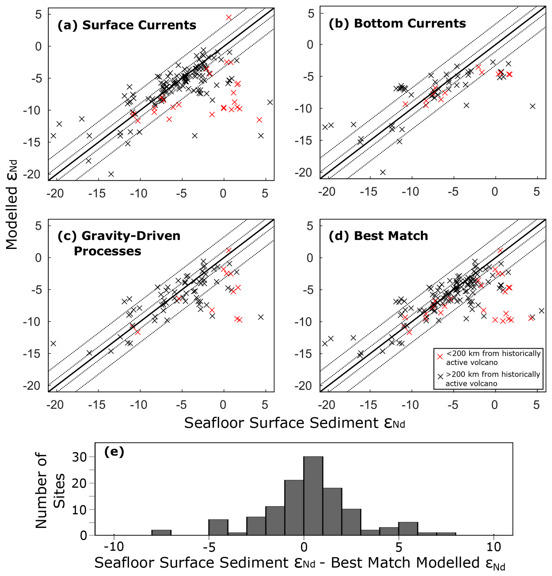
Figure 10 Comparison between observed and modelled ε_Nd values in seafloor surface sediments. Results are shown individually for each transport mechanism of glaciogenic detritus in the marine realm (a–c), plus selection of the best matching method (d). The solid 1:1 line is flanked by dotted lines indicating 1 and 3 epsilon unit deviations, respectively. Red crosses mark samples within 200 km of volcanoes that have been active in the historical observational era. These samples may (or may not) be influenced by volcanic material with a high ($\sim +\mathrm{5}$) ε_Nd value. The difference between the measured and modelled (best match) ε_Nd values of seafloor surface sediments (d) is also shown as a histogram (e).

Figure 11 Simulated ε_Nd values around the West Antarctic margin including the absolute values (a, c, e, g) and difference from the seafloor surface sediment data interpolation (b, d, f, h). The predicted ε_Nd provenance of seafloor surface sediments by modelled surface current (a, b), bottom current (c, d) and gravitational downslope (e, f) transport are shown, as is the best estimate (g, h).

3.3 Comparison to seafloor surface sediment measurements

TASP's results can be compared to the observed ε_Nd values of seafloor surface sediments to evaluate the accuracy of the algorithm (Figs. 10 and 11). This produces a map of ε_Nd values where the most radiogenic (least negative) values are found around the Antarctic Peninsula and along the Marie Byrd Land coast (Fig. 11g). Slightly less radiogenic values are found in the Bellingshausen and Ross seas. The East Antarctic coastline offshore of George V Land produces the least radiogenic values, although the influence of more radiogenic debris transported from the east is clear (Fig. 11g). This general pattern agrees well with surface sediment sample measurements (Fig. 5a), with an overall RMSE of 3.05 and R² of 0.580. We suggest that uncertainty in underlying geology (Appendix A) is the main source of this discrepancy.

TASP's predicted ε_Nd values match 43 % of surface sediment values within 1 epsilon unit and 81 % within 3 epsilon units. The ε_Nd signals in sediment provenance records off East Antarctica and in the Ross Sea exceed 3 epsilon units (e.g. Cook et al., 2013; Wilson et al., 2018; Marschalek et al., 2021). We achieve a close match to surface sediments from specific core sites with down-core records, including International Ocean Discovery Program Site U1521 (Marschalek et al., 2021; measured = −7.7; TASP prediction = −8.0), Integrated Ocean Drilling Program Site U1361 (Cook et al., 2013; measured = −11.5; TASP prediction = −13.3) and Site PS58/254 (Simões Pereira, 2018; measured = −3.0; TASP prediction −3.7). TASP can therefore reproduce observed seafloor surface sediment ε_Nd values to a sufficient degree of accuracy to provide useful predictions of past ice sheet configurations.

Regionally, model–data match is particularly good and nearly always deviates by less than 1 ε_Nd unit in the central Ross Sea and the Bellingshausen Sea (Fig. 11h). TASP also performs better in deep-water locations than for continental shelf sites. Furthermore, the Amundsen Sea embayment offers a dense offshore sample network to compare TASP's results to Simões Pereira et al. (2018, 2020; Fig. 5). The modelled ε_Nd values do not resolve finer-scale provenance features, but the match is good close to the terminus of both Pine Island and Thwaites glaciers and in the central Pine Island–Thwaites palaeo-ice-stream trough (Fig. 11). TASP also broadly captures the mixing of the distinct detritus supplied by each of these two major WAIS outlets (Simões Pereira et al., 2020).

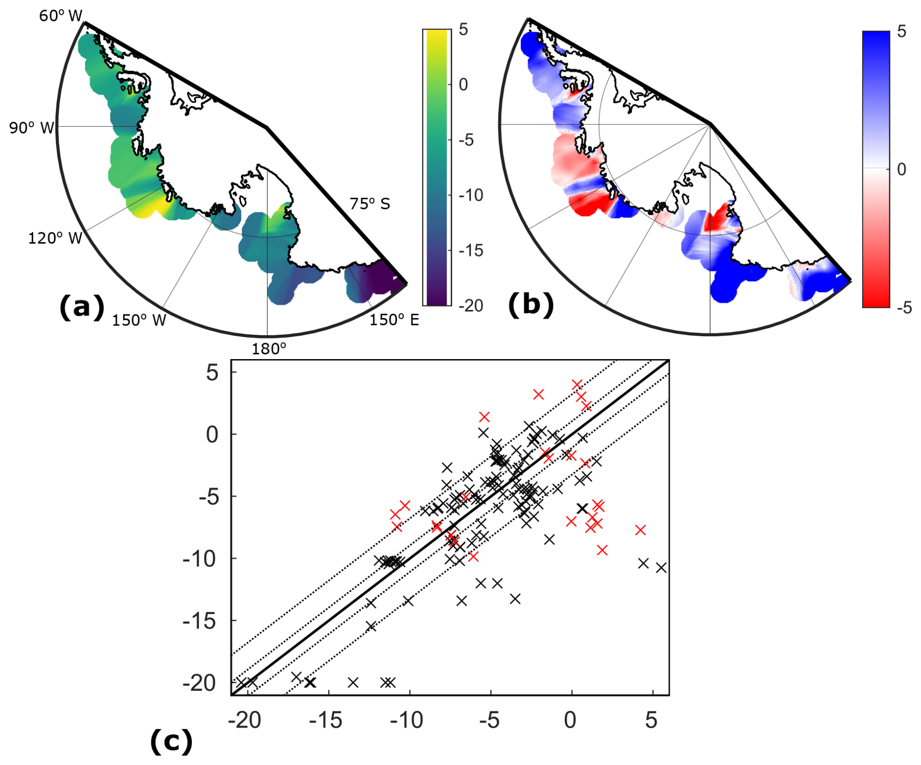
Figure 12 Results when using inverse distance weighting from the ice sheet margin for predicting ε_Nd values of seafloor surface sediments, including (a) the extrapolated ε_Nd values and (b) the difference between ε_Nd values predicted by this method and those measured on the surface sediments. Panel (c) shows the scattered relationship between measured and modelled seafloor surface sediments.

If marine transport processes are neglected, offshore provenance signatures can be estimated from the subglacial component alone (Sect. 2.1). To investigate TASP's performance compared to assuming that debris is simply advected approximately perpendicular to the coast, an inverse distance weighting interpolation was used to extrapolate the provenance signature of the glaciogenic detritus supplied to the ice sheet margin offshore (Fig. 12). The number of neighbours (16) and distance weight (1) were tuned to optimise results. This resulted in a RMSE of 3.70, worse than TASP's prediction incorporating marine processes (RMSE = 3.05) even when considering the full range in parameter choice within the range of plausible values, for which the RMSE remained below 3.19 (Fig. 8). TASP's incorporation of marine detrital particle transport mechanisms therefore results in a closer match to ε_Nd values at seafloor sample sites. This is because an inverse distance weighting method does not reflect transport of detritus approximately parallel to the coast by ocean currents and icebergs.

4 Discussion

4.1 Distribution of different sediment transport processes

An output of TASP's approach is a map showing the regions where surface currents, bottom currents or gravity flows are expected to be the primary debris transport mechanism to a given point on the seafloor (Fig. 13). On parts of the continental shelf, low bottom current velocities mean the surface current estimate often provides the only estimate of ε_Nd values (Fig. 13). The results for the Amundsen Sea and eastern Ross Sea continental shelf suggest a particularly strong influence of surface currents and/or IBRD on the provenance of the sediments deposited in these regions.

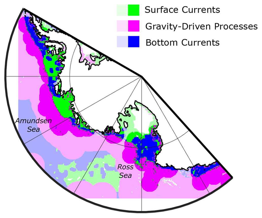
Figure 13 Transport mechanisms for glaciomarine detritus selected for the best estimate ε_Nd value map. Colours are intense within 200 km of seafloor surface sample ε_Nd constraints and pale away from these constraints. White areas indicate grounded ice or a lack of sedimentation. Small black areas away from the grounding line denote where two or more methods predict an identical ε_Nd value.

The threshold for bottom current influence on fine-grained sediment provenance is reached in many locations on the continental shelf and parts of the continental slope and rise (Fig. 13). These areas are particularly concentrated along the western Ross Sea continental shelf, Antarctic Peninsula, Marie Byrd Land coast, Victoria Land coast and George V Land coast. In the Ross Sea, this may reflect sediment transport along Ross Sea Bottom Water export pathways (Orsi and Wiederwohl, 2009).

Beyond the continental shelf, gravitational downslope processes dominate in nearly all locations (Fig. 13). Compared to the other sediment transport mechanisms, sediment core sites in these regions typically provide the closest match with TASP's predictions, with an RMSE of 3.20 (Figs. 10 and 11). Substantial model–data mismatch for the gravitational downslope mechanism is limited to sites with special, localised environmental settings, which are discussed in detail below (Sect. 4.3). The close agreement between TASP and the measured seafloor surface sediments suggests that sediment transport perpendicular to the shelf break is dominant further offshore and that the amount of detritus moved by gravitational downslope processes typically exceeds that of detritus solely supplied by ocean currents in these areas.

4.2 Volcanic detritus

Windblown dust from other continents reaches Antarctica and could influence the provenance signature of marine sediments (Neff and Bertler, 2015), particularly during full glacial periods (e.g. Sugden et al., 2009). However, such sources are minor in most Antarctic continental margin settings used for sediment provenance studies (e.g. Walter et al., 2000; Wengler et al., 2019) and are therefore neglected.

However, volcanic material and tephra erupted above the ice surface and carried offshore, either by wind, in layers within icebergs or on sea ice, could be present in the seafloor surface sediments in areas close to and downwind of volcanoes (e.g. Chewings et al., 2014). This detritus could substantially influence ε_Nd values, as Cenozoic volcanic material in West Antarctica and Victoria Land is highly radiogenic ($\sim +\mathrm{5}{\mathit{\epsilon }}_{\mathrm{Nd}}$) and has a high Nd concentration (Goldich et al., 1975; Aviado et al., 2015; Futa and LeMasurier, 1983; Hart et al., 1997). TASP does not attempt to account for the influence of this volcanic material. Indeed, areas where predicted ε_Nd values are less radiogenic (lower) than those observed include the coast of Victoria Land, part of the Hobbs Coast of Marie Byrd Land and the area around the northern tip of the Antarctic Peninsula (Fig. 11). This mismatch is likely attributable to volcanoes in these areas that are either still active or have been active in the recent past (e.g. Dunbar et al., 2021; Patrick and Smellie, 2013; Fig. 5). The explanation for mismatch in these areas is supported by evidence from grain size distributions and visual observations (Kellogg et al., 1990; Atkins and Dunbar, 2009), as well as clay mineralogy (e.g. Hillenbrand and Ehrmann, 2005; Hillenbrand et al., 2021; Wang et al., 2022), indicating that volcanic detritus forms a significant component of the sediments near these active volcanic provinces. Neodymium isotope records from these areas should therefore be interpreted with caution.

Three samples collected adjacent to the Adare and Hallett peninsulas on the northern Victoria Land coast recorded particularly radiogenic ε_Nd values that are also not captured by TASP (outliers in Fig. 10; Table A2). Visual mineralogical composition and ε_Nd values of $>+\mathrm{4}$ suggest they consist almost entirely of detritus derived from the late Cenozoic volcanic rocks constituting these peninsulas. However, as the source volcanoes have not been active for at least ∼2 million years (LeMasurier et al., 1990), this discrepancy cannot be attributed to recent tephra deposition but must result from the supply of locally eroded volcanic material. These results instead highlight a limitation of our 10 km model resolution, which is not able to resolve such localised areas of a particular rock type (Fig. 5). If such sites close to the shore were of interest for sediment provenance tracing, a more localised, higher-resolution modelling approach would need to be pursued to yield more accurate results.

To visualise the locations of seafloor surface sediment samples that are in the vicinity of recently active volcanoes and therefore potentially influenced by significant volcanic deposition, sites within 200 km are highlighted in red in our scatter plots and excluded from our statistics (Fig. 10). This distance was chosen based on visual inspection of areas of obvious discrepancy with seafloor surface sediment measurements (Fig. 11). We emphasise that the exclusion of these sites does not imply that sediment provenance data here are not useful; instead, the provenance data in these areas are viewed as having the potential for unaccounted for volcanic influences. One exception is the recent volcanic activity suggested in the Hudson Mountains near Pine Island Bay in the eastern Amundsen Sea embayment (Patrick and Smellie, 2013; Corr and Vaughan, 2008), which we do not use to exclude data. Any volcanic input to marine sediments here is likely very local and minor given both the restricted geographical distribution of this tephra on land (Corr and Vaughan, 2008) and the rare and locally restricted occurrence of tephra in marine sediments from the area (Herbert et al., 2023).

Volcanogenic detritus could also reach sample sites from volcanic seamounts and islands (Fig. 5b). These are widely distributed and range in age from the early Cenozoic to recent (Johnson et al., 1982; Prestvik and Duncan, 1991; Hagen et al., 1998; Hagedorn et al., 2007; Panter and Castillo, 2007; Rilling et al., 2009; Lawver et al., 2012; Kipf et al., 2014), with radiogenic isotope compositions that are similar to other Cenozoic volcanic rocks (Kipf et al., 2014; Panter and Castillo, 2007; Prestvik and Duncan, 1991). These seamounts and islands are not accounted for in TASP's predicted ε_Nd values for seafloor surface sediments as the spatial extent and magnitude of the influence of such features is uncertain.

4.3 Localised impact of grounded icebergs and sea ice

Offshore of the Wilkes Subglacial Basin and adjacent to the King Edward VII Peninsula, predicted ε_Nd values are more radiogenic (higher) than those measured in the seabed sediments (Fig. 11). A key factor influencing ε_Nd values in these regions is the supply of relatively radiogenic detritus via the westward-flowing Antarctic Coastal Current, which in both these areas appears to deliver a greater fraction of radiogenic detritus in our model than in the real world. This is most likely a consequence of icebergs remaining closer to the coast in the simulation compared to reality. In these areas, we suggest that the ocean reanalysis product may not be resolving local factors – such as local ocean currents and the presence of grounded icebergs and fast ice – which lead to more far-travelled icebergs carrying relatively radiogenic detritus being diverted north away from the coast. Offshore from Wilkes Subglacial Basin, for example, high-resolution modelling of sea ice trajectories around the Mertz Glacier area shows that icebergs coming from the east are deflected north by a mélange of fast ice and grounded icebergs (Marsland et al., 2004), allowing locally derived debris (with more negative ε_Nd values) to be more dominant in the lee side of this “promontory” (Orejola et al., 2014). This area of deflection matches well with the area where TASP's results and observations differ (red and blue areas in Fig. 14). Similarly, a gyre offshore from King Edward VII Peninsula deflects icebergs, which drift within the Antarctic Coastal Current westwards along the Amundsen Sea shelf, to the north before injecting them into the eastward-flowing Antarctic Circumpolar Current (Rackow et al., 2017). This implies that grounded bergs, sea ice and unresolved ocean currents are a key control on the provenance of continental shelf sediments in these regions and should be carefully considered when interpreting sediment provenance records.

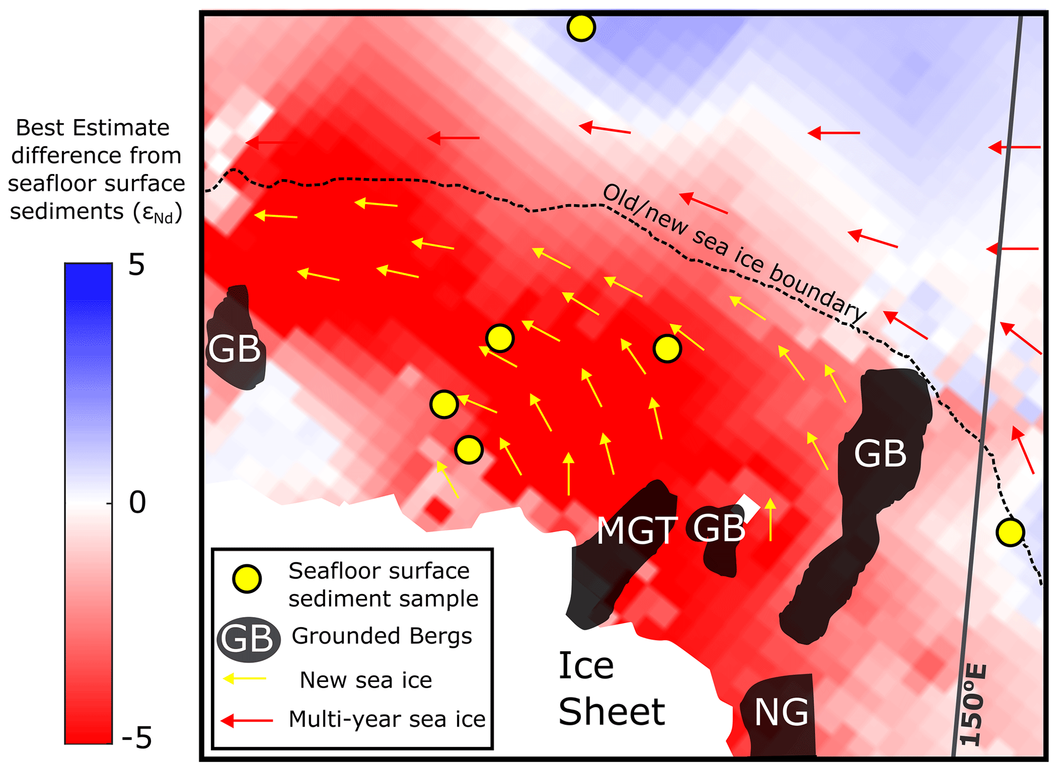
Figure 14 Close-up of the Mertz Glacier Tongue (MGT) region imaged in June 1999, adapted from Massom et al. (2001) and Marsland et al. (2004). Location of map shown in Fig. A1. Red and blue colours indicate the discrepancy between the modelled and core top ε_Nd values as in Fig. 11h. Overlain is a map of old (multi-year) and new sea ice trajectories (red and yellow arrows, respectively), which are deflected to the north due to grounded bergs (GB) and fast ice. Note that the MGT had undergone a major calving event in 2010, but since then another seaward-extending tongue consisting of floating glacial ice protruding from Ninnis Glacier (NG) and Mertz Glacier and amalgamated by fast ice has been established (e.g. Wang et al., 2018). Seafloor surface sample measurement locations are shown in yellow.

At some sites, observed mismatch may also be linked to uncertain dating of seafloor surface sediments. To achieve a good spatial coverage, we group all available measurements on samples likely to be late Holocene to modern in age, but difficulties in radiocarbon dating of often carbonate-free Antarctic sediments mean these samples may vary in age throughout the Holocene on a site-by-site basis.

5 Conclusions and future direction

We present TASP, the first algorithm to predict offshore sediment provenance using the results of ice sheet modelling and ocean modelling. Debris is incorporated and routed at the ice sheet bed based on ice sheet model results and an erosion law. Marine detrital particle transport mechanisms include representations of surface currents, which are used to approximate iceberg trajectories. Bottom currents redistribute sediment if a velocity threshold is reached, and gravity flows transport material downslope. These estimates are then used to make a provenance proxy map across the seafloor, thereby directly predicting sediment core data for a given modelled ice sheet extent.

To demonstrate that TASP produces useful results, it is applied to estimate Nd isotope compositions around West Antarctica and the East Antarctic George V Land margin. Comparison of our results to seafloor surface sediment measurements show that most (81 %) core sites differ by less than 3 epsilon units, which is less than the signal typically seen in down-core records. This application of TASP to modern Antarctic Nd isotope compositions also helps understand the modern sedimentary system. For instance, our findings show that westward-flowing ocean currents control deposition on the continental shelf, while a good model–data match in deeper waters indicates gravity-driven processes are the dominant sediment delivery mechanism there. Furthermore, our results help suggest regions where local factors such as geological uncertainty, recent volcanism or sea ice are likely impacting present-day deposition, with implications for interpreting sediment provenance data in these locations. The TASP algorithm is particularly powerful beyond the continental shelf, where it produces a close match when using a simulation of the modern ice sheet to predict ε_Nd values of seafloor surface sediments. This is likely because greater integration of provenance signals makes our approach less reliant on precise mapping of uncertain subglacial geology.

The development of TASP as presented here will permit future application to palaeo ice sheet model simulations. Model output from smaller-than-present ice sheets can be directly input to the framework provided here, although use of high-resolution modelled palaeo ocean currents would be highly beneficial. Results from applying TASP this way will help interpret existing and new sediment provenance records by suggesting what ice sheet configurations could produce the changes in ε_Nd values (and potentially other provenance proxies) recorded at any given core site. Tighter coupling of numerical ice sheet model simulations and provenance data offers the potential for the advancement of both fields; results of numerical modelling can be directly compared to real-world constraints, and interpretations of geochemical and mineralogical data can be tested, visualised and quantified in terms of ice sheet volume and extent. TASP also has the potential to better target potential sediment core sites for provenance studies, as the regions with the greatest sensitivity to a provenance proxy can be identified.

Improved knowledge of subglacial geology, particularly in the West Antarctic interior, would enable TASP to produce even more useful and accurate results. Future geophysical surveys, as well as drilling campaigns targeting subglacial sediments and bedrock, will reduce uncertainty in our ε_Nd map and thus predictions offshore. Additional insights could be achieved by expanding our Antarctic case study to different parts of the Antarctic continent. Our method could also be adapted for numerous provenance proxies, such as detrital mineral dating, major and trace element geochemistry, clay and heavy mineralogy, or clast petrography. Each of these proxies offers a different sensitivity to changes in erosion patterns and thus different precision and insights in different regions and at different times in the past (Licht and Hemming, 2017).

Appendix A: Regional description of the neodymium isotope composition map

A1 Approach

Here we present a region-by-region summary of the sources used to define the extent and Nd isotope composition of the bedrock of West Antarctica and adjacent areas of East Antarctica. A description of geological formations, lithologies and the tectonic framework of the study area is not relevant to this study, and therefore it is not discussed here. For reviews of East Antarctic, West Antarctic and Transantarctic Mountain geology, see Boger (2011), Jordan et al. (2020) and Goodge (2020), respectively.

The ε_Nd value map (Fig. 5a) was based on measurements of rock ε_Nd values from published literature sources that had been previously compiled (Simões Pereira et al., 2018, 2020; Marschalek et al., 2021). These datasets were extended across the domain used here. Where coordinates for the locations of rock samples were not given in the original publication, they were taken from the SCAR Antarctic Digital Database Map Viewer (https://www.add.scar.org/, last access: July 2022) based on the location name.

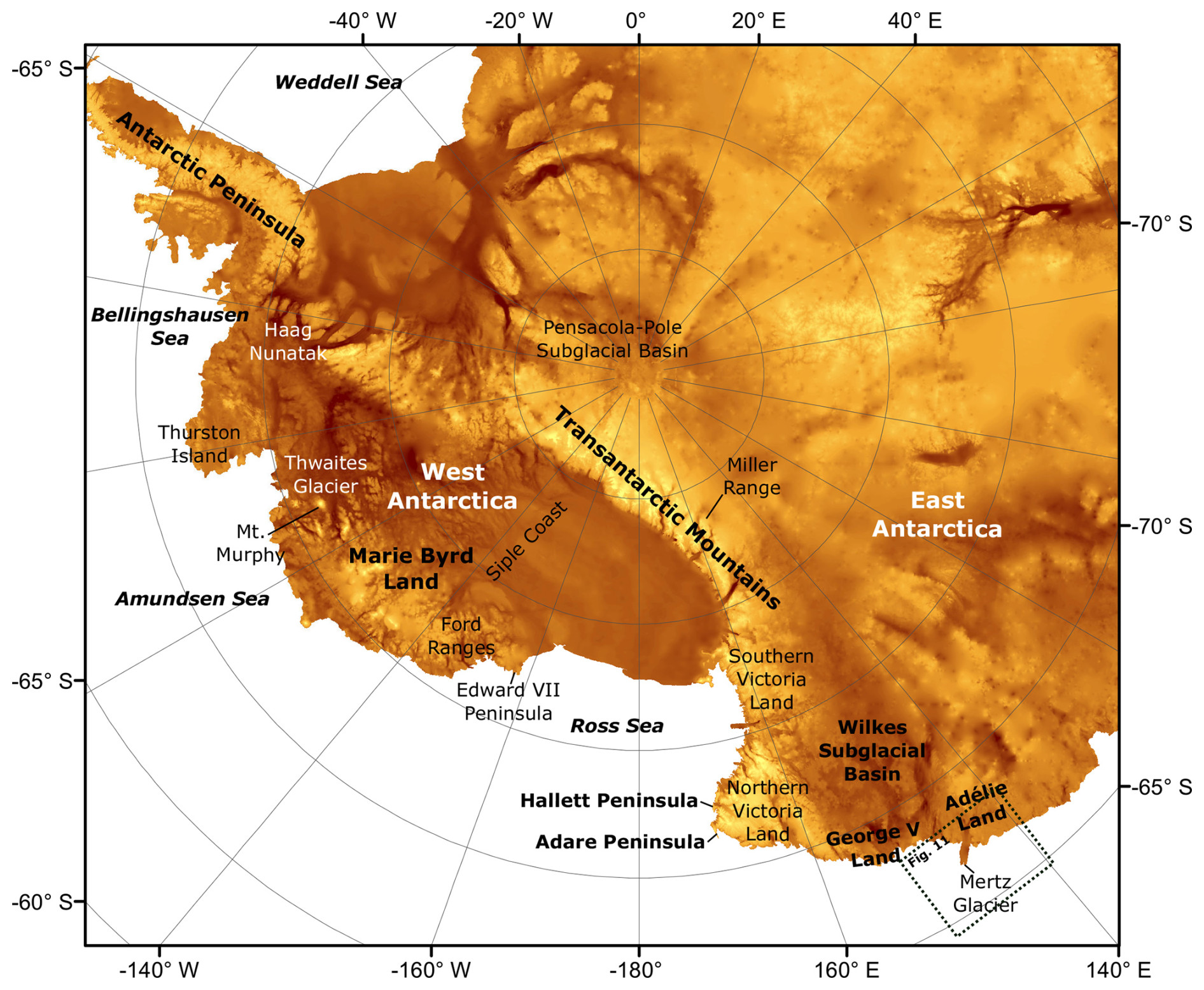
Figure A1 Geographical locations mentioned in the Supplement and main text displayed on BedMachine topography (Morlighem et al., 2020). The area covered by the map shown in Fig. 11 is marked by the box with the dotted black outline.

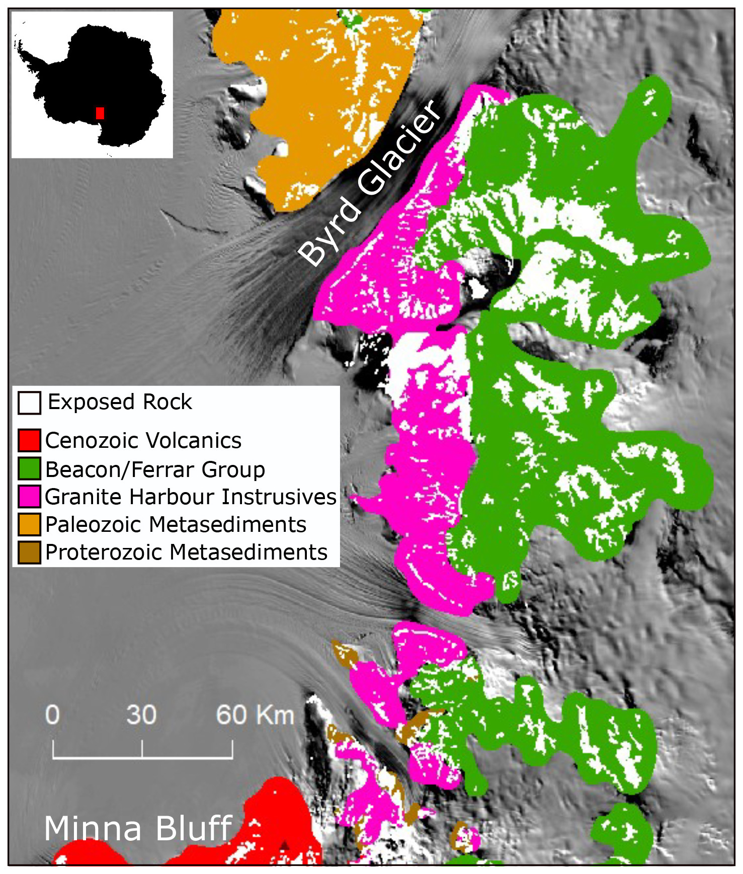
Figure A2 Example of the high-resolution rock polygons from GeoMAP (white; Cox et al., 2023) vs. the simplified polygons used to construct the ε_Nd value map (coloured). The latter are better suited to the $>\sim \mathrm{10}$ km resolution of interest here. The region shown is a section of the Transantarctic Mountains between Byrd Glacier and Minna Bluff. The geology is overlain on MODIS imagery (Haran et al., 2014, updated 2019). The location within Antarctica is indicated in the inset on the upper-left side.

To convert these literature “point data” into a continuous map, outcropping rocks were grouped. This was facilitated by the recent digital geological mapping of Antarctica from the SCAR GeoMAP project (Cox et al., 2023). To simplify this map, which comprised polygons at a resolution far beyond that required for this study, adjacent outcrops were grouped where subglacial continuity between exposures was deemed reasonable (see example in Fig. A2). For each major rock type, the point ε_Nd values were then interpolated and masked to the area of the simplified polygons. A resolution of 10 km was used, which is sufficient given the uncertainties resulting from the ice cover and matches the resolution used in the ice sheet model. These areas of exposed rock can be considered as having a high level of confidence in the final map, particularly when ε_Nd values for the outcropping rock group have been measured at numerous localities.

Most of the study area is covered by ice, making direct geological observations impossible. Pertinent airborne and on-ice geophysical (i.e. gravity, magnetic and subglacial geomorphology obtained by radar) studies were therefore used to inform ε_Nd values beneath the ice by making interpretations regarding the subglacial geology (e.g. Jordan et al., 2013a; Goodge and Finn, 2010; Studinger et al., 2006; van Wyk de Vries et al., 2018; Paxman et al., 2019). In some regions, this approach can produce reasonably robust inferences. However, in other areas, relationships between exposed and subglacial geology are more obscure. Even in areas where geophysical constraints are good, the subglacial bedrock there may be hundreds (or thousands) of kilometres away from the nearest comparable outcropping rocks. Consequently, using interpolation from the nearest outcrops to assign ε_Nd values, as described above for exposed rocks, could lead to bias towards only the geographically nearest measurement. Interpolation may therefore fail to reflect the true variability of the subglacial geology in such areas. To avoid this, areas where a subglacial rock type was predominantly “geophysically” defined were uniformly assigned a mean ε_Nd value based on all suitable measurements of the rock type.

The sources used to determine the extent of subglacial geology and to estimate the ε_Nd value for each rock group are discussed in detail below. To keep the initial offshore ε_Nd value estimate as independent as possible, an inverse approach was specifically avoided when constructing the subglacial ε_Nd map (i.e. using offshore values to predict onshore ones). In a few locations where virtually no geophysical or geological data were available, unconsolidated sediment samples from subglacial sediment coring (Farmer et al., 2006) were used to estimate the isotopic composition upstream. A formal inversion for subglacial geochemistry, similar to that recently applied to fluvial provenance (Lipp et al., 2020), would undoubtedly provide a much-improved match with modern observations and insights into subglacial geology to apply to simulations of past ice sheets. However, further development would be required to implement a formal inverse approach in a glacial setting, as additional information beyond an offshore measurement near the ice sheet margin is required to give structure to interior ε_Nd values and avoid uniform values along a flow line.

To indicate the approximate uncertainty in the map produced, areas are classified with confidence levels 1–4 (Fig. 5b).

1. Confidence level 1 uses exposed rocks (high confidence; black) and is applied for exposed rock with ε_Nd data. The quantity and spatial distribution of ε_Nd measurements varies between rock types, and in some instances sparse data meant that the number of data points used in the interpolation across a rock group was low.

2. Confidence level 2 uses geophysical constraints (moderate confidence; brown) and is applied in areas with subglacial geology constrained by gravimetric, magnetic, geomorphological, etc., data. Epsilon Nd values inferred for rock groups are based on the nearest equivalent exposures, but ε_Nd values may be different away from the rock outcrop with ε_Nd data, or certain rock groups may be over- or under-represented. For instance, outcrops of Neogene volcanic rocks dominate in Marie Byrd Land, but Palaeozoic basement and Cretaceous plutonic rocks are much more widespread (e.g. Rocchi et al., 2006).

3. Confidence level 3 uses sedimentary constraints (low confidence; light grey) and is applied in areas with few direct constraints that are limited to isolated subglacial samples obtained by drilling through the ice. Epsilon Nd values are determined from these limited samples interpreted in the context of surrounding rock exposures.

4. Confidence level 4 indicates that no estimate was made (white) as these areas are without any rock type constraints and are filled using Kriging.

Different rock types have different concentrations of Nd, meaning some rock types will contribute disproportionately to the ε_Nd values of subglacial detritus. This effect is not accounted for here due to the uncertainty in Nd concentrations of different rock types, making quantitative assessments challenging. Assuming constant Nd concentrations still yields useful results, but the inclusion of variable concentrations in future work would improve the accuracy of our results. Our approach also neglects any pre-glacial sedimentary strata, marine and other sediments deposited when ice sheets were more retreated than today (e.g. under the WAIS and the Wilkes Land–Adélie Land sectors of the East Antarctic Ice Sheet) or allochthonous subglacial till overlying in situ bedrock at the base of grounded ice. However, subglacial mixing of detritus is to some degree accounted for by the interpolation of ε_Nd values between regions with assigned ε_Nd values, as well as assumptions of mean ε_Nd values of the surrounding rock types in regions where pre-glacial and marine sedimentary strata or till sheets are likely present under the ice. These simplifications have the effect of smoothing the bedrock ε_Nd values. Fully accounting for reworking of subglacial sediments would require a full integration of ε_Nd values in time-evolving ice sheet model runs.

Some regions – particularly the interior of the WAIS towards Marie Byrd Land, the southernmost Transantarctic Mountains and the hinterland of the Bellingshausen Sea – lack reliable geophysical constraints. In these regions, initial estimates were made by simply interpolating the map produced over the remaining gaps. However, this led to some obvious discrepancies between the ε_Nd values of rocks on land and coastal marine sediments. This effect was particularly pronounced in regions of West Antarctica, where geophysical bedrock studies typically focus on detecting comparatively radiogenic subglacial igneous bodies. The lack of constraint on surrounding rock biases ε_Nd values. To account for this, most large areas of the study area with unassigned ε_Nd values were prescribed a value informed by sparse subglacial till samples (e.g. Farmer et al., 2006) and surrounding rock types, which markedly improved agreement with marine surface sediment ε_Nd values. As spatial variability in ε_Nd values is unknown in these regions, the assigned ε_Nd values were assumed to be uniform.

A2 George V Land and the Wilkes Subglacial Basin

The extent of pre-Cambrian East Antarctic rocks is mapped according to Goodge and Finn (2010), which is broadly consistent with ADMAP2 magnetic anomalies (Golynsky et al., 2018). The coastal extent of these pre-Cambrian rocks is based on interpretation of these data in Bertram et al. (2018). Limited measurements of this rock group give spatially variable ε_Nd values, spanning approximately −33 to −11 in the Miller Range of the central Transantarctic Mountains (Borg et al., 1990; Borg and DePaolo, 1994), −24 to −22 along the Adélie Land coast (Peucat et al., 1999) and −16 to −15 at the bed of the EPICA Dome C ice core (Delmonte et al., 2004). The pre-Cambrian rocks are assigned a uniform ε_Nd value of −20, which is considered reasonable given the limited exposure of these rocks. Beyond the edge of the area studied, no attempt was made to compile literature ε_Nd values as erosion rates are low (e.g. Jamieson et al., 2010; Fig. 6a) and the Antarctic Coastal Current will carry any detritus reaching the coast westwards out of the study area (e.g. Fig. 7). Rocks in other parts of Antarctica are thus unlikely to substantially impact the provenance signature of the regions studied offshore here, although some ice flowlines do cross beyond the edge of the study area. Based on the assumptions described above, the rest of East Antarctica was also assigned a uniform ε_Nd value of −20.

Exposures of the late Neoproterozoic to Ordovician Wilson, Bowers and Robertson Bay terranes are widespread throughout northern Victoria Land. For these three respective rock groups, measured ε_Nd values range from −22.6 to −11.1 (Talarico et al., 1995; Henjes-Kunst and Schussler, 2003; Estrada et al., 2016), −19.9 to −10.5 (Tonarini and Rocchi, 1994; Henjes-Kunst and Schussler, 2003) and −15.6 to −12.3 (Henjes-Kunst and Schussler, 2003). However, most measurements cluster around a mean ε_Nd value of approximately −14, which is assigned uniformly to these groups.

Granite Harbour Intrusive rocks are exposed in Victoria Land, and although these have relatively uniform ε_Nd values with a mean of $\sim -\mathrm{12}$ (Cox et al., 2000; Armienti et al., 1990; Dallai et al., 2003; Rocchi et al., 1998, 2009), their ε_Nd values are allowed to vary spatially in our ε_Nd map. These granitic rocks are also suggested to be present in the Wilkes Subglacial Basin, but the southern and northern extent and depth of these subglacial granitic bodies are subject to significant uncertainty (Ferraccioli et al., 2009).

The youngest rocks in the Wilkes Subglacial Basin are Ferrar Group dolerites and basalts, which intrude and overlay Beacon Supergroup siliciclastic rocks. The extent of these rock types beyond their very limited outcrops is estimated using the previous interpretation of geophysical data in Bertram et al. (2018), with more southern limits mapped according to Jordan et al. (2013a). Jordan et al. (2013a) show a greater extent of Beacon Supergroup and Ferrar Group rocks compared to the interpretations of Studinger et al. (2006) in southern Victoria Land, and we favour this more recent interpretation. Ferrar Group dolerites and basalts are isotopically well constrained and consistent, with mean ε_Nd values of $\sim -\mathrm{6}$ (e.g. Elliot et al., 1999; Hergt et al., 1989; Molzahn et al., 1996). The ε_Nd values in Beacon Supergroup rocks are much more varied and sparsely measured, with mean values around −12 (Fleming, 1995; Bertram, 2018; Marschalek et al., 2021). Given that (i) the relative abundance of these rocks is uncertain, but Ferrar sills are common through the Wilkes Subglacial Basin (Ferraccioli et al., 2009); (ii) concentrations of Nd are approximately twice as high in Ferrar Group rocks than Beacon Supergroup rocks (Bertram, 2018); and (iii) the uppermost Beacon Supergroup rocks have a Ferrar-like isotopic composition (Elliot et al., 2017), we assume an ε_Nd value of −7 is reasonable for a typical mixture detritus originating from Beacon Supergroup and Ferrar Group rocks.

Areas between the coast and the Beacon Supergroup and Ferrar Group rocks are assumed to be a mixture of Lower Palaeozoic rocks (i.e. Wilson Group, Bowers Group, Granite Harbour Intrusive and Robertson Bay Terranes), which are known to be present subglacially based on Miocene sediments recovered at Integrated Ocean Drilling Program (IODP) Expedition 318 Site U1359 (Pandey et al., 2018). Based on the most unradiogenic ε_Nd values measured in nearby seafloor surface sediments ($\sim -\mathrm{15.5}$; Cook et al., 2013), this local endmember may be slightly more unradiogenic than the −14 to −12 described above. We therefore opt for an ε_Nd value of −15 here. Sedimentary basins in the Wilkes Subglacial Basin (Frederick et al., 2016) are ignored, as these are assumed to be comprised of mixtures of relatively local bedrock and are therefore accounted for using mean ε_Nd values for each rock type.

A3 Southern Victoria Land and the Transantarctic Mountains

The central Transantarctic Mountains provide some of the most extensive rock outcrops in Antarctica (Goodge, 2020). Neodymium isotope composition measurements are also plentiful for many rock types, making this a well-constrained region. We use the mapping of Cox et al. (2023) and isotopic data compiled and referenced in Marschalek et al. (2021) to produce the ε_Nd value map here. In the Transantarctic Mountains, there are outcrops of the pre-Cambrian and Beacon Supergroup and Ferrar Group rocks discussed above. Other rock types with ε_Nd measurements include the Neoproterozoic to early Paleozoic metasedimentary Skelton, Byrd, Beardmore and Liv groups (e.g. Borg et al., 1990; Borg and DePaolo, 1994; Cox et al., 2000; Goodge et al., 2008) and the Palaeozoic Granite Harbour Intrusives (e.g. Goodge et al., 2012; Borg et al., 1990; Borg and DePaolo, 1994; Cox et al., 2000).

On the East Antarctic side of the southern Transantarctic Mountains, we extend the Ferrar Group and Beacon Supergroup into the Pensacola-Pole subglacial basin based on interpretations by Paxman et al. (2019). The Precambrian East Antarctic craton, the extent of which is defined by Goodge and Finn (2010), is prescribed an ε_Nd value of −20 as described above. In the area between rock exposures in the southern Transantarctic Mountains and geophysical data around the South Pole, relatively little is known about the subglacial geology due to a lack of data; thus, the gap was initially simply interpolated across. However, predicted ε_Nd values at the ice sheet margin for this portion of the Transantarctic Mountains were consistently too radiogenic ($\sim -\mathrm{5}$) compared to ε_Nd values of recent sediments recovered from beneath Whillans Ice Stream ($\sim -\mathrm{8}$ to −9; Farmer et al., 2006). This may be due to a bias towards exposures of the Granite Harbour Intrusive rocks, which have a mean ε_Nd value of −4.6 (n=10) in this region (Borg et al., 1990; Borg and DePaolo, 1994). These rocks are likely to be more resistant to erosion than the surrounding sedimentary rocks, such as those of the Liv Group and Beacon Supergroup, meaning they may outcrop a disproportionate amount. There may also be bias towards exposure or measurement of more radiogenic beds in the Liv Group (e.g. Wareham et al., 2001).

To combat this bias, we assigned a uniform ε_Nd value of −9 around rock outcrops based on the limited measurements of Beardmore Group and Liv Group metasediments, which likely comprise the bedrock between the Granite Harbour Intrusive batholiths (Marschalek et al., 2021). An ε_Nd value of −9 is also comparable to two measurements of the Beacon Supergroup in the southern Transantarctic Mountains (Marschalek et al., 2021).

To the north, the youngest rocks in this region belong to the Cenozoic McMurdo Volcanic Group in Victoria Land. These are extensively sampled and allowed to vary spatially in our map but are generally consistent with a mean ε_Nd value of $+\mathrm{5.3}\pm \mathrm{0.6}$ (e.g. Aviado et al., 2015; Martin et al., 2013; Phillips et al., 2018).

Table A1 Endmember assignment for central West Antarctica. The term “West Antarctic sediments” refers to our approximation for all sediments likely to underlie the WAIS since the opening of the West Antarctic rift system, including pre-glacial sediments, marine and other sediments deposited during ice-free periods, and subglacial till. It is assumed the surrounding rock types forming the source rocks for these sediment types probably remained the same throughout the Cenozoic.

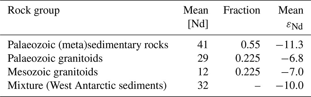
A4 Siple Coast and central West Antarctica

Ice cover is extensive and geophysical data are limited in the West Antarctic interior, making it difficult to constrain the sub-ice geology there. However, till samples from beneath ice streams and in the Ross Sea provide some guidance to the likely subglacial lithologies (Farmer et al., 2006; Licht et al., 2014). Underlying much of this region are subglacial sedimentary basins, which range in age from the opening of the West Antarctic rift system in the mid-Cretaceous through to the Pliocene or Pleistocene (LeMasurier and Landis, 1996). Studies of sediment provenance suggest which rocks may be contributing (Farmer et al., 2006; Licht et al., 2014), including the following kinds of rocks:

• a late plutonic phase of the Ross Orogeny towards the Transantarctic Mountains (i.e. Granite Harbour Intrusives; see references above);

• Cretaceous to Triassic granitic rocks (e.g. Weaver et al., 1992; Craddock et al., 2017; Pankhurst et al., 1998);

• Palaeozoic (meta-)sedimentary rocks such as the Swanson Formation in western Marie Byrd Land and equivalents in the Whitmore Mountains (e.g. Korhonen et al., 2010; Yakymchuk et al., 2015);

• Palaeozoic granitic rocks, such as the Ford Granodiorite in westernmost Marie Byrd Land (e.g. Weaver et al., 1992; Yakymchuk et al., 2015; Korhonen et al., 2010).

Potential mixture of these lithologies in the sedimentary bed based on adjacent exposed rocks suggests an ε_Nd value of $\sim -\mathrm{10}$ (Table A1). This value agrees well with that of the most unradiogenic sediments beneath the Siple Coast ice streams (Bindschadler Ice Stream), and thus it is thought to be representative (Farmer et al., 2006). A uniform ε_Nd value of −10 was therefore assigned to the entire West Antarctic interior. The magnitude and extent of contribution from Granite Harbour Intrusive rocks is difficult to constrain, but as these rocks have a mean ε_Nd value of $\sim -\mathrm{10}$ (Borg et al., 1990; Borg and DePaolo, 1994; Goodge et al., 2012), they may not influence the overall composition very much, and thus they are neglected (Table A1).

It is generally agreed that some Cenozoic volcanic rocks also exist beneath the WAIS. The locations of these Cenozoic volcanic rocks were initially set based on exposed volcanoes, the subglacial volcano inventory of van Wyk de Vries et al. (2018) and the survey of Luyendyk et al. (2003). Preliminary application of the algorithm also found their presence is required to explain sufficiently radiogenic ε_Nd values offshore, assuming surrounding rocks have values of −10 as described above. The extent of these volcanic rocks is subject to some uncertainty (Andrews and LeMasurier, 2021) and volcanic rocks comprise only a small fraction of gravel-sized detritus in the eastern Ross Sea, but it is possible these rocks have been crushed to finer grain sizes by a combination of physical weathering and glacial comminution (Perotti et al., 2017).

Even when these potential volcanic rocks were included, ε_Nd values were not radiogenic enough to match offshore provenance observations. This may be linked to the uniform ε_Nd value of −10 applied for West Antarctic sediment. More radiogenic granitic rocks, potentially similar to the most radiogenic granitoids in the Ford Ranges (Korhonen et al., 2010) or on Thurston Island (Pankhurst et al., 1993), may be widespread in some areas beneath the WAIS, as unexposed Mesozoic-aged rocks are clearly present based on detrital zircon ages (Licht et al., 2014; Marschalek et al., 2021). However, without data to constrain the extent and isotopic composition of these rocks, we favour the addition of extra Cenozoic volcanic rocks to improve the match with observations. Behrendt (2013) correlated magnetic anomalies in the WAIS interior to subglacial late Cenozoic volcanic rocks. We assume that such rocks occur at sites with high magnetic anomalies based on the ADMAP-2 compilation (Golynsky et al., 2018). Although this is a crude approach, new detailed mapping of possible volcanic material or more radiogenic granitic rocks beneath the WAIS is beyond the scope of this study. Indeed, understanding the mixture of rocks beneath the central WAIS would be greatly beneficial for future sediment provenance studies seeking to study potential past WAIS collapse events.

Table A2 Neodymium isotope data for new surface sediment samples in the Ross Sea (Holder and Marschalek, 2023).

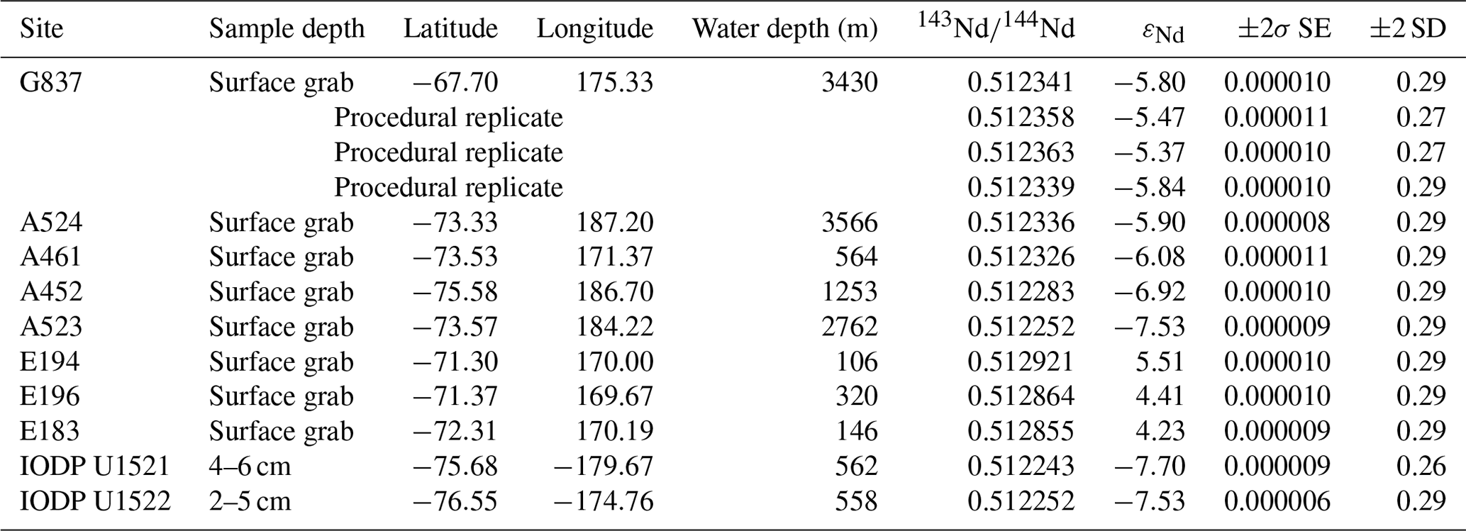
A uniform ε_Nd value of +5.3 was selected for Cenozoic volcanic rocks based on the consistent isotopic signature of such rocks throughout Marie Byrd Land and Victoria Land (Aviado et al., 2015; Martin et al., 2013; Phillips et al., 2018; Futa and LeMasurier, 1983; Hart et al., 1997). We emphasise, however, that the Kriging interpolation and 10 km spatial resolution used in our map implies that small areas of volcanic material will not result in such a high value. This was an intentional effect to partially account for the uncertainty in the presence of these subglacial volcanic rocks.

Adjacent to the Edward VII Peninsula, where outcropping rocks are sparse, the model consistently predicted ε_Nd values that were too radiogenic in comparison with seafloor surface sediment values which reach a mean of $-\mathrm{11.1}\pm \mathrm{0.4}$ (n=8) (Simões Pereira et al., 2018; Carlson et al., 2021). This was likely a result of an under-representation of the Swanson Formation on the Edward VII Peninsula in western Marie Byrd Land, as this rock group shows a close geochemical affinity with the glaciomarine shelf sediments in this area and may be widespread beneath the WAIS here (Simões Pereira et al., 2018). It was therefore assumed that the Swanson Formation, with an ε_Nd value of $\sim -\mathrm{12}$ (Korhonen et al., 2010; Yakymchuk et al., 2015), lies beneath most of the ice on the Edward VII Peninsula.

A5 Amundsen Sea and Bellingshausen Sea drainage sectors

Rock exposures around the Amundsen Sea embayment are particularly limited. Granites inferred to be present are assumed to be extensions of Mesozoic outcrops along this coast (Jordan et al., 2023). Cenozoic volcanics are extended, largely under Thwaites Glacier, using interpretations of magnetic, gravimetric and topographic data (Jordan et al., 2023) and airborne radar data that indicate enhanced subglacial melting due to elevated geothermal heat flux (Schroeder et al., 2014). Mafic rocks are assumed to include gabbros of Cenozoic age (Simões Pereira et al., 2020; Jordan et al., 2023), similar to Dorrell Rock near Mount Murphy (Rocchi et al., 2006). The bedrock surrounding these intrusions is assumed to be a mixture of typical West Antarctic rocks and assigned an ε_Nd value of −10 as described above.

A lack of rock outcrops and geophysical data translate to large uncertainties in the Bellingshausen Sea drainage sector of the WAIS (Fig. 5b). The Mesozoic granites and Antarctic Peninsula Volcanic Group present in the Antarctic Peninsula region, including the coastal region of the eastern Bellingshausen Sea, are extended based on continuation of magnetic anomalies, but there are no outcrops to confirm this assumption is correct. Values are predominantly set to −10, as described above for the WAIS interior, assuming a similar mixture of rock types is present. This matches with the ε_Nd values of sediments from beneath the floating terminus of Pine Island Glacier, which drains part of this region into the SE Amundsen Sea Embayment (Simões Pereira et al., 2020).

A6 Antarctic Peninsula

Rocks are relatively well exposed along the Antarctic Peninsula, with lithological extrapolation between outcrops possible using geophysical data (Golynsky et al., 2018) and geological mapping (Burton-Johnson and Riley, 2015). The ε_Nd values of many rock types are, however, relatively poorly constrained (see references in Simões Pereira et al., 2018, for available measured rock ε_Nd values). Fortunately, there is relatively little variation in Nd isotope compositions in this geologically young region, with ε_Nd values commonly ranging from $\sim -\mathrm{6}$ to −2, although some rocks have ε_Nd values clustered around $\sim -\mathrm{10}$ to −8 and $\sim +\mathrm{1}$ to +3 (Simões Pereira et al., 2018, and references therein). However, a relative lack of variation means uncertainty here is unlikely to substantially influence our results.

A7 Western Weddell Sea (West Antarctic side)

The extent of the Haag Nunatak block is taken from Jordan et al. (2020). It is possible this is overlain or intruded by rock types representing a continuation of Jurassic volcanic and magmatic activity recorded in rock outcrops on the Antarctic Peninsula. Furthermore, provenance data suggest that old (meta)sediments may be present on top of the Haag Nunatak block as the mean ε_Nd value of $\sim -\mathrm{7.4}$ for these rocks (Storey et al., 1994) is more radiogenic than that for seabed sediments recovered offshore from this part of the Ronne Ice Shelf (Williams et al., 2017).

Most rocks around the western Weddell Sea embayment are Cambrian–Permian sedimentary rocks, Cambrian volcanics or Mesozoic granites. Exposures are extended based on Jordan et al. (2013b), assuming outcrops are broadly representative of rocks present beneath the ice. The Cambrian volcanics and Mesozoic granites have been isotopically characterised, with respective mean ε_Nd values (±2 SD) of $-\mathrm{3.5}\pm \mathrm{4.3}$ (Curtis et al., 1999) and $-\mathrm{6.6}\pm \mathrm{3.4}$ (Pankhurst et al., 1991; Borg and DePaolo, 1994; Craddock et al., 2017), but no known ε_Nd measurements of the widespread Cambrian–Permian sedimentary strata have been performed. An ε_Nd value of −13 is assumed to be representative of these rocks based on temporal equivalents in the southern Transantarctic Mountains, such as the Byrd Group and non-volcanic beds of the Liv Group (Borg et al., 1990; Goodge et al., 2008; Marschalek et al., 2021). Neodymium isotope compositions of offshore sediments agree with this hypothesis (Williams et al., 2017). Beacon Supergroup and Ferrar Group outcrops in the Weddell Sea drainage sector follow the published mapping by Paxman et al. (2019) (see Sect. A1.3). The extent of the Dufek Intrusion (part of the Ferrar Group) is based on Ferris et al. (1998). Although we include the Weddell Sea drainage sector of the WAIS in our mapping, we do not include predictions for Weddell Sea offshore sediments in our results as these will also be influenced by supply of glaciogenic debris from East Antarctica, i.e. from sources that lie outside of our compilation area.

A8 New seafloor surface sediment data

To evaluate whether TASP produces accurate results, we compare the model predictions with seafloor surface sediment ε_Nd values. To improve the spatial coverage of these measurements, we include 10 new measurements from the Ross Sea (Table A2).

The methods used to generate these new data are identical to those described in Simões Pereira et al. (2018) and Marschalek et al. (2021). Briefly, the <63 µm fractions were leached to remove authigenic coatings, digested and subjected to standard ion exchange chromatography to isolate the Nd. The ${}^{\mathrm{143}}\mathrm{Nd}{/}^{\mathrm{144}}\mathrm{Nd}$ ratio was measured on a Nu instruments HR-ICP-MS in the MAGIC laboratories at Imperial College London. Measurements of BCR-2 processed alongside samples were consistently within the error of the published value (Weis et al., 2006), and blanks were 13 pg.