Climate model downscaling in central Asia: a dynamical and a neural network approach

High-resolution climate projections are essential for estimating future climate change impacts. Statistical and dynamical downscaling methods, or a hybrid of both, are commonly employed to generate input datasets for impact modelling. In this study, we employ COSMO-CLM (CCLM) version 6.0, a regional climate model, to explore the benefits of dynamically downscaling a general circulation model (GCM) from the Coupled Model Intercomparison Project Phase 6 (CMIP6), focusing on climate change projections for central Asia (CA). The CCLM, at 0.22° horizontal resolution, is driven by the MPI-ESM1-2-HR GCM (at 1° spatial resolution) for the historical period of 1985–2014 and the projection period of 2019–2100 under three Shared Socioeconomic Pathways (SSPs), namely the SSP1-2.6, SSP3-7.0, and SSP5-8.5 scenarios. Using the Climate Hazards Group InfraRed Precipitation with Station data (CHIRPS) gridded observation dataset as a reference, we evaluate the performance of CCLM driven by ERA-Interim reanalysis over the historical period. The added value of CCLM, compared to its driving GCM, is evident over mountainous areas in CA, which are at a higher risk of extreme precipitation events. The mean absolute error and bias of climatological precipitation (mm d⁻¹) are reduced by 5 mm d⁻¹ for summer and 3 mm d⁻¹ for annual values. For winter, there was no error reduction achieved. However, the frequency of extreme precipitation values improved in the CCLM simulations. Additionally, we employ CCLM to refine future climate projections. We present high-resolution maps of heavy precipitation changes based on CCLM and compare them with the CMIP6 GCM ensemble. Our analysis indicates an increase in the intensity and frequency of heavy precipitation events over CA areas already at risk of extreme climatic events by the end of the century. The number of days with precipitation exceeding 20 mm increases by more than 90 by the end of the century, compared to the historical reference period, under the SSP3-7.0 and SSP5-8.5 scenarios. The annual 99th percentile of total precipitation increases by more than 9 mm d⁻¹ over mountainous areas of central Asia by the end of the century, relative to the 1985–2014 reference period, under the SSP3-7.0 and SSP5-8.5 scenarios. Finally, we train a convolutional neural network (CNN) to map a GCM simulation to its dynamically downscaled CCLM counterpart. The CNN successfully emulates the GCM–CCLM model chain over large areas of CA but shows reduced skill when applied to a different GCM–CCLM model chain. The scientific community interested in downscaling CMIP6 models could use our downscaling data, and the CNN architecture offers an alternative to traditional dynamical and statistical methods.

1 Introduction

The increasing global mean temperature due to anthropogenic greenhouse gas emissions presents a significant challenge for society, requiring the assessment and prediction of future impacts on human health, natural ecosystems, and economies across different regions of the world (IPCC, 2021). Researchers conducting regional studies on the vulnerability, impacts, and adaptation typically achieve reliable high-resolution climate projections through dynamical downscaling via regional climate models (RCMs) (Rummukainen, 2010; Feser et al., 2011), statistical techniques (Maraun and Widmann, 2018; Fowler et al., 2007), or a hybrid of both approaches (Maraun et al., 2015; Meredith et al., 2018; Laflamme et al., 2016).

Central Asia (CA), recognised as one of the regions most vulnerable to climate change impacts, heavily depends on water resources from glaciers and rivers that are shrinking due to rising temperatures and decreasing precipitation (Reyer et al., 2017; Fallah et al., 2023; Didovets et al., 2024; Fallah and Rostami, 2024). The area faces significant challenges to food security characterised by declining crop yields and an increased occurrence of severe and frequent extreme weather events like floods and landslides. These conditions damage infrastructure, livelihoods, and agriculture, resulting in population displacement and migration (IPCC, 2021; Reyer et al., 2017).

Significant uncertainties inherent in the existing detailed observational and reanalysis datasets impede the development of high-resolution climate projections in CA (Fallah et al., 2016a). One option to complement these datasets is to use dynamical downscaling with RCMs. The Coupled Model Intercomparison Project Phase 6 (CMIP6) provides a framework for coordinated climate model experiments, enhancing our understanding of past, present, and future climate changes. Dynamical downscaling of CMIP6 models for the CA region is vital for accurately simulating extreme convective precipitation events which are influenced by the orography of the region (Lundquist et al., 2019; Ban et al., 2015; Wang et al., 2013; Frei et al., 2003; Russo et al., 2019), large-scale atmospheric circulation, and sea surface temperature anomalies in the Indian Ocean and the Pacific Ocean (Kendon et al., 2014; Demory et al., 2020; Xu et al., 2022). This method enhances the resolution of a driving general circulation model (GCM) and produces a physically consistent regional state of the climate. Despite some systematic biases, dynamical downscaling consistently provides high-quality datasets that accurately describe the climatology of all climate variables in CA (Qiu et al., 2022).

Various international institutions have collaborated within the Coordinated Regional Climate Downscaling Experiment (CORDEX) to address these issues and improve the inter-comparability of RCMs. CORDEX aims to create a robust framework for producing climate projections at a regional scale that is suitable for impact evaluation and adaptation planning globally. This effort aligns with the timeline of the Intergovernmental Panel on Climate Change's Sixth Assessment Report (Kikstra et al., 2022). However, most CORDEX research focuses on highly industrialised countries (IPCC, 2021; Taylor et al., 2012). Developing regions, including CA, bear the brunt of the consequences of global warming, yet they have access to only a limited number of CORDEX model simulations (Naddaf, 2022). As of the latest update, no simulation driven by CMIP6 has been planned for CORDEX CA (see https://wcrp-cordex.github.io/simulation-status/CMIP6_downscaling_plans.html, last access: 17 April 2024).

Beyond dynamical methods, recent developments in machine learning, including convolutional neural networks (CNNs), offer promising avenues for statistical downscaling (Harder et al., 2023; Rampal et al., 2024). CNNs have proven effective in numerous Earth science disciplines besides downscaling, such as classification (Gardoll and Boucher, 2022), segmentation (Galea et al., 2024), and prediction (Watson-Parris et al., 2022), thanks to their capacity to extract features from spatial data and identify nonlinear relationships between inputs and outputs. CNNs can recognise and encode spatial hierarchies in data (Zhu et al., 2017), making them exceptionally suitable for analysing geospatial data, a critical component in climate modelling. Unlike traditional statistical methods that often require manual selection and careful engineering of features, CNNs automatically learn the most predictive features directly from the data (Reichstein et al., 2019). They are generally more straightforward and efficient than traditional statistical downscaling methods for tasks aiming to predict or classify patterns distributed across spatial domains, such as temperature or precipitation patterns in climate models (Racah et al., 2017). CNNs are adept at maintaining spatial coherence in the output, which is critical in downscaling where preserving the geographical patterns of climate variables (like precipitation) is crucial (Kurth et al., 2018).

Researchers classify CNNs into two categories based on their last layer, namely (1) constrained and (2) unconstrained. Constrained CNNs integrate physical laws directly into the training process, such as mass, energy, or momentum conservation. This integration is achieved by modifying the loss function or the network's architecture to ensure compliance with these laws. In contrast, unconstrained CNNs do not explicitly incorporate physical laws or constraints. Instead, they rely solely on learning from the input data, generating output predictions based on the patterns detected in the data.

This study explores unconstrained and constrained CNN approaches to understand their effectiveness in downscaling and their performance when applied to GCMs not initially used for training.

The research questions guiding this study are as follows:

1. How effectively can CMIP6 models be downscaled to enhance precipitation simulations for the CORDEX central Asian region?

2. Can CNNs effectively downscale GCM outputs, and how do they perform when applied to GCMs that did not initially train them?

This article focuses on two main topics: (1) the added value of COSMO-CLM (CCLM) for representing precipitation over central Asia and (2) training a CCLM emulator using a CNN. We present data and methods in Sect. 2. Sections 3 and 4 introduce the results of dynamical and hybrid downscaling, respectively. Finally, we discuss the results and conclude in Sect. 5.

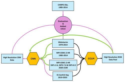
Figure 1 Schematic of the methodology used in this study. Green arrows show the data flow used for training the CNN, and magenta arrows are for the evaluation and calculation of the added values. Datasets are shown by rectangles, downscaling models by hexagons, and the evaluation analysis by a circle.

2 Data and methods

The methodology employed in this study is illustrated in Fig. 1.

2.1 Employed models and experimental setups

2.1.1 Regional climate model (RCM)

In this study, we conduct simulations using the CCLM regional climate model. Developed by the German Weather Service (DWD) and the German Climate Computing Center (Deutsches Klimarechenzentrum, DKRZ), CCLM originates from the COSMO numerical weather prediction model (Rockel and Geyer, 2008), which is widely utilised for short-term weather forecasting. Explicitly designed for regional climate simulation, CCLM enables researchers to investigate various aspects of the climate system, including temperature, precipitation, and extreme events. It has been extensively used to assess the impact of climate change across different regions such as Europe (Russo et al., 2022), Africa (Panitz et al., 2014; Dosio and Panitz, 2016), and Asia (Jacob et al., 2014; Kotlarski et al., 2014; Wang et al., 2013). Additionally, CCLM has been employed in climate projection studies to evaluate climate adaptation and mitigation strategies. The model has undergone thorough evaluation and validation (Fallah et al., 2016b; Russo et al., 2019; Kjellström et al., 2011), and its ability to generate realistic simulations of present climate conditions and variability has established it as one of the most widely used regional climate models in the scientific community (Sørland et al., 2021).

For our experiments, we utilised a model setup similar to the “optimal” configuration described by Russo et al. (2019). In their study, Russo et al. (2019) optimised the CCLM regional climate model for CA by adjusting the albedo based on forest fraction ratios and soil conductivity to account for the soil's liquid water and ice proportions. These modifications significantly improved the model's climatological performance and the distribution of incoming radiation, leading to more accurate climate representations for the region. According to the CORDEX protocol, simulations are divided into two primary phases. The first phase, the evaluation run, involves a single-model experiment over the period 1979–2014, using ERA-Interim reanalysis data at a spatial resolution of T255 (∼ 0.7°). The second phase, the projection run, utilises boundary conditions from GCMs of the CMIP6 project for the period 1950–2100 under various Shared Socioeconomic Pathways (SSPs). For this study, we selected the MPI-ESM1-2-HR GCM and considered the SSP1-2.6, SSP3-7.0, and SSP5-8.5 scenarios. SSPs represent baseline scenarios that describe future pathways based on population growth, technological advancement, economic development, urbanisation, and investments in healthcare, education, land use, and energy (Riahi et al., 2017).

Historical data for this study are based on greenhouse gas levels, land use, and other climate forcings observed from 1850 to 2014. The SSP scenarios used in the projections are as follows:

• SSP1-2.6 represents a “green” future, characterised by global efforts to protect resources, improve human well-being, and narrow income gaps. This scenario assumes low challenges to adaptation and low greenhouse gas emissions. Adaptation challenges in this context refer to the difficulties societies might face in adjusting to the impacts of climate change, including their susceptibility and the availability and the effectiveness of mitigation technologies and strategies. Under SSP1-2.6, global cooperation and sustainable practices lead to advancements in technology and governance, significantly reducing the vulnerability to climate change impacts. Societal structures are resilient, and resources are managed to minimise environmental stresses while maximising human well-being.

• SSP3-7.0 depicts a future characterised by regional rivalry, where nationalism and regional conflicts dominate, global issues are neglected, and inequality increases. This scenario involves a great number of challenges to adaptation and high greenhouse gas emissions.

• SSP5-8.5 represents a future of fossil-fuelled development with globally connected markets, rapid technological progress, and weak environmental policies. This scenario has fewer challenges to adaptation but results in very high greenhouse gas emissions.

For a comparison and evaluation of our RCM simulations, we have selected two CORDEX CA evaluation simulations from other models driven by ERA-Interim at a 0.22° horizontal resolution, namely (1) ERA-Interim-RMIB-UGent-ALARO-0 (Giot et al., 2016) and (2) ERA-Interim-GERICS-REMO2015 (Jacob and Podzun, 1997; Fotso-Nguemo et al., 2017).

2.1.2 CNNs

In this study, we develop a CNN-based emulator for the CCLM driven by the MPI-ESM1-2-HR GCM. This CNN utilises outputs from the GCM, covering the historical period from 1985 to 2014 and future scenarios spanning 2019 to 2100, as inputs to model the responses of the CCLM, which serves as the target. Given the low annual precipitation and significant spatiotemporal variability in many regions of CA, a comprehensive dataset that includes various precipitation patterns from both GCMs and RCMs is essential for effectively training the CNN to map from GCM to RCM outputs. To enhance model training, we have augmented our dataset with ERA-Interim reanalysis data and the corresponding CCLM simulations driven by it (ERA-Interim-CCLM) (see Fig. 1).

We train our CNN model based on the architecture proposed by Harder et al. (2023) (Fig. 2), which incorporates physical constraints to ensure mass conservation and energy balance. The model architecture features the following:

• Conv (convolutional layer). These layers help extract various levels of features from low-resolution images, such as edges, textures, and other relevant image details.

• ReLU (rectified linear activation unit). This nonlinear activation function introduces non-linearity and returns the input unchanged if it is positive; otherwise, it returns zero. This function enables the network to learn complex patterns efficiently.

• TransConv (transposed convolutional layer). This layer is crucial for downscaling. It increases the spatial dimensions of the feature maps, performing a sort of learnt interpolation. This allows the model to add details to the downscaled images based on the features extracted and processed in the earlier layers.

• ResBlock (residual block). These blocks allow the model to refine the initial lower-resolution predictions, which are downscaled (interpolated outputs) to a higher resolution. They enhance the model's ability to add fine details and textures (high-frequency information), improving the perceptual quality and sharpness of the images at an increased resolution.

In the context of deep learning for climate modelling, the “perfect model” approach involves starting with high-resolution data and intentionally upscaling it to a lower resolution. The machine-learning model is subsequently trained to reproduce the high-resolution data while receiving this artificial low-resolution input. The aim is to simulate a scenario in which the “truth” (the original high-resolution data) is known and then to recover this high resolution from the artificially upscaled data. This approach teaches the model the desired mapping from low to high resolution, enabling the model to effectively learn how to downscale or enhance the resolution, while minimising the loss of critical information. It is a controlled experiment that helps refine the model's capabilities.

The “imperfect model” approach, on the other hand, acknowledges that both the low-resolution (GCM output) and the high-resolution (RCM output) datasets have their inherent errors and limitations. In this scenario, we do not have a single source of truth but rather two separate sets of data, which are as follows:

• Low-resolution data. These data may capture global or large-scale phenomena but miss regional details (Xu et al., 2021; Chokkavarapu and Mandla, 2019).

• High-resolution data. These data provide detailed regional information but may still have errors or may not perfectly reflect reality due to limitations in data collection, model configuration, or computational constraints (Muttaqien et al., 2021).

In the imperfect model setup, the CNN's challenge is learning to map between two independently imperfect datasets. The CNN is trained to predict high-resolution details from low-resolution inputs as accurately as possible despite the absence of perfect ground truth. This process involves understanding and modelling the uncertainties and biases inherent in both datasets.

Prior to training, the dataset was randomly shuffled at the pair level to ensure that each GCM input and its corresponding RCM output remained together, preserving the intrinsic relationships between the coarse- and fine-resolution data. This approach prevents temporal or spatial autocorrelation from biasing the training process. It also improves the model's generalisation and performance by exposing it to various conditions. For the dataset distribution, 68 141 d (60 %) of RCM simulation data were used for training, 22 714 d (20 %) for validation, and 22 714 d (20 %) for independent testing. The low-resolution (GCM) dataset consists of 30×60 grid points, and the high-resolution (RCM) dataset comprises 120×240 grid points over latitudes and longitudes, respectively, resulting in a downscaling factor (N) of 4.

2.1.3 Constraint layers

We test the CNN with three different constraining methods in the last CNN layer (Harder et al., 2023), namely (1) hard constraining (HCL), (2) soft constraining (SCL), and (3) without constraining (NoCL). The setup of constraining is as follows: consider a factor N for downscaling in all linear directions, and let n:=N² and y_i, $i=\mathrm{1},\mathrm{\dots },n$ be the high-resolution patch values that correspond to the low-resolution pixel x. The mass conservation law has the following form:

$$\begin{array}{}\text{(1)}& {\displaystyle \frac{\mathrm{1}}{n}}\sum _{i=\mathrm{1}}^n{y}_i=x.\end{array}$$

Figure 2 Schematic of the CNN architecture for upsampling with the constraints layer two times. The inputs are low-resolution (LR) images sized 30×60, and the output is a super-resolution (SR) image sized 60×120. This figure is modified from Harder et al. (2023).

2.2 Validation and testing

According to Ciarlo` et al. (2021), the choice of observational data can significantly influence the perceived added value of an RCM, particularly when detecting extreme events, where poor-quality data might misleadingly suggest improved model performance. They recommend using observational datasets with spatiotemporal resolutions comparable to the model's for enhanced accuracy. In line with this, we use CHIRPS (Climate Hazards Group InfraRed Precipitation with Station data), a high-resolution gridded observational dataset, to validate the CCLM driven by the GCM. CHIRPS offers a resolution of 0.05°, covering latitudes from 50° N to 50° S, and provides independent observations derived from satellite and station data. This contrasts with reanalysis datasets which rely on climate model simulations (Funk et al., 2015).

For the validation of the CNN, however, we allocate 20 % of the CCLM simulation data as the target for evaluating the CNN emulator's performance rather than directly using CHIRPS. This is because the CNN is designed to emulate the climate output produced by the CCLM and not to match the observational data directly. While CHIRPS is used to validate the accuracy of the CCLM output, we validate the CNN by ensuring it accurately reproduces the CCLM's fine-scale climate information which has already been verified against CHIRPS for its realism.

We measure the added value of the CNN by comparing the MAE of the CNN outputs and the interpolated GCM outputs against the target CCLM output. This comparison assesses whether the CNN outperforms simple interpolation. The selected GCM and observational data are interpolated onto the RCM grid using the distance-weighted average method. Ciarlo` et al. (2021) noted that such an interpolation might create unrealistic values as it does not account for the physical processes and could introduce artefacts, depending on the interpolation method, the spatial distribution of data points, and the resolution ratio. Therefore, we use simple interpolation as a baseline, recognising its limitations in preserving the statistical properties of precipitation, which does not follow a normal distribution. Following (Hodson, 2022), we apply the MAE as an evaluation metric to quantify the biases in emulated and dynamically downscaled precipitation (y_t) against observations (O) as follows:

$$\begin{array}{}\text{(5)}& \text{MAE}={\displaystyle \frac{\mathrm{1}}{T}}\sum _{t=\mathrm{1}}^T|y_t-O_t|,\end{array}$$

where T represents the number of time steps over 30 years of daily data.

We define the added value (AV) as the reduction in MAE achieved by the downscaling relative to the driving GCM as follows:

$$\begin{array}{}\text{(6)}& \text{AV}={\text{MAE}}_{\mathrm{GCM}}-{\text{MAE}}_{\mathrm{CCLM}},\end{array}$$

where MAE_GCM and MAE_CCLM are the differences between interpolated GCM and RCM with respect to the reference CHIRPS dataset.

As an additional metric, we also use the climatological bias; i.e. the difference between the model and observations is as follows:

$$\begin{array}{}\text{(7)}& \text{BIAS}={\text{PR}}_y-{\text{PR}}_{\mathrm{O}}.\end{array}$$

Figure 3 (a) CCLM simulation domain over central Asia and the topography (m). (b) CHIRPS climatology for 1985–2014 (average of daily values over all years in mm d⁻¹). (c) WorldClim weather stations (red dots).

3 Results

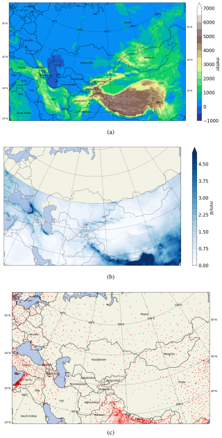
Figure 3a illustrates the topography of the CORDEX CA simulation domain. Figure 3b displays the mean daily precipitation averaged over the years 1985–2014 (mm d⁻¹) and derived from CHIRPS data. The regions with the highest precipitation are the mountainous areas of CA, particularly notable in the Asian summer monsoon region north of India and along the Himalayas in the southeastern part of the domain, where precipitation values are pronounced. Figure 3c depicts the distribution of WorldClim weather stations (Fick and Hijmans, 2017) across CA, serving as a proxy for the density of station data used in the CHIRPS dataset. Observational data are sparsely distributed in East China, especially over the Tibetan Plateau. Consequently, data–model comparisons are considered unreliable in this region (Randall et al., 2007; Cui et al., 2021; Yan et al., 2020; Russo et al., 2019).

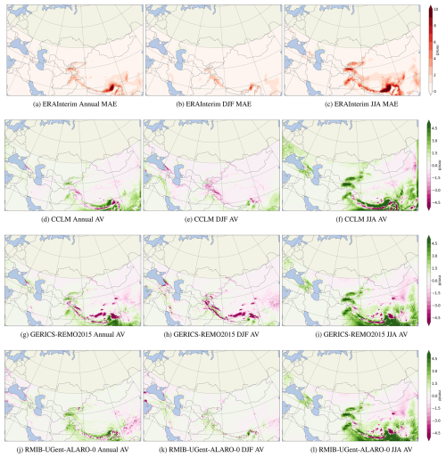
Figure 4 Mean absolute error (MAE) of daily precipitation (mm d⁻¹) from ERA-Interim, as well as the added value (AV), as measured by MAE differences between ERA-Interim and RCMs (MAE_ERA-Interim−MAE_RCM) (in mm d⁻¹) for annual amounts (a, d, j, i), amounts in December, January, and February (b, e, h, k) and amounts in June, July, and August (c, f, i, l). CHIRPS is used as the observation. All datasets are interpolated to the CCLM grid.

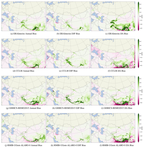
Figure 5 Bias of climatological precipitation (mm d⁻¹) from ERA-Interim, as well as the ERA-Interim-driven RCMs (PR_{ERA-Interim-CCLM}−PR_OBS) (in mm d⁻¹) for annual amounts (a, d, j, i), amounts in December, January, and February (b, e, h, k) and amounts in June, July, and August (c, f, i, l). CHIRPS is used as the observation.

3.1 Added value of CCLM driven by ERA-Interim

To characterise the overall performance of the CCLM model across time and space, Figs. 4 and 5 present maps displaying annual, winter (December, January, and February – DJF), and summer (June, July, and August – JJA) MAE and mean biases. These biases in precipitation are calculated between the interpolated ERA-Interim data and CCLM outputs driven by ERA-Interim for the period 1985–2014 in comparison to CHIRPS (see Eqs. 5 and 6). Figure 4a–c illustrate the MAE for ERA-Interim for annual, winter, and summer averages. The added value of the CCLM RCM compared to the interpolated ERA-Interim is depicted in Fig. 4d–f. During the Asian summer monsoon, the CCLM MAE is high (5 mm d⁻¹) with respect to the GCM over the south and southeast of the domain (regions in magenta), whereas it is generally lower (<1 mm d⁻¹) during winter. In the mountainous areas of Afghanistan, Kyrgyzstan, and Tajikistan, CCLM is closer to observations than GCM. However, the GCM is closer to observations near the domain's southern boundaries for annual values and in the south and southeast during summer.

The AVs of GERICS-REMO2015 and RMIB-UGent-ALARO-0 driven by ERA-Interim are presented in Fig. 4g–l, using CHIRPS as the observational dataset. The added value of the RCM is most pronounced in areas with complex topography, especially during summer, across all three RCMs (Fig. 4f, i, and l). Areas where the RCM has a smaller MAE than the reanalysis in comparison to observations are found over Tajikistan, Kyrgyzstan, northern Afghanistan, and part of the Himalayas – regions that are crucial water sources for post-Soviet states. The annual AV patterns still show positive values in these regions (Fig. 4d, g, and j). GERICS-REMO2015 has less skill than the reanalysis during winter and for annual values over large portions of mountainous areas.

For annual values, all three RCMs reduce the large- and local-scale bias of ERA-Interim, especially in regions with complex topographies. However, the nested RCMs exhibit similar MAE values near their lateral boundaries, relative to their driving model (Fig. 4a–c). This is likely due to the RCM being constrained by the boundary conditions imposed by the GCM, limiting the RCM's ability to generate its own internal variability. As a result, negative AV quantities may arise from boundary effects, particularly near the eastern and southeastern edges, where the model is less free to improve upon the monsoonal precipitation patterns set by the driving GCM. This is also reflected in the model climatology biases in Fig. 5. These biases are particularly evident in the lower-right corner of the domain during JJA and across the Tibetan Plateau throughout the year, likely influenced by the constraints imposed by the GCM's boundary conditions. In these regions, the errors in the RCM closely mirror those of the GCM, suggesting that the RCM is heavily constrained by the lateral boundary conditions. Moreover, across other parts of the domain, the RCM tends to inherit the biases of the GCM for 30-year climatological means as large-scale errors in the driving GCM propagate through the nested model. However, despite these limitations, RCMs are more capable of capturing extreme weather events, such as heavy precipitation (see Fig. A1), which are often underrepresented in GCMs due to their coarse resolution (Rai et al., 2024).

3.2 Extreme precipitation patterns in CCLM and CMIP6 GCMs

Given that the CCLM simulation has demonstrated added value for precipitation over the mountainous regions of CA, we explore climate change signals in its high-resolution output. These high-resolution maps may inherit biases from the GCM–RCM selection and could vary under different anthropogenic forcings. We assume that many model biases are consistent across different time slices and, therefore, can be removed when calculating changes between the historical period (1985–2014) and future periods (2070–2099).

We present climate change trends in CCLM and the CMIP6 GCMs ensemble statistics (ensemble mean and standard deviation). We analysed 31, 33, and 38 models for SSP1-2.6, SSP3-7.0, and SSP5-8.5 scenarios, respectively, with a total of 158, 185, and 242 simulations (see the Supplement for the list of models used). We calculate statistics over each model's members to ensure equal weighting for individual models before building the final statistics. We have selected the yearly 99th percentile of daily precipitation (PR99), which accounts for the 3 d with the highest precipitation each year. Additionally, we chose the number of very heavy precipitation days during the period (ECA–RX20mm) as another index, which is commonly used in climate research to assess the impacts of heavy precipitation events on water resources, agriculture, and natural ecosystems (Klok and Klein Tank, 2008).

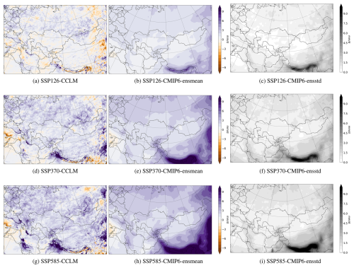
Figure 6 Changes in the averaged yearly 99th percentile (3 d per year) of total precipitation (mm d⁻¹) with respect to 1985–2014 references for (a, b) SSP1-2.6, (d, e) SSP3-7.0, and (g, h) SSP5-8.5 at the end of the century (2070–2099) from the CCLM and CMIP6 GCM ensemble means. The ensemble's standard deviations are shown in panels (c), (f), and (i).

Figure 6 shows the changes in PR99 at the end of the century (2070–2099) compared to the historical period (1985–2014) for CCLM (Fig. 6a, d, g) and CMIP6 GCMs (Fig. 6b, e, h) under different scenarios. The large-scale patterns remain consistent across all three scenarios, intensifying with increased anthropogenic influence. The standard deviation of the models' ensemble is depicted in Fig. 6c, f, and i. Our analysis indicates that the Himalayas, particularly Nepal, north India, and Bhutan, exhibit the highest uncertainty among the GCMs in all scenarios. Except for this region and the eastern boundary of the domain, the standard deviation remains below 3 mm d⁻¹. Under the SSP5-8.5 and SSP3-7.0 scenarios, regions including northwest India, north Pakistan, north and southwest Iran, and the south and southeast of the Black Sea are projected to experience increases in PR99 values exceeding 9 mm d⁻¹. A reduction in PR99 is detected in the eastern Mediterranean, specifically in Jordan, Syria, and southern Türkiye. Similar patterns are observed in the CMIP6 ensemble mean, but due to averaging, the ensemble mean patterns are approximately ±5 mm d⁻¹ over these areas. Under the SSP1-2.6 scenario, which is aligned with the 2 °C warming target, the previously observed increases in precipitation exceeding ±9 mm d⁻¹ for CCLM and ±5 mm d⁻¹ for GCMs are no longer evident. In CA, areas such as Kyrgyzstan, Tajikistan, northern Pakistan, and southwestern Iran are particularly vulnerable to rainfall-induced hazards, including landslides (Wang et al., 2021; Kirschbaum et al., 2010) and floods (e.g. the Pakistan floods of 2010 and 2022).

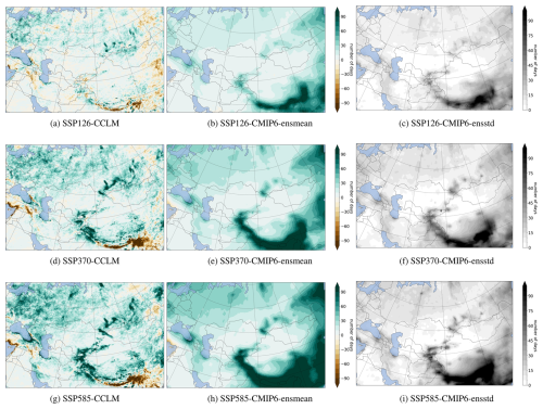
Figure 7 Changes in number of days with precipitation of more than 20 mm in the period with respect to 1985–2014 references for (a, b) SSP1-2.6, (d, e) SSP3-7.0 and (g, h) SSP5-8.5 at the end of the century (2070–2099) from the CCLM and CMIP6 GCM ensemble mean. The ensemble's standard deviations are shown in panels (c), (f), and (i).

Figure 7a, d, and g illustrate the changes in ECA–RX20mm values for CCLM at the end of the century across three scenarios with respect to the historical period of 1985–2014. The observed patterns align with those in Fig. 6, underscoring an increase in the frequency of very heavy precipitation days, particularly marked over the Tibetan Plateau, as anthropogenic influences intensify. Similarly, Fig. 7b, e, and h reveal that the CMIP6 GCM ensemble mirrors the behaviour observed in CCLM. However, the ensemble standard deviations for ECA–RX20mm values rise over Tajikistan and Kyrgyzstan, as shown in Fig. 7c, f, and i. The growing frequency and intensity of extreme precipitation events over the elevated regions of central Asia, driven by anthropogenic factors, are a cause for concern (Fallah et al., 2023). This CCLM simulation enhances our understanding of how the dynamical downscaling sensitivity to different levels of anthropogenic forcing can vary locally.

4 CCLM emulator using a CNN

In this study, we create a CCLM emulator for precipitation over CA. We aim to establish that this emulator outperforms a simple interpolation, particularly in areas experiencing extreme precipitation. We aim to show that the CCLM emulator can replicate CCLM-like precipitation patterns when driven by the parent GCM.

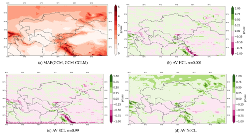
Figure 8 Performance based on shuffled testing data (22 714 d or 20 % of the dataset). (a) Mean absolute error (MAE) between the GCM(MPI-ESM1-2-HR) and the RCM (CCLM). MPI-ESM1-2-HR is remapped bilinearly to the 0.25×0.25 grid. (b–d) Added value (AV) or MAE(MPI-ESM1-2-HR,CCLM) − MAE(CNN,CCLM) for different constraining methods.

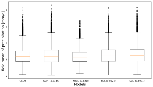
Figure 9 Boxplot of averaged daily precipitation over the central Asian domain (shown in Fig. 7) for different models and test datasets (22 714 d or 62.2 years). Numbers in the parentheses indicate the correlation coefficients between each model and the CCLM simulation.

Focusing on the CA domain, which encompasses post-Soviet states (Kazakhstan, Kyrgyzstan, Tajikistan, Turkmenistan, and Uzbekistan), we exclude the broader CORDEX CA domain shown in Fig. 3. This domain is the region of interest in the Green Central Asia project https://www.greencentralasia.org/en (last access: 13 January 2025), which the German Foreign Office finances. Figure 8a illustrates the MAE of the interpolated MPI-ESM1-2-HR, using the CCLM output as the “true” precipitation. CCLM generates distinct precipitation patterns, particularly in areas with complex topography. Assuming CCLM as the ground truth, we examine whether the CNN can replicate these outputs using the GCM as input. To assess the emulator's effectiveness, we present added value maps (relative to the reference RCM) in Fig. 8b–d. A comparison of MAE reduction maps reveals that the unconstrained CNN demonstrates significant skill over elevated regions of CA, whereas constrained runs show less noticeable pattern changes. For instance, the HCL and SCL emulators generate closely mixed negative and positive added values across elevated areas, while NoCL consistently exhibits positive values across the domain. Several artefacts in the MAE reduction maps of constrained models, particularly over northern India, reflect the shape of the GCM grid. We also produce boxplots of daily precipitation for the CA domain to explore the distribution improvements (Fig. 9). Correlation coefficients between the time series averages of precipitation across the domain and CCLM are presented in Fig. 9 (values in parentheses). Among the daily averages, NoCL achieves the best performance (highest correlation coefficient of 0.8318), although it records fewer outliers than CCLM and other model simulations. The distribution is concentrated around the median, exhibiting the narrowest interquartile range. The distribution profiles of both constrained models (HCL and SCL) resemble those of the interpolated GCM, which is expected since the constraints maintain mass consistency within corresponding grid boxes (Eq. 1).

Applying the CNN to a different GCM

We evaluate the emulator's generalisation ability, i.e. its capacity to generate reliable predictions on new datasets. We chose NoCL for its superior performance among the three CNNs. We conduct a new 15-year dynamical simulation using CCLM, driven by the EC-Earth3-Veg (Döscher et al., 2022) GCM under the SSP3-7.0 scenario from 2019 to 2033. These data serve as input to our CCLM emulator, which was previously trained to emulate CCLM outputs using MPI-ESMI-2-HR. Although EC-Earth3-Veg may appear distinct from MPI-ESM1-2-HR, it shares the same forcing information tied to the SSP3-7.0 scenario. This could lead to similar climate outputs despite their differences. Therefore, the two datasets used for training and prediction might not be as distinct as they seem, possibly contributing to the emulator's generalisation performance.

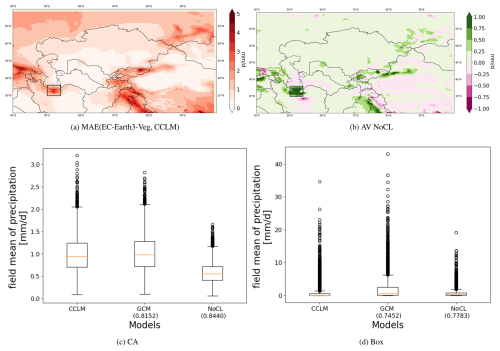
Figure 10 (a) Mean absolute error (MAE) between the GCM(EC-Earth3-Veg) and the RCM (CCLM). The GCM is remapped bilinearly to the 0.25×0.25 grid. (b) The added value (AV) or MAE reduction (MAE(EC-Earth3-Veg,CCLM) − MAE(CNN,CCLM) for unconstrained method. Panels (c) and (d) show boxplots of averaged daily precipitation over the CA domain and the black box shown in panels (a) and (b) over the north of Iran. Numbers in the parentheses indicate the correlation coefficients of each model with respect to CCLM.

The trained NoCL model was applied to the unshuffled EC-EARTH3-Veg data for new predictions. Figure 10a presents the MAE of the interpolated EC-Earth3-Veg with respect to the dynamical downscaling with CCLM. The MAE pattern of EC-Earth3-Veg closely mirrors that of MPI-ESM1-2-HR (Fig. 8a). The NoCL emulator does not consistently show positive AV across the domain (Fig. 10b) as was previously observed when applied to the MPI-ESM1-2-HR. The emulator learnt relationships between MPI-ESM1-2-HR and CCLM, which may be specific to these models and might not necessarily apply to the new EC-Earth3-Veg and CCLM configuration. As demonstrated previously, the RCM state depends on the state of its driving GCM. CCLM is driven at the lateral boundaries by the GCM values for state variables (temperature, pressure, wind speed, etc.) and not by precipitation, which is the input of the CNN. The precipitation inputs from the two GCMs carry different biases, complicating the transfer of mapping from MPI-ESM1-2-HR-driven CCLM outputs to those driven by EC-Earth3-Veg.

Despite these challenges, the CNN model demonstrates added values exceeding 1 mm d⁻¹ in regions such as the Alborz mountains and the southern Caspian Sea in northern Iran (highlighted in black rectangles in Fig. 10a and b) and parts of Tajikistan and Kyrgyzstan. An exploration of the daily precipitation distribution field mean indicates that the CNN's median value and outliers are lower than those of the EC-Earth3-Veg and CCLM simulations (Fig. 10c). The day-to-day correlation has improved in NoCL with respect to GCM, increasing the correlation coefficient from 0.815 (EC-Earth3-Veg) to 0.844 (NoCL). Over the highlighted area in Fig. 10b, where the NoCL model has a lower MAE than the GCM, the distribution of precipitation resembles that of CCLM, encompassing the region with the highest rainfall in Iran, which is vital for a large portion of the population, including Tehran. Only the outliers larger than 20 mm d⁻¹ are not reconstructed by NoCL.

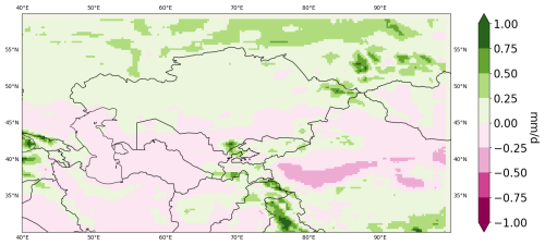
Figure 11 The added value (AV) or MAE reduction (MAE(EC-MPI-ESM1-2HR, CCLM) − MAE(CNN, CCLM)) for an unconstrained method that was not trained but applied to the SSP3-7.0 scenario.

As a further test of generalisation, we intentionally excluded the SSP3.7-0 scenario from the training process. This allowed us to apply the model to a specific simulation and assess its ability to handle an unknown type of forcing. Figure 11 demonstrates the AV of the CNN emulator for SSP3-7.0 in comparison to the dynamical downscaling with CCLM, revealing that the AV pattern is strikingly similar to that shown in Fig. 8d. This confirms that the CNN shows promise for learning and reproducing the patterns under different forcing scenarios it was not explicitly trained on, as demonstrated by its performance with the SSP3.7-0 scenario.

5 Discussion and conclusions

Regional climate change impact assessments require high-resolution climate projections. The main strategies to produce such datasets are statistical and dynamical downscaling, as well as a hybrid of the two methods. Statistical downscaling often struggles to account for the dynamic influences of complex landscapes, including topography and varying surface parameters such as vegetation, soil types, and waterbodies like lakes, which may affect the accuracy of statistical relationships (Li et al., 2022). For statistical downscaling methods applied to precipitation, observations need to contain detailed information about precipitation distribution in areas with complex topography (Lundquist et al., 2019).

Conversely, dynamical downscaling requires massive computational time and data storage. For example, a 30-year CCLM simulation driven by ERA-Interim took roughly 1 week to complete using 216 processors of the HLRE-4 Levante computer at the German Climate Computing Center (DKRZ). Additionally, the added value of RCMs is still debated as they are highly dependent on the driving GCMs.

In this study, we contributed to the dynamic downscaling efforts over the CORDEX CA domain, taking a small step towards creating an RCM ensemble for CA. A single RCM simulation helps identify model biases and uncertainties that need to be addressed in future model improvements. It is essential to note that a single-model run for CMIP6, instead of an RCM ensemble, may not provide a comprehensive understanding of potential climate change impacts on a region. Therefore, it is recommended that researchers conduct multiple simulations with different initial and boundary conditions and model configurations to account for the uncertainty associated with climate projections.

In the first part of the study, we demonstrated the added value of RCMs (using the CCLM model) over GCMs for CA in representing precipitation. Our CCLM run showed added value with respect to its driving GCM, comparable to the range of values obtained for other RCMs applied to the CORDEX CA domain over the evaluation period. It also reproduced extreme precipitation patterns similar to the CMIP6 ensemble mean projections for the end of the century. The CCLM and CMIP6 ensembles indicated an increased risk (in terms of intensity and frequency) of heavy precipitation events in vulnerable regions of CA due to various human activities.

Our study evaluated the downscaling skill of RCM using high-resolution observations, a crucial step for accurately capturing localised climate phenomena. This evaluation was essential before further study steps and regional adaptation strategies could be implemented. In future work, it would be valuable to follow the approach suggested by Volosciuk et al. (2017), where downscaling outputs are evaluated at coarser resolutions. This would allow for a deeper understanding of how downscaling methods introduce or fail to correct biases, which can vary significantly across spatial scales. By conducting evaluations on a coarser grid, we can better distinguish between the inherent biases of the model and those introduced by the downscaling process, providing important insights into the limitations and strengths of downscaling techniques in representing climatic variables across different scales.

We showed that a single GCM–RCM model chain could be used to train a climate emulator based on a CNN model. It learnt relationships between the coarse- and fine-resolution datasets, addressing the issue of spatial intermittency – where data points are unevenly distributed or missing across space – common in some statistical downscaling approaches (Harder et al., 2023). However, we also demonstrated that the CNN model had limitations when generalising, as it did not achieve a robust error reduction pattern when given a different GCM as input. The learning process strongly depended on the GCM–CCLM relationships. More importantly, an RCM is usually forced to follow its driving GCM and can only produce extra information on a local scale. The presented CNN could be applied to other experiments of the same GCM.

We deliberately excluded the SSP3-7.0 scenario from the training dataset to evaluate the model's generalisation capabilities for other scenarios of the same GCM. This strategy allowed us to assess whether the model could effectively infer and replicate patterns from untrained scenarios. The model's output for the SSP3-7.0 scenario exhibited an AV pattern that mirrored the dynamical downscaling results of the CCLM driven by the same SSP3-7.0 scenario. This alignment supported the notion that our CNN emulator could learn from its training data and generalise to new and unseen conditions.

This work was an initial step in demonstrating the potential of such a hybrid approach. We encourage the community to explore different model structures and parameter combinations for further improvement. For example, our initial setups showed that a physically constrained CNN setup that applies a linear transformation to ensure mass or energy conservation between the low- and high-resolution images did not successfully downscale precipitation. The original dataset might not satisfy the constraints, leading to suboptimal results. In contrast, with a higher degree of freedom, the unconstrained CNN produced patterns closer to the target RCM. Future studies could test alternative machine learning models, such as generative adversarial networks (GANs), which can generate more high-frequency patterns and improve the downscaled output. Additionally, incorporating more information into the CNN by adding characteristics like surface height, vegetation, land cover, and land use as new channels within the input layer could enhance model performance.

Appendix A: Precipitation distribution

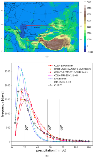
Figure A1 (a) Free zone within the study region over central Asia. The dashed box (110×76 grids) is selected as the free zone for further data–model comparisons. (b) Precipitation distribution of maximum daily values in the free zone shown from different RCMs, GCMs, and CHIRPS for the period 1985–2014. Vertical lines show different percentiles of the CHIRPS dataset on the x axis.

To further explore the added value of dynamical downscaling in the estimation of precipitation distribution, we calculated the histogram of daily precipitation (for grid points where precipitation >1 mm d⁻¹) for the daily maximum value in the free zone (the red box shown in Fig. A1a). We select a free zone such that it is far from the lateral boundaries and located within the CHIRPS data coverage (south of 50° N). Therefore, we assume that the RCMs can freely create their climate state (internal climate variability) within this box and that the influence of the GCM boundary conditions is minor. As expected, ERA-Interim and MPI-ESM1-2-HR have shorter right tails and a higher maximum frequency than the CHIRPS dataset (Fig. A1b). They do not show many values greater than 70 mm d⁻¹. Increasing the resolution via the dynamical downscaling, all the RCMs create extreme values, as seen in the observation, and have longer right tails. Both CCLM simulations show a similar distribution, and their maximum frequencies are closer to the one from CHIRPS than the other two RCMs. This agrees with the findings of Ciarlo` et al. (2021), who showed that the added value is more considerable for higher-precipitation percentiles. We know that such a comparison between the GCM and RCM probability is not “fair”. Comparisons are usually conducted at the coarser resolution, and RCM values must be aggregated to GCM grids. However, we are interested in the added value of different RCMs, especially for the extreme values and aggregation to the coarser grid will degrade the spatial statistics of the local higher-resolution phenomena. It has been previously shown that RCMs have higher skills when simulating extreme precipitation events than GCMs (Gao et al., 2015; Rajczak et al., 2013; Feser et al., 2011).

Appendix B: CNN runs

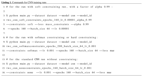
We used the following commands for training the CNN model based on Harder et al. (2023).

Note that the datasets and codes are available via Zenodo (https://zenodo.org/records/10417111, Fallah, 2023), with comprehensive details utilised in the paper.

Listing B1 Commands for CNN training runs.