Empirical modeling of tropospheric delays with uncertainty

Accurate modeling of tropospheric delay is important for high-precision data analysis of space geodetic techniques, such as the Global Navigation Satellite System (GNSS). Empirical tropospheric delay models provide zenith delays with an accuracy of 3 to 4 cm globally and do not rely on external meteorological input. They are thus important for providing a priori delays and serving as constraint information to improve the convergence of real-time GNSS positioning, and in the latter case proper weighting is critical. Currently, empirical tropospheric delay models only provide delay values but not the uncertainty of delays. For the first time, we present a global empirical tropospheric delay model, which provides both the zenith delay and the corresponding uncertainty, based on 10 years of tropospheric delays from numerical weather models (NWMs). The model is based on a global grid and, at each grid point, a set of parameters that describes the delay and uncertainty in the constant, annual, and semiannual terms. The empirically modeled zenith delay has agreements of 36 and 38 mm compared to 3-year delay values from the NWM and 4-year estimates from GNSS stations, which is comparable to previous models such as Global Pressure and Temperature 3 (GPT3). The modeled zenith tropospheric delay (ZTD) uncertainty shows a correlation of 96 % with the accuracy of the empirical ZTD model over 380 GNSS stations over the 4 years. For GNSS stations where the uncertainty annual amplitude is larger than 20 mm, the temporal correlation between the formal error and smoothed accuracy reaches 85 %. Using GPS observations from ∼ 200 globally distributed IGS stations processed in kinematic precise point positioning (PPP) mode over 4 months in 2020, we demonstrate that using proper constraints can improve the convergence speed. The formal error modeling is based on a similar dataset to that of the GPT series, and thus it is also applicable for these empirical models.

1 Introduction

For space geodetic techniques such as the Global Navigation Satellite System (GNSS), very-long baseline interferometry (VLBI), and satellite altimetry, microwave signals transmitting through the troposphere are delayed and bent due to the non-vacuum conditions of the troposphere, causing the tropospheric delay. The total tropospheric delay could be divided into hydrostatic and wet parts. The former accounts for 90 % of the total delay and is strongly dependent on the atmospheric pressure, and at sea level height this is around 2 m in the zenith direction. The latter is closely related to the water vapor and can hardly be modeled due to the unpredictability of water vapor in space and time. In data processing of these space geodetic techniques, the tropospheric delay is usually modeled as the zenith delay (zenith hydrostatic delay ZHD and zenith wet delay ZWD) and the mapping functions, and in high-precision applications horizontal gradients should also be considered (Böhm and Schuh, 2013).

Tropospheric zenith delay can be derived using several approaches, including in situ meteorological observations combined with models such as the Saastamoinen or Hopfield functions (Askne and Nordius, 1987; Hopfield, 1969; Saastamoinen, 1972); radiosonde measurements, which provide vertical profiles of meteorological data (Chen and Liu, 2016; Liou et al., 2001; Wu et al., 2019); and water vapor radiometers, which directly measure atmospheric water vapor content (Braun et al., 2003; Niell et al., 2001). Additionally, numerical weather models (NWMs) offer tropospheric delays on a global scale by integrating meteorological data vertically (Böhm et al., 2007; Kouba, 2007; Landskron and Böhm, 2017). Although these approaches can yield high accuracy, typically within 5 mm to 2 cm, they all require access to accurate meteorological information, which may not be available to real-time GNSS users. Another option is the empirical tropospheric delay model, which aims to represent the tropospheric delay with a set of simplified parameters. The empirical tropospheric delay model usually only requires a user's location (latitude, longitude, and height) and time as input. Therefore, it has the advantage of being free of external data communication and easy to compute. However, the empirical models usually have an accuracy of 3 to 5 cm with respect to NWM or GNSS estimates, depending on the resolution of the model and, more importantly, the water vapor content of the location (Böhm et al., 2015; Ding and Chen, 2020; Kos et al., 2009; Li et al., 2014; Penna et al., 2001; Yao et al., 2016, 2015).

The empirical tropospheric delay models are usually based on radiosonde observations (Leandro et al., 2007) or NWM-derived products (Böhm et al., 2015; Lagler et al., 2013; Landskron and Böhm, 2017; Li et al., 2012; Yao et al., 2015), and the zenith hydrostatic and wet delays are provided by global grids, spherical harmonic functions, or lookup tables. In the Global Pressure and Temperature (GPT) models (Böhm et al., 2015; Kouba, 2009; Lagler et al., 2013; Landskron and Böhm, 2017), atmospheric pressure, temperature, and water vapor are provided given the location and time, and thus the zenith delays can be calculated using the Saastamoinen (1972) and Asknew and Nordius (1987) equations. Unlike the GPT series, which are based on European Centre for Medium-Range Weather Forecasts (ECMWF) products, the TropGrid2 model is based on the National Center for Environmental Prediction (NCEP) product and directly provides ZHD and ZWD instead of the meteorological parameters (Schüler, 2013). Similarly, the IGGtrop models are also based on the NCEP products and directly provide zenith delays (Li et al., 2014, 2018, 2012). The global zenith tropospheric delay (GZTD) models are based on the ECMWF-derived Vienna mapping function (VMF) products and provide zenith delay using a spherical harmonic function (Yao et al., 2016). The Improved Tropospheric Grid (ITG) model provides tropospheric delays and additional meteorological data (Yao et al., 2015). Slight improvements are reported with refined modeling methods, e.g., including the diurnal periodical terms, adopting more complicated functions in modeling the altitude scaling, and increasing the spatial resolution (Hu and Yao, 2018; Huang et al., 2021, 2022; Mao et al., 2021; Sun et al., 2019; Wang et al., 2022a; Xu et al., 2020; Zhou et al., 2022; Zhu et al., 2022). Chen et al. (2020) presented an empirical ZTD model over mainland China based on the GNSS ZTD estimates, and Li et al. (2021) combined radiosonde observations with NWM products to determine empirical meteorological models. The agreement of these empirical models with other sources, e.g., GNSS estimates or radiosonde observations, varies between 3 and 5 cm.

Due to the correlation between receiver clocks, tropospheric parameters, and station coordinates, using accurate external tropospheric delay products with proper weighting can improve the convergence of precise point positioning (PPP), especially in real-time applications where fast convergence is of great interest. The NWM-derived ZTD usually agrees with GNSS at the level of 1 to 1.5 cm, and regional tropospheric delay modeling can reach an accuracy of better than 1 cm. They are therefore used to enhance the real-time PPP convergence time (Cui et al., 2022; de Oliveira et al., 2016; Douša et al., 2018; Lu et al., 2017; Takeichi et al., 2009; Wilgan et al., 2017; Zhang et al., 2017; Zheng et al., 2017). In situ instruments such as a water vapor radiometer and Raman lidar could provide high-precision tropospheric delays (within 1 cm) and are also investigated to improve precise GNSS data processing (Alber et al., 1997; Bock et al., 2001; Bosser et al., 2009; Wang and Liu, 2019; Ware et al., 1993). It is also demonstrated that empirical tropospheric delay models can improve the convergence of GNSS PPP (Chen et al., 2020; Yao et al., 2017, 2014). Due to the different accuracies of these external tropospheric delay products, it is necessary to properly weight them when constrained in GNSS analysis. An overly tight constraint would introduce errors and degrade the accuracy of the estimates, whereas an overly loose constraint can hardly contribute to reducing the convergence time. When using the NWM-derived or regionally modeled tropospheric delays, the weighting strategy is usually based on either the statistic of a large number of stations or numerically tested criteria.

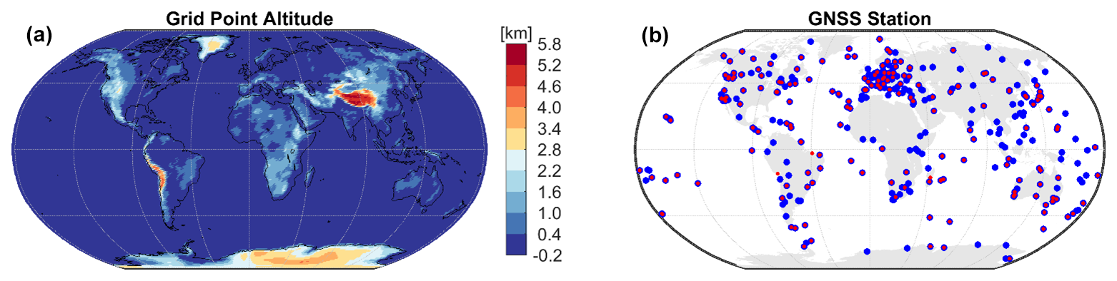
Figure 1 Altitude (ellipsoidal height) of the VMF3 grid points (a) and the distribution of the GNSS stations (b). The GNSS stations used for the ZTD comparison and PPP validation are given by the blue and red dots, respectively.

Currently, most empirical tropospheric delay models only provide the delay values but not the uncertainty for these delays. Chen et al. (2020) proposed a regional empirical ZTD model based on GNSS ZTD estimates in the mainland China region, where formal errors are also provided. Motivated by using empirical tropospheric delay models to enhance real-time GNSS positioning, in this work we aim to provide both tropospheric delays and the corresponding uncertainties on a global scale. We first fit the ZTD time series using the commonly adopted functions, i.e., the constant plus annual and semiannual periodical terms. The VMF ZTD global grids with a temporal resolution of 1° × 1° in the period 2009–2018 are used. After obtaining the fitting residuals at each grid point, we further model the squared residuals using a similar function to the ZTD modeling with only the constant and annual periodical terms. Finally, we provide a set of coefficients that can present the zenith tropospheric delays and their uncertainty using a global grid, which can be employed by real-time GNSS users to achieve faster convergence. The model is evaluated using both NWM-derived delays over 3 years (2019–2021) and 380 GNSS stations over 4 years (2017–2020).

Following this introduction, we present the empirical modeling method and the results of both ZTD and the corresponding uncertainties in Sect. 2. The model is evaluated using both NWM-derived tropospheric delays in Sect. 3 and GNSS ZTD estimates in Sect. 4. The impact of applying the model in kinematic PPP solutions is demonstrated in Sect. 5. We summarize the major findings and conclude this work in Sect. 6.

2 Empirical modeling of ZTD and uncertainty

In this work, the empirical modeling is based on the ZTD of the VMF3 operational tropospheric products (Landskron and Böhm, 2017), which are derived from the ECMWF NWM. The VMF3 tropospheric delay products are provided using a global grid with spatial resolutions of both 5° × 5° and 1° × 1°, and we use the latter to obtain a better spatial resolution. The temporal resolution is 6 h, and we only use the epoch of 00:00 UTC. As we focus on the long-term signals of ZTD, including annual and semiannual terms, the short-term fluctuations are smoothed out in the fitting, and, thus, taking one epoch per day does not affect our modeling results. More details about the VMF products can be found on the official website (https://vmf.geo.tuwien.ac.at/, lsat access: 20 February 2025). We only give the ellipsoidal heights of the grid points in Fig. 1.

2.1 Modeling of the zenith total delay

Following previous works (Böhm et al., 2007, 2015, 2006; Lagler et al., 2013; Landskron and Böhm, 2017), at each grid point we first fit all the ZTDs using the following function, which considers constant, annual, and semiannual terms.

$$\begin{array}{}\text{(1)}& \begin{array}{rl}\text{ZTD}\left(t\right)=& Z_{\mathrm{0}}+Z_{\mathrm{s}\mathrm{1}}\sin \left({\displaystyle \frac{\mathrm{2}\mathit{\pi }}{\mathrm{365.25}}}t\right)+Z_{\mathrm{c}\mathrm{1}}\cos \left({\displaystyle \frac{\mathrm{2}\mathit{\pi }}{\mathrm{365.25}}}t\right)\\ & +Z_{\mathrm{s}\mathrm{2}}\sin \left({\displaystyle \frac{\mathrm{4}\mathit{\pi }}{\mathrm{365.25}}}t\right)+Z_{\mathrm{c}\mathrm{2}}\cos \left({\displaystyle \frac{\mathrm{4}\mathit{\pi }}{\mathrm{365.25}}}t\right)\end{array}\end{array}$$

Z₀ is the constant term which presents the average ZTD over the long term, Z_s1 and Z_c1 are the sine and cosine coefficients of the annual term, and Z_s2 and Z_c2 are the sine and cosine coefficients of the semiannual term. The epoch time t is given as a modified Julian date (MJD).

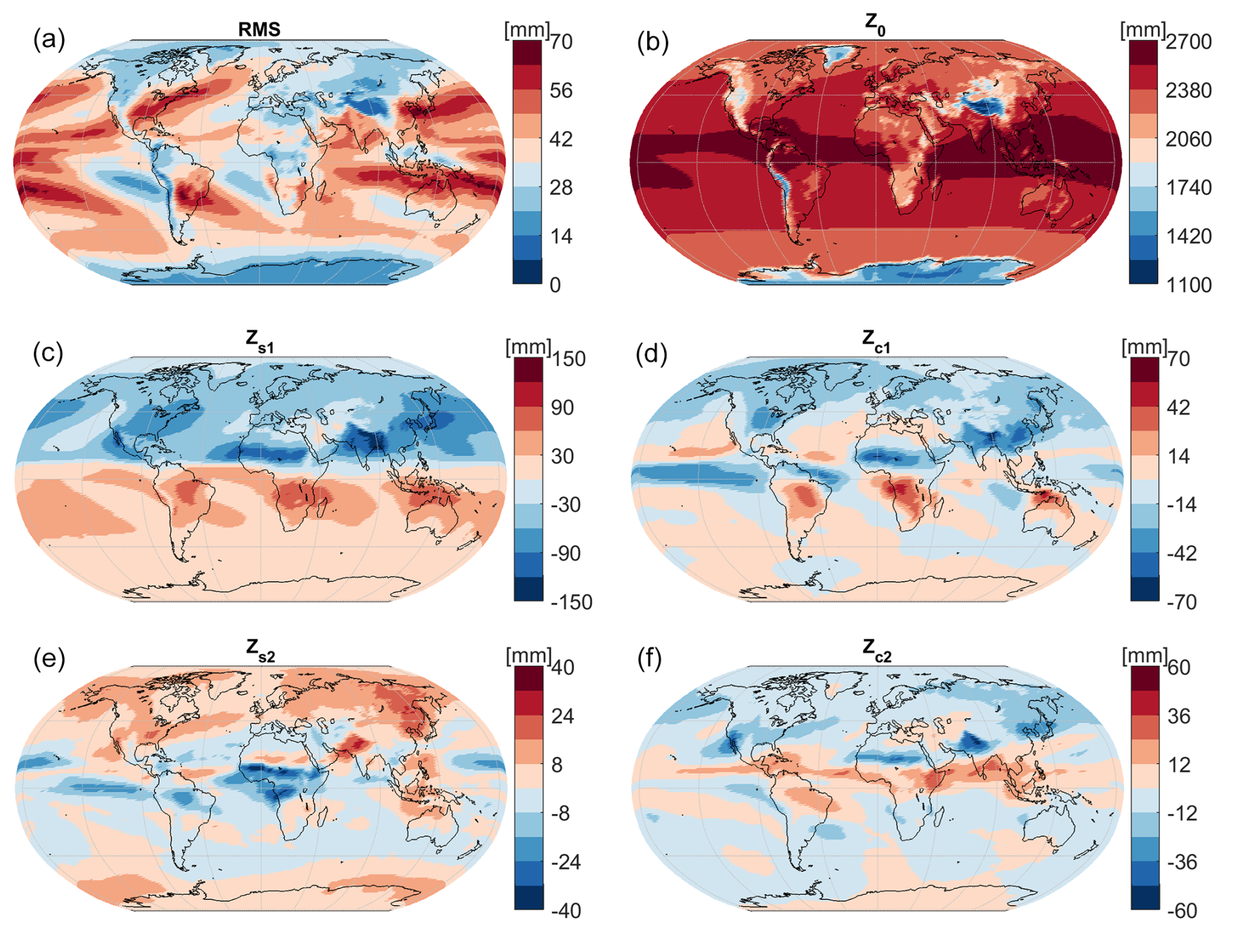
Figure 2 Fitting results of the zenith total delay derived from the VMF global grid product for 2009 to 2018. (a) rms of the ZTD fitting residuals. The remaining subplots give the fitting coefficients of ZTD.

Figure 2 gives the fitting results of the VMF ZTD products in the period 2009–2018. As we do not model the diurnal variation, only the results of epoch 00:00 UTC are considered. The fitting residuals are related to both the altitude and latitude and show regional patterns. On the one hand, the grid points with a higher altitude, e.g., the Tibetan Plateau, the Andes, and the Antarctic, all have a smaller root mean square (rms) value, which is mainly due to the lower water vapor content at such a high altitude. On the other hand, the rms of the fitting residuals also shows a regional pattern. One example is the North Atlantic, where the rms value around the Canary Current on the eastern side is much smaller than that around the Gulf Stream on the western side. The rms value varies from 10 to 70 mm, with 99 % of the grid points within 60 mm (90 % within 50 mm), and the average value is 36.0 mm. As for the average ZTD value, i.e., the Z₀ term, it shows a strong dependence on the latitude and altitude of the grid points, especially the latter, which is mainly due to the distribution of atmospheric pressure. The value varies between 1100 mm in the high-altitude regions and 2700 mm in the tropical regions. The coefficients of the annual term have the opposite pattern in the Northern Hemisphere and Southern Hemisphere, especially the sine term, and those of the semiannual term show more regional patterns.

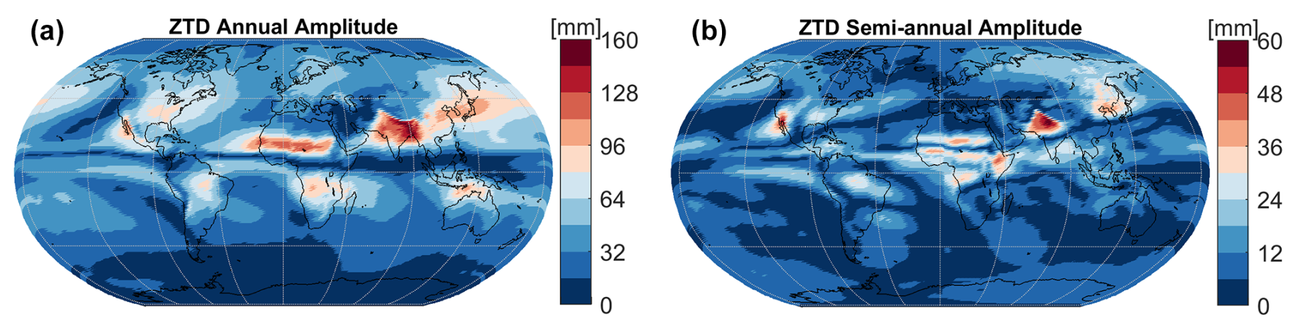
Figure 3 Annual (a) and semiannual (b) amplitudes from the numerical fitting of the NWM-derived ZTD from 2009 to 2018.

Note that we do not fit the ZTD time series with the function of amplitude A and initial phase φ, i.e., $A\cdot \sin (\frac{\mathrm{2}\mathit{\pi }}{\mathrm{365.25}}t+\mathit{\phi })$. The reason is that, without the coefficient of the initial phase, the fitting is numerically more stable. The initial phase and amplitude can always be retrieved given the sine and cosine coefficients, e.g., the annual amplitude using $A_{\mathrm{1}}=\sqrt{s_{\mathrm{1}}^{\mathrm{2}}+c_{\mathrm{1}}^{\mathrm{2}}}$. To better illustrate the annual and semiannual variations of the ZTD, we present the amplitudes of the annual and semiannual terms in Fig. 3. The annual amplitude is less than 160 mm, and large values are observed in the northern Indian subcontinent, between the Sahara and sub-Saharan Africa, and around Japan. The semiannual amplitude is usually within 30 mm in most of the regions, but extremely large values of up to 60 mm also exist that have a similar distribution to those of the large annual amplitudes. The average values of the annual and semiannual amplitudes on a global scale are 34.6 and 9.8 mm, respectively, and the 95 % confidence intervals are 78.4 and 22.2 mm.

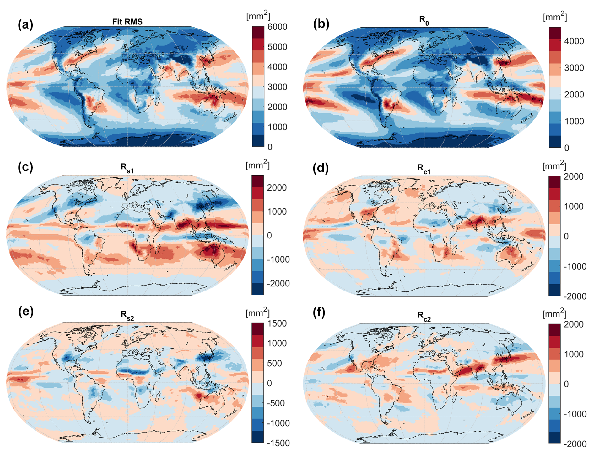
Figure 4 Fitting results of the squared ZTD residuals from 2009 to 2018. (a) Fitting rms. (b) Constant term. (c, d) Sine and cosine coefficients of the annual periodical term. (e, f) Sine and cosine coefficients of the semiannual periodical term. Note the different scales between the different panels.

2.2 Modeling of the ZTD formal error

With the ZTD fitting residuals, i.e., the ZTD from the NWM-derived values minus that from the fitted values, we further model the formal error σ(t) (mm), i.e., the uncertainty information of the empirical delay model, by fitting the squared ZTD residuals Res(t)² using the following equation, which considers constant, annual, and semiannual periodical terms and minimizes the differences between the squared formal error and the squared ZTD residuals.

$$\mathrm{\Delta }=\mathit{\sigma }(t{)}^{\mathrm{2}}-\text{Res}(t{)}^{\mathrm{2}}$$

$$\begin{array}{}\text{(2)}& \begin{array}{rl}\mathit{\sigma }(t{)}^{\mathrm{2}}& =R_{\mathrm{0}}+R_{\mathrm{s}\mathrm{1}}\sin \left({\displaystyle \frac{\mathrm{2}\mathit{\pi }}{\mathrm{365.25}}}t\right)+R_{\mathrm{c}\mathrm{1}}\cos \left({\displaystyle \frac{\mathrm{2}\mathit{\pi }}{\mathrm{365.25}}}t\right)\\ & +R_{\mathrm{s}\mathrm{2}}\sin \left({\displaystyle \frac{\mathrm{4}\mathit{\pi }}{\mathrm{365.25}}}t\right)+R_{\mathrm{c}\mathrm{2}}\cos \left({\displaystyle \frac{\mathrm{4}\mathit{\pi }}{\mathrm{365.25}}}t\right)\end{array}\end{array}$$

Similar to the ZTD modeling, R₀ gives the average value of the squared residuals over a long period, R_s1 and R_c1 are the sine and cosine coefficients of the annual term, and R_s2 and R_c2 are the sine and cosine coefficients of the semiannual term. Δ is the difference between the squared formal error and the squared residuals of the ZTD. Note that their units are all square millimeters given that the unit of the observations, i.e., the squared ZTD residuals Res(t)², is square millimeters. We fit the squared residuals Res(t)² instead of the absolute value of ZTD residuals for the following two reasons. First, the accuracy of tropospheric delay models is always evaluated by the root mean squares of the residuals, and numerically the statistic of absolute residuals is not equivalent to that of the rms of the residuals, which means that a scaling coefficient is required (Chen et al., 2020). Second, in enhancing the GNSS positioning by constraining the tropospheric delay, the weighting of the tropospheric delay which serves as a pseudo observation is based on the squared value of the formal error.

Figure 4 presents the fitting results of the squared ZTD residuals. The constant term R₀ follows the distribution of the rms of the ZTD residuals in Fig. 2, as expected. Interestingly, the fitting accuracy of the ZTD residuals, i.e., Fig. 4a, also follows the distribution of the ZTD residuals. The spatial distribution of the annual and semiannual periodical terms does not show an obvious correlation with the latitude or altitude of the grid points and will be converted into amplitude in the following section and discussed there.

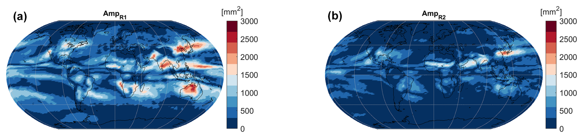
Figure 5 Coefficients of the annual (a) and semiannual (b) amplitudes for the ZTD formal error modeling.

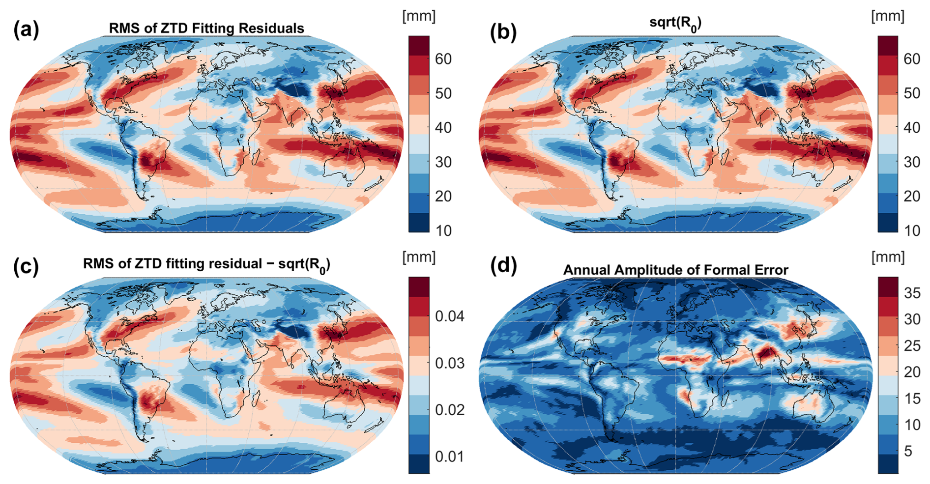
Figure 6 Fitting results of the ZTD formal error. (a) The rms of the ZTD fitting residuals. (b) Average value of the formal error. (c) Difference between the rms of the ZTD fitting residuals and the average formal error. (d) Amplitude of the sine and cosine coefficients of the annual periodical term. The annual amplitude is calculated as half of the peak-to-peak value.

The coefficients of the annual and semiannual amplitudes are given in Fig. 5. The two amplitudes are calculated as ${\text{amp}}_{R\mathrm{1}}=\sqrt{R_{\mathrm{s}\mathrm{1}}^{\mathrm{2}}+R_{\mathrm{c}\mathrm{1}}^{\mathrm{2}}}$ and ${\text{amp}}_{R\mathrm{2}}=\sqrt{R_{\mathrm{s}\mathrm{2}}^{\mathrm{2}}+R_{\mathrm{c}\mathrm{2}}^{\mathrm{2}}}$ (mm²). Note that the presented amplitudes do not give the peak-to-peak values of the empirically modeled formal error and only illustrate the strengths of the annual and semiannual signals. The annual amplitude is rather significant in several regions, such as Northeast China, the central and western parts of Australia, and around the Bay of Bengal (northeastern part of the Indian Ocean). The semiannual amplitudes are smaller than the annual one, the distribution generally follows that of the annual one, and large values are mainly observed in mid- and low-latitude regions such as the East China Sea between China and Japan, northeastern India, and the Arabian Sea between the Indian subcontinent and the Arabian Peninsula.

In Fig. 6, we further compare the rms values of ZTD modeling residuals (Fig. 6a) and the constant term of ZTD formal error (Fig. 6b). Excellent agreement is observed as the differences are negligible (Fig. 6c). The annual amplitude of the formal error is also given (Fig. 6d). The calculation of the annual term does not follow that of the ZTD, as the formal error modeling is based on the squared residuals. Therefore, we simply take half of the peak-to-peak value as the annual amplitude and do not present the semiannual amplitude of the formal error. Note that the unit of the amplitude is millimeters.

As shown in Fig. 6d, the annual amplitude of the formal error shows a correlation with the latitude, and that in high-latitude regions is below 10 mm. The average amplitude is 6.2 mm on a global scale, and 95 % of the grid points are within 16.3 mm. Despite only a few grid points having large amplitudes, the value could still reach up to 30 mm, such as in Northeast China, around the Bay of Bengal (northeastern part of the Indian Ocean), and on the western coast of Africa.

2.3 Modeling the vertical variation of the ZTD

It is well known that the tropospheric delay has a strong dependence on station altitude due to the altitude dependence of atmospheric pressure (Dousa and Elias, 2014; Wang et al., 2022a). Considering that the delays of VMF products refer to a certain altitude of the grid points (shown in Fig. 1), users need to apply the height-related correction. Usually, the first-order exponential function can describe the vertical lapse of tropospheric delay very well, especially for the empirical modeling of tropospheric delay, which aims at an accuracy of several centimeters. A higher-order exponential function could improve the vertical modeling precision further (Wang et al., 2022a), which is not necessary for this work. We adopt the following equation to account for the correction due to the difference between the altitude of the user h and that of the grid point h.

$$\begin{array}{}\text{(3)}& \text{ZTD}\left(h\right)=\text{ZTD}\left(h\mathrm{0}\right)\cdot \exp \left(-{\displaystyle \frac{h-h\mathrm{0}}{\mathit{\beta }}}\right)\end{array}$$

β is the scaling height. In this work we use β = 7.6 km, which is based on the numerical fitting of the NWM-derived ZTD from all grid points in 2009–2018.

As for the modeling of the formal error, it can be easily derived by adopting Eq. (4).

$$\begin{array}{}\text{(4)}& {\mathit{\sigma }}_{\text{ZTD}\left(h\right)}^{\mathrm{2}}={\mathit{\sigma }}_{\text{ZTD}\left(h\mathrm{0}\right)}^{\mathrm{2}}\cdot {\left(\exp \left(-{\displaystyle \frac{h-h\mathrm{0}}{\mathit{\beta }}}\right)\right)}^{\mathrm{2}}\end{array}$$

2.4 Empirical ZTD modeling with uncertainty

Finally, we present the empirical model to provide both zenith delays and the corresponding uncertainty information, which is based on the ZTD from the NWM from 2009 to 2018. The model is based on a 1° × 1° global grid, which has the same altitude as the VMF grid product (https://vmf.geo.tuwien.ac.at/station_coord_files/gridpoint_coord_1x1.txt, last access: 20 February 2025). At each grid point, five coefficients are used to describe the zenith delay, including one for the constant coefficient, two for the annual term, and two for the semiannual terms as shown in Eq. (1). Five coefficients are used to describe the uncertainty, adopting a similar format to the zenith delay. In addition, the correction of the zenith delay and uncertainty caused by station height is based on one lapse rate presented in Sect. 2.3.

To obtain the zenith delay and uncertainty of a location, the user needs to (a) find four grid points around the user given the latitude and longitude, (b) calculate the zenith delays and uncertainties at these four points using the 10 coefficients, (c) apply the altitude corrections for zenith delays and uncertainties using Eqs. (3) and (4) to obtain the values at the user's height, and (d) apply the bilinear interpolation to obtain the values at the user's location.

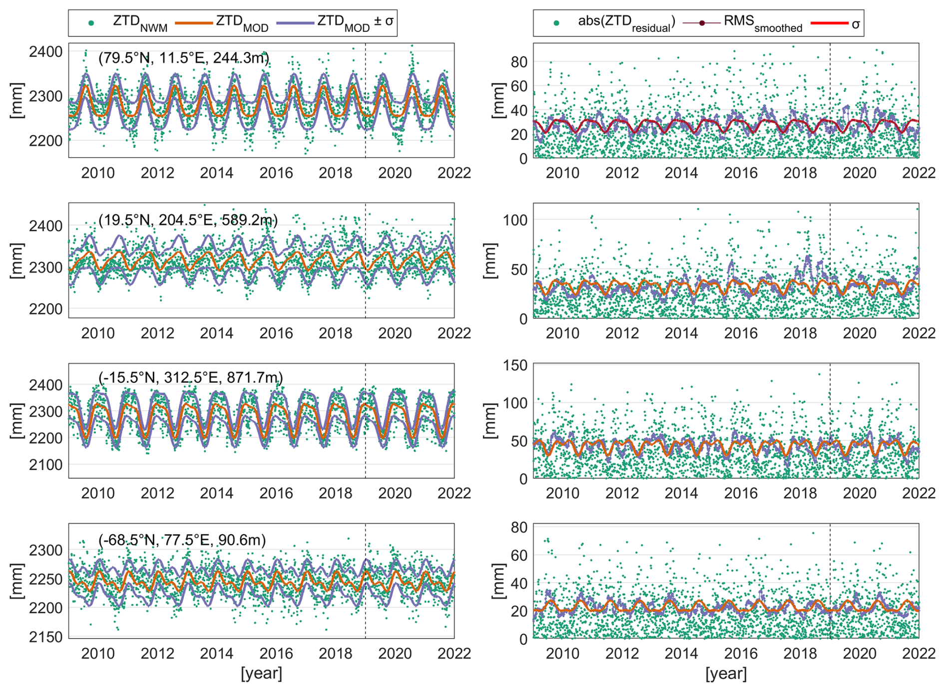
Figure 7 Left: ZTD time series (light-blue dot) and empirically modeled values (red line). The formal errors are given by the blue dashed lines. Right: the absolute value of ZTD residuals (green dots), the smoothed rms of residuals within a period of a 2-month window (green dot line), and the ZTD modeling formal error (red line). The periods for modeling and evaluation are separated by the black dashed line. Note the different vertical scales between the different panels. The locations of all the grid points are given in the left column.

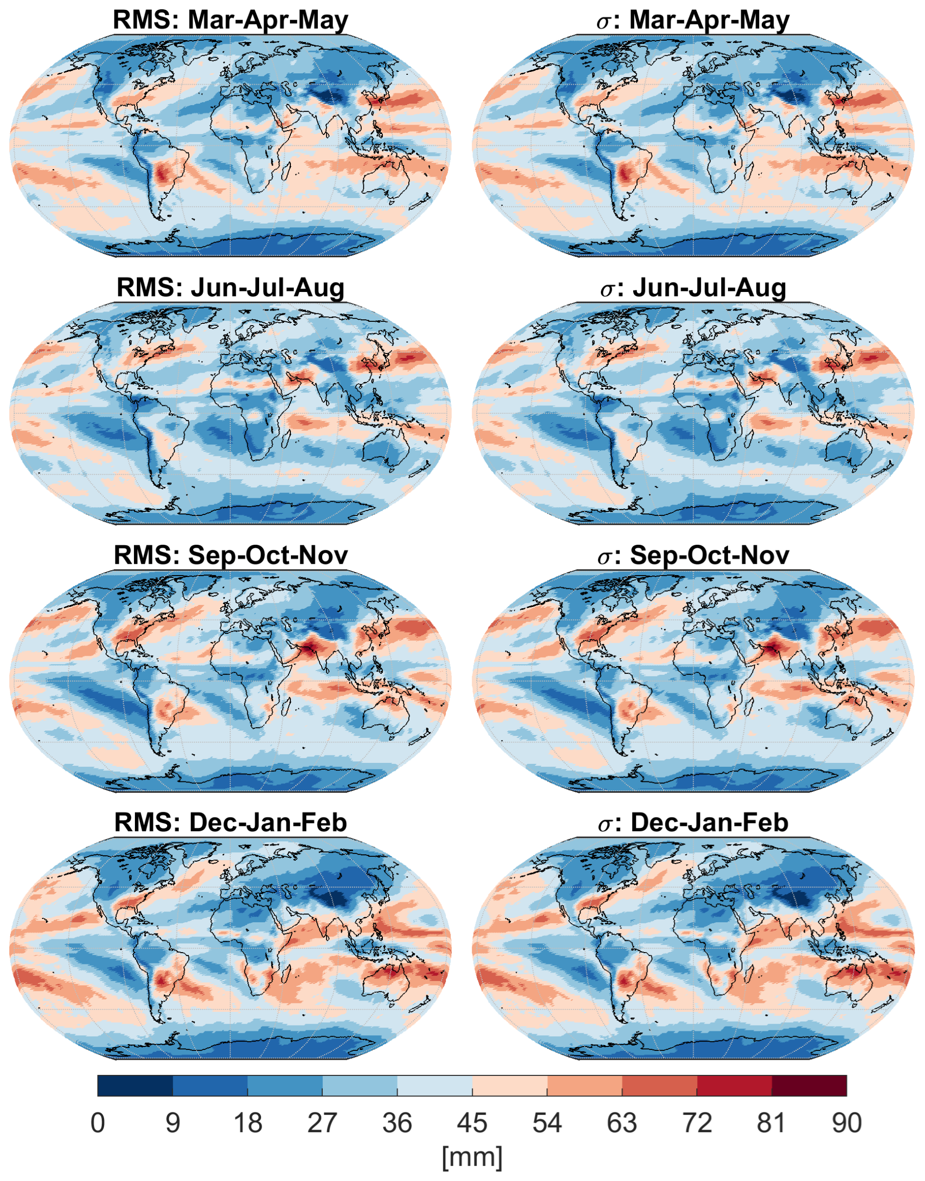
Figure 8 The rms value of the ZTD modeling errors (left column) and the modeling formal errors (right column) in different seasons from 2019 to 2021.

3 Evaluation with NWM products

First, the performance of the empirically modeled ZTD and the formal error is evaluated using NWM-derived ZTD products, i.e., the VMF product. Note that the model is established using the data for the period 2009–2018, and for the evaluation in this section we focus on the period 2019–2021. Figure 7 illustrates the time series at four selected grid points at different latitudes, covering different altitudes. The left column shows that the empirically modeled ZTD agrees well with the NWM-derived values, and the majority of the NWM-derived ZTD values are within the uncertainty line. The annual and semiannual variations of the ZTD are also presented successfully by the empirical model. In the column, the ZTD modeling residuals and the ZTD formal errors are given. The formal error shows good correlation with the residuals at the four grid points, and the ZTD residuals at the upper two grid points show more significant annual variations than the other two grid points. Moreover, for the periods with larger formal errors, i.e., the periods where the formal error has a peak value, the ZTD residuals can be extremely large. The reason is that, for these periods, the water vapor content is more abundant and extreme weather conditions are also more likely to occur. Therefore, extremely large discrepancies are observed. For both the ZTD and the residuals, the agreement between NWM-derived values and empirically modeled ones does not show a significant difference between the modeling period (2009–2018) and the prediction period (2019–2021).

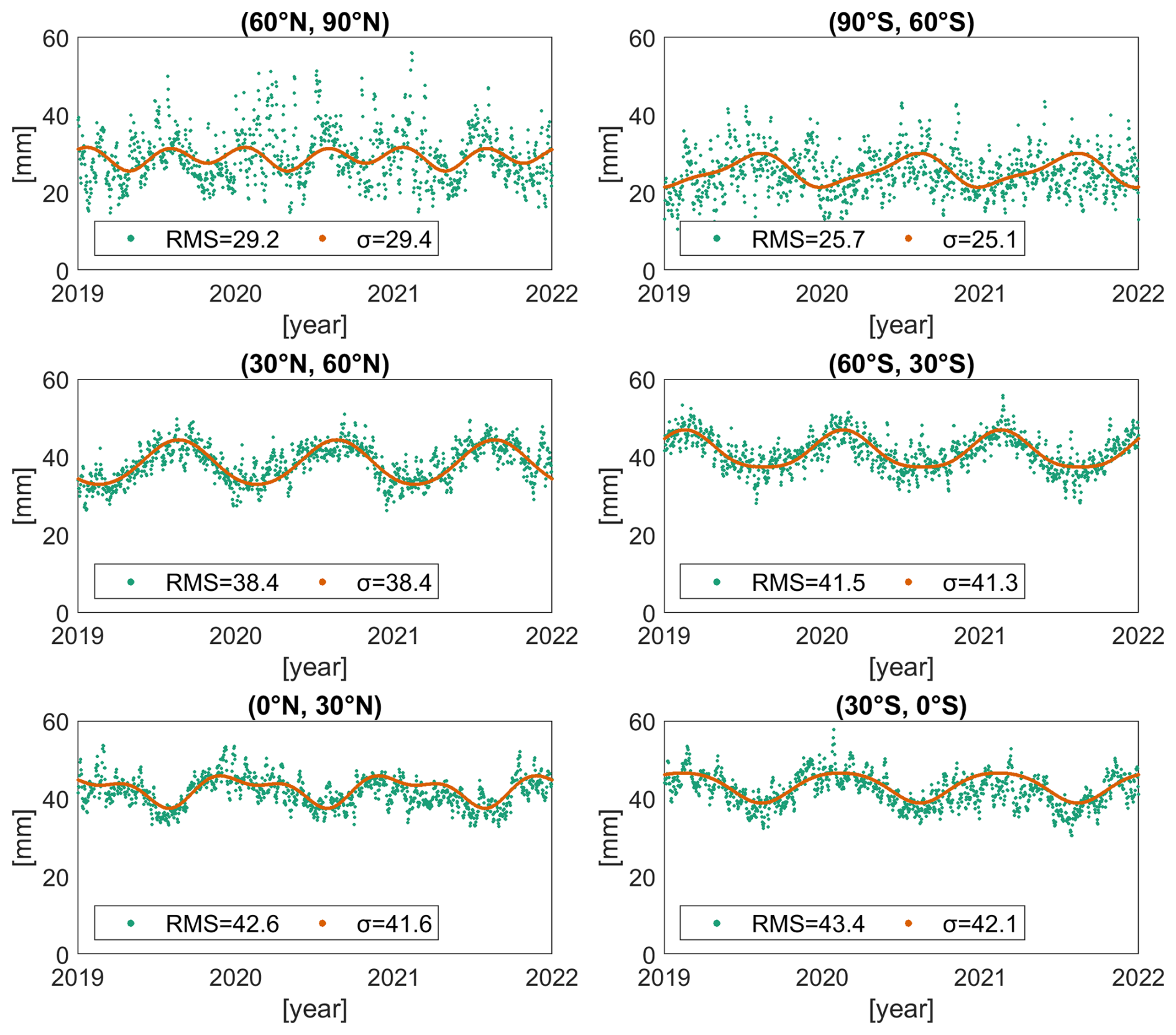
Figure 9 The rms value of ZTD differences between the empirical model and the NWM-derived values, the averaged value of all grid points in different latitude intervals (green dot), and the corresponding ZTD formal errors (red dots). On each day, the average value of all the grid points in the latitude range is presented.

The statistics of the ZTD modeling error in different seasons of the predicted period, i.e., from 2019 to 2021, are provided in the left column of Fig. 8. We also give the corresponding formal errors of ZTD in the right column. The modeling accuracy shows a clear seasonal dependence, and the error is larger in summer, i.e., Jun–Jul–Aug and Dec–Jan–Feb of the Northern Hemisphere and Southern Hemisphere, respectively. In summer, the water vapor content is more abundant, with more rapid variations which cannot be represented accurately using the empirical model, and thus the modeling errors are relatively large. The average rms of all grid points from 2019 to 2021 is 35.3 mm, and the values in March–April–May, June–July–August, September–October–November, and December–January–February are 35.4, 35.0, 35.2, and 35.7 mm, respectively. The formal error shows the same distribution and magnitude as the rms of the ZTD residuals in the four seasons, which demonstrates that the formal error modeling can effectively present the ZTD accuracy with respect to the NWM-derived product. The average values of formal errors in the four seasons are 35.5, 35.1, 35.3, and 35.8 mm, which agrees with the rms of ZTD residuals at the level of 0.1 mm. We also calculate the differences between the rms and the formal error at each grid point, and the maximum discrepancy is only −0.2 mm. Meanwhile, the rms of the differences over all the grid points is less than 0.1 mm.

We further calculate the average values of all grid points within different latitude intervals day by day for both the rms of ZTD residuals and the formal errors, which are presented in Fig. 9. The global grid is divided by a latitude interval of 30°, and on each day we calculate the rms of ZTD residuals from all the grid points together with the average formal error. Except for the region 60–90° N where semiannual signals are also visible, the rms values of ZTD residuals at the other latitudes show significant annual variations, and the formal errors show good agreement. The annual variation in the regions 30–60° N and 30–60° S is larger than that of the other regions, which is mainly caused by the large amplitude of the annual term when modeling formal errors in several locations such as northeastern Asia and central and western Australia (also shown in Fig. 6). Moreover, the rms values of ZTD residuals are smaller at higher latitudes than at lower latitudes, as the latter have more water vapor content, which is more difficult to model empirically. However, the polar regions (latitude higher than 60°), especially around the North Pole, show larger temporal noises than the other regions.

Table 1 Statistics of the ZTD differences between modeled values and NWM-derived values in the prediction period (2019–2021), including the yearly values and the value over the whole period. For each grid point we calculated the mean and rms values, and here we present the average, 95 % of the absolute, minimum, and maximum values of all the grid points (mm).

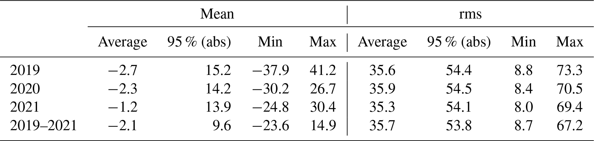
Table 1 summarizes the yearly statistics of the mean and rms values for the prediction period (2019–2021). The year-to-year changes are rather stable, as the average bias varies within 1.5 mm and the average rms varies within 1 mm. On the other hand, the maximum values can vary by up to 10 mm. For example, the maximum bias of all grid points in 2019 is 41.2 mm and that in 2021 is 30.4 mm. This is expected as the minimum and maximum values are more relevant to local severe weathers and can change significantly. The average values indicate that the overall performance of the model is stable in different years.

4 Evaluation with the GNSS ZTD products

In this section, we evaluate the empirical ZTD model using ZTD estimates from GNSS observations. We select 380 IGS stations that have good coverage from 2017 to 2020 (shown in Fig. 1) and use the ZTD estimates from the Nevada Geodetic Laboratory (NGL) product (Blewitt et al., 2018). The NGL tropospheric products are processed with the PPP method using the GipsyX software. The Repro3 final orbit and clock products from the JPL analysis center are fixed. For tropospheric delay modeling, a priori delays and mapping functions are derived from the VMF1 product. The residual ZWD and horizontal gradients are estimated using the random walk processes with a temporal resolution of 5 min, and the corresponding stochastic noises are 5.d-8 and 5.d-9 km s${}^{-\mathrm{1}/\mathrm{2}}$. More details can be found in the data processing strategy description file (http://geodesy.unr.edu/gps/ngl.acn.txt, last access: 20 February 2025). The NGL tropospheric delay products are widely used in tropospheric delay empirical modeling, model evaluation, and comparison with NWM-derived products (Chen et al., 2020; Ding et al., 2022; Pearson et al., 2020; Yu et al., 2021; Yuan et al., 2023). We selected the period 2017–2020 because the modeling is based on the NWM-derived product in the period 2009–2018, and thus the period 2019–2020 is always predicted.

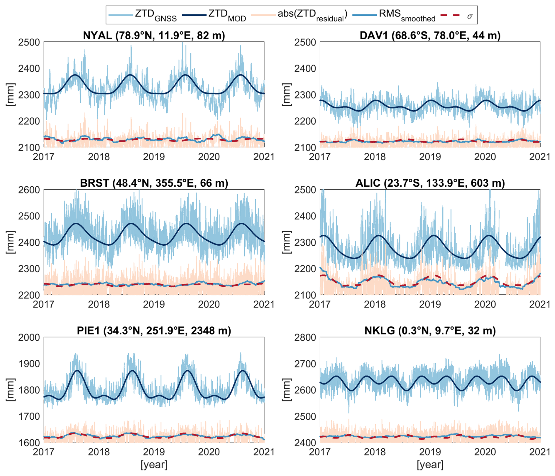
Figure 10 ZTD estimates from the GNSS (ZTD_GNSS) and the empirical model (ZTD_MOD), together with the corresponding residuals (abs(ZTD_residual)). The smoothed rms of ZTD residuals within a 2-month window (RMS_smoothed) and the formal error of the empirical model (σ) are also given. Note that the absolute values of the ZTD residuals are given. The ZTD residuals, rms values, and formal errors are shifted with the same bias for better visibility. The GNSS station names and locations are given in the titles of each panel.

We first use six IGS stations as examples to present the ZTD modeling accuracy, which covers different latitudes and altitudes. Figure 10 gives the ZTD estimates from the GNSS and from the empirical model (in light- and dark-blue lines, respectively). In general, the empirical model can effectively capture the long-term variation of ZTD, mostly the annual and semiannual signals. However, the short-term fluctuations cannot be modeled empirically, leaving large residuals of up to tens of centimeters, especially in summer. The residuals at BRST are larger, and that at DAV1 is smaller, mainly because BRST is located on the coast of France with high water vapor content and DAV1 is located in the Antarctic with lower water vapor content. Note that the ZTD at PIE1 (Pie Town, southwestern USA) is smaller than that at the other stations, due to the higher station altitude.

To inspect the modeling performance of the formal error, we give the absolute values of the ZTD residuals (in light-green lines), i.e., the GNSS estimates minus the empirical modeled values. Depending on the location, the ZTD residuals show different variations. For instance, at station ALIC (central Australia), the residuals show clear annual variations of several centimeters, which is consistent with the modeled amplitude of the formal error in Fig. 6. Station PIE1 also shows annual variations, but the magnitude is much smaller, and the other four stations have no significant annual signals. We further compare the modeled formal error (σ in red dashed line) and the smoothed rms of ZTD residuals (RMS_smoothed in dark-green line), i.e., one rms of the residuals within a period of 2 months. The two values overlap to a large extent, meaning that the modeled formal error agrees well with the residuals.

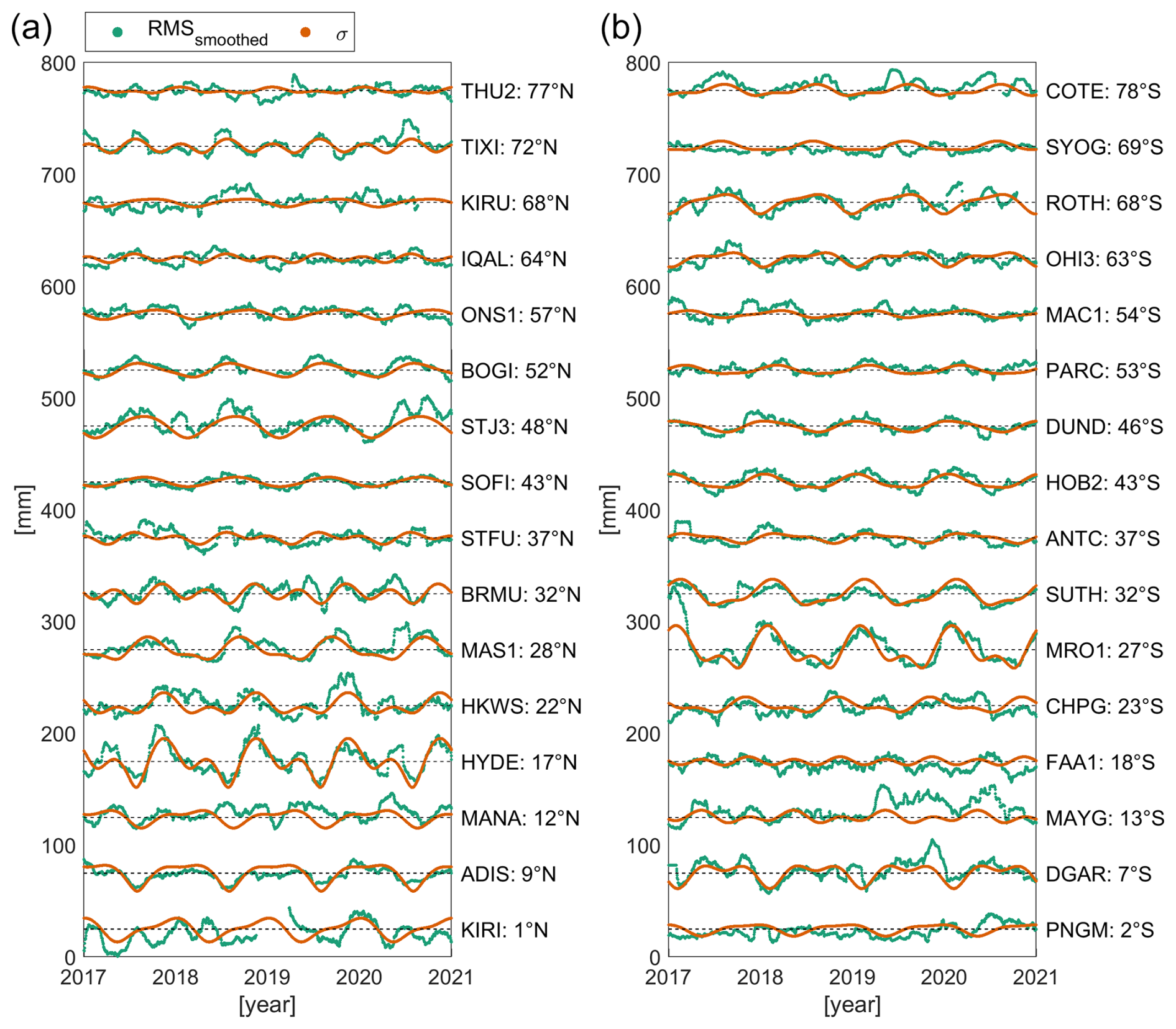
Figure 11 Smoothed rms of ZTD modeling residuals using a 2-month window (green dots) and the formal errors (red dots) at selected GNSS stations. The stations in the Northern Hemisphere and Southern Hemisphere are given in panels (a) and (b), respectively, sorted by latitude. The time series are shifted for better visibility.

The rms values of ZTD residuals within a 2-month period and the formal error at more GNSS stations are presented in Fig. 11. We select one station every 5° in latitude, and in total 32 GNSS stations are given. As shown, the formal error has a very good agreement with the rms of residuals at most of the stations. For stations with a small magnitude of formal error, the fluctuation of the residual rms also tends to be a straight line with some noises instead of showing any annual variations, and for stations with significant annual signals the formal error also shows a very similar pattern. Despite the generally good agreement between the rms of ZTD residuals and the formal error, it is worth mentioning that the short-term noises still exist. For example, at station MRO1 (27° S), the rms is about 30 mm larger than the formal error at the beginning of the year 2017, and at station KIRI (1° N) the rms value could be 20 mm smaller than the formal error in 2017. This is expected, as the rms values present the real accuracy of the empirical model, whereas the formal error can only provide the average value and annual variation based on long-term numerical fitting. The semiannual periodical signals are also significantly visible at several stations, such as BRMU (32° N), HYDE (17° N), MRO1 (27° S), and DGAR (7° S).

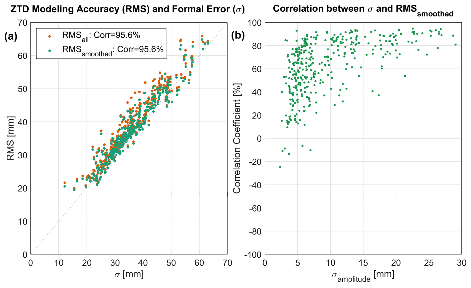
Figure 12 (a) ZTD modeling accuracy (vertical axis) and formal error (horizontal axis) at GNSS stations from 2017 to 2020. For each GNSS station, the rms of all ZTD modeling residuals in 2017–2020 is given by the orange dots (RMS_all), and the average value of all rms values in each 2-month window is given by the green dots (RMS_smoothed). (b) Correlation coefficients between the ZTD formal error and rms of a 2-month time window as a function of the formal error annual amplitude. The correlation coefficients in panel (b) are all statistically significant, with a p value smaller than 0.05.

The agreement between the rms of ZTD residuals and the formal errors is analyzed further in Fig. 12. As shown in the left panel, the agreement is rather optimal and a strong correlation is observed. The correlation coefficient is 96 %, meaning that the formal error can effectively present the accuracy of the empirical ZTD model over the 4 years, i.e., 2017 to 2020. Both the overall rms of the whole period (RMS_all) and the average value of the smoothed rms time series over the 2-month periods show good agreement with the formal error. Taking all the stations into consideration, the average bias of the residual ZTD is −0.4 mm, the mean rms of ZTD residuals is 38 mm, and the mean value of the formal errors is 36 mm.

We also give the correlation coefficients between the smoothed rms of ZTD residuals within a 2-month period and the corresponding formal error in Fig. 12b. For most of the stations, the correlation coefficients are quite large, especially for those with a large annual amplitude of the formal error. The number of stations with magnitudes larger than 20 mm and between 10 and 20 mm are 29 and 103, respectively, and the corresponding average correlation coefficients are 85 % and 77 %. The average value of all the correlation coefficients, including those with negative values, is 63 %, and the median is 70 %. For stations with a small annual magnitude of the formal error, the correlation coefficient is small or even negative. A small magnitude means that the formal error tends to be a straight line, e.g., stations THU2 (77° N), IQAL (64° N), and MAC1 (54° S) in Fig. 11, and thus any discrepancy between the rms of the residuals and the formal error caused by the noise of the rms could degrade the correlation coefficient.

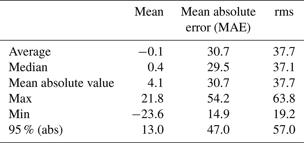
The agreement of the modeled ZTD with respect to GNSS estimates is summarized in Table 2. The model shows no systematic biases as the averaged bias over all the stations is −0.1 mm, despite the fact that the maximum biases can reach up to 2 cm. The average absolute bias is 4.1 mm, which can be attributed to (1) the incorrectly modeled effects at specific stations due to the deficiency of our model that can be improved further by adopting a higher temporal resolution and (2) the systematic biases of GNSS ZTD estimates due to instrument effects (Ding et al. 2023). The rms value varies from 19.2 to 63.8 mm, with an average value of 37.7 mm. Both the bias and rms values agree well with previous investigations of the GPT3 empirical ZTD models and the GNSS ZTD, e.g., an rms of 44.1 mm reported by Ding and Chen (2020) and an rms of 38.56 mm reported by Yao et al. (2024).

Table 2 Agreement of the modeled ZTD with respect to the GNSS estimates. For each station, we calculated the mean, median absolute error (MAE), and rms values of the ZTD differences over the 4 years (2017.00–2021.00), and then the average, median, mean absolute value, maximum, minimum, and 95 % values of all the stations are given (mm).

5 Impact on the convergence time of the kinematic PPP solution

To evaluate the impact of using the empirical ZTD model and the corresponding uncertainty information on GNSS positioning, we perform a pseudo-kinematic PPP solution using the 200 globally distributed IGS stations (shown in Fig. 1) in 2020. The 30 s sampled GPS observations on DOYs 001–030, 091–120, 180–210, and 271–300, which correspond to the four seasons, are processed. On each day, we divide the 24 h data into six arcs and only process 4 h of data per solution. In total, around 720 sessions are processed for each station, depending on the availability of the observations.

The Positioning And Navigation Data Analyst (PANDA) software (Liu and Ge, 2003; Geng et al., 2008) with multi-technique processing developments (Wang et al., 2022b) is used for the data processing. We adopt the conventions in the IGS third reprocessing campaign (Repro3, http://acc.igs.org/repro3/repro3.html, last access: 20 February 2025) for the pseudo-kinematic PPP solutions, where the satellite orbits and clocks are fixed to ESA's Repro3 products. For parameter estimation, we estimate ambiguity as constants per arc, epoch-wise station coordinates, receiver clocks, and zenith tropospheric delays mapped by VMF3. The tropospheric gradients are not estimated as they are not critical for the kinematic PPP accuracy but degrade the convergence speed (Wang and Liu, 2019; Cui et al., 2022). A stochastic processing noise of 5 mm h${}^{-\mathrm{1}/\mathrm{2}}$ is applied to the epoch-wise ZTD estimates. The a priori ZHD is provided by the VMF3 products, and the a priori ZWD is provided by our empirical ZTD model, i.e., the empirical ZTD minus the ZHD from VMF3. Note that it is also possible to adopt other empirical ZHD models, such as the GPT series. The ZWD estimates are constrained to the a priori delay with different weights: 1 m is considered a very loose constraint (solution “No”) and is 1 and 2 times the uncertainty from our empirical model (solutions 1σ and 2σ, respectively). We evaluate both 5 and 15° cutoff elevation angles, which represent ideal and normal cases, respectively. The positioning results are evaluated by comparing them with the IGS Repro3 combined coordinates.

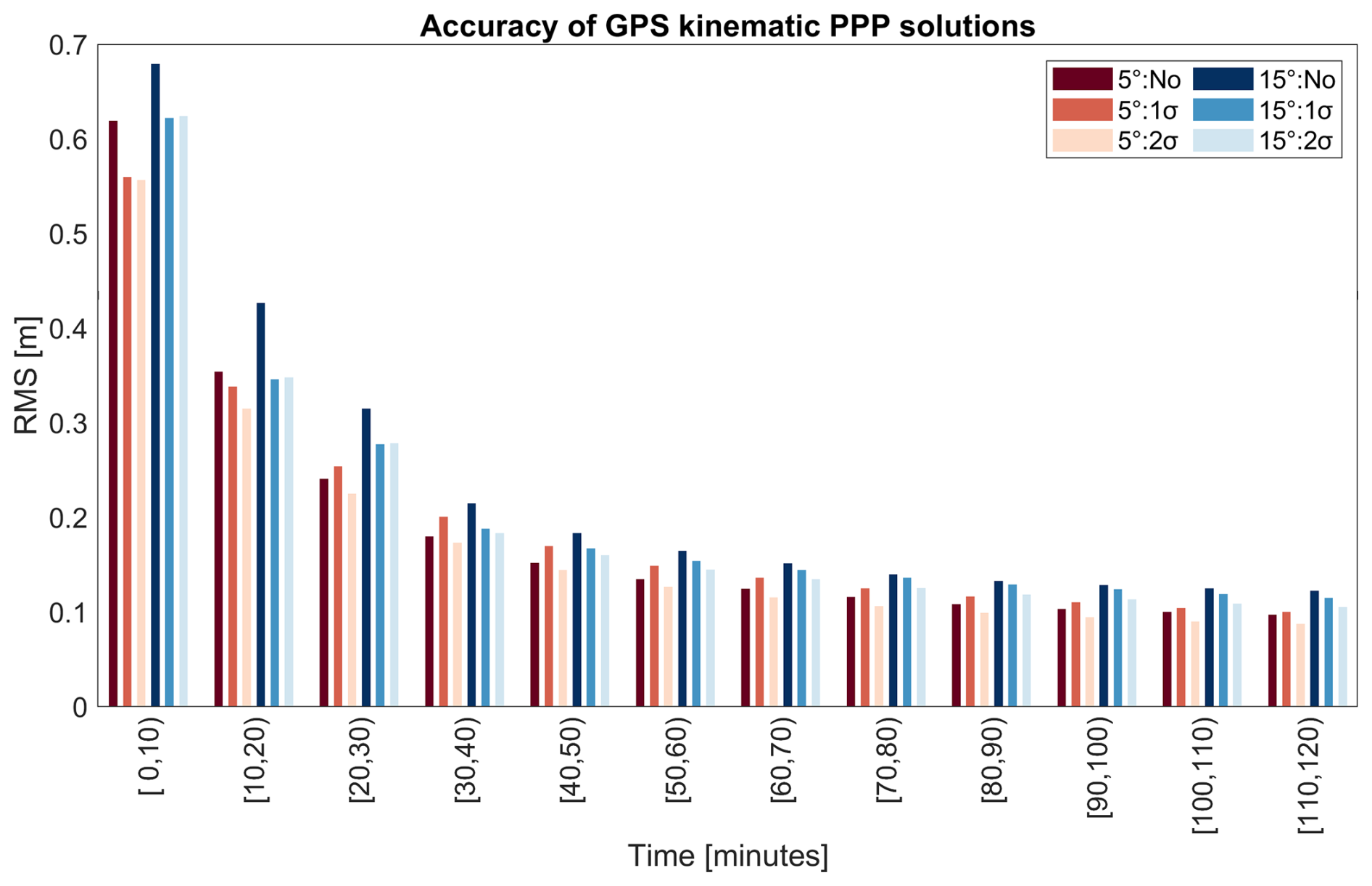
Figure 13 Positioning accuracy of pseudo-kinematic GPS PPP solutions with different constraints on tropospheric delays at different cutoff elevation angles. The rms value in the first 2 h of each solution over a 10 min time window is presented.

Figure 13 presents the rms values of positioning errors in the first 2 h of each solution. Note that we calculate the average rms with a time window of 10 min. In general, applying a proper constraint to the a priori tropospheric delay can improve the positioning performance in the convergence period, i.e., speeding up the convergence time, especially in the first 30 min. For the 15° cutoff elevation angle solutions, both the 1σ and 2σ constraints improve the convergence speed, and the improvement of the first case is less significant after 40 min. As for the 5° cutoff elevation angle solutions, the 1σ and 2σ constraints improve the convergence speed with respect to the loosely constrained solution in the first 20 min, whereas after that only the 2σ solution is improved and the 1σ one is degraded. The positioning results are combined contributions of both real GNSS observations and axillary information, i.e., the external tropospheric delays and the corresponding uncertainties in this case. When the contribution of GNSS observations is less robust, e.g., at the beginning of a session, especially with a higher cutoff elevation angle, the observation geometry is not good enough to provide good estimates, and thus introducing external tropospheric delays and uncertainties contributes to stabilizing the solution and improving the convergence. When a good observation geometry is available, i.e., after the convergence time or with more satellites available, GNSS observation itself can provide robust and accurate coordinates, and the additional tropospheric delay information does not contribute significantly. On the other hand, if a tight constraint is applied, the tropospheric delay error propagates into the coordinates and degrades the solution accuracy.

6 Conclusions and outlook

Empirical tropospheric delay models are important for real-time GNSS applications as they provide precise a priori zenith delays with accuracies of 3 to 4 cm and are easy to implement without any external meteorological input. They serve as both a priori delays and constraints to accelerate the convergence time, and in the latter case uncertainty is required. Currently, most empirical delay models, such as the GPT series, provide only the delay values but not the uncertainty information. As a consequence, users have to numerically test the impact of different values (Yao et al., 2017), which has a dependence on both location and season.

We present a global model to provide both zenith tropospheric delays and the corresponding uncertainties, which facilitates exploitation of empirical delay models in enhancing real-time GNSS applications. Based on 10 years (2009–2018) of NWM-derived zenith delay grids with a spatial resolution of 1° × 1°, we derive the numerically fitted coefficients, which can present ZTD with an accuracy of 36 mm on a global scale. After obtaining the fitting residuals of the delays, we further model the squared residuals using a function containing constant, annual, and semiannual terms, which present the average value and seasonal variations of the uncertainty (formal error). The constant term of the formal error varies between 10 and 60 mm at the different locations, the annual amplitude can reach up to 30 mm, and the global average value is 6.2 mm. Finally, we provide a 1° × 1° global grid, and at each grid point five coefficients are used to present the ZTD and five for the formal error.

To evaluate the proposed model, we use both NWM-derived delays in 2019–2021 and ZTD estimates from 380 GNSS stations in 2017–2020. The comparison with NWM-derived ZTD values shows that the model accuracy is around 35 mm, and the seasonal variations of the ZTD formal error agree with the ZTD accuracy within 0.1 mm on average. The agreement of our empirical ZTD model with GNSS ZTD estimates is 38 mm in terms of the rms statistic, and the average bias is 0.4 mm. The modeled ZTD formal error has a strong correlation with the ZTD accuracy, and the correlation coefficient is 96 %. Inspecting the seasonal variations of the formal error, the stations with a larger annual amplitude of formal error have larger correlation coefficients. For example, for stations with an amplitude larger than 20 mm, the average correlation is 84 %.

Note that our empirical model does not aim for the highest possible modeling accuracy of the delay. Instead, we provide the additional uncertainty information of the delay values to users. On the one hand, the empirical modeling accuracy of zenith tropospheric delay is limited to 3 to 4 cm with the commonly used strategies. This can be verified easily through numerical fitting of the ZTD by the NWM and/or GNSS. Given the NWM-derived ZTD time series, the numerical fitting accuracy of the typical method, i.e., annual and semiannual periodical terms, is around 36 mm (Fig. 2). Considering that the ZTD agreements between NWM and GNSS estimates are around 1 to 1.5 cm (Zhou et al., 2020), the fitting accuracy of the GNSS ZTD is expected to be at the same level (see also Chen et al., 2020). In any case, to achieve better accuracy for the tropospheric delay empirical modeling, more sophisticated methods should be used in the future, such as machine learning and artificial intelligence, which are already utilized in regional tropospheric delay augmentation and water vapor sensing (Miotti et al., 2020; Shehaj et al., 2022; Zhang et al., 2022; Zheng et al., 2022). On the other hand, the uncertainty information is beneficial to real-time GNSS users, especially in scenarios of enhancing convergence speed. As the uncertainty shows large differences between different locations and seasons, it is not optimal to use arbitrary values, and our proposed model can thus provide a realistic reference. As the uncertainty modeling is based on a similar dataset to that of the GPT series, it is also applicable to the GPT series. Therefore, the modeled uncertainty information is also useful for GNSS integrity monitoring, where bounding the residual tropospheric delay is beneficial for vertical alert limits (Lai et al., 2023; McGraw, 2012; Rózsa et al., 2020; Su and Schön, 2022; Yang et al., 2023). For future study, it would also be possible to provide the mapping function modeling error for the empirical mapping functions such as GPT3 and VMF3, whereas how to utilize the uncertainty of mapping functions still needs investigation.