The Water Table Model (WTM) (v2.0.1): coupled groundwater and dynamic lake modelling

Ice-free land comprises 26 % of the Earth's surface and holds liquid water that delineates ecosystems, affects global geochemical cycling, and modulates sea levels. However, we currently lack the capacity to simulate and predict these terrestrial water changes across the full range of relevant spatial (watershed to global) and temporal (monthly to millennial) scales. To address this knowledge gap, we present the Water Table Model (WTM), which integrates coupled components to compute dynamic lake and groundwater levels. The groundwater component solves the 2D horizontal groundwater flow equation using non-linear equation solvers from the C++ PETSc (Portable, Extensible Toolkit for Scientific Computation) library. The dynamic lake component makes use of the Fill–Spill–Merge (FSM) algorithm to move surface water into lakes, where it may evaporate or affect groundwater flow. In a proof-of-concept application, we demonstrate the continental-scale capabilities of the WTM by simulating the steady-state climate-driven water table for the present day and the Last Glacial Maximum (LGM; 21 000 calendar years before present) across the North American continent. During the LGM, North America stored an additional 14.98 cm of sea-level equivalent (SLE) in lakes and groundwater compared to the climate-driven present-day scenario. We compare the present-day result to other simulations and real-world data. Open-source code for the WTM is available on GitHub and Zenodo.

1 Introduction

Over decades to millennia, global climate and hydrological systems jointly modulate the terrestrial water table (Fig. 1). The water table, defined as the surface below which ground is water-saturated, controls both groundwater and lake-water storage volumes (Fan et al., 2007, 2013). The volume of stored water changes over time with water-table elevation as a result of seasonality, human impacts, or longer-term changes in climate and topography. These changes in lake and/or groundwater systems significantly impact the hydrological cycle on a global scale (Ni et al., 2018; Syed et al., 2008).

The upper 2 km of continental crust holds an estimated 22.6×10⁶ km³ of groundwater (Gleeson et al., 2016). This groundwater provides baseflow to rivers and lakes, defines wetland locations (Fan et al., 2013; Zhu and Gong, 2014), and provides a large store of freshwater for human use (Wada, 2016). It also changes over time, with impacts on ecosystems (Amanambu et al., 2020; Cuthbert et al., 2019b; Hu et al., 2017), geochemical cycling (Dean et al., 2018; Ringeval et al., 2010; Zhang et al., 2023b), and sea levels (Konikow, 2011; Pokhrel et al., 2012; Sun et al., 2022; Wada et al., 2012). Meanwhile, although lakes cover only about 3.7 % of the Earth's ice-free land surface (Verpoorter et al., 2014), they are numerous: Verpoorter et al. (2014) recorded over 100 million lakes in their inventory. The total volume of the world's lakes is about 181 900 km³ (Messager et al., 2016). This lake-water storage impacts hydrologic connectivity (Callaghan and Wickert, 2019) and, therefore, also affects sediment and contaminant transport. Surface-water elevation also influences groundwater head and may exert a stronger control on head in gradient-based groundwater models than other factors, including recharge and hydraulic conductivity (Reinecke et al., 2019a). The extent of these water stores highlights the importance of understanding how they change in the long term.

High-performance computing and efficient algorithm design have enabled continental-scale modelling of modern-day groundwater (Fan et al., 2013; Maxwell et al., 2015) and streamflow (Döll et al., 2009; NOAA, 2016). However, we lack models that are capable of global-scale transient simulations lasting decades or longer. These timescales are highly relevant for our understanding of the impacts of changing sea levels and climate on groundwater stores and are of particular importance for understanding changes to the hydrological system over human lifetimes. Existing models that simulate groundwater at large spatial scales allow for either steady-state simulations (Fan et al., 2013; Maxwell et al., 2015) or transient simulations at timescales ranging from hours to a few years (Maxwell et al., 2015; Kollet, 2009; O'Neill et al., 2021). Some hydrologic projections over longer time periods (decades) do exist (Döll et al., 2020; Märker and Flörke, 2003), but these do not explicitly simulate the groundwater table.

Built-in static assumptions and/or equilibrium approaches prevent existing models from adequately considering the possibly of dramatic long-term changes to lake volume, especially when lake extent in the real world is variable. Various land-surface models (e.g. Decharme et al., 2019; Koirala et al., 2014; Lawrence et al., 2019; Wiltshire et al., 2020; Yokohata et al., 2020; Zeng et al., 2002) provide complex depictions of surface and subsurface hydrology. Some include lake components that influence the local climate (Oleson et al., 2010), but they do not incorporate dynamic changes in lake-water storage or lake surface area over time. For example, Müller Schmied et al. (2021) comprehensively simulated surface hydrology, including the dynamics of lake and wetland storage (Döll et al., 2020), but relied on static mapped extents of lakes and wetlands. Many of the aforementioned models also have substantial data input and calibration requirements, complicating the assessment of long-term changes in the water table, which necessarily integrate across timescales for which requisite data are scarce.

To address the challenge of long-term transient simulations of the water table, we present the Water Table Model (WTM). The WTM couples groundwater (Sect. 3) and lake-water (Sect. 4) levels and flow to simulate water-table elevation relative to the land surface across spatial scales ranging from local catchments to the globe and over timescales ranging from months to thousands of years and beyond. By explicitly acknowledging the link between surface-water elevation and groundwater head, the WTM moves beyond the common – but artificial – model truncation at the land surface and instead solves the dynamically linked surface-water–groundwater system (Reinecke et al., 2019a, b). Input data for the WTM are commonly available for both the present day and the recent geological past and are described in Appendix A1.

We designed the WTM with the following goals and philosophies:

1. Simplicity. The focus of the model is on the simulation of the water table alone. Vadose-zone processes, climate, and streamflow are not directly simulated.

2. Computational efficiency. This enables the WTM to be run across hundreds of millions of cells for thousands of years.

3. Open-source model code. The source code for the WTM is available on GitHub (v2.0.1; https://github.com/KCallaghan/WTM/, last access: 30 April 2024) and Zenodo (v2.0.1; https://doi.org/10.5281/zenodo.10611076, Callaghan et al., 2024) for other researchers to use and peruse.

4. Dynamic lakes. Lake locations are not predefined and instead evolve alongside the rest of the water table.

5. Broad applicability. The WTM can be used across a broad range of spatial scales, from catchments to global scales, and can produce both transient and steady-state water-table outputs.

In order to enable long-term, large-scale simulations of both the groundwater table and dynamic lake surfaces, the WTM makes use of Fill–Spill–Merge (FSM) (Barnes et al., 2021), a highly efficient computational tool for routing water across land surfaces and into depressions. The treatment of surface water in FSM allows us to evaluate surface-water storage with long time steps, neglecting detailed simulations of cell-to-cell river flow. For groundwater, we solve the 2D horizontal groundwater flow equation for saturated flow in an unconfined aquifer, as discussed in Sect. 3. This follows the saturated-type conceptual approach to groundwater simulation, as classified in Condon et al. (2021). By focusing only on 2D horizontal saturated flow, our formulation is simplified enough to enable large-scale (continental) and long-term (monthly to millennial) simulations, which is our aim.

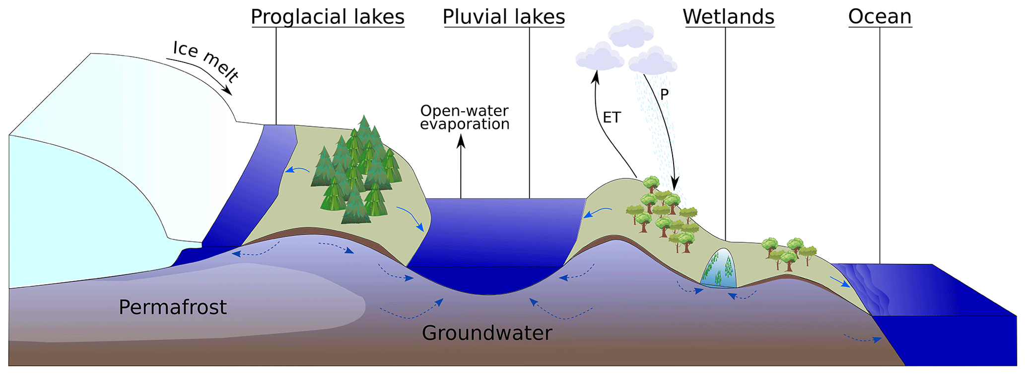
Figure 1 The water table, incorporating groundwater and lake surfaces, is an integral part of the global hydrologic system, interacting with all other major hydrologic stores, including ice, the ocean, and the atmosphere. In this figure, the solid blue arrows indicate the direction of surface-water flow, and the dotted darker-blue arrows indicate the direction of groundwater flow. ET: evapotranspiration. P: precipitation.

2 Model summary

The WTM (Callaghan et al., 2024) simulates water-table elevation relative to the land surface (here referred to as the relative water-table elevation, z_wr), including both groundwater and dynamically changing lake surfaces. The water table is controlled by sea levels and topography, as well as by water inputs (precipitation and ice melt) and outputs (evapotranspiration and open-water evaporation). Groundwater flow is dependent on local hydraulic conductivity, discussed further in Sect. 3.2, and slows in permafrost regions. The WTM is implemented in C++. The code can be acquired from GitHub (https://github.com/KCallaghan/WTM) and Zenodo (v2.0.1; https://zenodo.org/records/10611076).

Within the WTM, separate model components for the simulation of groundwater (Sect. 3) and dynamic lakes (Sect. 4) are run sequentially in a repeated cycle to allow for feedback between groundwater and surface water in the terrestrial hydrological system (see Fig. 2). Both the groundwater and dynamic lake components use the same sets of input data and modify the same water-table array to produce one final water table, with groundwater represented as negative z_wr values and lakes as positive z_wr values. Any water that exfiltrates during the groundwater step is moved downslope into lakes or the ocean during the surface-water step; conversely, seepage from lakes may occur during the surface-water step, and lake water is included in the hydraulic head field used to calculate groundwater movement. The steps followed within the model are visualised in Fig. A1.

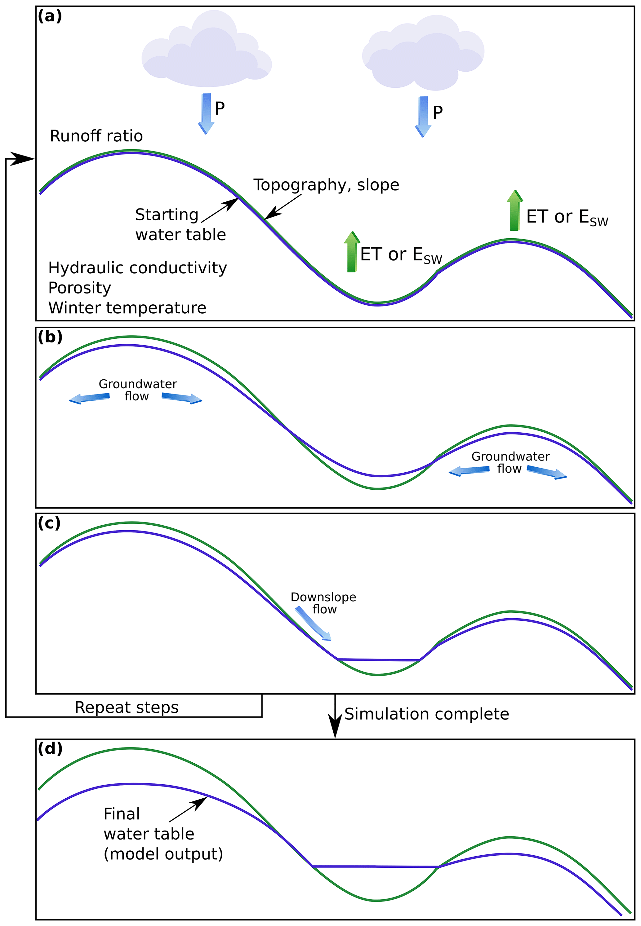
Figure 2 A schematic of the WTM. (a) A cross section of a hypothetical portion of a landscape, including hillslopes and a depression that may hold a lake. Inputs to the WTM include precipitation (P); evapotranspiration (ET); surface-water evaporation (E_SW), used in place of ET when lakes are present; topography; the topographic slope; the runoff ratio; hydraulic conductivity; porosity; and winter temperatures. A starting water table may be provided, or for steady-state runs, the water table is initialised at the land surface. (b) The groundwater component executes, and groundwater flow modifies the water table. Here, the water table is deeper below the hilltops, and exfiltration has occurred on the hillsides. (c) FSM (the dynamic lake component) has been executed. Surface water is now distributed from hillslopes into lakes situated at the bottom of depressions. The steps in panels (a) to (c) repeat until the user-defined number of time steps have been completed. (d) The simulation is complete, and the resulting water table is saved to a file.

The WTM captures broad natural patterns in water-table elevations. Its simplified treatment of groundwater flow makes it most appropriate for large spatial scales, ranging from continent-spanning catchments to the globe. Additionally, the WTM's assumption that surface water always completes its travel to depressions or the ocean makes this model most appropriate for long temporal scales, ranging from months to millennia. The WTM can be used to simulate both transient and steady-state water-table conditions for any given set of input data. For steady-state model runs, the user must run the model for long enough to allow the water table to equilibrate to the given topography and climate. If users wish to monitor changes in the water table, values indicating the total change in the array are saved to a text file, and the full water table is saved at user-defined intervals. For transient runs, the user simply selects the amount of time for which to run the simulation and provides input data at the start and end points of the simulation. The methodology for both transient and steady-state simulations is broadly the same, with the only practical difference being the possibility of topographic and climatic changes over time, which may occur in the case of the transient model run. The input data required by the WTM are listed in Appendix A1. As an output, the WTM returns a 2D array (z_wr), which corresponds to the water-table elevation minus the land-surface elevation (positive values indicate exposed surface water, while negative values indicate groundwater).

3 The groundwater component

3.1 Computing the groundwater table

We compute the groundwater table at each time step using the 2D horizontal groundwater flow equation (Eq. 1) for saturated groundwater flow in an unconfined, heterogeneous aquifer (Freeze and Cherry, 1979). This method applies the Dupuit–Forchheimer approximation, which assumes that flowlines are horizontal and that the hydraulic gradient is equal to the slope of the water table and does not vary with depth below the water table. These assumptions are valid when the slope of the water table is small (Freeze and Cherry, 1979), which is usually the case at the spatial resolutions used in the simulations in Sect. 6.

$$\begin{array}{}\text{(1)}& S_{\mathrm{y}}{\displaystyle \frac{\partial h}{\partial t}}={\displaystyle \frac{\partial }{\partial x}}\left(T{\displaystyle \frac{\partial h}{\partial x}}\right)+{\displaystyle \frac{\partial }{\partial y}}\left(T{\displaystyle \frac{\partial h}{\partial y}}\right)+R\end{array}$$

Here, we solve for h, the groundwater head. T is the transmissivity (depth-integrated hydraulic conductivity; see Sect. 3.2). Moreover, t represents time, and x and y are the two dimensions of groundwater movement. R represents recharge; details on how values for R are selected are given in Sect. 3.3. S_y is the specific yield, here approximated as being equal to the porosity and provided as input data by the user.

To solve Eq. (1), we use the Scalable Nonlinear Equations Solvers (SNES) component of the Portable, Extensible Toolkit for Scientific Computation (PETSc) (Balay et al., 1997, 2022a, b) in C++. Full details on the discretisation and implementation of this equation are given in Appendix B. In the simulations included within this paper, we use the Anderson (1965) mixing method (selectable at runtime), which iteratively solves non-linear equations, to compute the groundwater head, h, at regular time intervals. Converting h to the relative water-table elevation, z_wr, is trivial and expressed as follows: $z_{\mathrm{wr}}=z+h$, where z is the elevation of the land surface.

3.2 Transmissivity

Transmissivity (T), the depth-integrated hydraulic conductivity from −∞ to z_wr, is needed to solve for groundwater flow (see Appendix B). To obtain T, we require knowledge of the hydraulic conductivity values throughout the entire depth of the aquifer. Data on variability in hydraulic conductivity with depth are not available at the spatial scales we assess here, so we follow the common assumption that this value decreases exponentially with depth (Ameli et al., 2016; Cardenas and Jiang, 2010; Fan et al., 2013). Users provide a single near-surface hydraulic conductivity value for each cell of the domain, which is used from the land surface to a depth of 1.5 m because global soil datasets are representative of conditions up to approximately this depth. We refer to this value as K_1.5. Beyond depths of 1.5 m, hydraulic conductivity decays exponentially from this near-surface value.

We specify the rate of this exponential decay using an e-folding depth (f_d). The local terrain slope is used as a modifier: steeper slopes support less sediment, so hydraulic conductivity decays more rapidly. A temperature-dependent modifier (T_f) further decreases the e-folding depth at locations where seasonal frost or permafrost occurs. Accordingly, f_d is expressed as

$$\begin{array}{}\text{(2)}& f_{\mathrm{d}}=f\times T_f,\end{array}$$

where f is the slope-dependent term, defined as

$$\begin{array}{}\text{(3)}& f=max\left(f_{\min },{\displaystyle \frac{a}{\mathrm{1}+bS}}\right),\end{array}$$

where S is the terrain slope, and a, b, and f_min are user-selected calibration constants.

T_f is incorporated into the e-folding depth following the method and temperature ranges used by Fan et al. (2013). When the average winter temperature drops below −5 °C, we assume that seasonal frost inhibits groundwater flow. When average winter temperatures fall below −14 °C, we assume that groundwater flow is affected by permafrost. This limits lateral drainage, reducing the effective hydraulic conductivity (Fan and Miguez-Macho, 2011). We define T_f as

$$\begin{array}{}\text{(4)}& T_f=\left\{\begin{array}{l}\mathrm{1}\\ \text{if }(T_{\mathrm{C}}>-\mathrm{5}\mathrm{°}\mathrm{C}),\\ \mathrm{1.5}+\mathrm{0.1}{T}_{\mathrm{C}}\\ \text{if }(-\mathrm{14}\mathrm{°}\mathrm{C}<T_{\mathrm{C}}<-\mathrm{5}\mathrm{°}\mathrm{C}),\\ max(\mathrm{0.17}+\mathrm{0.005}{T}_{\mathrm{C}},\mathrm{0.05})\\ \text{if }(T_{\mathrm{C}}<-\mathrm{14}\mathrm{°}\mathrm{C}),\end{array}\right.\end{array}$$

where T_C is the temperature in degrees Celsius.

With this hydraulic conductivity structure in hand, we calculate the transmissivity. We consider three possible cases:

1. The water table lies below 1.5 m depth, where the exponential decay of hydraulic conductivity comes into play. In this case, we must use the f_d values computed earlier.

2. The water table lies in the shallow subsurface, above 1.5 m depth, where the unmodified hydraulic conductivity from our input data is representative of conditions at the water table.

3. The water table lies above the land surface. In this case, hydraulic conductivity is calculated at the level of the land surface (i.e. it is identical to that for a fully saturated substrate). The dynamic lake component (Sect. 4) later moves the surface water into depressions or out of the domain as appropriate.

Based on these three cases for hydraulic conductivity, we follow the methods used by Fan et al. (2013) to calculate transmissivity as follows:

$$\begin{array}{}\text{(5)}& T=\left\{\begin{array}{l}{f}_{\mathrm{d}}\times K_{\mathrm{1.5}}\times \exp \left(\frac{z_{\mathrm{wr}}+\mathrm{1.5}}{f_{\mathrm{d}}}\right)\\ \text{if}(z_{\mathrm{wr}}<-\mathrm{1.5}\text{ m})\left(\text{deep subsurface}\right),\\ K_{\mathrm{1.5}}\times (z_{\mathrm{wr}}+\mathrm{1.5}+f_{\mathrm{d}})\\ \text{if}(-\mathrm{1.5}\text{m}\le z_{\mathrm{wr}}\le \mathrm{0}\text{m})\left(\text{shallow subsurface}\right),\\ K_{\mathrm{1.5}}\times (\mathrm{0}+\mathrm{1.5}+f_{\mathrm{d}})\\ \text{if}(\mathrm{0}\text{m}<z_{\mathrm{wr}})\left(\text{above surface}\right),\end{array}\right.\end{array}$$

where T is the transmissivity, f_d is the e-folding depth (Eq. 2), K_1.5 is the shallow-subsurface horizontal hydraulic conductivity (assumed valid to a depth of 1.5 m), and z_wr is the relative water-table elevation. See Fan et al. (2013) for more information on the derivation of these formulae.

3.3 Recharge and evaporation

We use the climatic water input (W_in, including precipitation and any other incoming water, such as ice melt), overland evapotranspiration (ET), and open-water evaporation (E_SW) input arrays (see Appendix A1 for a full list of all required input arrays), along with the optional runoff ratio array (r_r), to determine how much water is available to recharge the groundwater table and how much surface water will evaporate.

When surface water is present, evaporation rates typically increase. Physically, this is because actual evaporation can equal potential evaporation at these locations. Both physically and algorithmically, the increased rate of evaporation typically acts as a feedback that slows runaway lake growth by decreasing the catchment-wide water balance as the lake surface area increases. If lake water is present in a cell, then sufficient evaporation can remove water from the cell. In cells that do not contain lakes, sufficient evapotranspiration can result in no water being available to add to the groundwater; however, the Earth's surface shields the groundwater itself from evaporation. To account for changes in evaporation dependent on the presence of surface water, the WTM recalculates the total water input to each cell (Eq. 6) at the beginning of each groundwater–surface-water model cycle. This total water input (W_tot) is given by

$$\begin{array}{}\text{(6)}& W_{\mathrm{tot}}=\left\{\begin{array}{l}max(W_{\mathrm{in}}-\mathrm{ET},\mathrm{0})\\ \text{if}{z}_{\mathrm{wr}}\le \mathrm{0}\left(\text{subsurface}\right),\\ W_{\mathrm{in}}-E_{\mathrm{SW}}\\ \text{if}{z}_{\mathrm{wr}}>\mathrm{0}\left(\text{above surface}\right).\end{array}\right.\end{array}$$

Optionally, a user can provide a spatially distributed runoff ratio (r_r), which sets the proportion of incoming water that runs off over the land surface rather than infiltrating into the subsurface. This runoff is routed over land via the dynamic lake component of the model, discussed in Sect. 4, and the remaining water is treated as local recharge and applied to the water table. If unassigned, r_r=0 by default.

The amount of runoff, r, in each cell where W_tot>0 is expressed as

$$\begin{array}{}\text{(7)}& r=r_{\mathrm{r}}{W}_{\mathrm{tot}}.\end{array}$$

As its complement, recharge is defined as

$$\begin{array}{}\text{(8)}& R=W_{\mathrm{tot}}-r.\end{array}$$

Equation (8) indicates that the WTM neglects unsaturated-zone processes. We made this design decision for three reasons. First, we sought to maintain the simplicity of the modelling framework in order to understand and interpret its results. Second, the timescale of unsaturated-zone processes becomes increasingly negligible with longer-term simulations (Sousa et al., 2013), so we chose to neglect these processes in the multi-millennial-scale simulations we include here. Third, and most importantly, simulating the unsaturated zone is computationally expensive (Maxwell et al., 2015) and prohibits the multi-millennial, continental-scale model runs presented in this work.

4 The dynamic lake component

The dynamic lake component uses a parsimonious graph-based approach to move surface water into depressions and to compute surface-water storage within these depressions. Depressions are defined as inwardly draining regions within the topography, where water would naturally pool without being able to flow away. The dynamic lake component proceeds in two steps:

1. It computes a depression hierarchy (Barnes and Callaghan, 2020) based on an input digital elevation model (DEM).

2. It uses the Fill–Spill–Merge method – modified to include lake seepage and, optionally, infiltration – to rapidly allocate runoff to these depressions (Barnes et al., 2021) and to calculate the resulting depth of surface water in all of the depressions.

4.1 The depression hierarchy

Understanding the topological and geographical relationships between depressions in the landscape allows us to more rapidly calculate how these depressions will trap and store water. An unfilled depression will retain water that flows into it, while a depression that is already filled with water will overflow either to another depression or to the ocean. The depression hierarchy algorithm builds the depression hierarchy data structure (Barnes and Callaghan, 2019) by analysing the input topography to determine the locations of internally drained depressions and their catchments. We use this data structure (for a full description, see Barnes and Callaghan, 2019, 2020) to compute surface-water flow using Fill–Spill–Merge, as discussed in Sect. 4.2. The depression hierarchy is scale-independent, though the accuracy of the computed depression network depends on the quality and resolution of the input DEM. For the implementation of the depression hierarchy used in this work, we modified the code described by Barnes et al. (2020) in two critical ways: we relaxed the assumption of a uniform grid-cell size, and we added a parameter to account for groundwater storage in each cell.

4.1.1 Latitude-dependent variable cell areas

When performing computations using geospatial data represented on a latitude–longitude grid, cells at higher latitudes have smaller areas than cells at lower latitudes due to the roughly spherical shape of the Earth. Therefore, we generalise the code to allow for latitude-dependent variable cell sizes (Callaghan et al., 2024). This modification is crucial for our ability to conserve water volume as water moves from cell to cell.

4.1.2 Groundwater storage

Here, we modify the depression hierarchy to record the volume available for water storage below the land surface in a given depression (i.e. the groundwater space below cells that may receive an influx of surface water). This allows the algorithm to more accurately assess the total capacity for water storage in each depression. This change was necessary for the WTM because we consider both surface and groundwater. When the water table is below the land surface, we assume that the ground becomes saturated before surface water begins to fill the depression.

4.2 Fill–Spill–Merge algorithm

The WTM computes lake levels using the Fill–Spill–Merge (FSM) algorithm (Barnes and Callaghan, 2020; Barnes et al., 2021). In this work, we modify the original FSM algorithm from Barnes et al. (2021) by adding optional infiltration (Sect. 4.2.1), implementing seepage from lake cells (Sect. 4.2.2), and allowing cell size to vary with latitude (Sect. 4.2.3).

FSM rapidly routes surface water downslope into depressions using a depression hierarchy (Barnes et al., 2020) (Sect. 4.1). If a depression has been filled by precipitation or runoff to the point where it cannot contain any more water, it will spill, sending any additional water to its neighbouring depression. If two neighbouring depressions are both filled, they will merge to form a larger meta-depression, which will then continue to fill with water. This process continues until all surface water has flowed to either a depression or the ocean. This combination of the depression hierarchy and FSM solves the aforementioned flow-routing and water-distribution problem thousands of times faster than previous models (Barnes and Callaghan, 2019; Barnes et al., 2021).

FSM is time-independent, always moving surface water to its final destination in depressions, to the ocean, or out of the model domain within a single time interval. We apply this process in the WTM under the assumptions that surface-water movement is fast in comparison to groundwater movement and that only equilibrated surface-water results are needed over the timescales we address using the WTM. Overland flow, including streamflow, is implied through the calculation of flow directions and the final locations of standing water but is not explicitly modelled. The output of FSM is an array of the z_wr result after infiltration has occurred (optional) and surface water has completed flow into depressions to form lakes or exited the domain.

4.2.1 Infiltration

Here, we add an optional infiltration component to FSM. When the infiltration option is enabled, the FSM algorithm first moves surface water downslope, cell by cell, using the flow directions generated by the depression hierarchy. As the water moves downslope, some may undergo infiltration; the remainder continues along the flow path until it flows either into the ocean, out of the domain, or into a pit cell (that is, the cell within a depression that has the lowest elevation).

When the infiltration option is disabled, the land surface is treated as impermeable in order to simulate the rapid evacuation of surface water from each cell via river networks. To speed up calculations, the algorithm skips cell-to-cell water flow and instead uses the depression hierarchy data to move water directly from each surface-water-containing cell to the relevant depression in the hierarchy.

Our method for managing infiltration considers the vertical hydraulic conductivity within the cell, the travel time of water across the cell, and the amount of unsaturated below-ground space in the cell that can potentially accommodate infiltrating water. For full details on the method used, see Appendix C. Here, we summarise the amount of infiltration (I) that occurs in a cell with the following equation:

$$\begin{array}{}\text{(9)}& I=min\left(-\mathit{\varphi }{z}_{\mathrm{wr}},I_{\mathrm{pot}}\right),\end{array}$$

where infiltration (I) corresponds to the minimum value of the amount of unsaturated below-ground space (or subsurface porosity, ϕ), multiplied by the negative relative water-table elevation (−z_wr), and the maximum potential infiltration (I_pot) that could occur in the cell. I_pot is defined as

$$\begin{array}{}\text{(10)}& I_{\text{pot}}=\left\{\begin{array}{ll}{h}_{\mathrm{0}}& \text{if }{h}_{\mathrm{0}}^{\mathrm{5}/\mathrm{3}}\le \frac{\mathrm{5}}{\mathrm{3}}\frac{n}{S^{\mathrm{1}/\mathrm{2}}}{k}_{\text{sat}}\mathrm{\Delta }L,\\ k_{\text{sat}}{t}_I& \text{otherwise},\end{array}\right.\end{array}$$

where h₀ is the initial height of the water entering the cell; n is the Gauckler–Manning coefficient, here set to a default value of 0.05 m${}^{-\mathrm{1}/\mathrm{3}}$ s; S is the slope; k_sat is the infiltration rate; and t_I is the transit time taken by water to cross the cell.

Use of the infiltration module is only recommended for cases in which the input data have a high enough resolution to resolve hillslopes and river channels that fully occupy distinct individual cells. When using coarser-resolution input data, a single pixel ultimately contains sections of both the river network and hillslope, and the model does not have sufficient information about the transit routes and times of water across these different zones – determined by drainage density and hillslope geometry – to realistically simulate infiltration. When the input data resolution becomes high enough to differentiate between the hillslope and channel components of the landscape, the infiltration component adds an additional element of realism to the model.

4.2.2 Seepage

When a lake is present in a depression, we allow the water column to instantaneously seep into the subsurface until either (a) the entire subsurface is saturated or (b) no surface water remains. The WTM does not simulate any perched water tables; the lake surface represents the water table, with complete saturation occurring up to that elevation.

4.2.3 Variable cell areas

As mentioned in Sect. 4.1.1, cell areas for unprojected geospatial data can vary dramatically based on latitude. The same volume of water at two different latitudes would translate to different heights of groundwater or surface water in a cell. As with the depression hierarchy, we account for this variable cell area when calculating z_wr, allowing us to conserve water volume within the model.

5 Computational performance

In a scaling test, we found a scaling of approximately 𝒪(n²) between the runtime and the number of cells in the domain. Our test used several square-sized datasets from the GEBCO_2020 dataset (GEBCO Bathymetric Compilation Group, 2020), with the smallest dataset covering 54–55° N, 102–103° W, and the largest dataset covering 43–73° N, 74–104° W (northeastern North America). We used uniform values for other input data (precipitation, evapotranspiration, porosity, hydraulic conductivity, and winter temperature). All tests used a spatial resolution of 30 arcsec. Scaling tests were run on a desktop computer with an Intel^® Core™ i9-10900 (2.80 GHz) processor, featuring two threads per core, 10 cores per socket, and 134 GB of RAM. For larger datasets, such as those shown in Sect. 6, high-performance computing (HPC) is recommended.

In this scaling test, the SNES convergence tolerance (stol) was set to 10⁻⁶, and the Anderson (1965) solver was used (this solver is recommended for all WTM runs). The majority of the computation time was spent solving for groundwater flow; performance metrics for FSM alone are given by Barnes et al. (2021).

6 Proof-of-concept simulation: continental-scale simulation

6.1 North America steady-state simulation: present day

To demonstrate the capabilities of the WTM and benchmark it against both models and data, we computed the steady-state water table across North America for the climate-driven present day (∼ 1958–2018) (Fig. 3) at a spatial resolution of 30 arcsec. While we do not simulate direct human interventions (e.g. groundwater pumping or irrigation), the results inherently reflect human impacts on climate and topography through the input data. This simulation captures broad climate-driven patterns in z_wr at a continental scale. The drier climate in the west results in deeper water tables, while the wetter climates in the north and east result in shallower water tables. Variable geology and topography add detail to this overall pattern, which is driven by the climatic gradient. Details on the input data used are given in Appendix E.

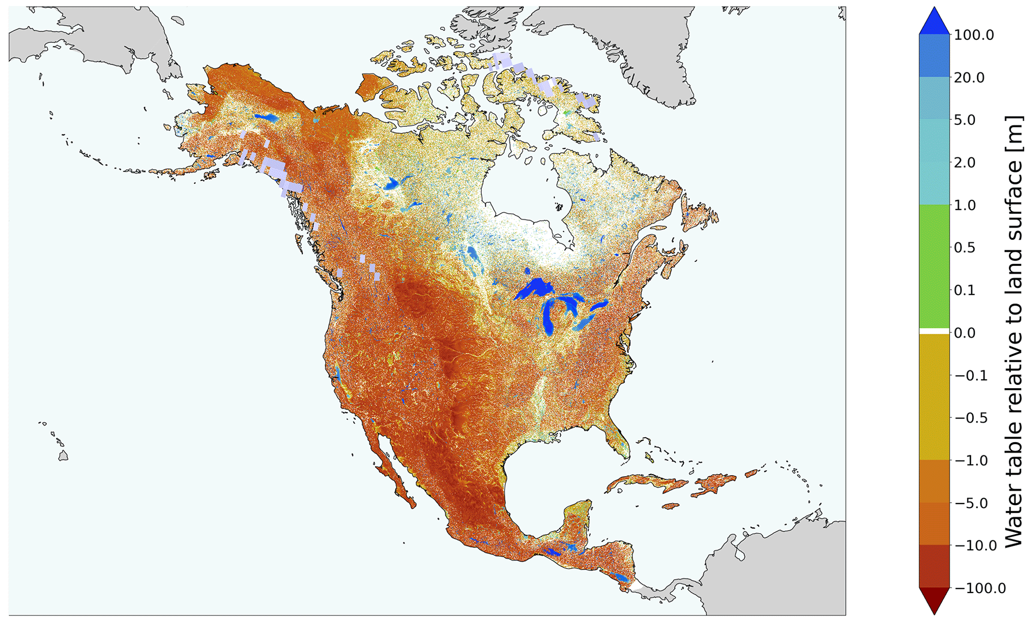
Figure 3 Simulated climate-driven water table for present-day North America. This simulation is representative of the climate-driven steady-state water table for the time period from ∼ 1958–2018, following a 20 000-year spin-up to a steady state. Positive values indicate lake depths, and negative values indicate the depth of groundwater tables beneath the land surface. The basemap includes both ocean (pale cyan) and land (grey). Continental ice thickness from ICE-6G (Peltier et al., 2015) varies from thin (blue-grey) to thick (white), with most modern ice being thin.

To reach a steady state, we ran this simulation for over 20 000 years. This duration is significantly longer than the global median groundwater response time of 5727 years noted by Cuthbert et al. (2019a); furthermore, Cuthbert et al. (2019a) report a groundwater response time of 1238 years when excluding hyper-arid regions and note that approximately 25 % of the Earth's land surface responds within 100 years. To confirm whether our simulation had reached a reasonable degree of equilibration, we computed e-folding response times for the equilibration of our simulated water table for every cell in the domain. We found that the median e-folding response time for our present-day WTM simulation was 2792 years. Our 20 000-year-long simulation was more than 7 times the length of this e-folding response time, meaning that we expected the water table to be more than 99.9 % equilibrated.

6.1.1 Model validation: comparison with observations

We compare our simulation results to water-table observational data covering 2.87 % of the cells within our North American domain. This coverage comprises 21 % groundwater wells, 25 % lake cells, and 54 % wetlands. Groundwater-table data come from an extensive archive of water-table observations gathered by Fan et al. (2013). After removing readings with negative water-table depths, water-table depths greater than the listed maximum well depth for the dataset, and “nodata” values provided for either the water table or the topography, more than 900 000 data points remained. We then averaged the values in cases with multiple data points per grid cell, leaving over 500 000 cells containing groundwater observations. Lake data (Kourzeneva et al., 2012) consisted of spatially distributed bathymetry measurements for large lakes and mean depths for thousands of smaller lakes, including a default value of 10 m where depth was unknown. In some cases, the extents of those lakes represented by only mean depth from the Kourzeneva et al. (2012) dataset exceeded those represented by flat surfaces in the GEBCO Bathymetric Compilation Group (2020) topographic dataset, causing spurious results in the data–model comparison. To prevent this, we reduced the size of all lakes by five 30 arcsec cells. Although some good data were removed through this process, it also removed the problematic data and allowed for a more reliable data–model comparison. Finally, we processed the wetland data (Zhang et al., 2023a) to remove the “permanent water” (i.e. lake) class since lakes are better represented by the Kourzeneva et al. (2012) dataset. Because this dataset does not include water-table depths, we assumed that wetlands had a relative water-table elevation equal to 0 m – i.e. that the water table was at the land surface. The Zhang et al. (2023a) dataset has a spatial resolution of 30 m; we defined each of our 30 arcsec cells as a wetland if it contained more than 50 % wetlands based on the finer-resolution data. The locations of cells containing each type of observation are given in Fig. F1.

A comparison of the distributions of water-table depths in both the simulation and the observations (Fig. 4) shows a strong match across most depths. Because the wetland data cover a larger spatial area than the groundwater and lake data, they represent a high proportion of the data in these histograms. The histograms also emphasise several issues with the observed dataset: (1) the Kourzeneva et al. (2012) lake dataset provides only mean depths for the majority of the lakes included, and, in addition, the lake size had to be reduced to avoid spurious data where the lake extents did not spatially match with the lakes in the GEBCO Bathymetric Compilation Group (2020) topography. As a result, there are few very shallow-water lake cells in the observations compared to the simulation. (2) Although we assume that wetland cells have water tables exactly at the land surface, they may, in reality, lie above or below it. Our assumption that wetlands have a water table corresponding to the land surface results in a peak in the data at 0 m, while near-zero values remain undersampled. (3) Groundwater wells might not sample the full range of actual groundwater depths, especially in locations with very shallow or very deep water tables (Fan et al., 2013). (4) Groundwater pumping may occur at or near some wells, depressing the observed water table. These issues may account for a substantial amount of the discrepancy seen between the simulation and observations. Improvements in observed data in the future will enable us to better test simulated results. Improvements in model inputs (such as input gridded data products), including observations and simulations of topography and climate, should also increase the accuracy of WTM results in the future.

Scatter plots show some variation between simulated and observed water tables on a cell-by-cell basis (Fig. 5), though it is notable that many simulated cells match the observations. The many potential reasons for discrepancies include seasonal variations in observed data, the water table not being in a steady state in the real world, and differences in the water table and topography within the 30 arcsec cell size. On the other hand, there is very close agreement between the modelled and observed hydraulic head, indicating that the hydraulic head is likely dominated by the topographic signal. It is notable that data–model matches are significantly more correlated in lake and wetland regions than in groundwater. This highlights an important difference between the data types used in the observations of each of these: lake and wetland data represent the water depth across the entire area of a cell, while groundwater well data represent the depth at a single point within the cell. Since the topography within a 30 arcsec cell may be variable, the depth to groundwater also varies; our model aims to provide a mean value for the cell.

A few discrepancies in the comparison of water-table depths in Fig. 5a can be explained by an inadequacy in the input data used for the WTM in this simulation: our data for the open-water evaporation layer did not account for lake ice reducing evaporation in northern-latitude lakes. As a result, some lakes in northern North America are simulated with water that is significantly shallower than in reality. This causes the vertical line seen at a simulation value of 0, as well as the diagonal lines extending out from it. These issues could likely be resolved, and more accurate lake depths acquired, by including lake ice in the input data.

It should be noted that our results are highly dependent on the input data used. Uncertainty in the input data will, as with all models, propagate into the results. We attempt to reduce any issues with short-term weather variability by averaging the climate data over multiple years, as discussed in Appendix E. As such, the validation in this section is relevant only for the particular datasets used in this simulation.

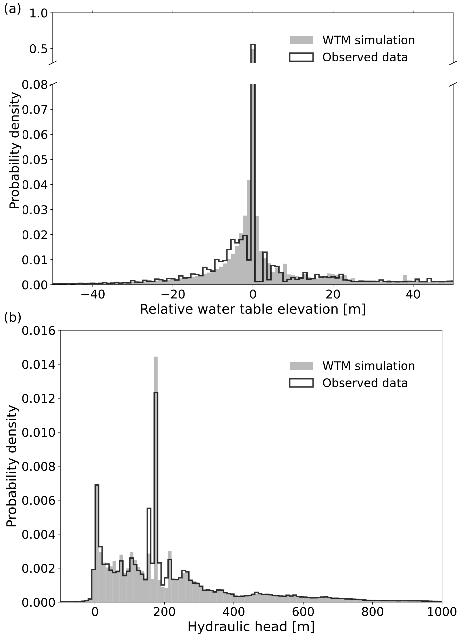
Figure 4 Simulated versus observed present-day climate-driven water tables for North America. (a) Relative water-table elevation. (b) Hydraulic head. Observations include lake, wetland, and groundwater well data from Kourzeneva et al. (2012), Zhang et al. (2023a), and Fan et al. (2013), respectively. The dates represented by these data span the period from 1927 (for some of the wells) to 2020. A small proportion of both observed and simulated relative water-table elevations and heads lie outside the x-axis limits.

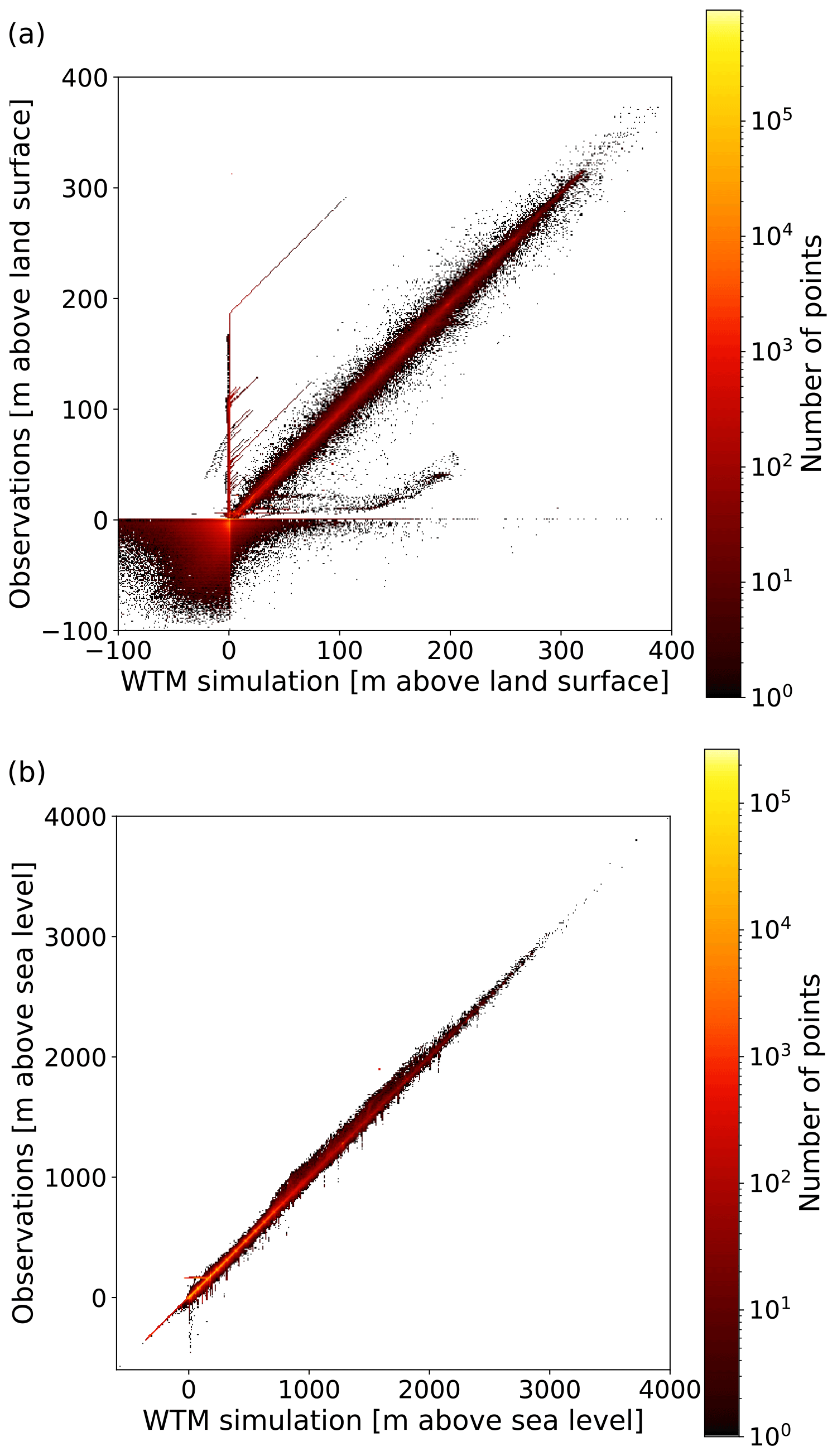
Figure 5 Observations vs. present-day climate-driven simulation results from the WTM. (a) Relative water-table elevation. (b) Hydraulic head. Observations include lake, wetland, and groundwater well data from Kourzeneva et al. (2012), Zhang et al. (2023a), and Fan et al. (2013), respectively. The dates represented by these data span the period from 1927 (for some of the wells) to 2020. These comparisons include only model cells that contain observations.

6.1.2 Model benchmarking: comparison with other simulations

Here, we compare results from the WTM's present-day simulation to results from two steady-state simulations of the present-day climate-driven groundwater table for North America – the Fan et al. (2013) model and the Reinecke et al. (2019b) model (G³M). We choose these models as comparative datasets because they are both prominent models that, like ours, aim to improve large-scale representations of the water table. They both provide continental-scale simulations of the groundwater table, with an approach to groundwater movement that has similarities to our own. The key differences include our inclusion of dynamic lake surfaces and the capability of our model to produce transient results.

The Fan et al. (2013) 30 arcsec resolution simulation did not include lake water and instead assumed that all water above the land surface would either evaporate or run off. A comparison with the WTM is shown in Fig. 6a and b. G³M (Reinecke et al., 2019b), like the WTM, focuses on simplicity and drives groundwater flow using hydraulic head. However, the 5 arcmin resolution G³M simulation treats surface water as a static boundary condition, with prescribed proportions of both lake and wetland extents in each model cell. Positive water-table elevation values in the G³M outputs do not represent actual lake depths, and surface water may be exported to the static lake and wetland classes (not included within the reported results). A comparison with the WTM simulation is shown in Fig. 6c and d.

The inclusion of dynamic lakes in the WTM simulation accounts for a large proportion of the difference in the relative water-table elevation distribution between this simulation and the other two. We note that, due to the inclusion of lake surfaces in our work, we also expect water tables in areas surrounding lakes to be higher than those simulated by Fan et al. (2013) or G³M (Reinecke et al., 2019b), due to the increased hydraulic head in these regions. As expected, the WTM shows positive relative water-table elevations (indicative of lake depths) and a larger proportion of cells in the −0.5 to 0.5 m range (incorporating shallow groundwater) than either of the other simulations. The Fan et al. (2013) and G³M (Reinecke et al., 2019b) simulations instead exhibit greater proportions of cells in slightly deeper groundwater categories. The significantly lower proportion of cells in the −0.5 to 0.5 m range in the G³M simulation may be a result of the export of water to their wetland and lake classes, which were not provided in their results. Head values, which are largely dominated by topography, align well across the simulations. The WTM output contains fewer low head values than either of the other simulations. This may result from the inclusion of lake surfaces in the WTM, which increases the average head.

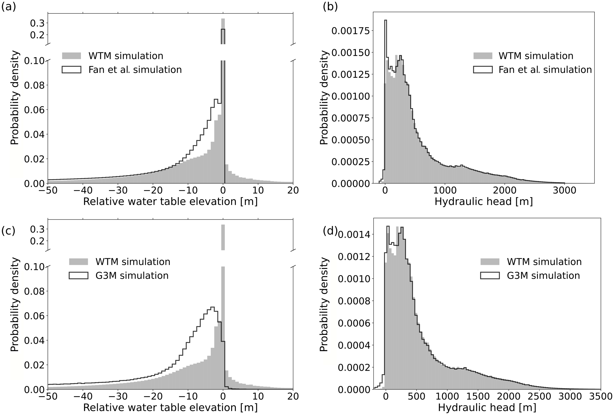
Figure 6 Comparing the WTM-computed present-day results against (a, b) the Fan et al. (2013) simulation results and (c, d) the G³M simulation results. These histograms compare the probability density functions of relative water-table elevation (a, c) and hydraulic head values (b, d), with the WTM simulations indicated by grey regions and the other simulations represented by black lines. Note the y-axis break in panels (a) and (c), which accommodates the peak in near-zero values.

6.2 North America steady-state simulation: Last Glacial Maximum

To demonstrate the ability of the WTM to simulate the depth to the water table at different times under different geographic and climatic conditions, we used the WTM to simulate the steady-state water table at a 30 arcsec spatial resolution for the North American continent at 21 ka (21 000 calendar years before present), i.e. during the Last Glacial Maximum (LGM) (Fig. 7; for input data, see Appendix E). This proof-of-concept simulation shows how the WTM can be used to simulate the water table at different times throughout the Earth's history. During the LGM, the world was on the verge of experiencing thousands of years of dramatic sea-level rise, ice retreat, and climate change. Additionally, lower sea levels, greater ice extent, and different climate conditions at that time all contributed to a water table that differed from today's.

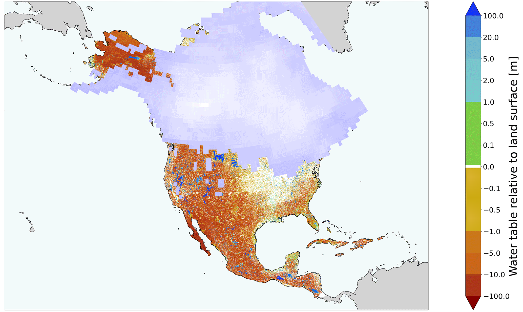
Figure 7 Simulated water table for North America during the LGM (21 ka). This simulation is representative of the climate-driven steady-state water table for 21 000 calendar years before the present, following a 20 000-year spin-up to reach a steady state. Positive values indicate lake depths, and negative values indicate the depth of groundwater tables beneath the land surface. The basemap includes both ocean (pale cyan) and land (grey). Continental ice thickness from ICE-6G (Peltier et al., 2015) varies from thin (blue-grey) to thick (white).

From 30 to 20 ka, sea levels and ice extent changed relatively little compared to the deglaciation that followed (Lambeck et al., 2014). Therefore, although it is still unlikely that the water table was fully in a steady state, it is a more reasonable assumption with respect to the LGM than for any subsequent time period until the late Holocene. To reach a steady state, we ran the simulation for over 20 000 years, which, again, is significantly longer than the present-day global median groundwater response time of 5727 years (Cuthbert et al., 2019a). As before, we evaluated the e-folding response time within our LGM simulation of North America and found it to be 4559 years; we therefore expected our water table to be more than 98 % equilibrated. In this simulation, we used a palaeotopography that accounts for glacial isostatic adjustment (GIA) and is forced by past ice sheets (Peltier et al., 2015) and outputs from palaeoclimate general circulation models (GCMs) (He, 2011).

In comparison with the present-day climate-driven water table shown in Fig. 3, the LGM water table (Fig. 7) is noticeably higher in the eastern portions of the continent, and there is significantly more lake water visible in the west and south (Fig. 8a). Note also the larger ice extent and lower sea level during the LGM. Broadly speaking, the changes in water-table depth match the changes in P−ET (precipitation minus evapotranspiration) (Fig. 8b). Most regions with increased levels of P−ET experienced higher water tables, and vice versa. The ice sheets and associated glacial isostatic adjustment also played a role: ice thickness provided a pressure head that drove both surface-water and groundwater flow, and ice melt both added water and altered the topography, which here also includes ice-sheet contributions to driving flow (see the LGM ice extent in Figs. 7 and 8). GIA primarily caused land uplift from the LGM to the present day, thereby increasing the elevation head. The higher head values in northern North America during the LGM (from overlying ice) may have played a role in moving groundwater further south – consistent with the model-based findings of Lemieux et al. (2008) – resulting in higher water tables to the south of the ice-sheet margin at that time.

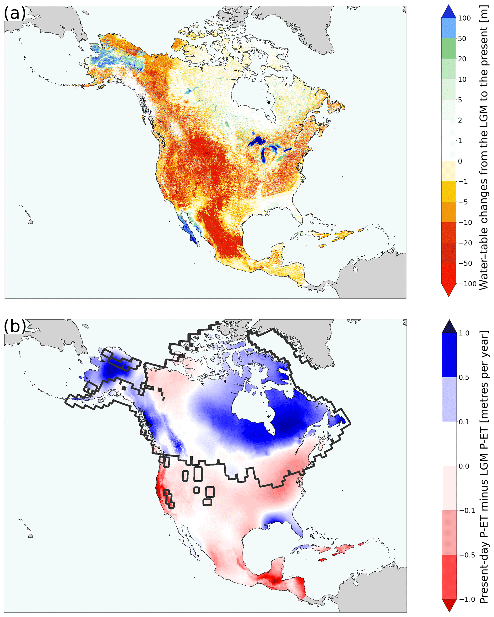
Figure 8 The present-day climate-driven water table minus the LGM water table (a). The Great Lakes filled with water following their deglaciation. A warmer and drier climate (b) reduces terrestrial water storage more broadly, especially in the west. The solid dark-grey line in panel (b) represents the ice extent during the LGM.

In total, water tables during the LGM were higher than those of the present day (Fig. 3), with the difference between the two simulations amounting to 14.98 cm of sea-level equivalent (SLE) (approximately 54.2×10¹⁵ L of water). Over this time period, lake storage increased by 5.77 cm SLE – predominantly as a result of the Great Lakes becoming deglaciated. Despite this change in lake volume, we can observe, as shown in Fig. 7, that many now-vanished lakes existed, especially along the ice margin and in currently arid regions. Meanwhile, groundwater storage decreased by 20.75 cm SLE from the LGM to the present day. This change appears to have been largely driven by changes in climate. Note that both simulations assumed a steady-state water table and that this result may be different when simulating a transient change in the water table.

7 Conclusions

Long-term changes in the water table impact the entire hydrologic cycle, including sea levels and climate. Despite this, little is known about changes in the water table over timescales longer than decades. The WTM provides a new capability for computing long-term, continental-scale changes in water tables and terrestrial water storage, including both the groundwater table and dynamically changing lake surfaces. The WTM's simple input requirements mean that it can simulate water tables from the distant past or future as the climate continues to change, and the model is capable of both steady-state and transient simulations. Initial proof-of-concept model runs have indicated that water storage across a continent can change by several centimetres of sea-level equivalent under natural climate change conditions and that changes in water-table depth broadly follow the patterns of changing levels of P−ET.

Appendix A: Model inputs, logical flow, and outputs

A1 Data input requirements

The WTM requires the following 2D, horizontally distributed input arrays for all steady-state or transient model runs:

• Topography. This refers to land elevation above sea level (metres). At the user's discretion, this can be modified to include overlying ice.

• Slope. This refers to the topographic slope, which should be based on the input topography data (unitless).

• Ocean mask. A binary mask is used, with values of 1 indicating land cells and values of 0 indicating ocean cells.

• Climatic water input. Precipitation, along with (if applicable) ice melt or any other water entering the system, serves as the climatic water input (metres per year).

• Evapotranspiration. Evapotranspiration refers to the actual ET occurring over land (metres per year).

• Open-water evaporation. This refers to the evaporation (potential ET) that occurs when there is open surface water, e.g. a lake (Appendix D) (metres per year).

• Winter temperature. This concerns temperatures during the months of December, January, and February in the Northern Hemisphere and during the months of June, July, and August in the Southern Hemisphere (degrees Celsius).

• Shallow-subsurface hydraulic conductivity – horizontal. This refers to horizontal hydraulic conductivity (K_1.5 in Eq. 5), representative of near-surface conditions (metres per second).

• Porosity. This refers to shallow-subsurface porosity (ϕ in Eq. 9) (unitless).

For transient model runs, separate input arrays are required for the start and end times for the topography, slope, climatic water input, evapotranspiration, open-water evaporation, winter temperature, and runoff ratio (optional). The values of these arrays change linearly over time, from the start to the end values. In addition, transient model runs require a starting relative water-table elevation.

In some cases, the following optional input data may be used:

• Starting relative water-table elevation. This input, required for transient model runs, is also provided as an option for steady-state runs. It allows users to reach a steady state more rapidly if there is some initial knowledge about the water table, or it allows users to break the model run up into several shorter runs by using previous outputs as input for this array. The relative water-table elevation (z_wr) is defined as the water-table elevation minus the elevation of the land surface (metres). Positive values indicate the presence of a lake, while negative values indicate a groundwater table. If this input is not supplied, z_wr will be initialised at a value of 0 (corresponding to the land surface), and the model must first be run to a steady state before any transient model runs can be performed. The simulations included in this paper initialised the water table at a value of 0.

• Runoff ratio. (This is optional, i.e. at the user's discretion.) If provided, the difference between precipitation and evapotranspiration (P−ET) will be split into groundwater recharge and overland runoff using this array of runoff ratios. If not provided, this difference (P−ET) is used entirely as recharge and is added directly to the groundwater table in the cell where it falls.

• Shallow-subsurface hydraulic conductivity – vertical. (This is optional, i.e. only required if the infiltration option is enabled – see Sect. 4.2.1.) Vertical hydraulic conductivity representative of near-surface conditions (metres per second) is used. If this input is not provided, the infiltration option must be disabled.

A2 Logical flow

The logical flow of the WTM is shown in Fig. A1. Model inputs, as described in Appendix A1, are provided, and the depression hierarchy for the given topography is calculated. In transient runs, the input files are updated over time as conditions change; the depression hierarchy is recalculated as the topography changes. The model then adds the appropriate recharge to the water table and (1) moves groundwater, (2) moves surface water, and (3) calculates the climatic water balance (precipitation minus evapotranspiration, plus ice melt or any other water inputs/outputs) for the next time step. The evapotranspiration field is updated to use the Penman equation result (Appendix D), i.e. the “open-water evaporation” input file, wherever the water table lies above the surface, and the evapotranspiration input file is used elsewhere. The model concludes after it reaches the prescribed total number of time steps. At this point, it writes the outputs to a file. Outputs are also saved at regular intervals throughout the model run.

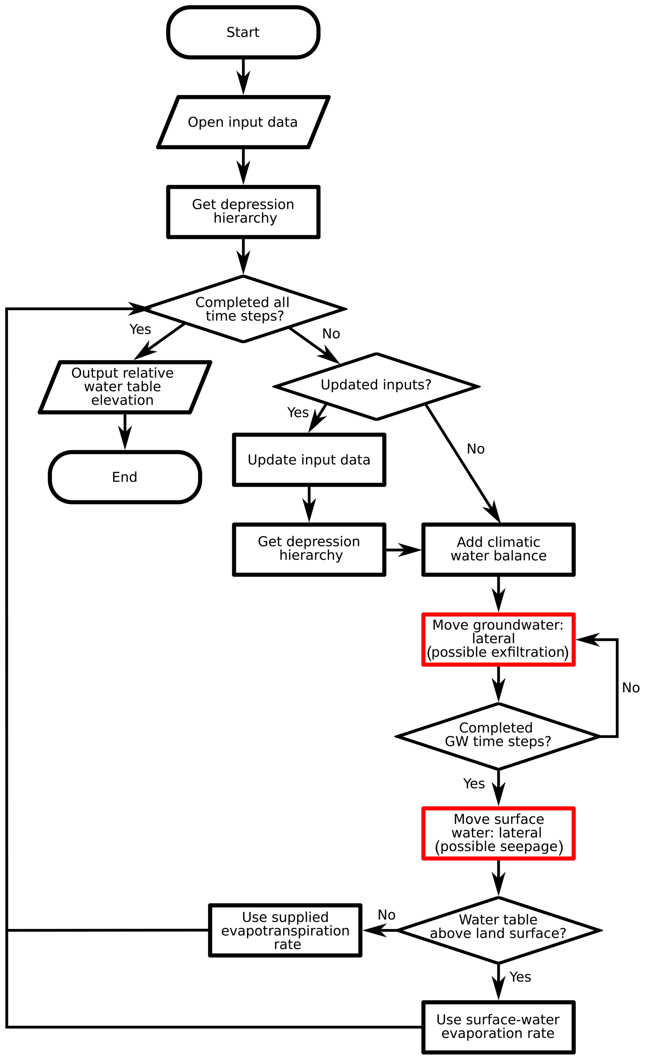
Figure A1 Steps taken by the WTM. The two red boxes indicate the components used to couple groundwater (GW) and surface water.

A3 Outputs

The WTM generates two outputs:

• the relative water-table elevation (gridded raster), saved at the end of the model run and at regular intervals throughout;

• a text file recording the number of cycles completed and the amount of water-table change occurring during each step of the simulation.

Appendix B: Solving the non-linear groundwater equation

We solve for the change in groundwater head over time using the 2D horizontal groundwater equation for saturated groundwater flow in an unconfined aquifer within a heterogeneous medium, which is assumed to be horizontally isotropic due to a lack of directional data for hydraulic conductivity (Freeze and Cherry, 1979). We invoke the Dupuit–Forchheimer theory of free-surface flow, which is based on two assumptions: (1) flow is horizontal, and (2) the hydraulic gradient is equal to the gradient of the water-table surface and does not vary with depth. The equation is as follows:

$$\begin{array}{}\text{(B1)}& {\displaystyle }{S}_{\mathrm{y}}{\displaystyle \frac{\partial h}{\partial t}}={\displaystyle \frac{\partial }{\partial x}}\left(T{\displaystyle \frac{\partial h}{\partial x}}\right)+{\displaystyle \frac{\partial }{\partial y}}\left(T{\displaystyle \frac{\partial h}{\partial y}}\right)+R,\end{array}$$

where h is the groundwater head, T is the transmissivity, t is the length of a single time interval, x and y are the two dimensions of groundwater movement, R represents recharge, and S_y is the specific yield of the aquifer (here approximated as being equal to the porosity). Note that our assumptions that the aquifer is unconfined and that groundwater flows in two dimensions allow us to use T in this formula, where T=Kh and K is the hydraulic conductivity. More information about our treatment of transmissivity is given in Sect. 3.2.

When using the Dupuit–Forchheimer approximation, discharge (Q) is defined as follows (Eq. 5.28 in Freeze and Cherry, 1979):

$$\begin{array}{}\text{(B2)}& Q=-T{\displaystyle \frac{\mathrm{\Delta }h}{\mathrm{\Delta }d}},\end{array}$$

where Δd refers to the distance in either the x (S–N) or y (W–E) direction, as appropriate.

Combining Eqs. (B2) and (B1) gives

$$\begin{array}{}\text{(B3)}& S_{\mathrm{y}}{\displaystyle \frac{\partial h}{\partial t}}=-{\displaystyle \frac{\partial Q_x}{\partial x}}-{\displaystyle \frac{\partial Q_y}{\partial y}}+R.\end{array}$$

Defining Q for each of the cardinal directions gives

$$\begin{array}{}\text{(B4)}& {\displaystyle }{Q}_{\mathrm{E}}=-T_{i+\mathrm{1}/\mathrm{2}}\left({\displaystyle \frac{h_{t(i+\mathrm{1},j)}-h_{t(i,j)}}{\mathrm{\Delta }x}}\right),\text{(B5)}& {\displaystyle }{Q}_{\mathrm{W}}=-T_{i-\mathrm{1}/\mathrm{2}}\left({\displaystyle \frac{h_{t(i,j)}-h_{t(i-\mathrm{1},j)}}{\mathrm{\Delta }x}}\right),\text{(B6)}& {\displaystyle }{Q}_{\mathrm{N}}=-T_{j+\mathrm{1}/\mathrm{2}}\left({\displaystyle \frac{h_{t(i,j+\mathrm{1})}-h_{t(i,j)}}{\mathrm{\Delta }y}}\right),\text{(B7)}& {\displaystyle }{Q}_{\mathrm{S}}=-T_{j-\mathrm{1}/\mathrm{2}}\left({\displaystyle \frac{h_{t(i,j)}-h_{t(i,j-\mathrm{1})}}{\mathrm{\Delta }y}}\right).\end{array}$$

Here, i is the cell index along the x (S–N) axis and j is the cell index along the y (W–E) axis. Note that we assess T at the cell boundaries rather than at the cell centres. We do this because mass transfer occurs across these cell boundaries, so calculating the gradients here provides more accurate directional water discharges. We indicate this cell-boundary-based calculation with the “$+\mathrm{1}/\mathrm{2}$” and “$-\mathrm{1}/\mathrm{2}$” subscripts.

Substituting these definitions of Q into Eq. (B3) and expanding the left-hand side gives

$$\begin{array}{}\text{(B8)}& \begin{array}{rl}{S}_{\mathrm{y}}{\displaystyle \frac{h_{t+\mathrm{1}(i,j)}-h_{t(i,j)}}{\mathrm{\Delta }t}}& =T_{(i+\mathrm{1}/\mathrm{2})}\left({\displaystyle \frac{h_{t(i+\mathrm{1},j)}-h_{t(i,j)}}{\mathrm{\Delta }{x}^{\mathrm{2}}}}\right)\\ & -T_{(i-\mathrm{1}/\mathrm{2})}\left({\displaystyle \frac{h_{t(i,j)}-h_{t(i-\mathrm{1},j)}}{\mathrm{\Delta }{x}^{\mathrm{2}}}}\right)\\ & +T_{(j+\mathrm{1}/\mathrm{2})}\left({\displaystyle \frac{h_{t(i,j+\mathrm{1})}-h_{t(i,j)}}{\mathrm{\Delta }{y}^{\mathrm{2}}}}\right)\\ & -T_{(j-\mathrm{1}/\mathrm{2})}\left({\displaystyle \frac{h_{t(i,j)}-h_{t(i,j-\mathrm{1})}}{\mathrm{\Delta }{y}^{\mathrm{2}}}}\right)\\ & +R.\end{array}\end{array}$$

Solving for the head at the next time step, h_t+1, gives

$$\begin{array}{}\text{(B9)}& \begin{array}{rl}{h}_{t+\mathrm{1}(i,j)}& =[T_{(i+\mathrm{1}/\mathrm{2})}\left({\displaystyle \frac{h_{t(i+\mathrm{1},j)}-h_{t(i,j)}}{\mathrm{\Delta }{x}^{\mathrm{2}}}}\right)\\ & -T_{(i-\mathrm{1}/\mathrm{2})}\left({\displaystyle \frac{h_{t(i,j)}-h_{t(i-\mathrm{1},j)}}{\mathrm{\Delta }{x}^{\mathrm{2}}}}\right)\\ & +T_{(j+\mathrm{1}/\mathrm{2})}\left({\displaystyle \frac{h_{t(i,j+\mathrm{1})}-h_{t(i,j)}}{\mathrm{\Delta }{y}^{\mathrm{2}}}}\right)\\ & -T_{(j-\mathrm{1}/\mathrm{2})}\left({\displaystyle \frac{h_{t(i,j)}-h_{t(i,j-\mathrm{1})}}{\mathrm{\Delta }{y}^{\mathrm{2}}}}\right)\\ & +R]{\displaystyle \frac{\mathrm{\Delta }t}{S_{\mathrm{y}}}}+h_{t(i,j)}.\end{array}\end{array}$$

This equation can now be broken down into the thing that we want (h_t+1) and the things that we know. We solve the equation using the PETSc SNES solver (Balay et al., 1997, 2022a, b).

Appendix C: Infiltration of surface water

C1 Transit time across a cell

To calculate the amount of infiltration that happens while water is in transit across a cell, we must consider the total time that water takes to cross the cell. The longer water remains in a cell, the more time it has to infiltrate. Water takes longer to flow across cells that are larger or have shallower slopes, as well as when the water depth – and consequently its flow velocity – is smaller.

We use Manning's equation to estimate the time taken for water to flow across a cell. This equation is expressed as

$$\begin{array}{}\text{(C1)}& u={\displaystyle \frac{\mathrm{1}}{n}}{R}_{\mathrm{h}}^{\mathrm{2}/\mathrm{3}}{S}^{\mathrm{1}/\mathrm{2}},\end{array}$$

where u is the mean (i.e. vertically averaged) velocity of the surface water moving across the cell, n is the Gauckler–Manning coefficient, R_h is the hydraulic radius, and S is the slope. By default, we set the n value in Manning's equation to 0.05 m${}^{-\mathrm{1}/\mathrm{3}}$ s. We make the assumption that the height of the water in the cell, h, is much smaller than the cell width. This allows us to simplify the hydraulic radius to be equal to h, as shown in the following:

$$\begin{array}{}\text{(C2)}& u={\displaystyle \frac{\mathrm{1}}{n}}{h}^{\mathrm{2}/\mathrm{3}}{S}^{\mathrm{1}/\mathrm{2}}.\end{array}$$

Because S and n are both constants, for convenience, we will combine them into a constant (k₀), where

$$\begin{array}{}\text{(C3)}& k_{\mathrm{0}}={\displaystyle \frac{S^{\mathrm{1}/\mathrm{2}}}{n}},\end{array}$$

so that

$$\begin{array}{}\text{(C4)}& u=k_{\mathrm{0}}{h}^{\mathrm{2}/\mathrm{3}}.\end{array}$$

The next step is to consider the infiltration rate,

$$\begin{array}{}\text{(C5)}& {\displaystyle \frac{\mathrm{d}h}{\mathrm{d}{t}_I}}=-k_{\text{sat}}.\end{array}$$

By separating the variables, integrating, and defining h=h₀ at t_I=0, we obtain

$$\begin{array}{}\text{(C6)}& h=h_{\mathrm{0}}-k_{\text{sat}}{t}_I.\end{array}$$

We substitute Eq. (C6) into Eq. (C4) and use the definition of velocity as the time derivative of position to set up the final equation in order to integrate as follows:

$$\begin{array}{}\text{(C7)}& {\displaystyle \frac{\mathrm{d}L}{\mathrm{d}t}}=k_{\mathrm{0}}{\left(h_{\mathrm{0}}-k_{\text{sat}}{t}_I\right)}^{\mathrm{2}/\mathrm{3}},\end{array}$$

where L is the displacement in an arbitrary orientation. By separating the variables and solving via a u substitution, we obtain

$$\begin{array}{}\text{(C8)}& \begin{array}{rl}L& =k_{\mathrm{0}}\underset{\mathrm{0}}{\overset{t_i}{\int }}(h_{\mathrm{0}}-k_{\text{sat}}{t}_I{)}^{\mathrm{2}/\mathrm{3}}\mathrm{d}t\\ & =-{\displaystyle \frac{\mathrm{3}}{\mathrm{5}}}{\displaystyle \frac{k_{\mathrm{0}}}{k_{\text{sat}}}}(h_{\mathrm{0}}-k_{\text{sat}}{t}_I{)}^{\mathrm{5}/\mathrm{3}}+c,\end{array}\end{array}$$

where c is the constant of integration. Defining L as 0 when t_I=0 (i.e. with the clock starting when the water first touches the cell margin), we obtain

$$\begin{array}{}\text{(C9)}& c={\displaystyle \frac{\mathrm{3}}{\mathrm{5}}}{\displaystyle \frac{k_{\mathrm{0}}}{k_{\text{sat}}}}{h}_{\mathrm{0}}^{\mathrm{5}/\mathrm{3}}.\end{array}$$

This means the distance crossed by the water is given as

$$\begin{array}{}\text{(C10)}& L={\displaystyle \frac{\mathrm{3}}{\mathrm{5}}}{\displaystyle \frac{k_{\mathrm{0}}}{k_{\text{sat}}}}\left(h_{\mathrm{0}}^{\mathrm{5}/\mathrm{3}}-(h_{\mathrm{0}}-k_{\text{sat}}{t}_I{)}^{\mathrm{5}/\mathrm{3}}\right).\end{array}$$

We rearrange this expression to find the amount of time that this transit takes because this is the amount of time that the water has to infiltrate into the ground in the cell. Solving for the transit time and substituting S and n back into the equation gives

$$\begin{array}{}\text{(C11)}& t_I=\left[h_{\mathrm{0}}-{\left(h_{\mathrm{0}}^{\mathrm{5}/\mathrm{3}}-{\displaystyle \frac{\mathrm{5}}{\mathrm{3}}}{\displaystyle \frac{n}{S^{\mathrm{1}/\mathrm{2}}}}{k}_{\text{sat}}\mathrm{\Delta }L\right)}^{\mathrm{3}/\mathrm{5}}\right]/k_{\text{sat}}.\end{array}$$

In the WTM, we limit the topographic slope, S, to a minimum value of 10⁻⁶ to allow for movement over flat cells in the DEM. We calculate L based on the direction of travel between the two cells (north–south, east–west, or diagonally) and the latitude of the cells.

C2 Infiltration

We now understand the time (t_I) it takes for water to cross a cell as a function of the distance travelled by the water from cell to cell (L), slope (S), and flow depth (h). When water flows across a cell that is not already groundwater-saturated, the flow depth decreases as it crosses the cell due to infiltration. This occurs at a rate governed by the saturated vertical hydraulic conductivity (k_sat); for simplicity, we do not consider transient wetting and drying effects in the unsaturated zone. Some water will undergo infiltration, and some will continue to flow downslope as infiltration-excess overland flow (Horton and Htrata, 1955). When water crosses a cell that is already fully saturated (i.e. when the groundwater table is at the land surface), no infiltration is possible, and saturation-excess overland flow (Dunne and Black, 1970) will occur.

There are two possible solutions for the potential total amount of water infiltration (I_pot), given by

$$\begin{array}{}\text{(C12)}& I_{\text{pot}}=\left\{\begin{array}{ll}{h}_{\mathrm{0}}& \text{if }{h}_{\mathrm{0}}^{\mathrm{5}/\mathrm{3}}\le \frac{\mathrm{5}}{\mathrm{3}}\frac{n}{S^{\mathrm{1}/\mathrm{2}}}{k}_{\text{sat}}\mathrm{\Delta }L,\\ k_{\text{sat}}{t}_I& \text{otherwise}.\end{array}\right.\end{array}$$

In the first case, the entire column of water that enters the cell may undergo infiltration before it crosses the cell. For the “=” subcase, the travel time corresponds precisely to the infiltration time; for the “<” subcase, the solution to Eq. (C11) becomes undefined because all the water undergoes infiltration before completing its crossing. In the second case, the potential infiltration simply equals the saturated hydraulic conductivity multiplied by the amount of time that this water can infiltrate before it crosses the cell; remaining water continues to flow into the next cell.

Converting I_pot to the actual amount of infiltration that occurs, I, requires consideration of the space available to accommodate infiltration water. Combining Eq. (C12) with the amount of groundwater space available in the cell – given by −ϕz_wr, where ϕ is the subsurface porosity (assumed constant with depth) and z_wr is the relative water-table elevation – provides the general solution, expressed as

$$\begin{array}{}\text{(C13)}& I=min\left(-\mathit{\varphi }{z}_{\mathrm{wr}},I_{\mathrm{pot}}\right).\end{array}$$

This amount of infiltrated water is then subtracted from the flow depth, h. If h>0 as the water exits the cell, then the water continues onwards to the next downslope cell.

Appendix D: Open-water evaporation

We calculate open-water evaporation by solving and applying the Penman equation (Dingman, 1994) together with the Charnock (1955) expression for the roughness length over open water as a function of wind-induced waves. This evaporation rate overrides the input evapotranspiration rate whenever the water table crops out above the ground surface, forming an exposed waterbody (Fig. A1). The effects of ice cover are not considered.

The Penman (1948) equation combines radiative, sensible, and latent heat transfer to solve for evaporation. Though this equation is well established (Finch and Calver, 2008; Valiantzas, 2006; Vörösmarty et al., 1998; Zotarelli and Dukes, 2010), we choose to include a brief derivation of the Penman equation due to (1) the central role evaporation plays in our study; (2) the fact that most derivations centre on the Penman–Monteith equation (Monteith, 1965), which involves plant transpiration that is not relevant to our application to lakes; and (3) our inclusion of a wind-speed-determined roughness length for modulating wind-driven turbulent energy transfers, which seems reasonable to include but did not appear in our review of the literature. Here, we use variable nomenclature that is more common to thermodynamics than to hydrology.

D1 Penman equation (general form)

The Penman equation relates the evaporation rate (E), which corresponds to latent heat flux, to net radiation flux (R_n – incoming and outgoing shortwave and longwave radiation) and sensible heat flux due to turbulent atmospheric heat transfer (Q_H,s – where the subscript “H” indicates enthalpy and the subscript “s” indicates that this enthalpy is sensible). Accordingly, E is expressed as

$$\begin{array}{}\text{(D1)}& E={\displaystyle \frac{R_{\mathrm{n}}-Q_{H,\mathrm{s}}}{{\mathit{\rho }}_{\mathrm{w}}\mathrm{\Delta }{H}_{\text{vap}}}}.\end{array}$$

Here, ρ_w is water density and ΔH_vap is the latent heat of vaporisation of water. These denominator terms convert the energy fluxes (W m⁻²) into evaporation (m s⁻¹).

D2 Input data products

Inputs for our solution come from the TerraClimate and GEBCO_2020 datasets. TerraClimate (Abatzoglou et al., 2018) comprises monthly gridded data products at a 2.5 arcmin resolution (∼ 5 km from N–S) for the following:

• incoming solar (shortwave) radiation

• monthly averaged minimum and maximum daily temperatures

• wind speed

• vapour pressure.

GEBCO_2020 (GEBCO Bathymetric Compilation Group, 2020) is a global gridded topographic and bathymetric dataset with a 15 arcsec resolution (∼ 0.5 km from N–S). We resampled this dataset to 2.5 arcmin to align with the resolution of TerraClimate.

D3 Net radiation

In the field, acquiring net radiation requires paired upward- and downward-facing pyranometers and pyrgeometers to measure incoming and outgoing shortwave and longwave radiation. Here, we use a combination of calculations and remotely sensed data products to assemble a solar-radiation data product at an appropriate resolution for our continental-scale modelling example.

TerraClimate (Abatzoglou et al., 2018) provides the incoming shortwave radiation flux, R_in,s. The outgoing shortwave radiation is equal to the incoming radiation multiplied by the surface albedo, α. Therefore, the net shortwave radiation, R_n,s, is given by

$$\begin{array}{}\text{(D2)}& R_{\mathrm{n},\mathrm{s}}=(\mathrm{1}-\mathit{\alpha })R_{\text{in},\mathrm{s}}.\end{array}$$

We use α=0.06 as the characteristic value for open water.

We lack data on net longwave radiation, R_n,l, but know that (1) the outgoing longwave flux is proportional to surface temperature using the Stefan–Boltzmann law and (2) that incoming longwave radiation is related to greenhouse gases in the atmosphere that absorb and re-emit this outgoing radiation. We therefore follow and modify the approach taken by Zotarelli and Dukes (2010) in both approximating the surface temperature with the maximum and minimum air temperature values and using vapour pressure and cloudiness to estimate the impact of greenhouse gases on longwave absorption and re-radiation, as shown in the following:

$$\begin{array}{}\text{(D3)}& R_{\mathrm{n},\mathrm{l}}=\mathit{\sigma }{\displaystyle \frac{T_{\text{max}}^{\mathrm{4}}+T_{\text{min}}^{\mathrm{4}}}{\mathrm{2}}}\left(\mathrm{0.34}-\mathrm{0.00014}{e}_{\mathrm{a}}^{\mathrm{1}/\mathrm{2}}\right)\mathcal{C}.\end{array}$$

Here, σ is the Stefan–Boltzmann constant, T represents temperature (expressed in kelvin), e_a is the near-surface atmospheric vapour pressure, and 𝒞 is what we choose to call the “cloud function”.

We can estimate the value of the cloud function using the difference between the clear-sky solar radiation, $R_{\text{in},\mathrm{s},\text{CS}}$, and the solar radiation received at the land surface, R_in,s. To compute the clear-sky solar radiation, we first compute the top-of-atmosphere (i.e. extraterrestrial) solar radiation ($R_{\text{in},\mathrm{s},\text{TOA}}$); see sunpos.py in Wickert (2020). We then modify it based on the elevation (Zotarelli and Dukes, 2010), which determines the atmospheric thickness above a given location as follows:

$$\begin{array}{}\text{(D4)}& R_{\text{in},\mathrm{s},\text{CS}}=\left(\mathrm{0.75}+\mathrm{2}\times {\mathrm{10}}^{-\mathrm{5}}z\right)R_{\text{in},\mathrm{s},\text{TOA}},\end{array}$$

where z, as in the main text, is the surface elevation in metres.

This method works only where sufficient incoming solar radiation exists to produce a meaningful difference between $R_{\text{in},\mathrm{s},\text{TOA}}$ and R_in,s. Based on our tests, a reasonable cutoff value for incoming solar radiation is 15 W m⁻².

$$\begin{array}{}\text{(D5)}& \mathcal{C}=\left\{\begin{array}{ll}\mathrm{1.35}\frac{R_{\text{in},\mathrm{s}}}{R_{\text{in},s,\text{TOA}}}-\mathrm{0.35}& \text{if }{R}_{\text{in},\mathrm{s},\text{TOA}}\ge \mathrm{15},\\ {\stackrel{\mathrm{‾}}{\left[\mathrm{1.35}\frac{R_{\text{in},\mathrm{s}}}{R_{\text{in},\mathrm{s},\text{TOA}}}-\mathrm{0.35}\right]}}_{\text{15–20}}& \text{otherwise},\end{array}\right.\end{array}$$

where the lower term represents the average of the upper term when $\mathrm{15}<R_{\text{in},\mathrm{s},\text{TOA}}<\mathrm{20}$. This is an obvious kludge for the sake of generating proof-of-concept model outputs, and it generates a reasonable but inaccurate cloud-function value for the polar regions.

The final step is straightforward. Net radiation flux is simply the sum of the net shortwave and longwave fluxes:

$$\begin{array}{}\text{(D6)}& R_{\mathrm{n}}=R_{\mathrm{n},\mathrm{s}}+R_{\mathrm{n},\mathrm{l}}.\end{array}$$

D4 Sensible heat flux

Deriving the Penman equation for sensible heat flux, Q_H,s, results in the following (Dingman, 1994):

$$\begin{array}{}\text{(D7)}& Q_{H,\mathrm{s}}={\displaystyle \frac{K_{\mathrm{H}}u}{{\mathrm{\Delta }}_{\mathrm{P},\mathrm{T}}}}\left[{\displaystyle \frac{E}{K_{\mathrm{E}}u}}-\left(e_{\text{sat}}-e_{\mathrm{a}}\right)\right].\end{array}$$

Here, K_H and K_E are coefficients of turbulent conductance (kg m s⁻¹ K⁻¹) for sensible heat and water vapour (i.e. latent heat), respectively. Moreover, u represents wind speed, which is conventionally measured 2 m above the surface. Δ_P,T is the slope of the liquid-to-vapour phase transition of water at air temperature (T_a), which likewise is measured 2 m above the surface. Similarly, e_sat is the saturation water vapour pressure at T_a, while e_a is the actual water vapour pressure.

The turbulent-conductance coefficients, K_H and K_E, are defined based on the ratios of heat (K_H) and water vapour (K_E) transfer to momentum transfer (Dingman, 1994):

$$\begin{array}{}\text{(D8)}& {\displaystyle }{K}_{\mathrm{H}}={\displaystyle \frac{D_{\mathrm{H}}}{D_{\mathrm{M}}}}{c}_p{\mathit{\rho }}_{\mathrm{a}}{\left({\displaystyle \frac{u_{*}}{u}}\right)}^{\mathrm{2}},\text{(D9)}& {\displaystyle }{K}_{\mathrm{E}}={\displaystyle \frac{D_{\text{WV}}}{D_{\mathrm{M}}}}{\displaystyle \frac{\mathrm{\Delta }{\mathit{\rho }}_{\mathrm{a}}}{P{\mathit{\rho }}_{\mathrm{w}}}}{\displaystyle \frac{R_{\mathrm{a}}}{R_{\mathrm{v}}}}{\left({\displaystyle \frac{u_{*}}{u}}\right)}^{\mathrm{2}}.\end{array}$$

Here, D_H represents thermal diffusivity in air, D_M is the diffusivity of momentum, and D_WV is the diffusivity of water vapour. For a stable atmosphere, which we assume, the same turbulent eddies result in the transfer of heat, momentum, and water vapour. Therefore, $D_{\mathrm{H}}/D_{\mathrm{M}}=D_{\mathrm{WV}}/D_{\mathrm{M}}=\mathrm{1}$, simplifying Eqs. (D8) and (D9) to the following:

$$\begin{array}{}\text{(D10)}& {\displaystyle }{K}_{\mathrm{H}}=c_p{\mathit{\rho }}_{\mathrm{a}}{\left({\displaystyle \frac{u_{*}}{u}}\right)}^{\mathrm{2}},\text{(D11)}& {\displaystyle }{K}_{\mathrm{E}}={\displaystyle \frac{{\mathit{\rho }}_{\mathrm{a}}}{P{\mathit{\rho }}_{\mathrm{w}}}}{\displaystyle \frac{R_{\mathrm{a}}}{R_{\mathrm{v}}}}{\left({\displaystyle \frac{u_{*}}{u}}\right)}^{\mathrm{2}}.\end{array}$$

We restate the variable definitions from the main text for convenience: c_p is the specific heat capacity of air at constant pressure, ρ_a represents air density, u_* represents wind shear velocity, u is the measured wind velocity (typically at 2 m elevation above the surface), ρ_w represents water density, P represents atmospheric pressure, and $R_{\mathrm{a}}/R_{\mathrm{v}}=\mathrm{0.622}$ is the ratio of the gas constants of air and water vapour.

D5 Full Penman equation

The process of combining Eqs. (D1) and (D7) and solving for evaporation results in the common full form of the Penman equation (see Dingman, 1994), given by

$$\begin{array}{}\text{(D12)}& E={\displaystyle \frac{\left[R_{\mathrm{n}}+\left(\frac{K_{\mathrm{H}}u}{{\mathrm{\Delta }}_{\mathrm{P},\mathrm{T}}}\right)\left(e_{\text{sat}}-e_{\mathrm{a}}\right)\right]}{\left[{\mathit{\rho }}_{\mathrm{w}}\mathrm{\Delta }{H}_{\text{vap}}+\left(\frac{K_{\mathrm{H}}}{K_{\mathrm{E}}}\frac{\mathrm{1}}{{\mathrm{\Delta }}_{\mathrm{P},\mathrm{T}}}\right)\right]}}.\end{array}$$

Substituting in the definitions of coefficients K_H and K_E, we obtain Eq. (E1).

D6 Variable water surface roughness

The u_* term in the diffusivity of momentum, D_M, can be evaluated by solving for the boundary-layer velocity profile, given by the logarithmic “law of the wall”, in which

$$\begin{array}{}\text{(D13)}& u\left(z\right)={\displaystyle \frac{u_{*}}{\mathit{\kappa }}}\ln \left({\displaystyle \frac{z_{\mathit{\alpha }}}{z_{\mathrm{0}}}}\right).\end{array}$$

Here, κ=0.407 is the von Kármán constant, z_α is the height of the air above the land surface, and z₀ is the surface roughness length. It is then possible to solve for u_* by knowing the wind velocity (u) at a known elevation (z_α=z₁), which is typically 2 m above the surface, and the surface roughness length scale.

When wind flows over open water, it generates waves, thereby making the roughness length itself a function of wind speed. This makes Eq. (D13) non-linear, thereby adding a layer of complexity not included in models of overland evaporation.

To address this problem, we first turn to Charnock (1955), who found a quadratic relationship between wave-generated z₀ and u_*. Hersbach (2011) expanded this work and defined z₀ over a broader range of conditions by showing that it depends on kinematic viscosity, ν, in light winds and on a shear-velocity-squared (Charnock, 1955) relationship in strong winds. Accordingly, z₀ is given by

$$\begin{array}{}\text{(D14)}& z_{\mathrm{0}}=K_{\mathit{\nu }}{\displaystyle \frac{\mathit{\nu }}{u_{*}}}+K_{\text{wave}}{\displaystyle \frac{u_{*}^{\mathrm{2}}}{g}},\end{array}$$

where K_ν=0.11 and K_wave≈0.018 are the coefficients. We then substitute this expression for z₀ into Eq. (D13) and solve for u_* using the known u value at an elevation of z₁:

$$\begin{array}{}\text{(D15)}& u_{*}=\mathit{\kappa }u/\ln \left({\displaystyle \frac{z_{\mathrm{1}}}{K_{\mathit{\nu }}\mathit{\nu }/u_{*}+K_{\text{wave}}{u}_{*}^{\mathrm{2}}/g}}\right).\end{array}$$

With our single known wind speed at an elevation of z₁=2 m (Abatzoglou et al., 2018), we can solve this equation for u_* in two different ways. First, we can use a numerical root finder, which we implement using the root_scalar method within SciPy (Wickert, 2020; Virtanen et al., 2020) (see https://github.com/umn-earth-surface/TerraClimate-potential-open-water-evaporation, last access: 28 April 2021). The second option is to derive an analytical solution. This is possible for the original Charnock (1955) relationship, which uses the Lambert W function, but it is not possible for the form given by Hersbach (2011). Roots for Eq. (D15) exist and are numerically attainable for wind velocities less than approximately 55 m s⁻¹.

Appendix E: Model input data

We performed a steady-state WTM simulation for present-day North America and another for North America during the LGM. The required input data arrays are listed in Appendix A1. Here, we outline the data sources that were used for each of the required input arrays.

For climate-based input data, we averaged inputs over 100 years (from 50 years before to 49 years after the listed time) for our LGM simulation. Present-day data were also averaged over multiple decades, as detailed in the following sections. This was an attempt to reduce weather noise, which is responsible for much of the internal variability observed in climate simulations (Deser et al., 2012). As a result, our results better represent steady-state conditions for a given point in the longer-term climate evolution of the system, rather than for a single year, which may present its own set of weather conditions.

E1 Topography

For the present-day simulation, we obtained topographic data from the GEBCO_2020 grid (GEBCO Bathymetric Compilation Group, 2020), which we coarsened from a resolution of 15 arcsec to a 30 arcsec resolution by averaging each set of four original grid-cell elevations within each of our 30 arcsec grid cells. We added lake bathymetry to this DEM using data from the Global Lake Database (Kourzeneva et al., 2012), making use of all the included lakes except for the Great Lakes, whose bathymetry is already included in GEBCO_2020, and the Great Salt Lake. We updated the bathymetry of the Great Salt Lake using data from Tarboton (2017). At locations where ice exists, we consider the topography under the ice and account for the impact of the ice on water flow in the form of an added pressure head. To do so, we use the difference between the ETOPO1 (Amante and Eakins, 2009; NOAA National Geophysical Data Center, 2009) ice-free and ice-included topographies to obtain the ice thickness. We subtract this ice thickness from the GEBCO_2020 topography and then add back the ice thickness, multiplied by the ratio of ice density to water density (0.9167 $/$ 0.9998). This results in the final topography, including the added ice pressure head.

We computed the topographic change resulting from glacial isostatic adjustment (GIA) based on the ICE-6G (Peltier et al., 2015) ice history and a spherically symmetric viscosity structure with an elastic lithospheric thickness of 96 km, an upper-mantle viscosity of 0.5×10²¹ Pa s, and a lower-mantle viscosity of 20×10²¹ Pa s. We used the GIA algorithm described in Kendall et al. (2005) and Dalca et al. (2013), with a maximum spherical harmonic degree of 256, to compute the relative sea level across the globe during the LGM. After interpolating these GIA anomalies to a 30 arcsec resolution, we subtracted them from the aforementioned modern-day topography to obtain a past topography corresponding to the LGM. Following this, we used the ICE-6G ice history for the LGM to compute and add the ice pressure head, with the aim of producing the final set of topographic (i.e. topography and ice pressure head) inputs for the WTM.

Note that because the ice pressure head is used to modify the topography input data for the WTM, output water-table depths are also relative to this modified topography. Results must be adjusted to the true topography in post-processing. This adjustment may produce englacial water tables that lie above the land surface; because this water mass is already accounted for in the ice model, we remove it here in order to compare the groundwater levels against one another.

E2 Slope

We computed the slope input files with the topography described above – modified by GIA, if needed, but without including ice – using GRASS GIS (Neteler et al., 2012). We used the ice-free slope because, within the WTM, the slope data input is only used to determine the appropriate e-folding depth (described in Sect. 3.2) for use with the hydraulic conductivity. Water flow directions are computed directly from the topography described above.

E3 Ocean mask

The ocean masks were created using the topography data described above. Any cells below sea level that could be grouped into a polygon of below-sea-level cells touching the edges of the map were classed as ocean cells. This allowed land cells that were below sea level to still be classed as land cells (see Wickert et al., 2013).

E4 Climatic water input

For the present day, we obtained precipitation data from the TerraClimate dataset (Abatzoglou et al., 2018). We summed the averaged monthly data from TerraClimate over a total of 30 years, from 1981 to 2010 (inclusive), to obtain annual averages. We resampled the spatial resolution of the TerraClimate data from $\mathrm{1}/\mathrm{24}$° (150 arcsec) to 30 arcsec using a bivariate spline approximation.

For the past, we used modelled precipitation data from the TraCE-21K simulation (He, 2011). For the LGM, we averaged data from 50 years before to 49 years after the given time, obtaining a 100-year average of precipitation. We then performed an anomaly correction using the present-day precipitation, as described above. We resampled the data to a 30 arcsec resolution used in these runs using a bivariate spline interpolation.

E5 Evapotranspiration

For the present day, we obtained evapotranspiration data from the TerraClimate dataset (Abatzoglou et al., 2018) and processed these data in the same way as described above for precipitation.

For the past, we used modelled evapotranspiration data from the TraCE-21K simulation (He, 2011). As with precipitation, we obtained a 100-year average and then performed an anomaly correction of the data relative to the present day. We resampled the data to our 30 arcsec resolution using a bivariate spline approximation.

E6 Open-water evaporation

We calculated the evaporation of surface water using the classic Penman (1948) equation, modified following Hersbach (2011) to account for variable water surface roughness due to wind-driven waves, as shown in the following:

$$\begin{array}{}\text{(E1)}& E={\displaystyle \frac{R_{\mathrm{n}}+\left(c_p{\mathit{\rho }}_{\mathrm{a}}{u}_{*}^{\mathrm{2}}\right)/\left({\mathrm{\Delta }}_{\mathrm{P},\mathrm{T}}u\right)}{{\mathit{\rho }}_{\mathrm{w}}\mathrm{\Delta }{H}_{\text{vap}}+P{c}_p{\mathit{\rho }}_{\mathrm{w}}(R_{\mathrm{v}}/R_{\mathrm{a}})}}\left(e_{\text{sat}}-e_{\mathrm{a}}\right).\end{array}$$

Here, E is the rate of open-water evaporation, R_n is the net solar radiation, c_p is the specific heat capacity of air at constant pressure, ρ_a represents air density, u_* represents wind shear velocity, Δ_P,T is the gradient in temperature–pressure space of the liquid-to-vapour phase transition for water, u represents wind velocity (typically at 2 m elevation above the surface), ρ_w represents water density, ΔH_vap is the latent heat of vaporisation of water, P represents atmospheric pressure, $R_{\mathrm{v}}/R_{\mathrm{a}}=\mathrm{1}$ / 0.622 is the ratio of the gas constants of water vapour and air, e_sat represents water vapour pressure at saturation, and e_a represents water vapour pressure. Appendix D contains our derivation.

For the present day, the open-water evaporation calculations were based on data from TerraClimate (Abatzoglou et al., 2018) and the GEBCO Bathymetric Compilation Group (2020) elevation dataset. The open-water evaporation rates were calculated using monthly climatic data from 1958 to 1970 (inclusive).

For the past, the open-water evaporation calculations were based on climate data from the TraCE-21K simulation (He, 2011). We obtained a 100-year average of open-water evaporation, before performing an anomaly correction relative to the present day and resampling the data to the 30 arcsec resolution using a bivariate spline approximation.

E7 Winter temperature

For the present day, we used ERA5 reanalysis monthly-mean 0.25° latitude–longitude grid data for winter temperatures (European Centre for Medium-Range Weather Forecasts, 2019). The data are long-term annual averages based on monthly averages from 1979 to 2018 (inclusive). To obtain the winter temperatures, we used monthly temperatures from December, January, and February for the Northern Hemisphere. We assumed that temperatures from the ERA5 data matched the mean topography within a 0.25° cell and resampled these temperatures to a 30 arcsec resolution using the 30 arcsec resolution topography and a wet adiabatic lapse rate of 5 °C km⁻¹ (Peirce et al., 1998), relative to these mean temperatures.

For the past, we used modelled temperature outputs from the TraCE-21K simulation (He, 2011). We took a 100-year average and resampled this to the desired 30 arcsec resolution using the topography and an adiabatic lapse rate, as described above. We also performed an anomaly correction relative to the present day.

E8 Shallow-subsurface hydraulic conductivity – horizontal

Hydraulic conductivity values are based on the hybrid State Soil Geographic–Food and Agriculture Organisation soil texture database (hereafter STATSGO/FAO), available at https://ral.ucar.edu/solutions/products/wrf-noah-noah-mp-modeling-system (last access: 10 November 2020), which provides 12 different soil texture categories. We converted these to hydraulic conductivity values using the representative values suggested by Clapp and Hornberger (1978). The value for silt was not provided by Clapp and Hornberger (1978), so we estimated it based on nearby values and the range of possible values given by Earle (2015). Similarly, we selected the value for bedrock from the range given by Earle (2015). We took the value for “organic materials” from the value listed as “peat” by Fan et al. (2007).

Due to a lack of past hydraulic conductivity and soil texture data, we assume that these values do not change significantly over the time intervals that we are interested in studying here. Therefore, we use the same hydraulic conductivity dataset for all time steps.

E9 Porosity

Porosity values are based on the same STATSGO/FAO soil texture database as described above, which also uses representative values suggested by Clapp and Hornberger (1978), Earle (2015), and Fan et al. (2007). We likewise assume that porosity does not change significantly over the time intervals that we are studying and use the same porosity dataset for all time steps.

E10 Runoff ratio

We computed the potential runoff ratio (C) following the formula provided in Liu and Smedt (2004):

$$\begin{array}{}\text{(E2)}& C=C_{\mathrm{0}}+(\mathrm{1}-C_{\mathrm{0}}){\displaystyle \frac{S}{S+S_{\mathrm{0}}}},\end{array}$$

where C₀ is the potential runoff ratio for a near-zero slope (see Liu and Smedt, 2004), S is the surface slope (expressed as a percentage), and S₀ is the slope constant for a given land use and soil type (see Liu and Smedt, 2004). The soil textures from the STATSGO/FAO soil texture database, available at https://ral.ucar.edu/solutions/products/wrf-noah-noah-mp-modeling-system, were used to select values for C₀ and S₀. Since land cover is not known to our model, we averaged the values for forest and grass to obtain the best estimate at all locations. We used the slopes described above for each time step. The values for C₀ and S₀ are considered to be constants over the time period we are studying.

E11 Starting relative water-table elevation

Data on the starting relative water-table elevation are a requirement for transient simulations. Users can use the output of a steady-state simulation as the starting relative water-table elevation for transient simulations, when appropriate. Our steady-state simulations initialised the water table at the land surface.

E12 Vertical hydraulic conductivity

We opted not to enable the infiltration option for this set of model runs; therefore, no vertical hydraulic conductivity input was needed. It is possible to obtain this input from horizontal hydraulic conductivity values using anisotropy values, such as those listed by Fan et al. (2007).

E13 e-folding constants

Calibration constants for the e-folding depth were set to a=100, b=150, and f_min=2.5, following Fan et al. (2013).

Appendix F: Locations of validation data

As discussed in Sect. 6.1.1, we performed model validation using groundwater well (Fan et al., 2013), lake (Kourzeneva et al., 2012), and wetland (Zhang et al., 2023a) datasets. The locations of cells containing each type of data are shown in Fig. F1.

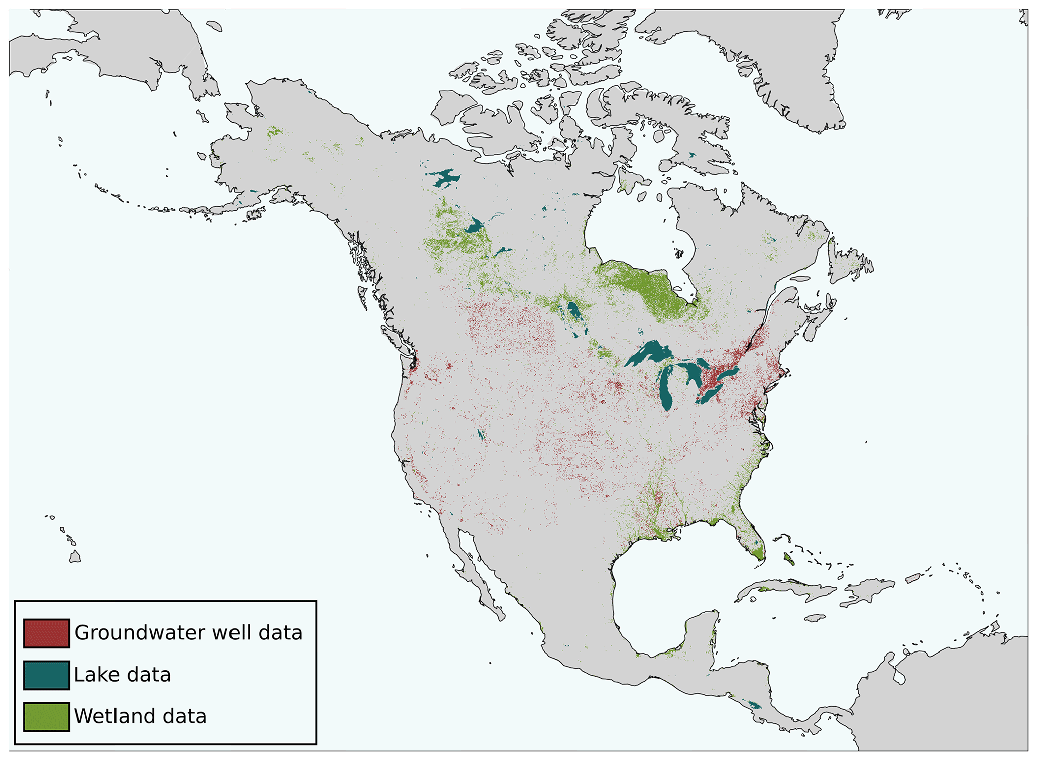
Figure F1 Location and spatial extent of each of the three data sources used to validate the depth to the water table.