Modelling rainfall with a Bartlett–Lewis process: pyBL (v1.0.0), a Python software package and an application with short records

The Bartlett–Lewis (BL) model is a stochastic framework for representing rainfall based upon Poisson cluster point process theory. This model has been used for over 30 years in the stochastic modelling of daily and hourly rainfall time series. Historically, the BL model was known to underestimate sub-daily rainfall extremes, but recent advancements have addressed this issue, making it a viable alternative to traditional rainfall frequency analysis methods, such as those based on annual maxima time series. Despite its potential, calibrating the BL model is a not a trivial task. The model's formulation is complex, and calibrating it involves a nonlinear optimisation process that can be numerically unstable, which has limited its broader application. To promote the use of the BL model and demonstrate its capabilities in modelling sub-hourly rainfall – both standard and extreme statistics – we have developed an open-source Python package called pyBL. This paper details the design of the BL model and summarises the key features of the pyBL package. It includes a brief explanation of how to use the package in selected user scenarios. In addition, we report on scientific experiments that resemble real-world situations to showcase pyBL's ability to model sub-hourly rainfall extremes with short records and its flexibility in utilising records of various timescales and lengths.

1 Introduction

Stochastic rainfall modelling is an increasingly popular technique used by the water and weather risk industries. It can be employed to synthesise sufficiently long rainfall time series to support hydrological applications, such as runoff and flood modelling (Koutsoyiannis et al., 2003; Gires et al., 2012; Kim et al., 2017a; Park et al., 2019), or weather-related risk analysis, such as the quantification of the impact of climate change (Onof and Arnbjerg-Nielsen, 2009; Cross et al., 2019; Kim and Onof, 2020; Papalexiou, 2022; Ebers et al., 2024).

The Bartlett–Lewis (BL) rectangular pulse model is a type of stochastic model that represents rainfall using a Poisson cluster point process to define the arrival of rectangular pulses representing short-duration constant intensity contributions to the cumulative rainfall. The model parameters are identified with standard statistical properties of rainfall data, such as mean, coefficient of variation, skewness, and autocovariance of the time series of rainfall depths at various important scales, as well the proportion of dry periods at those scales. Since the basic model type was published in 1987 (Rodriguez-Iturbe et al., 1987), several model variants have been developed (Rodriguez-Iturbe et al., 1988; Onof and Wheater, 1993; Onof et al., 2000; Kaczmarska et al., 2014; Onof and Wheater, 1994). In early versions, despite these models' ability to capture rainfall variability over a range of scales, two issues limiting their hydrological applicability have been commonly raised in the literature. First, BL models tend to underestimate hourly and sub-hourly extremes while overestimating daily extremes (Verhoest et al., 2010). Second, as identified by Marani (2003), BL models fail to reproduce rainfall variability for scales equal to or coarser than a few days. These limitations have been reported in many studies and pose significant challenges to the broader application of the BL model (see Verhoest et al., 2010, and references therein).

Recent advancements have addressed these issues, enhancing BL models' ability to preserve extreme statistics of rainfall at multiple timescales simultaneously (Cross et al., 2018; Onof and Wang, 2020; Kim and Onof, 2020). For example, Onof and Wang (2020) re-derived the analytical expressions for the rainfall depth moments in BL models and discovered that the parameter space is wider than was assumed in past studies. This relaxation of the parameter solution domain effectively improves BL models' capacity to preserve sub-hourly rainfall extremes. Furthermore, Kim and Onof (2020) extended Onof and Wang (2020)'s model by reorganising the temporal sequence of storms with a double shuffling algorithm. This enhances the model's ability to reproduce rainfall variability for scales ranging from a few days to a decade. In addition, preliminary studies suggest that the BL models are less sensitive to observational data length compared to existing rainfall frequency analysis methods that rely on, for example, annual maxima time series (Wang et al., 2020). Thus, it offers an alternative approach for modelling rainfall extremes when long datasets are not available.

In this work, we introduce an open-source Python package named pyBL. This package is implemented based on the state-of-the-art randomised BL model developed in Onof and Wang (2020) since this version of BL model is capable of not only reproducing standard statistical properties but also preserving extreme value statistics of rainfall across various timescales, from sub-hourly to daily. There are three main modules in the proposed pyBL package. These are the statistical property calculation module, the model fitting (i.e. calibration) module, and the sampling (i.e. simulation) module. The statistical property calculation module processes the input rainfall data and calculates its standard statistical properties at chosen timescales. The model fitting module calibrates the model parameters based upon the re-derived BL equations given in Onof and Wang (2020). To ensure efficient calibration and prevent the optimisation process from being trapped in local optima, a numerical solver employing the basin-hopping algorithm is implemented. Finally, the sampling module generates stochastic rainfall time series at a specified timescale and for any required data length based upon the fitted BL model.

The design of the BL is highly modularised, and the standard comma-separated value (CSV) format is used for file exchange between modules. Users can easily incorporate specific modules into their existing applications. In addition, a team comprising researchers from National Taiwan University and Imperial College London will consistently implement new advancements in BL models in the package, ensuring that users have access to the latest developments.

This paper is organised as follows. In Sect. 2, we provide detailed explanations of the formulation of the Bartlett–Lewis (BL) model. This includes a presentation of the model structure as well as an overview of model calibration and sampling processes. In addition, inspired by the bootstrapping method, we propose a novel approach to the estimation of model parameter uncertainty. Section 3 focuses on introducing the pyBL package. Specifically, we explain the workflow for using the package and summarise the pre-requisite Python packages needed to install pyBL. In Sect. 4, we use a case study to demonstrate and evaluate the BL model's ability to generate realistic rainfall time series. Two scenarios resembling data settings commonly found in many countries are designed and tested, showcasing the BL model's ability to produce rainfall extremes with short records. Finally, Sect. 5 summarises the key findings from this work and discusses potential further developments and applications of the proposed package.

2 Formulation of Bartlett–Lewis rectangular model

This section first explains the general structure of the BL model and the key adjustment in the most recent version of the model. Then, the processes of model calibration and of rainfall time series sampling is detailed. Finally, a method, inspired by the well-known bootstrapping method, is proposed here to estimate the model uncertainty.

2.1 Model structure

The model is constructed by a point process to represent the arrival of rainfall cells. This process is a Poisson cluster process which allows for the model to represent the observed clustering of such cells within longer rainfall events that are usually referred to as “storms”. As seen in Fig. 1, the storms therefore arrive as a Poisson process at rate λ. The clustering mechanism is that of the Bartlett–Lewis process. It involves the generation of a second Poisson process of rate β starting at the storm inception and of random duration, which we choose to be exponentially distributed with parameter γ.

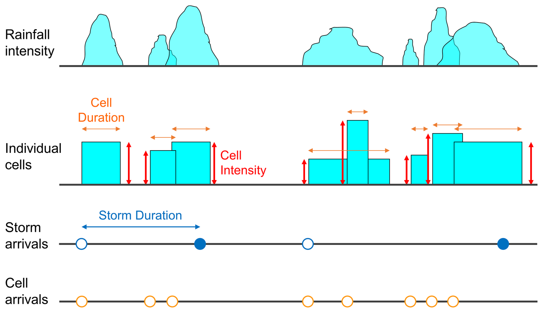
Figure 1 Conceptualisation of the Bartlett–Lewis rectangular pulse model (adapted from Fig. 1 in Onof and Wang, 2020).

The rainfall is then added to this point process: each cell is represented by a random rectangular pulse. This means that the rainfall intensity produced by each cell is random (with a distribution characterised by its first three non-centred moments μ_x,μ_x2, and μ_x3) but constant over the random duration of the cell. The latter is chosen as exponentially distributed with parameter η. Various cells will overlap, thereby producing a hyetograph that has a noisiness comparable to that of observed rainfall.

This describes the basic structure of a Bartlett–Lewis rectangular pulse model, which in its original version (Rodriguez-Iturbe et al., 1987) had all these distribution parameters define constant model parameters. It was, however, noted by Rodriguez-Iturbe et al. (1988), Onof and Wheater (1993), and others that a model in which the distribution parameters characterising the temporal structure of storms were allowed to vary from storm to storm would be preferable. This was achieved by randomising distribution parameter η: this becomes a random variable that is fixed for each storm but varies between storms and is Gamma distributed with shape parameter α and rate parameter ν, i.e. scale parameter $\mathrm{1}/\mathit{\nu }$. To ensure that all the temporal statistical features of storms scale in the same way, the cell arrival rate and the storm duration parameter are chosen as β=κη and γ=ϕη. This defines a randomised Bartlett–Lewis model which has been widely applied (e.g. Khaliq and Cunnane, 1996; Verhoest et al., 1997; Kim et al., 2017a, b; Kossieris et al., 2018).

A more recent version of the randomised Bartlett–Lewis model extends the randomisation to all the properties characterising the structure of the storm, i.e. also to the cell intensity parameters (Kaczmarska et al., 2014). So μ_x (and also μ_x2 and μ_x3 if a distribution other than the exponential is chosen for the cell intensity) is now a random variable that takes on a fixed value throughout a storm but which varies between storms proportionally to η. This defines a new model parameter ι such that μ_x=ιη. It is this randomised Bartlett–Lewis model (hereafter BL), as further developed by Onof and Wang (2020), that is coded up in pyBL.

2.2 Model calibration

The BL model is a continuous-time model, i.e. it defines a continuous-time stochastic process {Y(t)}_t∈ℝ, where Y(t) is the rainfall intensity at time t resulting from the superposition of the contributions of all the cells that are active at time t. Since rainfall data are generally available in discrete time, i.e. as a time series, the BL model can only be calibrated using the model's properties for rainfall aggregated to discrete timescales (e.g. h hours). These are properties of the discrete random variable defined at time step i by

$$\begin{array}{}\text{(1)}& Y_i^{\left(h\right)}=\underset{(i-\mathrm{1})h}{\overset{ih}{\int }}Y\left(t\right)\mathrm{d}t.\end{array}$$

It is not possible to obtain an analytical expression for the probability density function of $Y_i^{\left(h\right)}$ so that maximum likelihood estimation is not an option. What can be obtained are analytical expressions of the moments of the rainfall depth distribution (they are tractable up to the third order) of this variable (Onof and Wang, 2020) in terms of the model parameters and the timescale. Further, the probability of a dry interval at any timescale h, i.e. $P\left(Y_i^{\left(h\right)}\right)=\mathrm{0}$ can also be estimated (Onof and Wang, 2020). With these expressions, a generalised method of moments (Onof et al., 2000) is used to obtain parameters that produce values of these various properties that are as close as possible to their estimates from observed time series of rainfall depths. This defines an optimisation problem, which is the minimisation of the sum of the squares of the differences between analytical expressions of statistical model properties (the moments of the rainfall depth distribution or the proportion of dry periods at various timescales) as a function of model parameters and estimates of these properties from an observed time series:

$$\begin{array}{}\text{(2)}& \sum _{\mathcal{M}\in \mathrm{\Omega }}\mathit{\omega }\left(\mathcal{M}\right)\mathit{\{}\mathcal{M}-\widehat{\mathcal{M}}{\mathit{\}}}^{\mathrm{2}}.\end{array}$$

This minimisation is subject to certain feasibility constraints on the model parameters (Onof and Wang, 2020). In this expression, Ω is a set of statistical model properties, ω(ℳ) is a weight assigned to property ℳ (whose analytical expression is a function of the model parameters and the timescale) in the objective function, and $\widehat{\mathcal{M}}$ is the estimate of that same property from the observed time series. As discussed in Kaczmarska et al. (2014) and earlier works, the weight ω(ℳ) for a particular property is usually determined via the inverse variance weighting method. In other words, the inverse of the variance of the estimator for a given property is taken as the corresponding weight to reflect the estimator's reliability. If an estimator has a larger variance, indicating it is a less reliable representation of the true population statistic, then reproducing that property is assigned a lower priority.

Ultimately, the choice of which statistics to include in Ω will depend on which properties are deemed most important to reproduce, given the application for which the rainfall model is used. If the application does not obviously guide this choice, then Kaczmarska et al. (2014) recommend using the mean 1 h rainfall depth, and the coefficient of variation as well as the autocorrelation lag-1 and coefficient of skewness of rainfall depths at timescales of 1, 6, and 24 h (and also at sub-hourly scales if the data are available at such scales). These formulae for the BL model properties are provided in Appendix A.

Given the complexity of the BL model, determining optimal parameters is numerically challenging. Following the approach of Efstratiadis et al. (2002), calibration is treated as an optimisation problem that minimises the objective function in Eq. (2). While various strategies exist, such as the two-stage solver in Onof and Wang (2020) combining simulated annealing and the Nelder–Mead algorithm, in this implementation, a basin-hopping algorithm is utilised to reduce the likelihood of being trapped in local optima and help identify optimal parameters. As noted by Baioletti et al. (2024), basin hopping outperforms algorithms like differential evolution and particle swarm optimisation in terms of computational efficiency and solution accuracy. Our numerical solver runs basin hopping iteratively 20 times for each model calibration. The first iteration starts with a randomly assigned initial guess, while subsequent iterations use the solution from the previous basin-hopping iteration to refine the optimal solution.

Apart from the quality of the numerical solvers, the model's parameters are sensitive to factors such as data sample size and the estimation uncertainties of statistical properties. These influence the model's ability to reproduce observed statistics. Section S1 in the Supplement provides an in-depth sensitivity analysis, discussing the potential sources of uncertainty throughout the calibration process and offering readers an insight into challenges affecting the accuracy of the BL model.

2.3 Sampling

The sampling process of the BL model is fairly straightforward. It follows the concept of the BL model explained in Sect. 2.1. It involves two Poisson processes – one embedded in the other one – to model storm and rain cells, respectively. For each parameter set (usually corresponding to parameters for a given calendar month), the model first samples the number of storms based upon the specified sampling period (e.g. 10 years). For each storm event, the model then samples its arrival time and duration of activity (i.e. the time during which rain cells cam arrive) as well as the parameters associated with the distributions used to sample the properties of the embedded rain cells. Based upon the storm duration, the number of embedded rain cells is determined, and the arrival rates, durations, and intensities of these rain cells are sampled. It is worth mentioning that, to ensure the consistency of the starting time between a given storm and the corresponding cells, the starting time of the first cell has to align with that of the storm.

2.4 Modelling uncertainty

The uncertainty ranges from the above sampling process represent the sampling uncertainty, i.e. that arising from the variability between various samples of given size (i.e. length of the simulated time series). This is different from model parameter uncertainty, which is the uncertainty in the estimation of optimal model parameters. The sampling uncertainty can be decreased by extending the length of the simulation: it converges asymptotically to 0 as this length goes to infinity. The model parameter uncertainty, on the other hand, is a feature of the calibration process.

To model the parameter uncertainty of a BL model is no trivial task due to the complexity of its model structure. Here, a method, inspired by the bootstrap method (or bootstrapping), is proposed. Assuming the full record length is N years, one can randomly sample N years of data with replacement (that means data from any given year may be picked more than once) N_b times. Each N-year data sample is then used for BL model calibration, such that a total of N_b sets of BL parameters are obtained and used for sampling the corresponding time series with specified lengths. Based upon this bootstrapping process, the distribution of model parameters can be obtained, and thus model parameter uncertainty can be quantified.

The proposed method can be further extended if one wants to model the uncertainty resulting from the available data length. Instead of sampling N-year data, one can randomly sample N_s years of data with replacement (where N_s≤N) and proceed with the same process to model the corresponding uncertainty.

3 The pyBL package

As suggested by its name, the pyBL package is developed using the Python language. Python was chosen due to its open-source environment, extensive support libraries, and low learning curve, which facilitate the expansion of the pyBL user community. Here, we outline the complete workflow of running pyBL, starting from computing statistical properties from input rainfall records and fitting model parameters to sampling rainfall time series at a given timescale and length. In addition, we provide instructions for the usage of the package. The source code, example scripts, and test data for pyBL v1.1 can be downloaded from https://doi.org/10.5281/zenodo.12605935 (Wei et al., 2024), and please stay tuned with the further development at pyBL's GitHub repository: https://github.com/NTU-CompHydroMet-Lab/pyBL (last access: 30 May 2024).

3.1 Workflow

The workflow for using pyBL to build a BL model, sample rainfall time series, and calculate the associated statistics is illustrated in Fig. 2. As shown, it comprises five main steps. These are as follows:

1. User input. Users must provide two input files. The first file includes rainfall time series records as either a 1D array of rainfall intensity data or a 2D array including rainfall intensity data and associated timestamps. The second file is the model configuration file (Config), which allows users to control the entire modelling process.

2. Pre-processing. This step calculates the required statistical properties from the input rainfall records and estimates the associated “weights” for each property needed for BL model fitting (as mentioned in Sect. 2.2). Users can choose to export the calculation results to a CSV (comma-separated value) file for future use.

3. Model fitting. This step derives the BL model parameters based on the statistical properties and weights. As suggested by Onof and Wang (2020), a two-stage numerical minimisation strategy is used as the default solver. This strategy reduces the chance of the solution being trapped in a local optimum. The combination of dual-annealing and basin-hopping methods is implemented in this version of the package. The fitting process terminates when it reaches the error threshold or exceeds the iteration limit. Users can choose to export the fitted parameters to a CSV file for future use.

4. Sampling. This step uses the fitted BL model to sample rainfall time series, which preserves the statistical properties observed in the input records. The sampling process terminates when the required number of valid storms and cells are obtained. Users can choose to export the sampled storm and cell data to a JSON file for reference.

5. Post-processing. This step calculates standard and extreme statistics from the sampled time series to support model evaluation. Users can choose to export these statistical results to CSV files. In addition, users can choose to convert the raw storm and cell data into rainfall time series at a specified temporal resolution (e.g. 5 min or 1 h) and export it to a CSV file for subsequent hydrological applications.

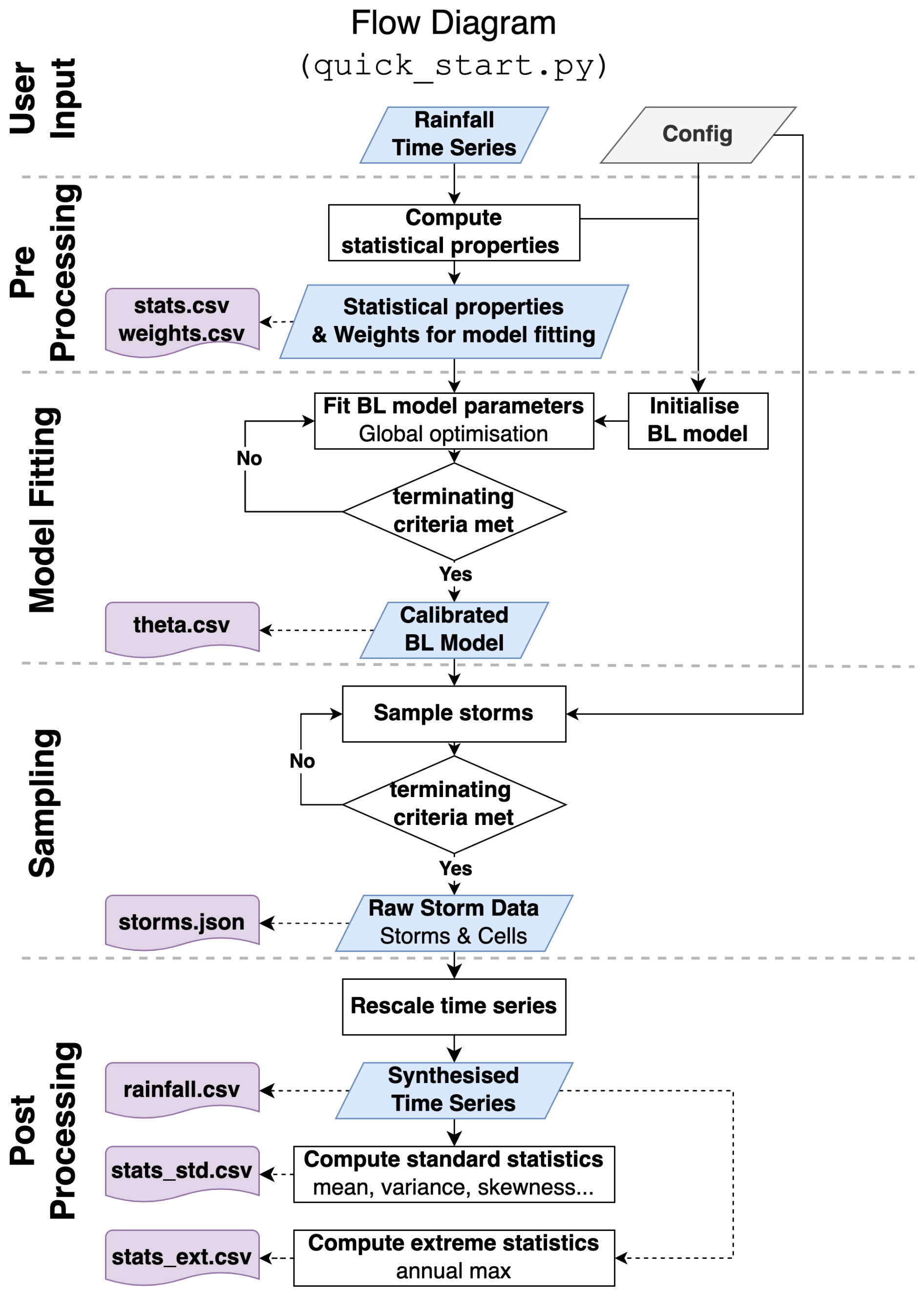
Figure 2 Workflow for generating synthetic rainfall time series using historical records with the pyBL package.

A Python notebook script, named quick_start.ipynb, is provided, accompanied by the package download (https://doi.org/10.5281/zenodo.12605935, Wei et al., 2024). This script enables users to run the entire workflow detailed above to stochastically generate rainfall time series with the test data. Notably, the package is designed to be highly modular, meaning that each of the above steps can be executed independently if the corresponding input is provided. For more examples, please refer to pyBL's GitHub repository (https://github.com/NTU-CompHydroMet-Lab, last access: 30 May 2024).

3.2 External libraries and package installation

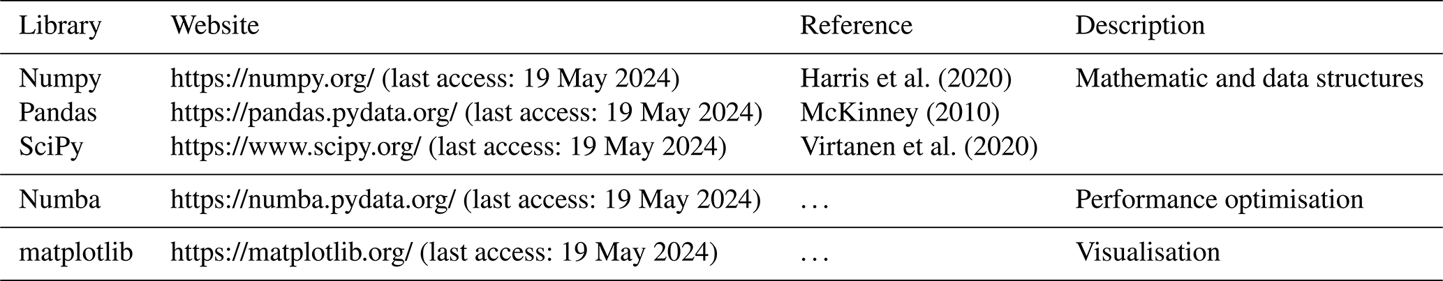
The implementation of pyBL depends on a number of external libraries. A list of these dependencies is summarised in Table 1. Amongst these libraries, Numpy and Pandas are used mainly for computing statistical properties from the input rainfall records. SciPy is used for BL model fitting. A robust numerical solver built on SciPy optimisers is used to obtain parameters for the pyBL model. Numba accelerates calculations using compiled C/C$++$ code, parallelisation, and CUDA kernels. Finally, matplotlib is an optional library for visualisation.

Harris et al. (2020)McKinney (2010)Virtanen et al. (2020)

Table 1 Summary of external libraries used by the pyBL package.

To install the pyBL package, it is recommended to use pip, which automatically resolves all dependencies and installs the pyBL package, simplifying the installation process for users.

4 Case study

In this section, we conduct experiments based on two scenarios that resemble real-world settings in many countries. In both scenarios, the extreme value performance of the BL model is compared with that of a conventional rainfall frequency analysis approach based on the annual maxima series and the generalised extreme value distribution (hereafter AM analysis). These two scenarios demonstrate that the BL model can not only serve as an alternative to conventional frequency analysis methods but also provide the flexibility to combine rainfall records at different temporal resolutions and recording periods.

4.1 Experimental design

4.1.1 Datasets

Rain gauge data at a 5 min timescale from a rain gauge in Bochum, Germany, are used to demonstrate the application of the pyBL package in this paper. The Bochum rainfall records used here span 69 years, from January 1931 to December 1999.

4.1.2 Scenarios

Two scenarios are designed here to resemble two real-world settings that can be found in many countries or regions in the world. These two scenarios are compared with a baseline, which represents a near-ideal setting where long sub-hourly rainfall data (over 30 years) are available.

These scenarios are

• Baseline (BS), which resembles a near-ideal setting where long (over 30 years) sub-hourly rainfall data are available. We use 5 min records over full recording periods from a gauge. This baseline scenario is to demonstrate that the BL model can be used as an alternative to the conventional AM analysis in modelling rainfall extremes.

• Scenario 1 (SC1), which resembles a widely seen setting in many regions where long-term rainfall records (for over 30 years) are not available. In this scenario, short records with different lengths (5, 10, 15, and 20 years) are used. The uncertainty ranges resulting from the BL model at various data lengths are compared with those from the traditional AM analysis. This scenario enables us to showcase the greater ability of the BL model to preserve extreme statistics with short records when compared with the traditional AM analysis.

• Scenario 2 (SC2), which resembles another relatively realistic setting seen in some countries. That is, sub-hourly rainfall records are available only in a shorter period (e.g. for 5–10 years), whilst hourly or coarser rainfall records are available for a longer period (i.e. for over 20 years). In this scenario, we would like to demonstrate that the BL model provides a flexible framework enabling the combination of rainfall records at different timescales with different data lengths.

4.1.3 Evaluation methods and metrics

The focus of the evaluation lies in the impact of modelling sub-hourly extreme statistics with short records. In Baseline, rainfall records at all timescales under consideration (i.e. 5 min and 1, 6, and 24 h) are randomly sampled with replacement for 69 years using the bootstrapping-inspired method described in Sect. 2.4 (where 100 bootstrapping iterations are conducted, i.e. N_b=100). In scenario 1 (SC1), instead of using full 69-year records, rainfall records at all timescales under consideration (i.e. 5 min and 1, 6, and 24 h) are randomly sampled with replacement for N years (with N=5, 10, 15, and 20) using the same bootstrapping method (where 100 bootstrapping iterations are conducted). In scenario 2 (SC2), we assume that full records are available for hourly or coarser timescales (i.e. 1, 6, and 24 h), and the statistical properties obtained from these records are combined with those derived from the N-year short records at the 5 min timescale for the simulation. Here, the last and the earliest N-year 5 min records from the original dataset are used (with N=5 and 20, respectively). The setup allows us to demonstrate how variations and uncertainties in short sub-hourly rainfall records affect the modelling process and impact the resulting extreme statistics.

In both SC1 and SC2 scenarios, we compare the return levels at T_r return periods (with $T_{\mathrm{r}}=\mathrm{20},\mathrm{50}$, and 100) with those derived from the base scenario (BS). In addition, for SC1, two widely used, non-dimensional, normalised evaluation metrics are utilised to quantify the estimation error of quantiles at T_r return periods. The first metric is to quantify the multiplicative bias between the estimated quantile resulting from the ith bootstrapping iteration $x_{\text{est}}^{i,T_{\mathrm{r}}}$ and the corresponding reference $x_{\text{ref}}^{T_{\mathrm{r}}}$, which is termed

$$\begin{array}{}\text{(3)}& {\mathrm{B}}^{i,T_{\mathrm{r}}}={\displaystyle \frac{x_{\text{est}}^{i,T_{\mathrm{r}}}}{x_{\text{ref}}^{T_{\mathrm{r}}}}},\end{array}$$

where bias (${\mathrm{B}}^{i,T_{\mathrm{r}}}$) ranges from 0 to +∞, with 1 indicating the perfect match. The second metric assesses the (relative) error between the estimated quantile and the corresponding reference at given return periods. This is done using the fractional standard error (FSE), which is termed

$$\begin{array}{}\text{(4)}& {\text{FSE}}^{T_{\mathrm{r}}}={\displaystyle \frac{\sqrt{\frac{\mathrm{1}}{N_{\mathrm{b}}}{\sum }_{i=\mathrm{1}}^{N_{\mathrm{b}}}{\left(x_{\text{est}}^{i,T_{\mathrm{r}}}-x_{\text{ref}}^{T_{\mathrm{r}}}\right)}^{\mathrm{2}}}}{x_{\text{ref}}^{T_{\mathrm{r}}}}},\end{array}$$

where FSE ranges from 0 to +∞, with 0 representing no error.

4.2 Results and discussion

4.2.1 Modelling rainfall with full records (Baseline)

Before discussing the “short-record” scenarios, we first present the results of the Baseline model. Full 69-year records from Bochum were used for calibration, and the fitted parameters for each calendar month are summarised in Table 2. These parameters align closely with previous studies using the same dataset (see Table 4 in Onof and Wang, 2020). In addition, using these parameters and the bootstrapping method from Sect. 2.4, we derived statistical properties of rainfall at various timescales, which closely match the observed. As shown in Figs. 3–6, the Baseline model (green boxplots, denoted RBL) well preserves key properties such as mean rainfall depth; coefficient of variation; autocorrelation lag-1; and skewness at 5 min and 1, 6, and 24 h (1 d) timescales.

Table 2 Parameters for the BL model using Bochum gauge data with full records.

Figure 3 Mean by month at Bochum. Comparison between RBL (boxes) and observations (crosses).

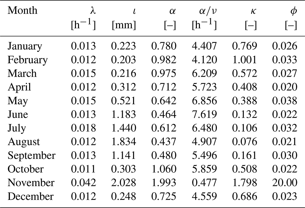
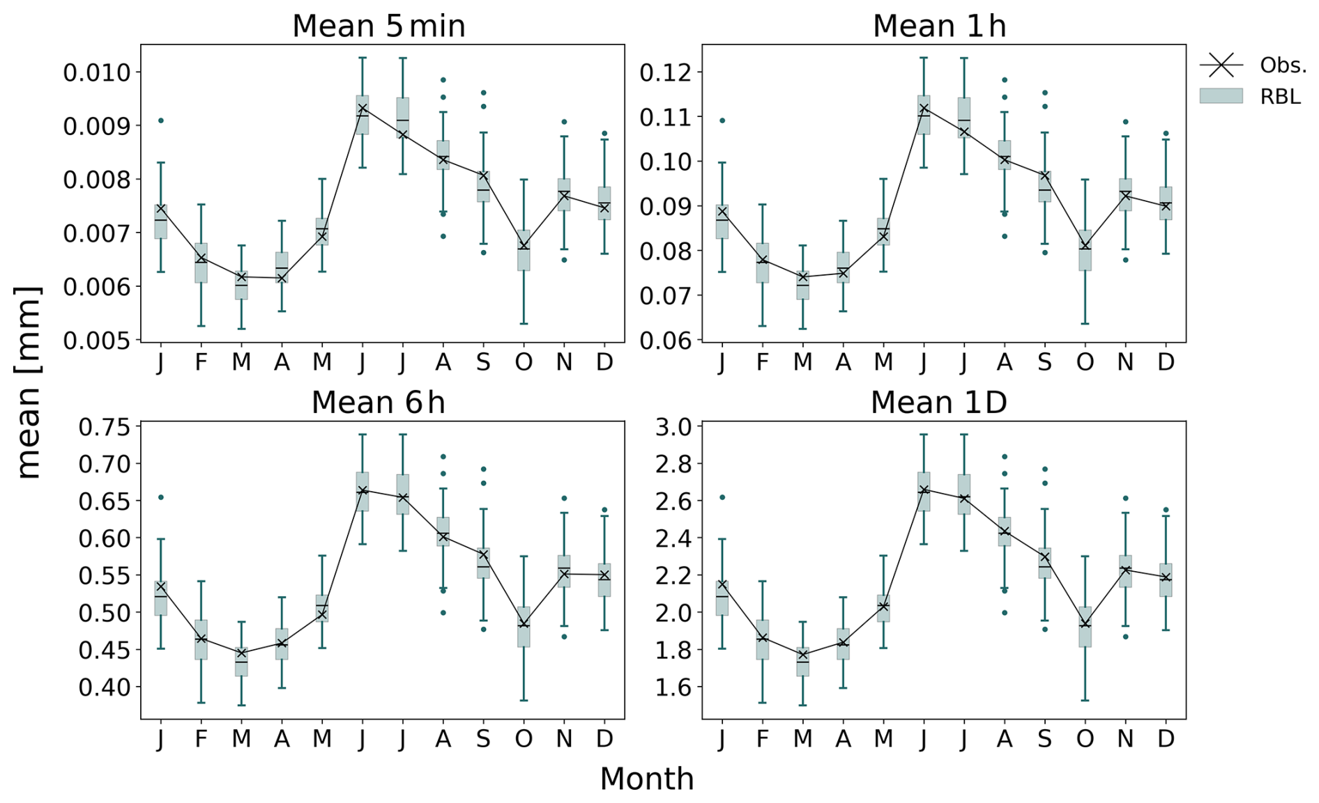
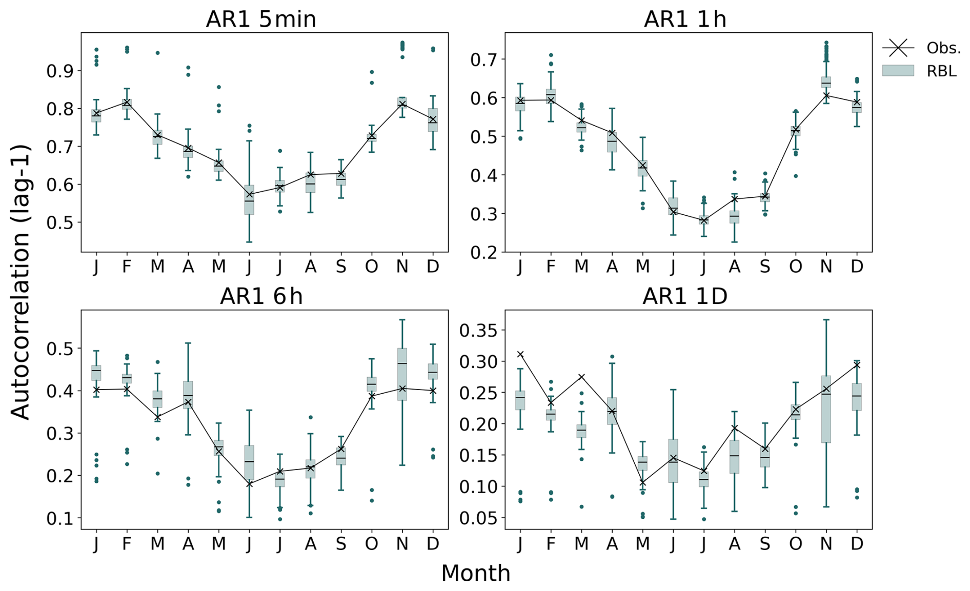
Figure 4 Autocorrelation lag-1 (AR1) by month at Bochum. Comparison between RBL (boxes) and observations (crosses).

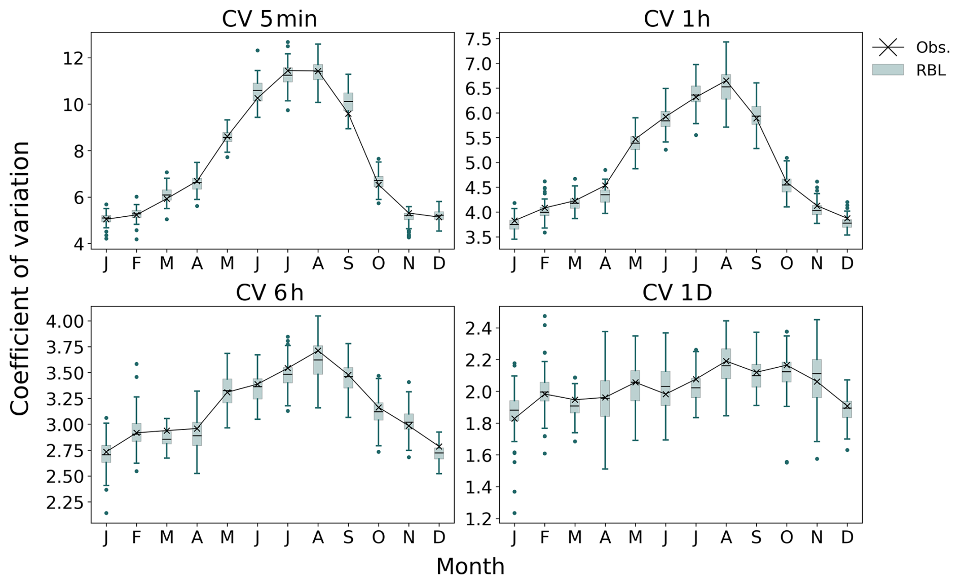
Figure 5 Coefficient of variation (CV) by month at Bochum. Comparison between RBL (boxes) and observations (crosses).

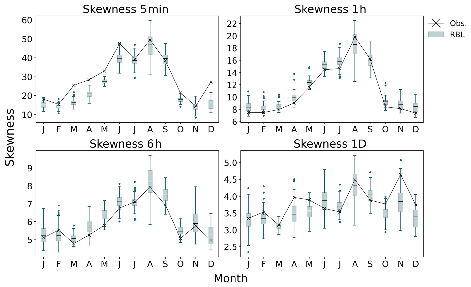
Figure 6 Skewness by month at Bochum. Comparison between RBL (boxes) and observations (crosses).

However, when investigating properties at the 1-month (labelled 1 M) timescale (see Fig. 7), we find that the current Baseline model, implemented in pyBL, can only reproduce monthly rainfall means but fails to preserve inter-monthly variability. This limitation arises because these monthly properties are not considered during model calibration. Addressing this issue is critical for certain applications, such as drought studies, and a future version of the BL model could integrate methods, such as the shuffling components proposed by Kim and Onof (2020), to better account for monthly rainfall variability.

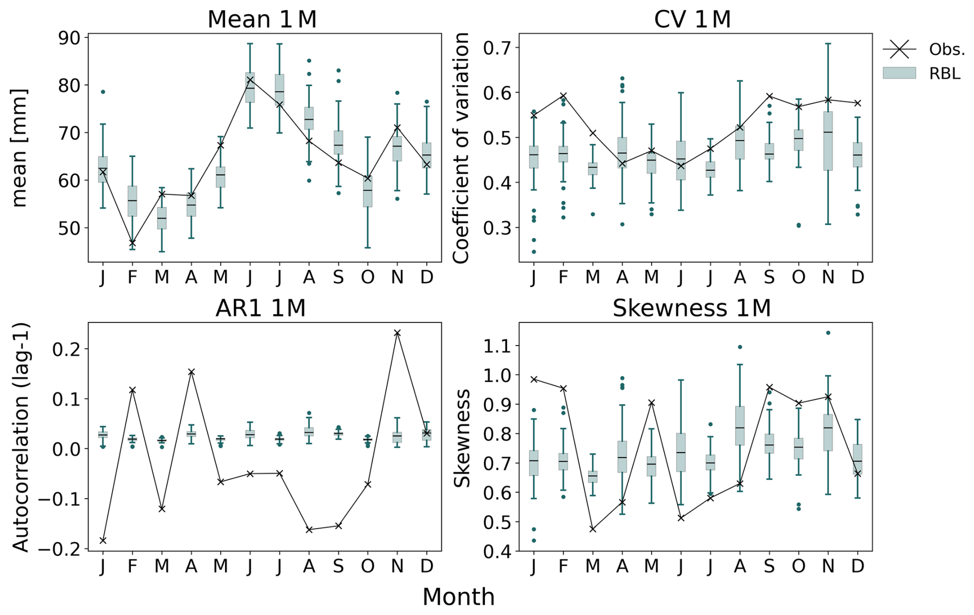
Figure 7 Selected statistical properties in 1 M timescale by month at Bochum. Comparison between RBL (boxes) and observations (crosses).

4.2.2 Modelling rainfall with short records (SC1)

Here, we focus on assessing the hourly and sub-hourly rainfall extremes with various data lengths. In Fig. 8, return levels at 5 min (left column of plots) and 1 h (right column of plots) timescales obtained from the BL model (green boxplots, denoted RBL) and the AM analysis (yellow boxplots, denoted AM (GEV)) are given, respectively. From top to bottom rows, the return level estimates for 20-, 50-, and 100-year return periods are given. Each plot presents the estimates resulting from rainfall records with 5-, 10-, 15-, and 20-year data lengths and full records (FR, i.e. 69 years).

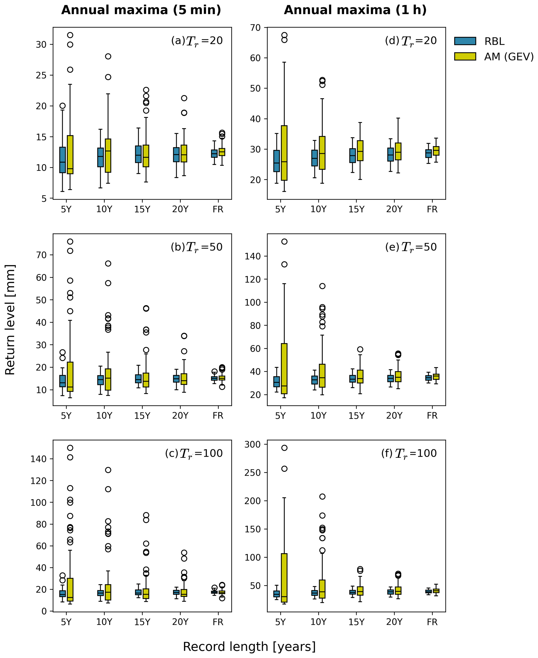
Figure 8 Boxplots of 5 min and 1 h return levels from RBL (blue boxes) and AM analysis (yellow boxes) for different record lengths (5, 10, 15, and 20 years and full records) at 20-, 50-, and 100-year return periods (top to bottom).

As seen in the plots, the median estimates of the return levels from the BL model generally align with those from the AM analysis. Nonetheless, the uncertainty ranges are significantly different, with those from the BL model being much smaller than those from the AM analysis. The difference is particularly evident as the records are short, and the targeted return periods are high. Moreover, the BL model results in far fewer outliers compared to the AM analysis. Notably, for the 100-year 5 min return levels, the uncertainty range from the BL model fitted with 20-year records is similar to that from the AM analysis fitted with full records (69 years). Similar observations can be made for the 100-year 1 h return levels (see Fig. 8f).

The quality of the return level estimation and the corresponding uncertainty can be further quantified using the bias (B) and the FSE measures. Figure 9a and c compare the (multiplicative) biases of the 5 min and 1 h return levels, resulting from the BL model and the AM analysis against the reference return levels (i.e. those estimated from the full records). The full quantile intervals are used to represent uncertainty ranges.

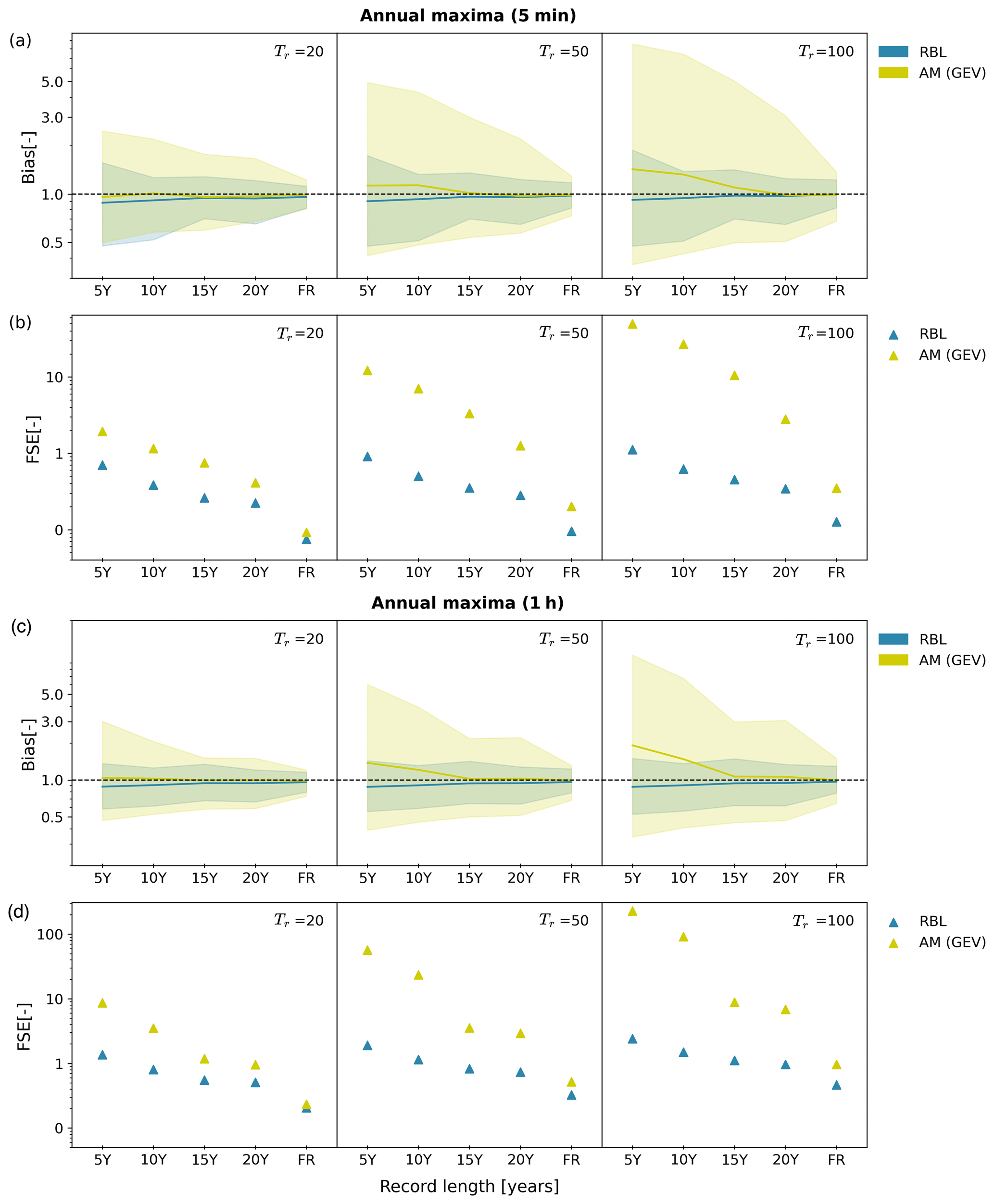
Figure 9 Comparisons of 20-, 50-, and 100-year return levels at 5 min (a, b) and 1 h (c, d) timescales derived from the BL model (denoted RBL) and AM analysis (denoted AM (GEV)) using 5-, 10-, 15-, and 20-year short records, as well as full records (69 years). Multiplicative biases and fractional standard errors (FSEs) of each member of 100 bootstrapping iterations are calculated against the reference values, and the full quantile intervals are presented.

From the median estimates (solid blue lines), it is evident that the BL model tends to slightly underestimate the return levels, particularly when the rainfall records are shorter than 15–20 years. This underestimation is consistent across both 5 min and 1 h timescales and for all return periods examined. However, the uncertainty ranges are adequate to cover the unbiased line (B=1.0, dashed dark lines). The median estimates from the AM analysis (solid yellow lines) exhibit a different behaviour. While the AM analysis appears to provide more unbiased estimates at relatively low return periods (T_r=20) compared to the BL model, a significant overestimation is observed at higher return periods, especially with records shorter than 15 years. In addition, the AM analysis results in much larger uncertainty ranges than the BL model when records are shorter than 20 years, with the size of these ranges increasing drastically as return periods become higher. Unlike the AM analysis, the uncertainty ranges resulting from the BL model remain relatively stable across all return periods examined.

This difference in uncertainty ranges is further highlighted in the FSE estimates (see Fig. 9b and d). The FSE estimates from the BL model remain consistently similar as return periods increase, whereas those from the AM analysis increase significantly, particularly when records are shorter than 15–20 years.

To summarise results of the SC1 experiment, the BL model shows itself able to preserve extreme rainfall statistics at 5 min and 1 h timescales even though extreme rainfall records are not used for model calibration. Moreover, its estimation uncertainty of the extreme statistics is significantly less sensitive to record lengths as compared to the traditional AM analysis. This robustness can be attributed to the fact that the BL model works with standard statistics calculated from the entire rainfall records rather than just the annual maximum data, which represents a small subset of the records. Consequently, the BL model proves to be a robust alternative to the AM analysis, particularly when only short records are available.

4.2.3 Modelling rainfall with short sub-hourly records

Following the SC1 with short-record analysis, we now shift our focus to a SC2 setting where hourly (or coarser-resolution) rainfall data are available for 69 years, whilst sub-hourly rainfall data are available for only 5 years (the most recent 5-year period being 1995–1999). Here, we compare the 5 min rainfall extremes derived from the traditional AM analysis and the BL model. The associated uncertainty is calculated using the bootstrapping method detailed in Sect. 2.4, with the full quantile intervals representing the estimation uncertainty ranges.

As illustrated in Fig. 10, we first observe that the dashed dark line, representing median estimates of 5 min extremes from the AM analysis (denoted AM (GEV)-5y, 5min), is nearly horizontal (with negligible increase) after the 10-year return period. In addition, the associated uncertainty range grows exponentially after the same return period. This is likely caused by fitting the GEV distribution with a very small dataset, which is numerically challenging. The BL model effectively addresses this issue and results in more reasonable estimates of 5 min extremes (see yellow line, denoted RBL-5y, 5min). Moreover, the uncertainly interval is significantly reduced compared to that from the AM analysis. This result is consistent with that in SC1.

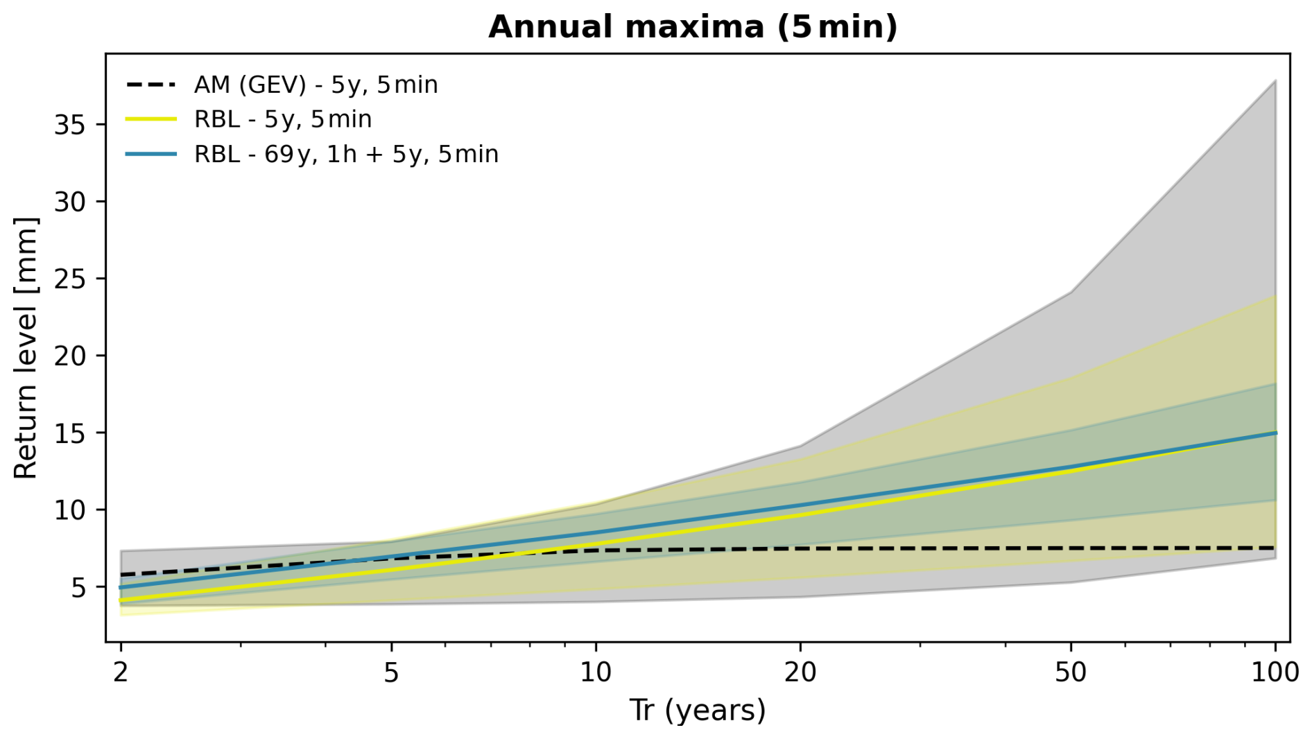
Figure 10 Comparison of 5 min return levels for 2- to 100-year return periods, with estimation uncertainty. Traditional AM analysis (dashed dark line, grey shading), BL model using 5 years of 5 min data (solid yellow line and shading), and BL model calibrated with 5 years of 5 min data and 69 years of 1 h records (solid blue line and shading).

We then further calibrate the BL model using the aforementioned SC2 setting, i.e. using 5-year 5 min data and the 69-year 1 h data (see blue line, denoted RBL-69y, 1h + 5y, 5min). This combination results in similar median estimates to those from the RBL model with 5 years of 5 min data only but leads to a further reduction in the uncertainty range. This highlights the capacity of the BL model to integrate data at different timescales and lengths, adding value to short sub-hourly rainfall records.

The benefit of integrating data at different timescales and lengths can be further explored from another perspective. It has been observed in the literature that the impact of climate change on rainfall patterns varies across different timescales. Specifically, many studies have noted that increases in temperature lead to more pronounced variations in rainfall extremes at finer timescales (e.g. sub-hourly or hourly) compared to coarser timescales (e.g. multiple-hourly or daily) (Chan et al., 2016; Fowler et al., 2021; Huang et al., 2022; Cannon et al., 2024). In other words, the level of statistical non-stationarity is different for rainfall at different timescales – that is, generally higher for sub-hourly rainfall and lower for hourly or coarser-scale rainfall. Given that the data used to construct a BL model are assumed to be statistically stationary, it makes sense to calibrate BL models using data at different timescales and lengths to better comply with the stationary assumption and to more accurately represent underlying rainfall features.

To further explore this multi-timescale perspective, we continue with the SC2 setting but introduce some minor changes. Specifically, we combine 1 h full records with 5 min data from different periods – the earliest or the most recent 5/20 years – to reflect the impact on fine-scale rainfall extremes, caused by the non-stationarity in the sub-hourly rainfall time series. The reason for choosing these two periods lies in the variations in 5 min rainfall extremes observed between them. As illustrated in Fig. 11, the 69-year 5 min annual maxima from 1931 to 1999 are presented. As highlighted in the plot, there is a notable difference in annual maxima between the earliest (1931–1935, blue shading) and the most recent (1995–1999, yellow shading) 5 years, where the average difference is over 2 mm. This difference is, however, largely reduced if we extend the average from 5 to 20 years.

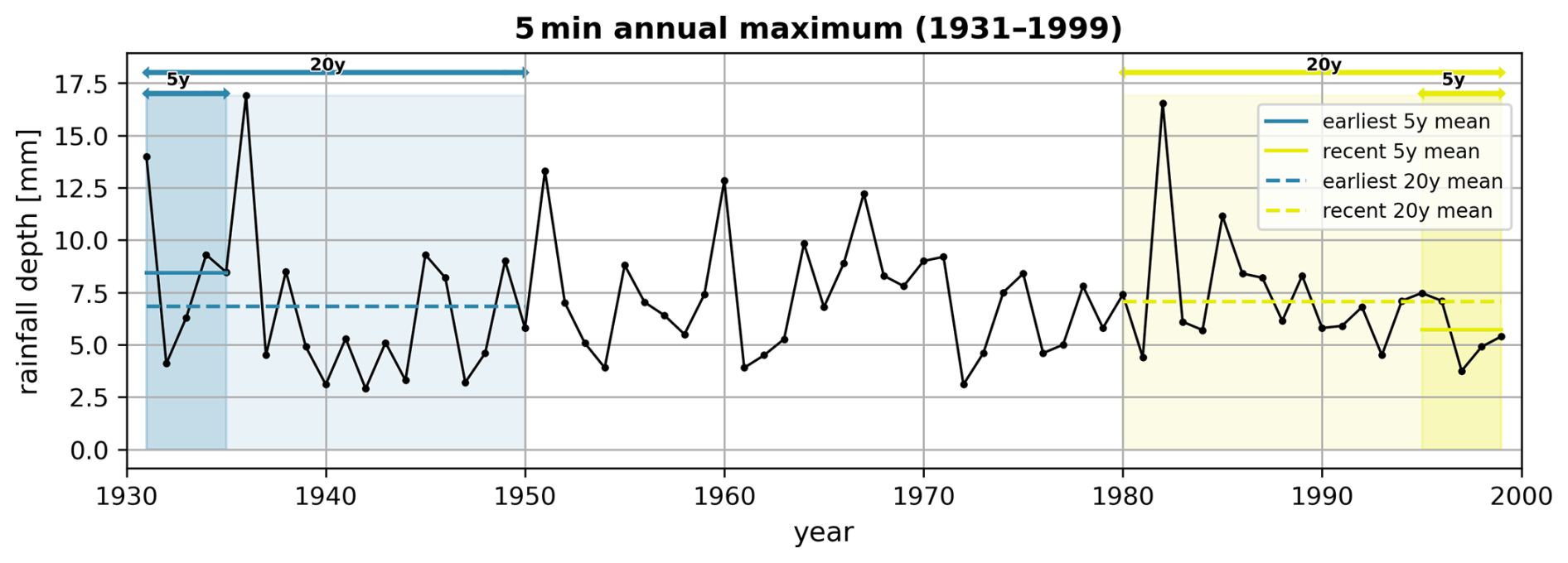
Figure 11 Data for 5 min annual maximum rainfall records at Bochum (1931–1999) are shown (solid dark line). Average values for the earliest 5 and 20 years (blue lines and shading) and most recent 5 and 20 years (yellow lines and shading) highlight significant differences in extreme statistics over these periods.

We find that this “dynamics” observed for the 5 min rainfall extremes effectively propagate through the BL modelling. As shown in Fig. 12 (upper left), the BL model calibrated with 69-year 1 h data and the earliest 5-year 5 min data (see light blue boxes) results in much higher 5 min extremes compared to those calibrated with 69-year 1 h data and the most recent 5-year 5 min data (see blue boxes). This relative difference observed in the sampled 5 min return levels aligns with that presented in Fig. 11, where the average of the 5 min annual maxima over the earliest 5 years is much higher than that over the most recent 5 years. Please note that, in this experiment, all results presented come from the BL modelling, so the variations in uncertainty ranges caused by different models is not our main evaluation focus. Thus, the bootstrapping method is not conducted here for model uncertainty estimation. The uncertainty ranges presented here come from the sampling process.

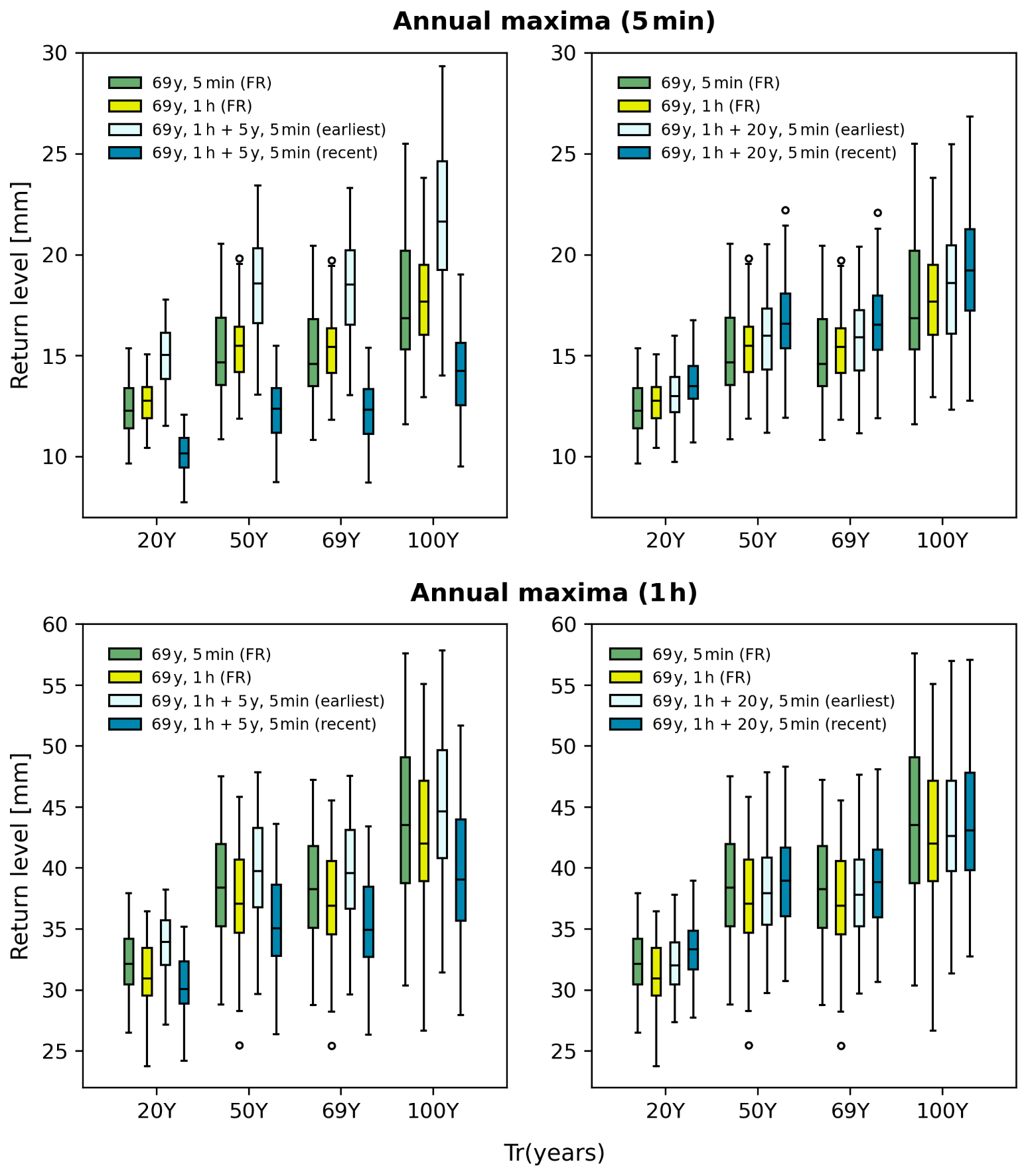
Figure 12 Boxplots of 5 min and 1 h return levels from the BL model calibrated with various data settings, including 69-year 5 min data (full records, green boxes: 69y, 5-min (FR)), 69-year 1 h data without 5 min data (yellow boxes: 69y, 1 h (FR)), 69-year 1 h data with the earliest 5/20 years of 5 min data (light-blue boxes: 69y, 1 h + 5/20y, 5 min (earliest)), and 69-year 1 h data with the most recent 5/20 years of 5 min data (blue boxes: 69y, 1 h + 5/20y, 5 min (recent)). Return levels for 20-, 50-, 69- (full records), and 100-year periods are shown.

We also observe that the difference in annual maxima is largely reduced at the 1 h timescale (see Fig. 12, lower left), as well as when the available 5 min records increase from 5 to 20 years (see Fig. 12, upper right). The former, together with the result presented in Fig. 12 (upper left), demonstrates that the BL model not only reflects the variations in sub-hourly rainfall extremes but also effectively maintains the stationarity in hourly rainfall extremes. The latter, however, showcases that the variations in sub-hourly rainfall extremes may be smoothed out when a longer time period of data is used.

To summarise the results of the SC2 experiment, we demonstrate the flexibility of the BL model in working with rainfall data at different timescales and lengths, highlighting the corresponding benefits. Specifically, the BL model can effectively reduce the estimation uncertainty in sub-hourly rainfall extreme calculations by integrating long hourly data with short sub-hourly records. In addition, it offers a straightforward approach to account for the varying impacts of climate dynamics on rainfall properties across different timescales.

5 Conclusions

This work introduces an open-source Python package named pyBL for generating rainfall time series using randomised Bartlett–Lewis rectangular pulse models (BL models). Historically, BL models have been effective in producing rainfall time series with realistic statistical properties across various timescales. However, they have also been known to underestimate rainfall extremes at sub-daily timescales. Recent advancements have addressed this issue, enabling the BL model to preserve both standard and extreme statistics at sub-hourly and hourly timescales while maintaining its ability to generate realistic rainfall features (Kaczmarska et al., 2014; Onof and Wang, 2020).

Implementing the BL model is a challenging task due to its complex formulation and the nonlinear optimisation required to derive its parameters. To overcome these challenges and promote the widespread use of the BL model, we developed pyBL. This paper provides explanations of its structure and installation instructions. In addition, we explored a potential application of the BL model with two scenarios that mimic real-world situations where only short sub-hourly records are available.

In the first scenario (SC1), we demonstrate that the BL model can produce robust sub-hourly and hourly rainfall extremes with short records. Compared to conventional annual maximum analysis, the BL model achieves similar consistency in estimating sub-hourly rainfall extremes with only half the record length (or even shorter).

In the second scenario (SC2), we showcase the BL model's flexibility in integrating rainfall records at different timescales and lengths. We demonstrated that the estimation uncertainty in sub-hourly rainfall extremes, when using only short sub-hourly records, can be significantly reduced by incorporating long hourly records. In addition, the BL model provides a straightforward method to account for the varying impacts of climate dynamics on rainfall properties across different timescales.

These findings suggest that the BL model is a viable alternative to traditional annual maximum analysis, especially for short records. Its ability to work with short records and integrate data of varying lengths is advantageous for regions with limited high-resolution rainfall records, maximising the utility of their data. In addition, it opens the door to other applications. For example, recent developments by Islam et al. (2022) and Islam et al. (2023) highlight the potential of applying the BL model to satellite-derived IMERG (Integrated Multi-satellite Retrievals for Global Precipitation Measurement mission) rainfall products.

However, the current implementation does have limitations. Notably, it struggles to reproduce properties other than the mean at the monthly timescale, which restricts its use for applications requiring that large-scale variability be reproduced. Future improvements could include methods akin to the shuffling components proposed by Kim and Onof (2020) in which an additional parameter was introduced to better handle storm dependence at monthly scales. In addition, for model calibration, the ability to employ various weighting schemes might be incorporated into future versions of the pyBL package. This enhancement would provide greater flexibility for specific hydrological applications, which require putting more weight on some rather than other statistics.

The pyBL package developed in this work will not only help countries overcome the barrier of short records but also accelerate the exploration of various applications. By providing a robust and flexible tool for rainfall time series generation, pyBL can facilitate a more accurate and comprehensive analysis of rainfall extremes, which is crucial for water resource management, urban planning, and climate impact studies. The package's ability to integrate different timescales and lengths of data will particularly benefit regions with limited historical rainfall data, enabling them to make informed decisions based on more reliable rainfall statistics.

Appendix A: Formulae for fitting properties

The complete formulae are given here for the selected statistical moments based upon different parameter ranges. These include mean, variance, lag-k autocovariance, and the third central moment of the discrete time-aggregated process of the version of the Bartlett–Lewis model implemented in pyBL (v1.0.0).

The definitions of the model parameters used are given below:

• h is the timescale,

• λ is the storm arrival rate,

• α is the shape parameter for the Gamma distribution of the cell termination rate (η),

• ν is the scale parameter for the Gamma distribution of η,

• κ is the ratio of the cell arrival rate to η (i.e. $\mathit{\beta }/\mathit{\eta }$),

• ϕ is the ratio of the storm termination rate to η (i.e. $\mathit{\gamma }/\mathit{\eta }$),

• ι is the ratio of mean cell intensity to η (i.e. ${\mathit{\mu }}_X/\mathit{\eta }$),

• $f_{\mathrm{1}}={\mathit{\mu }}_{X^{\mathrm{2}}}/{\mathit{\mu }}_X^{\mathrm{2}}$,

• $f_{\mathrm{2}}={\mathit{\mu }}_{X^{\mathrm{3}}}/{\mathit{\mu }}_X^{\mathrm{3}}$,

• ${\mathit{\mu }}_C=\mathrm{1}+\mathit{\kappa }/\mathit{\varphi }$ is the mean number of cells per storm.

Mean

$$\begin{array}{}\text{(A1)}& M\left(h\right)=\mathit{\lambda }h\mathit{\iota }{\mathit{\mu }}_c\end{array}$$

Variance

$$\begin{array}{}\text{(A2)}& \begin{array}{rl}V\left(h\right)=& \mathrm{2}\mathit{\lambda }{\mathit{\mu }}_c{\mathit{\iota }}^{\mathrm{2}}\left[\right(f_{\mathrm{1}}+{\displaystyle \frac{\mathit{\kappa }}{\mathit{\varphi }}})h\\ & +({\displaystyle \frac{\mathit{\kappa }(\mathrm{1}-{\mathit{\varphi }}^{\mathrm{3}})}{{\mathit{\varphi }}^{\mathrm{2}}({\mathit{\varphi }}^{\mathrm{2}}-\mathrm{1})}}-f_{\mathrm{1}})T(\mathrm{1},\mathrm{0},\mathrm{0})\\ & -\left({\displaystyle \frac{\mathit{\kappa }}{{\mathit{\varphi }}^{\mathrm{2}}({\mathit{\varphi }}^{\mathrm{2}}-\mathrm{1})}}\right)T(\mathrm{1},\mathit{\varphi }h,\mathrm{0})\\ & +(f_{\mathrm{1}}+{\displaystyle \frac{\mathit{\kappa }\mathit{\varphi }}{{\mathit{\varphi }}^{\mathrm{2}}-\mathrm{1}}})T(\mathrm{1},h,\mathrm{0})]\\ & \text{ for }\mathit{\alpha }>\mathrm{1},\\ V\left(h\right)\approx & \mathrm{2}\mathit{\lambda }{\mathit{\mu }}_c{\mathit{\iota }}^{\mathrm{2}}\left[{\displaystyle \frac{{\mathit{\eta }}_{\mathrm{0}}^{\mathit{\alpha }+\mathrm{1}}{h}^{\mathrm{2}}{\mathit{\nu }}^{\mathit{\alpha }}}{\mathrm{2}(\mathit{\alpha }+\mathrm{1})\mathrm{\Gamma }\left(\mathit{\alpha }\right)}}\right({\displaystyle \frac{\mathit{\kappa }}{\mathit{\varphi }+\mathrm{1}}}+f_{\mathrm{1}})\\ & +(f_{\mathrm{1}}+{\displaystyle \frac{\mathit{\kappa }}{\mathit{\varphi }}})hT(\mathrm{0},\mathrm{0},{\mathit{\eta }}_{\mathrm{0}})\\ & +({\displaystyle \frac{\mathit{\kappa }(\mathrm{1}-{\mathit{\varphi }}^{\mathrm{3}})}{{\mathit{\varphi }}^{\mathrm{2}}({\mathit{\varphi }}^{\mathrm{2}}-\mathrm{1})}}-f_{\mathrm{1}})T(\mathrm{1},\mathrm{0},{\mathit{\eta }}_{\mathrm{0}})\\ & -\left({\displaystyle \frac{\mathit{\kappa }}{{\mathit{\varphi }}^{\mathrm{2}}({\mathit{\varphi }}^{\mathrm{2}}-\mathrm{1})}}\right)T(\mathrm{1},\mathit{\varphi }h,{\mathit{\eta }}_{\mathrm{0}})\\ & +(f_{\mathrm{1}}+{\displaystyle \frac{\mathit{\kappa }\mathit{\varphi }}{{\mathit{\varphi }}^{\mathrm{2}}-\mathrm{1}}})T(\mathrm{1},h,{\mathit{\eta }}_{\mathrm{0}})]\\ & \text{ for }-\mathrm{1}<\mathit{\alpha }\le \mathrm{1}.\end{array}\end{array}$$

Covariance at lag k≥1

$$\begin{array}{}\text{(A3)}& \begin{array}{rl}C(k,h)=& \mathit{\lambda }{\mathit{\mu }}_c{\mathit{\iota }}^{\mathrm{2}}\mathit{\left\{}\right(f_{\mathrm{1}}+{\displaystyle \frac{\mathit{\kappa }\mathit{\varphi }}{{\mathit{\varphi }}^{\mathrm{2}}-\mathrm{1}}}\left)\right[T(\mathrm{1},(k-\mathrm{1})h,\mathrm{0})\\ & -\mathrm{2}T(\mathrm{1},kh,\mathrm{0})+T(\mathrm{1},(k+\mathrm{1})h,\mathrm{0})]\\ & -\left({\displaystyle \frac{\mathit{\kappa }}{{\mathit{\varphi }}^{\mathrm{2}}({\mathit{\varphi }}^{\mathrm{2}}-\mathrm{1})}}\right)\left[T\right(\mathrm{1},\mathit{\varphi }(k-\mathrm{1})h,\mathrm{0})\\ & -\mathrm{2}T(\mathrm{1},\mathit{\varphi }kh,\mathrm{0})+T(\mathrm{1},\mathit{\varphi }(k+\mathrm{1})h,\mathrm{0})\left]\mathit{\right\}}\\ & \text{ for }\mathit{\alpha }>\mathrm{1},\\ C(k,h)\approx & \mathit{\lambda }{\mathit{\mu }}_c{\mathit{\iota }}^{\mathrm{2}}\mathit{\left\{}{\displaystyle \frac{{\mathit{\eta }}_{\mathrm{0}}^{\mathit{\alpha }+\mathrm{1}}{h}^{\mathrm{2}}{\mathit{\nu }}^{\mathit{\alpha }}}{\mathrm{\Gamma }\left(\mathit{\alpha }\right)(\mathit{\alpha }+\mathrm{1})}}\right(f_{\mathrm{1}}+{\displaystyle \frac{\mathit{\kappa }}{\mathit{\varphi }+\mathrm{1}}})\\ & +(f_{\mathrm{1}}+{\displaystyle \frac{\mathit{\kappa }\mathit{\varphi }}{{\mathit{\varphi }}^{\mathrm{2}}-\mathrm{1}}})\left[T\right(\mathrm{1},(k-\mathrm{1})h,{\mathit{\eta }}_{\mathrm{0}})\\ & -\mathrm{2}T(\mathrm{1},kh,{\mathit{\eta }}_{\mathrm{0}})+T(\mathrm{1},(k+\mathrm{1})h,{\mathit{\eta }}_{\mathrm{0}})]\\ & -\left({\displaystyle \frac{\mathit{\kappa }}{{\mathit{\varphi }}^{\mathrm{2}}({\mathit{\varphi }}^{\mathrm{2}}-\mathrm{1})}}\right)\left[T\right(\mathrm{1},\mathit{\varphi }(k-\mathrm{1})h,{\mathit{\eta }}_{\mathrm{0}})\\ & -\mathrm{2}T(\mathrm{1},\mathit{\varphi }kh,{\mathit{\eta }}_{\mathrm{0}})+T(\mathrm{1},\mathit{\varphi }(k+\mathrm{1})h,{\mathit{\eta }}_{\mathrm{0}})\left]\mathit{\right\}}\\ & \text{ for }-\mathrm{1}<\mathit{\alpha }\le \mathrm{1}.\end{array}\end{array}$$

Third central moment

$$\begin{array}{}\text{(A4)}& \begin{array}{rl}S\left(h\right)=& {\displaystyle \frac{\mathit{\lambda }{\mathit{\mu }}_c{\mathit{\iota }}^{\mathrm{3}}{\sum }_{k=\mathrm{1}}^{k=\mathrm{8}}{P}_k(\mathit{\varphi },\mathit{\kappa },f_{\mathrm{1}},f_{\mathrm{2}},\mathrm{0})}{(\mathrm{1}+\mathrm{2}\mathit{\varphi }+{\mathit{\varphi }}^{\mathrm{2}})({\mathit{\varphi }}^{\mathrm{4}}-\mathrm{2}{\mathit{\varphi }}^{\mathrm{3}}-\mathrm{3}{\mathit{\varphi }}^{\mathrm{2}}+\mathrm{8}\mathit{\varphi }-\mathrm{4}){\mathit{\varphi }}^{\mathrm{3}}}}\\ & \text{ for }\mathit{\alpha }>\mathrm{1},\\ S\left(h\right)\approx & {\displaystyle \frac{\mathit{\lambda }{\mathit{\mu }}_c{\mathit{\iota }}^{\mathrm{3}}}{(\mathrm{1}+\mathrm{2}\mathit{\varphi }+{\mathit{\varphi }}^{\mathrm{2}})({\mathit{\varphi }}^{\mathrm{4}}-\mathrm{2}{\mathit{\varphi }}^{\mathrm{3}}-\mathrm{3}{\mathit{\varphi }}^{\mathrm{2}}+\mathrm{8}\mathit{\varphi }-\mathrm{4}){\mathit{\varphi }}^{\mathrm{3}}}}\\ & \left[{\displaystyle \frac{{\mathit{\nu }}^{\mathit{\alpha }}{\mathit{\eta }}_{\mathrm{0}}^{\mathit{\alpha }+\mathrm{2}}{h}^{\mathrm{3}}}{\mathrm{\Gamma }\left(\mathit{\alpha }\right)(\mathit{\alpha }+\mathrm{2})}}\right(\mathrm{2}{\mathit{\kappa }}^{\mathrm{2}}({\mathit{\varphi }}^{\mathrm{7}}-\mathrm{3}{\mathit{\varphi }}^{\mathrm{6}}+{\mathit{\varphi }}^{\mathrm{5}}+\mathrm{3}{\mathit{\varphi }}^{\mathrm{4}}-\mathrm{2}{\mathit{\varphi }}^{\mathrm{3}})\\ & +f_{\mathrm{2}}({\mathit{\varphi }}^{\mathrm{9}}-\mathrm{6}{\mathit{\varphi }}^{\mathrm{7}}+\mathrm{9}{\mathit{\varphi }}^{\mathrm{5}}-\mathrm{4}{\mathit{\varphi }}^{\mathrm{3}})\\ & +\mathrm{3}\mathit{\kappa }{f}_{\mathrm{1}}({\mathit{\varphi }}^{\mathrm{8}}-{\mathit{\varphi }}^{\mathrm{7}}-\mathrm{5}{\mathit{\varphi }}^{\mathrm{6}}+\mathrm{5}{\mathit{\varphi }}^{\mathrm{5}}+\mathrm{4}{\mathit{\varphi }}^{\mathrm{4}}-\mathrm{4}{\mathit{\varphi }}^{\mathrm{3}}))\\ & +\sum _{k=\mathrm{1}}^{k=\mathrm{8}}{P}_k(\mathit{\varphi },\mathit{\kappa },f_{\mathrm{1}},f_{\mathrm{2}},{\mathit{\eta }}_{\mathrm{0}})]\\ & \text{ for }-\mathrm{2}<\mathit{\alpha }\le \mathrm{1},\end{array}\end{array}$$

with

$$\begin{array}{c}{\displaystyle }\begin{array}{rl}{P}_{\mathrm{1}}& (\mathit{\varphi },\mathit{\kappa },f_{\mathrm{1}},f_{\mathrm{2}},l)=\mathrm{6}T(\mathrm{1},h,l){\mathit{\varphi }}^{\mathrm{2}}\\ & \times \left[\mathit{\varphi }{\mathit{\kappa }}^{\mathrm{2}}\right(\mathrm{2}{\mathit{\varphi }}^{\mathrm{4}}-\mathrm{7}{\mathit{\varphi }}^{\mathrm{2}}-\mathrm{3}\mathit{\varphi }+\mathrm{2})\\ & +\mathrm{2}\mathit{\varphi }{f}_{\mathrm{2}}({\mathit{\varphi }}^{\mathrm{6}}-\mathrm{6}{\mathit{\varphi }}^{\mathrm{4}}+\mathrm{9}{\mathit{\varphi }}^{\mathrm{2}}-\mathrm{4})\\ & +\mathit{\kappa }{f}_{\mathrm{1}}(\mathrm{4}{\mathit{\varphi }}^{\mathrm{6}}-\mathrm{22}{\mathit{\varphi }}^{\mathrm{4}}-{\mathit{\varphi }}^{\mathrm{3}}+\mathrm{25}{\mathit{\varphi }}^{\mathrm{2}}+\mathrm{4}\mathit{\varphi }-\mathrm{4})],\end{array}\\ {\displaystyle }\begin{array}{rl}{P}_{\mathrm{2}}& (\mathit{\varphi },\mathit{\kappa },f_{\mathrm{1}},f_{\mathrm{2}},l)=\mathrm{6}T(\mathrm{0},h,l){\mathit{\varphi }}^{\mathrm{3}}h\\ & \times \left[f_{\mathrm{2}}\right({\mathit{\varphi }}^{\mathrm{6}}-\mathrm{6}{\mathit{\varphi }}^{\mathrm{4}}+\mathrm{9}{\mathit{\varphi }}^{\mathrm{2}}-\mathrm{4})+\mathit{\varphi }\mathit{\kappa }{f}_{\mathrm{1}}({\mathit{\varphi }}^{\mathrm{2}}-\mathrm{1}\left)\right({\mathit{\varphi }}^{\mathrm{2}}-\mathrm{4}\left)\right],\end{array}\\ {\displaystyle }\begin{array}{rl}{P}_{\mathrm{3}}& (\mathit{\varphi },\mathit{\kappa },f_{\mathrm{1}},f_{\mathrm{2}},l)=\mathrm{6}T(\mathrm{1},\mathit{\varphi }h,l)\mathit{\kappa }\\ & \times \left[f_{\mathrm{1}}\right(-{\mathit{\varphi }}^{\mathrm{5}}+{\mathit{\varphi }}^{\mathrm{4}}+\mathrm{6}{\mathit{\varphi }}^{\mathrm{3}}-\mathrm{4}{\mathit{\varphi }}^{\mathrm{2}}-\mathrm{8}\mathit{\varphi })\\ & +\mathit{\kappa }({\mathit{\varphi }}^{\mathrm{5}}-\mathrm{3}{\mathit{\varphi }}^{\mathrm{4}}+\mathrm{2}{\mathit{\varphi }}^{\mathrm{3}}+\mathrm{14}{\mathit{\varphi }}^{\mathrm{2}}-\mathrm{8})],\end{array}\\ {\displaystyle }{P}_{\mathrm{4}}(\mathit{\varphi },\mathit{\kappa },f_{\mathrm{1}},f_{\mathrm{2}},l)=\mathrm{6}T(\mathrm{0},\mathit{\varphi }h,l)h{\mathit{\kappa }}^{\mathrm{2}}\left[{\mathit{\varphi }}^{\mathrm{3}}\right(\mathrm{5}-{\mathit{\varphi }}^{\mathrm{2}})-\mathrm{4}\mathit{\varphi }],\\ {\displaystyle }\begin{array}{rl}{P}_{\mathrm{5}}& (\mathit{\varphi },\mathit{\kappa },f_{\mathrm{1}},f_{\mathrm{2}},l)=T(\mathrm{1},\mathrm{0},l)\\ & \times [-\mathrm{12}{\mathit{\varphi }}^{\mathrm{3}}{f}_{\mathrm{2}}({\mathit{\varphi }}^{\mathrm{6}}-\mathrm{6}{\mathit{\varphi }}^{\mathrm{4}}+\mathrm{9}{\mathit{\varphi }}^{\mathrm{2}}-\mathrm{4})\\ & +{\mathit{\kappa }}^{\mathrm{2}}(-\mathrm{9}{\mathit{\varphi }}^{\mathrm{7}}+\mathrm{39}{\mathit{\varphi }}^{\mathrm{5}}+\mathrm{18}{\mathit{\varphi }}^{\mathrm{4}}-\mathrm{12}{\mathit{\varphi }}^{\mathrm{3}}-\mathrm{84}{\mathit{\varphi }}^{\mathrm{2}}+\mathrm{48})\\ & -\mathrm{3}\mathit{\varphi }\mathit{\kappa }{f}_{\mathrm{1}}(\mathrm{7}{\mathit{\varphi }}^{\mathrm{7}}-\mathrm{39}{\mathit{\varphi }}^{\mathrm{5}}-\mathrm{2}{\mathit{\varphi }}^{\mathrm{4}}+\mathrm{46}{\mathit{\varphi }}^{\mathrm{3}}+\mathrm{12}{\mathit{\varphi }}^{\mathrm{2}}-\mathrm{8}\mathit{\varphi }-\mathrm{16})],\end{array}\\ {\displaystyle }\begin{array}{rl}{P}_{\mathrm{6}}& (\mathit{\varphi },\mathit{\kappa },f_{\mathrm{1}},f_{\mathrm{2}},l)=T(\mathrm{0},\mathrm{0},l)\\ & \times \left[\right(\mathrm{6}h{\mathit{\varphi }}^{\mathrm{3}}{f}_{\mathrm{2}}+\mathrm{12}h{\mathit{\varphi }}^{\mathrm{2}}\mathit{\kappa }{f}_{\mathrm{1}}+\mathrm{6}h\mathit{\varphi }{\mathit{\kappa }}^{\mathrm{2}})\\ & \times ({\mathit{\varphi }}^{\mathrm{6}}-\mathrm{6}{\mathit{\varphi }}^{\mathrm{4}}+\mathrm{9}{\mathit{\varphi }}^{\mathrm{2}}-\mathrm{4})],\end{array}\\ {\displaystyle }\begin{array}{rl}{P}_{\mathrm{7}}& (\mathit{\varphi },\mathit{\kappa },f_{\mathrm{1}},f_{\mathrm{2}},l)=\mathrm{3}T(\mathrm{1},\mathrm{2}h,l){\mathit{\varphi }}^{\mathrm{4}}(\mathrm{1}-{\mathit{\varphi }}^{\mathrm{2}}){\mathit{\iota }}^{\mathrm{3}}\\ & \times [\mathit{\varphi }{\mathit{\kappa }}^{\mathrm{2}}+\mathit{\kappa }{f}_{\mathrm{1}}({\mathit{\varphi }}^{\mathrm{2}}-\mathrm{4}\left)\right],\end{array}\\ {\displaystyle }\begin{array}{rl}{P}_{\mathrm{8}}& (\mathit{\varphi },\mathit{\kappa },f_{\mathrm{1}},f_{\mathrm{2}},l)=\mathrm{6}T(\mathrm{1},(\mathrm{1}+\mathit{\varphi })h,l)\mathit{\kappa }{\mathit{\varphi }}^{\mathrm{2}}(\mathit{\varphi }-\mathrm{2})(\mathit{\varphi }-\mathrm{1}){\mathit{\iota }}^{\mathrm{3}}\\ & \times \left[f_{\mathrm{1}}\right(\mathit{\varphi }+\mathrm{2})-\mathit{\varphi }\mathit{\kappa }].\end{array}\end{array}$$