Explaining neural networks for detection of tropical cyclones and atmospheric rivers in gridded atmospheric simulation data

Detection of atmospheric features in gridded datasets from numerical simulation models is typically done by means of rule-based algorithms. Recently, the feasibility of learning feature detection tasks using supervised learning with convolutional neural networks (CNNs) has been demonstrated. This approach corresponds to semantic segmentation tasks widely investigated in computer vision. However, while in recent studies the performance of CNNs was shown to be comparable to human experts, CNNs are largely treated as a “black box”, and it remains unclear whether they learn the features for physically plausible reasons. Here we build on the recently published “ClimateNet” dataset that contains features of tropical cyclones (TCs) and atmospheric rivers (ARs) as detected by human experts. We adapt the explainable artificial intelligence technique “Layer-wise Relevance Propagation” (LRP) to the semantic segmentation task and investigate which input information CNNs with the Context-Guided Network (CGNet) and U-Net architectures use for feature detection. We find that both CNNs indeed consider plausible patterns in the input fields of atmospheric variables. For instance, relevant patterns include point-shaped extrema in vertically integrated precipitable water (TMQ) and circular wind motion for TCs. For ARs, relevant patterns include elongated bands of high TMQ and eastward winds. Such results help to build trust in the CNN approach. We also demonstrate application of the approach for finding the most relevant input variables (TMQ is found to be most relevant, while surface pressure is rather irrelevant) and evaluating detection robustness when changing the input domain (a CNN trained on global data can also be used for a regional domain, but only partially contained features will likely not be detected). However, LRP in its current form cannot explain shape information used by the CNNs, although our findings suggest that the CNNs make use of both input values and the shape of patterns in the input fields. Also, care needs to be taken regarding the normalization of input values, as LRP cannot explain the contribution of bias neurons, accounting for inputs close to zero. These shortcomings need to be addressed by future work to obtain a more complete explanation of CNNs for geoscientific feature detection.

1 Introduction

The automated detection and tracking of 2-D and 3-D atmospheric features including cyclones, fronts, jet streams, or atmospheric rivers (ARs) in simulation and observation data has multiple applications in meteorology. For example, automatically detected features are used for weather forecasting (e.g., Hewson and Titley, 2010; Mittermaier et al., 2016; Hengstebeck et al., 2018), statistical and climatological studies (e.g., Dawe and Austin, 2012; Pena-Ortiz et al., 2013; Schemm et al., 2015; Sprenger et al., 2017; Lawrence and Manney, 2018), and visual data analysis (e.g., Rautenhaus et al., 2018; Bösiger et al., 2022; Beckert et al., 2023). Features are typically detected based on a set of physical and mathematical rules. For example, cyclones can be identified by searching for minima or maxima in variables including mean sea level pressure and lower-tropospheric vorticity (Neu et al., 2013; Bourdin et al., 2022). Atmospheric fronts can be identified by means of derivatives of a thermal variable combined with threshold-based filters (Jenkner et al., 2010; Hewson and Titley, 2010; Beckert et al., 2023) and ARs based on thresholding and geometric requirements (Guan and Waliser, 2015; Shields et al., 2018).

Recent research has shown that, given a pre-defined labeled dataset, supervised learning with artificial neural networks (ANNs), in particular convolutional neural networks (CNNs), can learn a feature detection task. For example, Kapp-Schwoerer et al. (2020) and Prabhat et al. (2021) (abbreviated as KS20 and P21 hereafter) showed that CNNs can be trained to detect tropical cyclone (TC) and AR features. Lagerquist et al. (2019), Biard and Kunkel (2019), Niebler et al. (2022), and Justin et al. (2023) used CNNs to detect atmospheric fronts. In these works, CNNs are used to classify individual grid points of a gridded input dataset according to whether they belong to a feature. This corresponds to a “semantic segmentation task” widely investigated in the computer vision literature for segmentation and classification of regions in digital images, e.g., cars, trees, or road surface (Long et al., 2015; Liu et al., 2019; Xie et al., 2021; Manakitsa et al., 2024).

Using CNNs for feature detection via semantic segmentation can have several advantages. These include increased computational performance (Boukabara et al., 2021; Higgins et al., 2023) and the option to learn features that are difficult to formulate as a set of physical rules (P21; Niebler et al., 2022; Tian et al., 2023). A major limiting factor, however, is that they are “black box” algorithms that do not allow for an easy interpretation of the decision-making process inside CNNs. Hence, one does not know whether a CNN bases its decision on plausible patterns in the data. If not, a CNN may still perform well on the training data but fails to generalize to unseen data (Lapuschkin et al., 2019). To approach this issue, the artificial intelligence (AI) community has proposed methods for explainable artificial intelligence (xAI) in the past decade (Linardatos et al., 2021; Holzinger et al., 2022; Mersha et al., 2024). Examples include Layer-wise Relevance Propagation (LRP; Bach et al., 2015), Local Interpretable Model-Agnostic Explanations (LIME; Ribeiro et al., 2016), Gradient-weighted Class Activation Mapping (Grad-CAM; Selvaraju et al., 2017), and Shapley Additive Explanations (SHAP; Lundberg and Lee, 2017). In short, these methods provide information about what an ANN “looks at” when computing its output, hence allowing evaluation of the plausibility of the learned patterns.

The xAI methods vary with respect to several characteristics. For example, the relevance of the input data can be computed per input grid point¹ or for entire regions of the input data and per input variable² or jointly for all variables. Also, the complexity of implementation differs. For application in semantic segmentation, an open challenge is also that existing xAI methods have been mainly developed for classification tasks, i.e., for CNNs assigning input data to one of several classes (instead of identifying the spatial structure of a feature, this corresponds to the following question: “is a particular feature contained in the input data?”). While Grad-CAM is readily available for use with semantic segmentation (Captum, 2023; MathWorks, 2023), it has the drawback of not being able to differentiate between input variables (Selvaraju et al., 2017). SHAP can be implemented for semantic segmentation (e.g., Dardouillet et al., 2023); however, it computes relevance values for clusters of input grid points and not for individual input grid points. The same applies to LIME; moreover, to the best of our knowledge, we are not aware of implementations of LIME for semantic segmentation. The feasibility of using LRP for semantic segmentation has been demonstrated in the context of medical imaging (Tjoa et al., 2019; Ahmed and Ali, 2021), and it produces relevance information per grid point and input variable.

Our goal for the study at hand is to provide an xAI method that works with semantic segmentation CNNs trained to detect atmospheric features. We are interested in opening the “black box” to investigate whether a CNN uses physically plausible input patterns to make its decision. This requires analysis of the spatial distribution of input relevance (i.e., which regions and structures are relevant for a particular feature; hence relevance information per grid point is needed), as well as analysis of distributions of relevant input variables (i.e., which values of which input variables are of importance to detect a feature; hence relevance information per input variable are needed).

As an application example, we consider the work by KS20 and P21, who introduced an expert-labeled dataset of TCs and ARs in atmospheric simulation data (the “ClimateNet” dataset). KS20 and P21 trained two different CNN architectures, DeepLabv3+ (Chen et al., 2018) and Context-Guided Network (CGNet; Wu et al., 2021), to perform feature detection via semantic segmentation. The studies showed that for the given task, the CNNs learned to detect TCs and ARs and that the CGNet architecture outperformed the DeepLabv3+ architecture. However, in neither study was an xAI technique applied.

Mamalakis et al. (2022) (abbreviated as M22 hereafter) recently presented work in this direction by reformulating the P21 segmentation task into a classification task and evaluating several available xAI techniques for classification, including LRP and SHAP. They considered subregions of the global dataset used by P21 and differentiated whether zero, one, or more ARs exist in a subregion. TCs were not considered. M22 showed that for their classification setup, LRP yielded useful information to assess the plausibility of the decision-making inside the CNN. LRP has also been successfully applied in further geoscientific studies concerned with use of CNNs for classification tasks (Beobide-Arsuaga et al., 2023; Davenport and Diffenbaugh, 2021; Labe and Barnes, 2022; Toms et al., 2020). It also fulfills our requirement of computing relevance information per grid point and input variable (at least in some variants; cf. M22).

In this study, we build on the work by KS20, P21, and M22. We demonstrate and analyze the use of LRP for the KS20/P21 case of detecting TCs and ARs, using the CGNet architecture used by KS20 and the ClimateNet dataset provided by P21 (Sect. 2). We reproduce the KS20/P21 setup (Sect. 3) and address the following objectives:

1. Adapt LRP to the semantic segmentation task for geoscientific datasets and extend the method to be applicable to the CGNet CNN architecture (Sect. 4).

2. Examine the plausibility of spatial relevance patterns and distributions of relevant inputs for TC and AR detection as computed with LRP (Sects. 5 and 6).

3. Demonstrate further applications of LRP for semantic segmentation, including assessment of the most relevant input variables for a feature detection task and assessment of the robustness of feature detection when data of subregions instead of global data are used as input (Sect. 7).

For comparison and due to its widespread use for semantic segmentation in computer vision, we also consider the U-Net architecture (Ronneberger et al., 2015). To limit paper length, however, its results are mainly presented in the Supplement.

2 The ClimateNet dataset

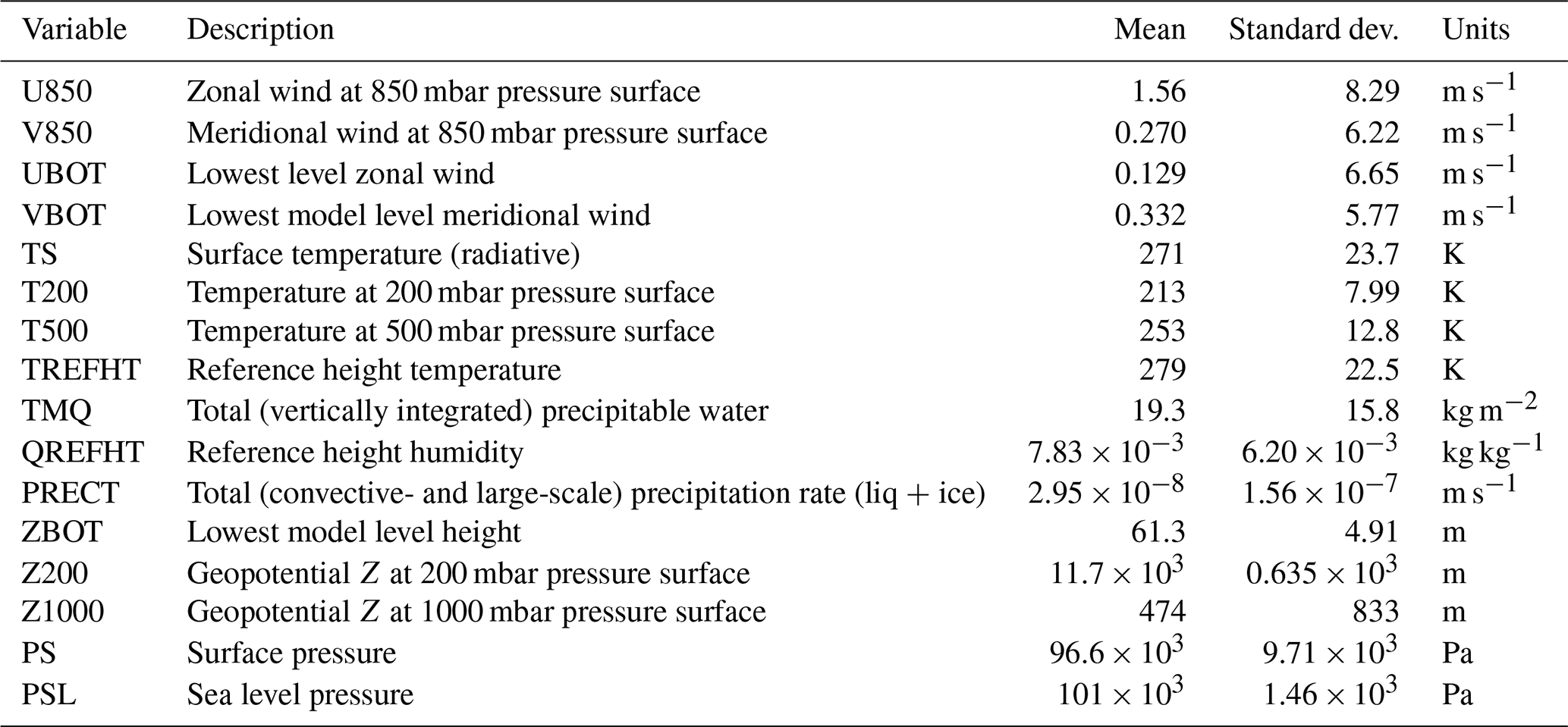
The ClimateNet dataset introduced by P21 contains global 2-D longitude–latitude grids of selected atmospheric variables at a collection of time steps from a simulation conducted with the Community Atmospheric Model (CAM5.1; Wehner et al., 2014), spanning a time interval from 1996 to 2013 (note that these are not reanalysis data). Each grid has a size of 768×1152 grid points and contains 16 variables, listed in Table 1. Experts labeled 219 time steps, assigning each grid point to one of three classes: background (BG), TC, and AR. An individual feature is represented by connected grid points of the same class. As most time steps were labeled by multiple experts, the dataset contains 459 input–output mappings, with sometimes very different labels for the same input data. As P21 argued, these disagreements in classifications reflect the diversity in views and assumptions by different experts. P21 split the labeled data into a training (398 mappings) and test dataset (61 mappings) by taking all time steps prior to 2011 as training data and all other as test data.

Following KS20, we apply z-score normalization on each variable to set the mean values to 0 and the standard deviations to 1, hence achieving equally distributed inputs. As discussed by LeCun et al. (2012), this normalization reduces the convergence time of CNNs during training. Also, z-score normalization helps to treat all input variables as equally important by a CNN (e.g., Chase et al., 2022). An issue when using LRP (and other xAI methods; cf. M22) with z-score-normalized data, however, is the “ignorant-to-zero-input issue” discussed by M22: zero input values are assigned zero relevance. We will discuss the impact of this issue on the usefulness of the LRP results. For comparison, we also discuss results obtained by training the CNNs using a min–max normalization (which rescales the variable values to the range [0, 1]; e.g., García et al., 2014) and a modified z-score normalization shifted by a value of +10 in the normalized data domain (the mean value becomes +10; the standard deviation remains 1).

Table 1 Atmospheric 2-D fields (variables) contained in the P21 ClimateNet dataset. Variable short names are used throughout the text.

3 Reproduction of the KS20/P21 task with CGNet and U-Net

Following KS20/P21, we formulate the detection of TCs and ARs as a semantic segmentation task, with the goal of assigning one of the classes TC, AR, or BG to every grid point. We evaluate the CGNet (Wu et al., 2021; shown by KS20 to outperform the DeepLabv3+ architecture used by P21) and U-Net (Ronneberger et al., 2015) CNN architectures. Figure 1 illustrates both architectures. CNNs are a class of ANNs that capture spatial patterns by successively convolving the data with spatially local kernels (e.g., Russell and Norvig, 2021). For semantic segmentation tasks, CNNs compute a probability value for each grid point and class as output. U-Net features an encoder–decoder architecture that first successively decreases the grid size to detect high-level patterns at different scales using convolutional layers, followed by upsampling and a combination of the extracted patterns leading to segmentation as output. To improve the quality of the segmentation, skip connections between the respective levels of the encoder and decoder are introduced. In contrast, CGNet uses a typical classification-style CNN architecture (Simonyan and Zisserman, 2015) without a dedicated decoder. It uses context guided blocks that combine spatially local patterns with larger-scale patterns to produce a final segmentation.

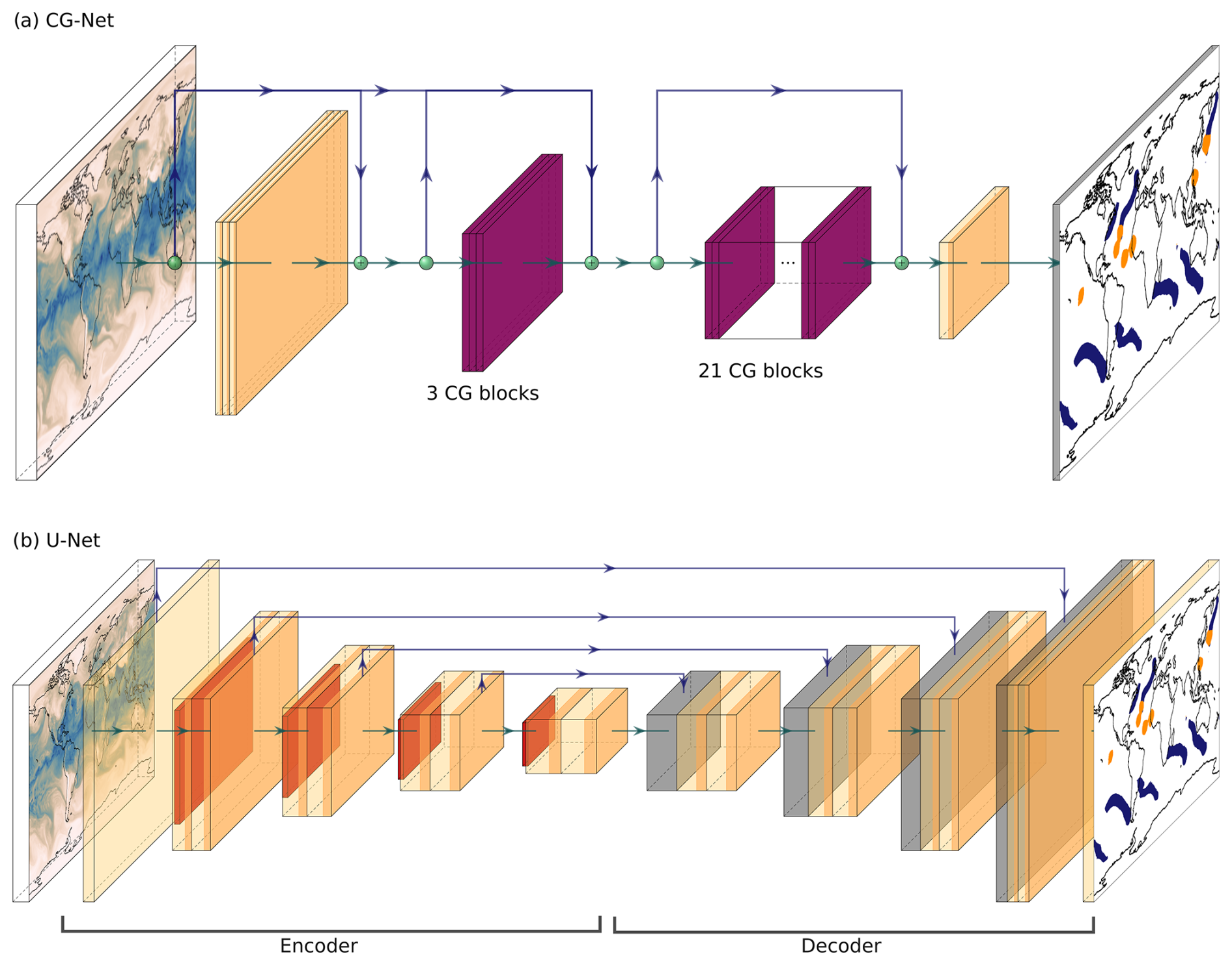
Figure 1 Schematic illustration of the (a) CGNet (Wu et al., 2021) and (b) U-Net (Ronneberger et al., 2015) CNN architectures. Yellow color denotes convolutional layers, red average pooling layers, blue/grey transposed convolutional layers, and violet context guided blocks. Blue arrows indicate skip connections.

We use the same CGNet configuration used by KS20, who in turn followed Wu et al. (2021). Our U-Net configuration is based on Ronneberger et al. (2015). For training CGNet and U-Net, we follow KS20. Most grid points in the ClimateNet dataset belong to the background class; hence an imbalance exists between the frequency of the three classes. KS20 use the Jaccard loss function beneficial in cases of class imbalance (Rahman and Wang, 2016). It applies the intersection-over-union (IoU; Everingham et al., 2010) metric commonly used in semantic segmentation (e.g., Cordts et al., 2016; Zhou et al., 2017; Abu Alhaija et al., 2018). The IoU score characterizes the overlap of two features by dividing the size (in the computer vision literature as number of pixels, in our case in grid points) of feature intersection by the size of the feature union.³ If two features are identical, the IoU score equals 1; if they do not overlap at all, the score equals 0. The Jaccard loss function is minimized (equivalent to maximizing IoU) using the Adam optimizer (Kingma and Ba, 2015), with a learning rate of 0.001. Since random weight initialization leads to differing results in different training runs (Narkhede et al., 2022), we train each network five times and select the best performing. We use convolution kernels of size 3×3 grid points. Grid boundaries in longitudinal direction are handled with circular (i.e., cyclic) padding; at the poles, replicate padding is used.

KS20, as well as P21, only uses a subset of the 16 variables contained in the ClimateNet dataset: TMQ, U850, V850, and PSL in KS20 and TMQ, U850, V850, and PRECT in P21. We reproduce the KS20 CGNet setup for our objective of investigating whether it bases its detection on plausible patterns. For evaluation, IoU scores are computed for each feature class individually and for comparison with values provided by KS20 as multiclass means. All scores are computed for the test data (cf. Sect. 2) and listed in percent.

Table 2 Intersection-over-union scores reached by CGNet trained as proposed by KS20, using a batch size of 4 and 10. For comparison, scores for U-Net are provided. All values are computed for the test data and are listed in percentages. The highest score per column is written in bold.

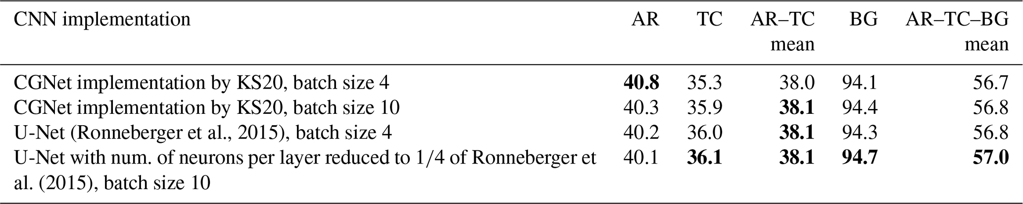
Table 2 lists evaluation results for both CGNet and U-Net. KS20 only provide an evaluation score for the AR–TC–BG mean of 56.1 %. Our reproduction (using the same implementation) yields a similar score (slightly different due to random initialization); Table 2 in addition shows the scores for the individual feature classes. KS20 use a training batch size of 4; with 20 training-evaluation epochs a single training run takes about 19 min on an 18-core Intel Xeon^® Gold 6238R CPU with 128 GB RAM and a Nvidia A6000 GPU with 48 GB VRAM. To speed up training, the batch size can be increased. For instance, a batch size of 10 reduces training time for a single run by 10 % without significantly deviating from the evaluation results. The U-Net implementation achieves similar scores, confirming that the detection task can be learned by different CNN architectures. Also, our experiments showed that for U-Net, reducing the number of neurons per layer to one-quarter compared to the original Ronneberger et al. (2015) implementation reduces training time by 35 % without significantly deviating from the evaluation results. One may hypothesize that due to its larger number of weights the U-Net architecture has an increased potential to learn complex tasks and thus may achieve higher IoU scores for the problem at hand. This, however, seems not to be the case. Also, U-Net in our case requires 50 training-evaluation epochs to converge, requiring about 46 min on our system.

Concluding, all CNN setups achieve very similar evaluation scores, which provides confidence that they are learning similar structures that can be further analyzed using LRP.

We note that the size of the ClimateNet dataset (cf. Sect. 2) can be considered small for training a deep CNN, a challenge also encountered, e.g., in the literature for medical image segmentation (e.g., Rueckert and Schnabel, 2020; Avberšek and Repovš, 2022). P21 stated they expect CNN performance to improve if a larger dataset was available. However, we also note that ClimateNet's characteristics of containing differing labels by multiple experts for many time steps may be effective in avoiding overfitting. Also, it may limit achievable IoU scores. If strong overfitting was present, we expect physically implausible structures to show up in the LRP results. Also, strong overfitting typically results in evaluation scores being distinctly better for the training data compared to the test data (e.g., Bishop, 2007). For example, for the CGNet implementation by KS20, batch size 10, we obtain the following IoU scores for the training data: AR = 43.6 %, TC = 37.7 %, BG = 95.2 %, and AR–TC–BG mean = 58.8 %. These scores are very close to those listed in Table 2 for the test data, indicating that no overfitting is present. In comparison, if we deliberately overfit CGNet by training with 100 training-evaluation epochs (instead of 20), we obtain IoU scores of AR = 60.0 %, TC = 53.3 %, BG = 96.7 %, and AR–TC–BG mean = 70.0 % for the training data and AR = 37.8 %, TC = 32.5 %, BG = 94.4 %, and AR–TC–BG mean = 55.0 % for the test data.

4 Adapting LRP to semantic segmentation

For our first objective, we adapt LRP to the semantic segmentation task. LRP was originally developed to understand the decision-making process of ANNs designed for solving classification tasks (Bach et al., 2015). After a classification ANN has computed class probabilities from some input data grid, LRP considers a single feature class by only retaining its probability (all other class probabilities are set to zero). This modified output is interpreted as the initial value for the relevance to be computed; it is propagated backwards through the network towards the input layer. Figure 2 illustrates the approach. In an iterative process, the relevance $R_{l+\mathrm{1},m}$ of a given neuron m in a network layer l+1 is distributed over all neurons n in the preceding layer l (conserving the total relevance). Practically, this is implemented by iteratively computing the relevance R_l,n of the neurons in layer l, as proposed by Montavon et al. (2019):

$$\begin{array}{}\text{(1)}& R_{l,n}={\sum }_m{\displaystyle \frac{a_{l,n}\cdot \mathit{\rho }\left(w_{l,n}^{\left(l+\mathrm{1}\right),m}\right)}{\mathit{ϵ}+{\sum }_n{a}_{l,n}\cdot \mathit{\rho }\left(w_{l,n}^{\left(l+\mathrm{1}\right),m}\right)}}{R}_{l+\mathrm{1},m}.\end{array}$$

Here, a_l,n denotes the activation value of neuron n, $w_{l,n}^{\left(l+\mathrm{1}\right),m}$ the weights between neurons n and m, ρ an optional function that modulates the weights, and ϵ a constant value that can be used to absorb weak or contradictory relevance. Note that in our case, activation a and relevance R are 3-D grids. Their size is given by the size of the 2-D data grid of the respective layer times the number of classes. The weights w can be scalars or convolution kernels depending on layer type. We refer to Montavon et al. (2019) for further details. In this study, we use the so-called LRP_z rule (M22; also called LRP-0 rule; e.g., Montavon et al., 2019). That is, the function ρ is a simple identity mapping, and ϵ equals $\mathrm{1}\times {\mathrm{10}}^{-\mathrm{9}}$ to prevent division by zero. The relevance distribution of the input layer is the desired result. LRP_z distinguishes between positive and negative contributions. They can be interpreted as arguments for (positive relevance) and against (negative relevance) classifying grid points as belonging to a feature.

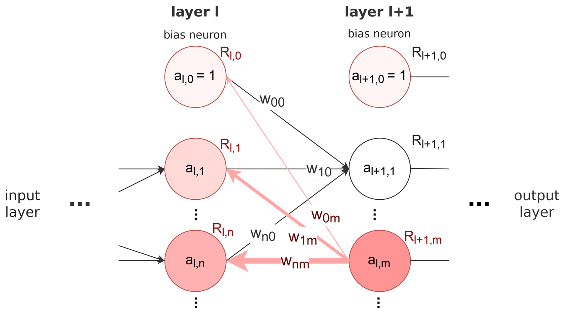
Figure 2 Schematic illustration of two (hidden) layers of an ANN (cf. Eq. 1). a_l,m denotes the activation of neuron m in layer l, R_l,m the corresponding relevance, and w_n,m the weight between neuron n and m. Neuron “0” of each layer is a bias neuron. Red color intensity symbolizes exemplary relevance back-propagated from neuron m in layer l+1 towards layer l, distributed according to neuron activation and weights. In setups discussed in this study, activation a and relevance R are 3-D grids with size of the current layer-dependent horizontal grid times the number of classes; the weights w can be scalars or convolution kernels depending on layer type.

Other LRP rules exist, and M22 discussed their properties for CNN architectures designed for classification (note that the LRP_comp and LRP${}_{\mathrm{comp}/\mathrm{flat}}$ rules recommended by M22 are not directly applicable to our setup; e.g., our CNNs do not contain fully connected layers, and also, the LRP${}_{\mathrm{comp}/\mathrm{flat}}$ rule cannot distinguish between different input variables).

As noted in Sect. 2, LRP using the LRP_z rule suffers from what is referred to by M22 as the “ignorant-to-zero-input issue”. An ANN's bias neurons (e.g., Bishop, 2007; index 0 in each layer in Fig. 2) are required, e.g., to consider input values close to zero that would otherwise have no effect on the ANN output due to the multiplicative operations at each neuron (e.g., Saitoh, 2021). Due to the design of LRP_z, relevance assigned to bias neurons is not passed on to the previous layer and will not be included in the final result. Hence, input values of zero will receive zero relevance (Montavon et al., 2019).

For our setup we note that, in contrast to the ANNs used by M22, CGNet and U-Net as used in the present study contain batch normalization layers (Ioffe and Szegedy, 2015). These layers apply z-score normalization to the output of the convolutional layers. Additionally, the normalized values are shifted and rescaled according to two learned parameters β and γ. This normalization cancels the bias effect. It is, however, subsumed by β and still present. In practical implementations, the bias neurons and weights are hence deactivated during training (Ioffe and Szegedy, 2015). This becomes relevant for the computation of relevance, which can be done separately for convolutional layers (Bach et al., 2015) and batch normalization layers (Hui and Binder, 2019). Alternatively, implementations have been proposed in which both layers are merged, with the advantage that relevance only needs to be computed for the merged layer (Guillemot et al., 2020). In our work, relevance needs to be computed many times for a given ANN (for grid points and features). For efficiency we choose the second option, as a merged layer only needs to be computed once. The merged layer weights are inferred from the original two layers. In particular, the bias weights are reintroduced, and the ignorant-to-zero issue persists as in M22.

LRP implementations for classification tasks have been described in the literature (e.g., Montavon et al., 2019; M22). For semantic segmentation tasks, the question arises of how the gridded output (instead of single class probabilities) should be considered. A straightforward approach is to consider an individual detected feature (i.e., a region of connected grid points of the same class) and to compute a relevance map for each grid point of the feature, i.e., treating each grid point as an individual classification task. Then, the resulting relevance maps can be summed to obtain a total feature relevance. While for a given location the contribution from different relevance maps can be of opposite sign, the sum expresses the predominant signal. For more detailed analysis, positive and negative relevance can be split into separate maps. Also, we propose to compute the extent to which different grid points of a feature contribute to the (total or positive or negative) relevance in a selected region R. The resulting maps show, for each grid point of a feature, the summed relevance that this point has contributed to all grid points in R.

An important aspect is that the absolute relevance values computed by LRP depend on the absolute probability values computed by the CNN. For example, if a grid point is classified as a TC based on probabilities (TC = 0.3, AR = 0.2, BG = 0.1), the corresponding relevance map will contain lower absolute relevance values than if the probabilities were, e.g., TC = 0.8, AR = 0.6, and BG = 0.4. The question arises of whether the relevance values should be normalized before summation, as the absolute probability values are not relevant for assigning a grid point to a particular class. They can, however, be interpreted as how “likely” the CNN is in assigning a class to a certain grid point. This aligns with Montavon et al. (2019), who link the ANN output with the probability of each predicted class. We hence argue that for all grid points belonging to a given feature, no normalization should be applied. This way, in the resulting total relevance map, the individual grid points' contributions are weighted according to their probability of belonging to the feature; higher relevance is deemed to be more important for the overall feature as well.

To compare relevance maps of distinct features, or to jointly display the relevance of multiple features in a single map, we however argue that the relevance maps of the individual features should be normalized first. This ensures that the spatial structures relevant for the detection of a feature show up at similar relevance magnitudes.

For computing relevance maps for the individual grid points, an existing LRP implementation for classification, e.g., Captum (Kokhlikyan et al., 2020), can be used by adding an additional layer to the network that reduces the output grid to a single point (this corresponds to setting the output probabilities of all grid points except the considered one to zero). This approach has recently been used by Farokhmanesh et al. (2023) for an image-to-image task similar to semantic segmentation. The resulting relevance maps can be summed and normalized in a subsequent step. Depending on grid size and number of neurons in the CNN, this approach, however, can be time-consuming (in our setup, a single LRP pass requires about 100 ms; with an AR feature typically consisting of more than 5000 grid points in the given dataset, calculating LRP with this approach sums to about 8 min for an AR feature). To speed up the computation, we modify the approach by retaining the output probabilities of all grid points that belong to a specific feature. The LRP algorithm is executed only once (thus only requiring about 100 ms for an entire AR feature). Due to the distributive law for addition and multiplication, this is equivalent to the first approach. This approach has also been used by Ahmed and Ali (2021) for a specific U-Net architecture in a medical application, although for the entire data domain instead of individual features.

To apply LRP with the CGNet architecture, the additional challenge of handling CGNet-specific layer types arises. In addition to layer types also present in the U-Net architecture (for which LRP implementations have been described in the literature, including convolutional layers (Montavon et al., 2019), pooling layers (Montavon et al., 2019), batch normalization layers (Hui and Binder, 2019; Guillemot et al., 2020), and concatenation-based skip connections (Ahmed and Ali, 2021)), CGNet uses addition-based skip connections, a spatial upscaling layer, and a global context extractor (GCE; Wu et al., 2021).

For addition-based skip connections, we first calculate the relative activations of both the skip connection and the direct connection in relation to the summed activation. Next, the relevance of the subsequent deeper layer is multiplied by these relative activations to determine the relevance for both connections. LRP for spatial upscaling layers is calculated by spatially downscaling the relevance maps by the corresponding scaling factor. Following the argumentation by Arras et al. (2017) for adapting LRP to multiplicative gates in long short-term memory (LSTM) units, we omit the relevance calculation of GCE units.

5 Case study: plausibility of spatial relevance patterns for detected TC and AR features

For our second objective, we discuss the example of the time step labeled “27 September 2013”. We assess the plausibility of spatial relevance patterns obtained using our adapted LRP approach and the CGNet setup that reproduces the KS20 setup (using z-score normalization; cf. Table 2). In the chosen example, several TC and AR features were present that we consider representative.

Figure 3a and b show global maps of TMQ and PSL of the chosen time step, overlaid with expert-labeled and CNN-detected TC and AR features. Distinct features in the North Atlantic region are enlarged. In general, TCs are characterized by high humidity and minima in PSL (e.g., Stull, 2017) and ARs by strong horizontal moisture transport (implying high humidity and wind speed; e.g., Ahrens et al., 2012). ARs also take the form of elongated bands of elevated humidity connected to mid-latitude cyclones (Gimeno et al., 2014). These aspects are commonly used by rule-based detection methods (e.g., Tory et al., 2013; Shields et al., 2018; Nellikkattil et al., 2023); we are hence interested in whether CGNet learns similar aspects.

In addition, Fig. 3c and d show the z-score-normalized TMQ and PSL fields that are the actual input to the ANN. As discussed in Sect. 4, the employed LRP_z rule is “ignorant to zero input” (M22), it is hence important to see where zero values are input to the CNN.

Figure 3e and f show the relevance of TMQ and PSL for the detected TC features (i.e., the summed relevance of all grid points classified as TC as described in Sect. 4). We interpret the relevance maps as “what the CNN looks at” to detect a feature and where it collects arguments for (positive relevance) and against (negative relevance) classifying grid points as belonging to a feature. If the relevance is close to zero despite having a non-zero input value, the corresponding location is considered irrelevant to the current feature of interest.

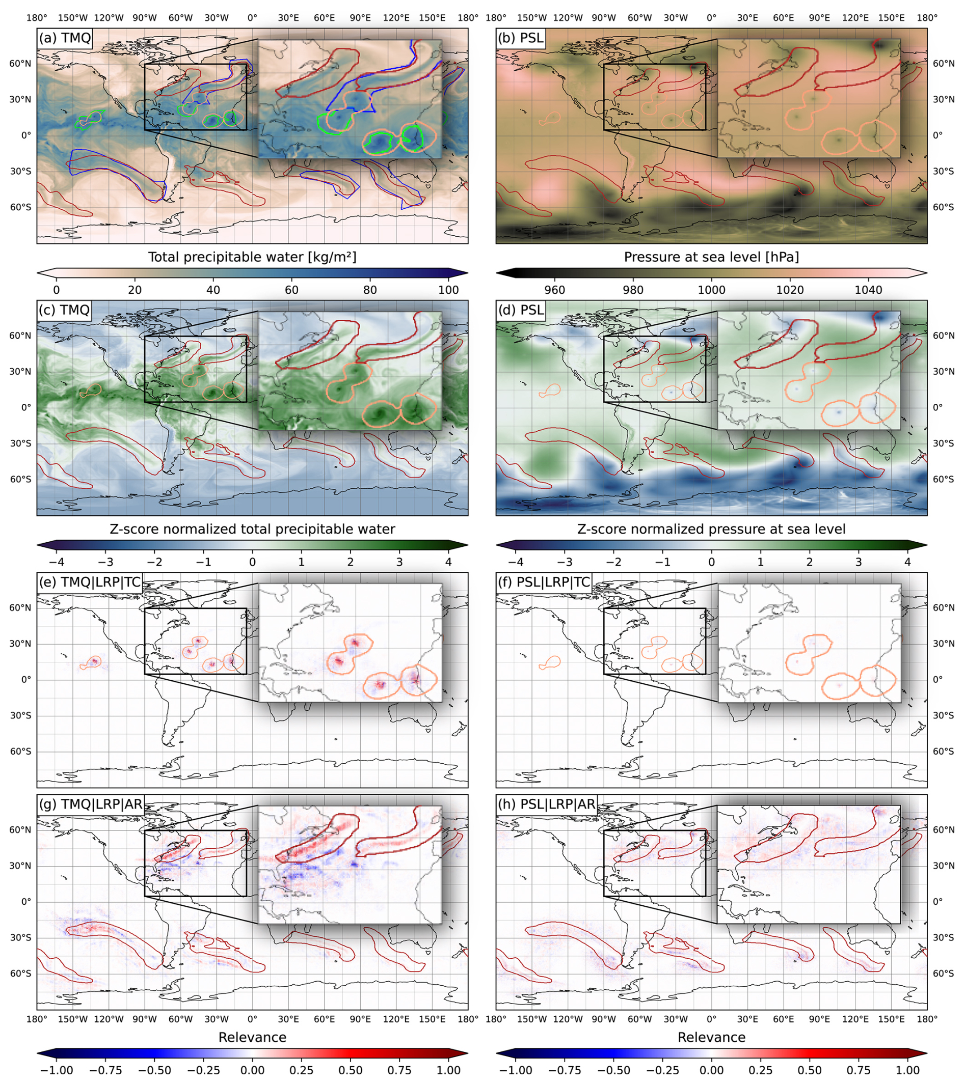
Figure 3 Global maps of (a) TMQ and (b) PSL for the time step contained for 27 September 2013 in the ClimateNet dataset. Orange (red) contours show TC (AR) features detected with CGNet using the KS20 setup. Green (blue) contours show TC (AR) features labeled by an expert. Panels (c) and (d) show z-score-normalized fields input to the ANN. Panels (e) and (f) show summed TMQ and PSL relevance of all grid points classified as TC and panels (g) and (f) the summed relevance of all grid points classified as AR.

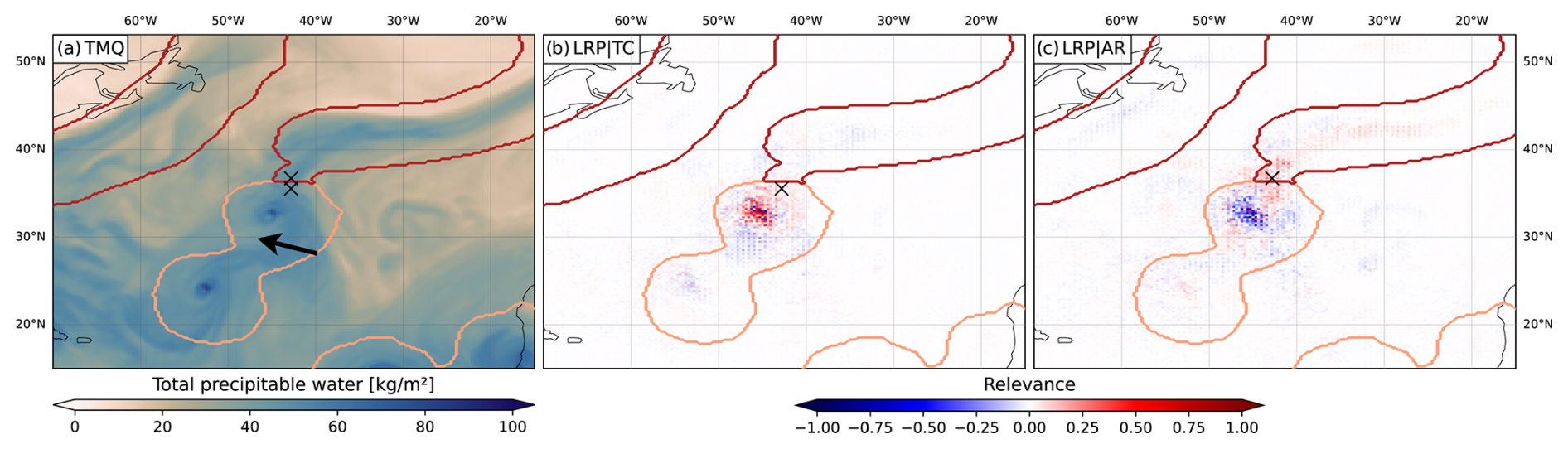
Figure 4 (a) Close-up of TMQ as shown in Fig. 3a for the North Atlantic region. Black “x” mark two selected single grid points, the southern one within the TC feature and the northern one within the AR. (b) TMQ relevance for the southern (TC) grid point. (c) TMQ relevance for the northern (AR) grid point.

For both TMQ and PSL, CGNet learns to positively consider extreme values at the center of the detected TCs, with TMQ considered more relevant than PSL (normalized relevance of up to 1.0 vs. up to 0.5). The relevance mostly is spatially confined to the feature region. Positive TMQ relevance is mostly found at TMQ maxima, which also correspond to z-score-normalized maxima (Fig. 3a and c). PSL relevance is also collocated with PSL minima, which, however, are surrounded by bands of close-to-zero values after z-score normalization. We hypothesize that this can cause the lower relevance values compared to TMQ. That is, CGNet could consider PSL values more strongly, but this is not discernible in the LRP_z-computed relevance of the used setup.

A further noticeable characteristic in Fig. 3e and f is that the detected TC features are markedly larger than the relevant regions. Here our hypothesis is that CGNet learned to classify grid points at a certain distance around point-like extrema as TC. That is, for grid points at the edge of a feature, the most relevant information is that it is at a specific distance to the TMQ maximum and PSL minimum. This hypothesis would be consistent with the specific capabilities of CNNs; their convolution filters take neighboring grid points into account (e.g., Bishop, 2007). If CGNet had primarily learned some sort of thresholding on TMQ or PSL, and no information about the spatial structure of the fields, we would have expected the relevance to cover the feature area (with values above/below a specific threshold) more uniformly.

To test the hypothesis, we consider two individual grid points in the inset region in Fig. 3 that are of interest because they are close to the border of the TC and AR features around 45° W and 35° N: how does CGNet distinguish between the two feature classes in this region? Figure 4 shows TMQ relevance maps for the two points, the southern one being classified as belonging to the TC and the northern one as belonging to the AR (black crosses in Fig. 4a; note that in Fig. 4b and c the relevance for the classification of the single grid points only is shown, not the summed relevance of all feature grid points as in Fig. 3). For the TC grid point, Fig. 4b shows that the CNN considers the nearby TMQ maximum at 43° W and 31° N as a strong argument for its decision to classify the point as TC, confirming our hypothesis. Some patches, in particular south of the TC center, are considered arguments against, though at much weaker relevance magnitude. We hypothesize that this may be due to the shape of the TMQ field in this region with weak filaments of TMQ being drawn into the TC from the southwest (arrow in Fig. 4a). We will come back to this issue in the next section. For the AR grid point, CGNet considers the nearby TMQ maximum as a strong argument against classifying the point as AR. In contrast, the also nearby band of high TMQ extending from 40° W and 40° N towards the northeast is considered an argument for the point being part of an AR. We interpret these findings such that the CNN indeed considers the spatial distance to a point-like TMQ maximum and possibly also the filamentary structures in TMQ. Note that the final classification decision, however, is of course based on all input fields.

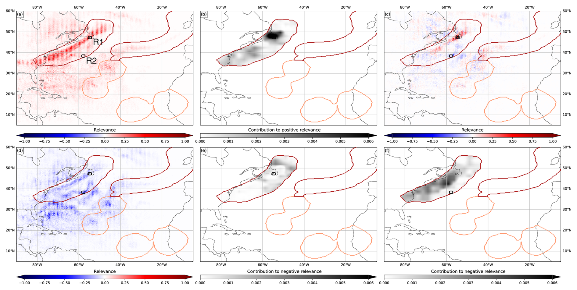
Figure 5 Same as the inset in Fig. 3g but showing (a) only the positive component of total TMQ relevance, (b) parts of the AR that contributed to positive TMQ relevance in region R1, (c) TMQ relevance for classifying the grid point marked with X as AR, (d) only the negative component of total TMQ relevance, (e) parts of the AR that contributed to negative TMQ relevance in R1, and (f) the same as (e) but for R2.

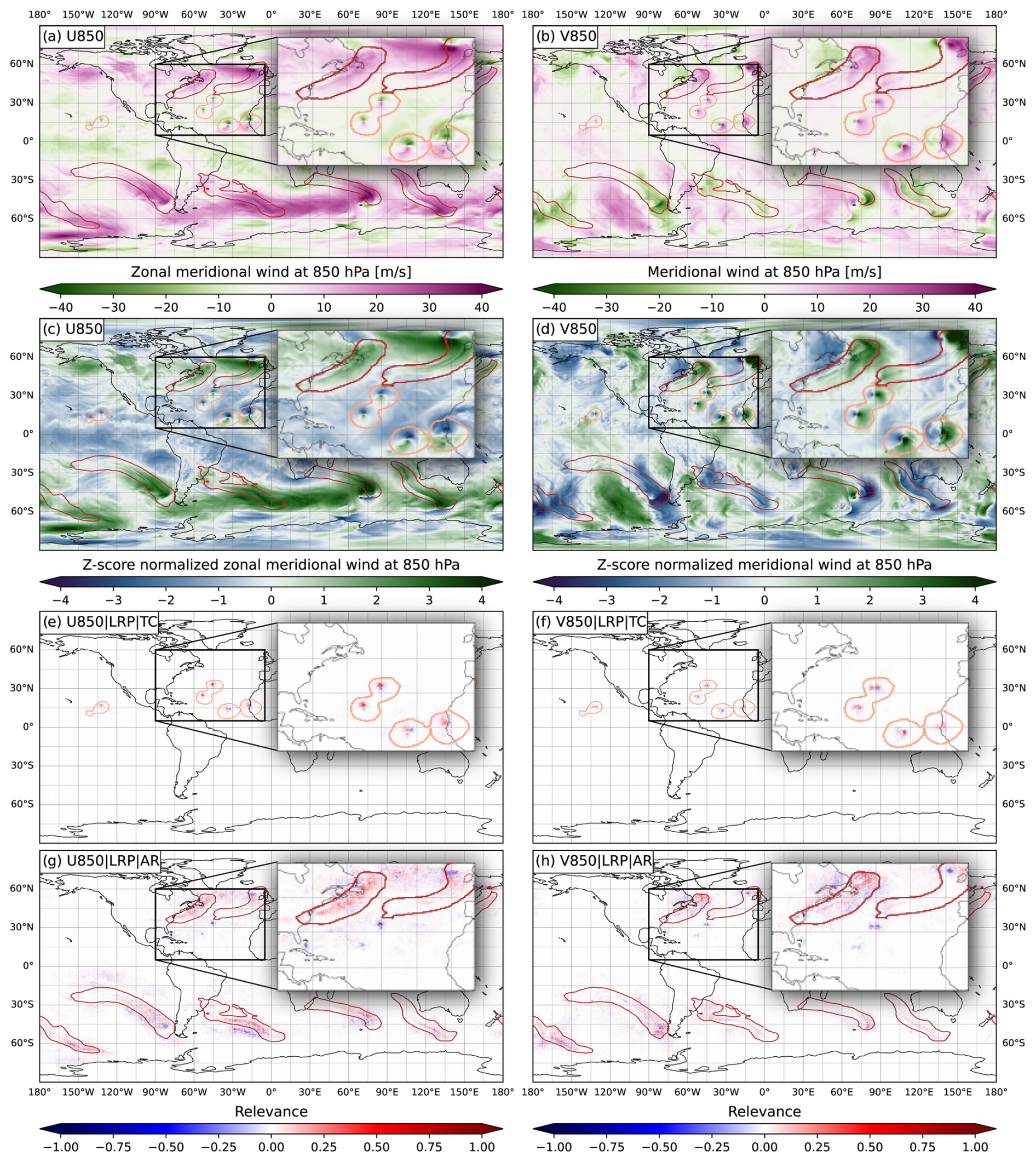
Figure 6 Same as Fig. 3 but for (left column) zonal wind at 850 hPa and (right column) meridional wind at 850 hPa.

Figure 3g and h show the relevance of TMQ and PSL for the detected AR features. We again focus on the North Atlantic region in the inset, containing two ARs. The elongated band of high TMQ associated with the eastern AR is surrounded by drier air, making it distinctly stand out in Fig. 3a. CGNet finds positive relevance in this band; few arguments against the structure being an AR are found in its surroundings except for the discussed TMQ maximum in the TC directly south of the AR (Fig. 3g). However, again we note that if information directly around the band of high TMQ were considered by the CNN, it would not show up in the relevance map as the z-score-normalized values surrounding the band are close to zero (Fig. 3c).

The western AR, however, is not as clearly surrounded by drier air and hence not as clearly discernible in the TMQ field (Fig. 3a). While for this feature also the elongated band of high humidity is taken as an argument for the AR class, at the southern edge and south of the AR, regions of arguments against show up (Fig. 3g). We interpret this as some sort of uncertainty of the CNN, like a human expert that would analyze the region around this AR more carefully, also considering other available variables to make their decision.

The western AR also is interesting as it is not among the expert labels (Fig. 3a), although we note that the discussed time step has been labeled by a single expert only (cf. Sect. 2). Is this a “false positive” or did the expert miss a potential AR? To further understand CGNet's reasoning, we split the total TMQ relevance into positive and negative components. Also, for selected regions, we investigate which parts of the AR contributed to the relevance (cf. Sect. 4).

Figure 5a shows that for some of the grid points that comprise the AR, the regions of high TMQ at the southern edge and south of the AR are also taken as (weak) arguments for belonging to the AR. Figure 5d shows that for some grid points the elongated band of high TMQ inside the AR is taken as an argument against. Further analysis shows that the predominantly positive relevance along the elongated band is mostly caused by grid points on or close to the band. As an example, Fig. 5b shows that positive relevance in a selected region R1 is mostly caused by grid points inside and around R1. Individually, these grid points show relevance patterns as shown in Fig. 5c. Here, with respect to TMQ, the elongated band is the main argument for belonging to the AR. Figure 5e shows that negative relevance in R1 is mostly caused by grid points at a certain distance to R1, with a distinct “blocky” shape that we attribute to the CNN's convolutional layers. We interpret this as CGNet having learned that (1) grid points located on or close to an elongated band of high TMQ likely belong to an AR, and (2) grid points located at some distance to such a structure likely do not belong to an AR. Figure 5f confirms this hypothesis. R2 is located on another filament of high TMQ close to but separate from the AR's “main band” of high TMQ. Negative relevance in R2 is mostly caused by grid points on the AR's “main band”. For these grid points, being close to another band-like structure of high TMQ seems to be an argument against belonging to an AR.

We provide a more complete picture in Figs. S6 and S7 in the Supplement, showing relevance contribution for further regions. For many grid points in the discussed feature, the presence of the band-like structures of high TMQ at the southern edge and south of the AR counter the arguments of the “main band” for an AR and hence cause “uncertainty”. We argue, however, that this behavior of the CNN is plausible and that a human expert could also have labeled the structure as an AR.

Figure 3h shows that for AR detection CGNet cannot infer much information from the PSL field. While it “looked” at the regions surrounding the ARs, the relevance field is weak and noisy, and no recognizable structure is found. This is plausible since in Fig. 3b there are no discernible PSL structures visible for the AR features. To the best of our knowledge, there are also no rule-based systems that use PSL for AR detection.

Figure 6 shows, however, that both 850 hPa wind components are used for the detection of both TCs and ARs. The western AR in the inset is characterized by high zonal wind (Fig. 6a). It coincides with a clearly positively relevant structure (Fig. 6g). Meridional winds are strongest around the mid-latitude cyclone at the northern end of the AR (Fig. 6b). CGNet also considers this as positively relevant (Fig. 6h). The dipole structure discernible in both wind components close to cyclone centers (both tropical and mid-latitude) is considered an argument against ARs by the CNN (negative relevance in Fig. 6g and h). Our interpretation is that CGNet learned to identify such dipoles with TCs and cannot infer that a mid-latitude dipole northeast of an AR would be an argument for the AR feature. This is supported by that for detection of TC features, the dipoles are considered positively relevant (Fig. 6e and f). Both wind components are also widely used in rule-based detection systems, for example by three of the four algorithms discussed by Bourdin et al. (2022) for detection of TCs. For rule-based AR detection, wind components are contained in the integrated vapor transport (IVT) variable that is commonly used (Shields et al., 2018; Wick et al., 2013).

We conclude the discussion with the interpretation that CGNet in the present setup learned overall very plausible structures to detect TCs and ARs, which is very promising for gaining confidence in CNN-based detection of atmospheric features.

Reproductions of Figs. 3 and 6 when using U-Net instead of CGNet are provided in the Supplement (Figs. S8 and S9). Despite the differences in CNN architecture (cf. Sect. 3), very similar results are found. Notable differences include that the U-Net setup detects smoother feature contours and that its relevance values are more pronounced and show smoother spatial patterns. We consider it promising, however, that two different CNN architectures learn very similar patterns.

6 Relevant input variable values: the issues of shape and input normalization for explaining feature detection

Figures 3 to 6 show a single time step that we consider representative as an example of the spatial relevance patterns obtained from LRP. For a more complete picture of what the CGNet has learned, we are interested in statistical summaries of input values that it considers relevant. The goal is to see if, for example, also on average high values of TMQ are learned to be most relevant for TC and AR detection.

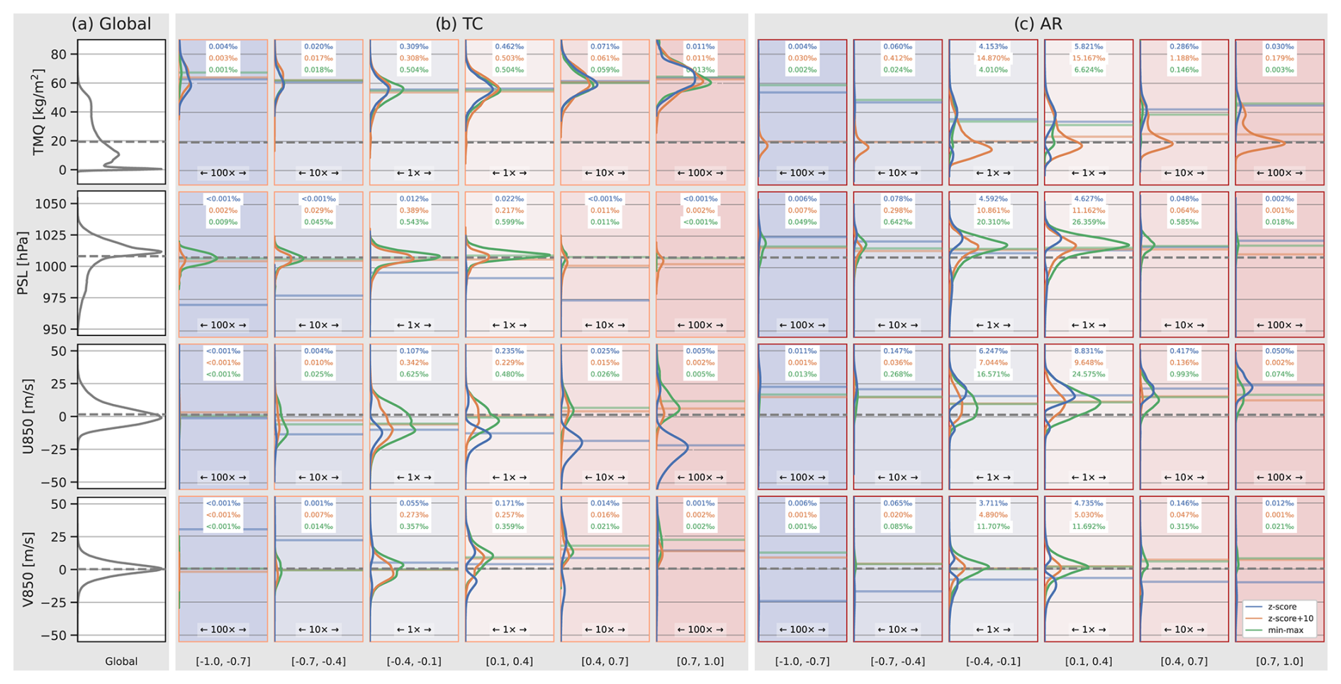
Figure 7 Distributions of CGNet input variable values in the test dataset. (a) Global distribution (all grid points). Dashed horizontal lines show distribution means, for reference also shown in the other panels. (b) Distributions of grid points with relevance magnitude > 0.1 for TC detection, at six different relevance ranges. The range [−0.1…0.1] is omitted. Shown are distributions for z-score-normalized input values (blue curves), shifted z-score normalization (orange), and min–max normalization (green). Horizontal lines show distribution means. The numbers at the top of each box denote fraction (in ‰) of grid points in the corresponding relevance range. Note the horizontal scaling: since much fewer grid points are assigned high relevance values, to see the shape of the distributions we horizontally scale the relevance range [0.4…0.7] 10 times and the range [0.7…1.0] 100 times compared to the range [0.1…0.4]. (c) Same as (b) but for AR detection.

We compute distributions over all time steps in the test dataset (cf. Sect. 2) of the CNN input variables, both at all grid points and at grid points considered relevant to different extent (note that, as seen in Figs. 3 and 6, this includes grid points outside the detected features). Figure 7 shows the distributions of TMQ, PSL, U850, and V850. As reference, the value distributions for the entire globe, i.e., all grid points, are shown (Fig. 7a). To learn which variable values are considered relevant by LRP for TC and AR detection, we divide the relevance range [−1…1] into six distinct intervals of width 0.3 and show distributions for each feature and interval. The relevance range [−0.1…0.1] is omitted to mask out regions of zero and low relevance. Note that for all variables, this includes over 98 % of all grid points. That is, on average fewer than 1 % of all grid points are assigned relevance values with magnitude larger than 0.1 in the present CGNet setup. Distributions of the relevance range [−0.1…0.1] hence look very similar to the reference distributions of the entire globe.

First notice that CGNet for TC detection, also averaged over the entire test dataset, considers high values of TMQ positively relevant. Already for the relevance range [0.1…0.4], the distribution peaks at values slightly above 55 kg m⁻², which is at the upper end of the global distribution. The TMQ distributions of grid points with higher relevance peak at even slightly higher values (although much fewer grid points are assigned high relevance). This finding is in line with our hypothesis from Sect. 5 that CGNet learned to associate TCs with TMQ extrema.

It is noticeable that the distributions of positive and negative relevance intervals cover similar TMQ values, however, with more relevant grid points on the positive side. This raises the question of why similar values are considered in both pro and contra arguments – GG-Net could have also learned to use low TMQ values as an argument against a TC feature. However, high TMQ values occur not only within TCs but also elsewhere particularly in the tropics (cf. Fig. 3a). In Sect. 5 we discussed that CGNet is capable of learning spatial structure by means of convolution filters. We hence hypothesize that the “pro/contra TC decision” is based on spatial structure, which cannot be inferred from the relevance distributions in Fig. 7.

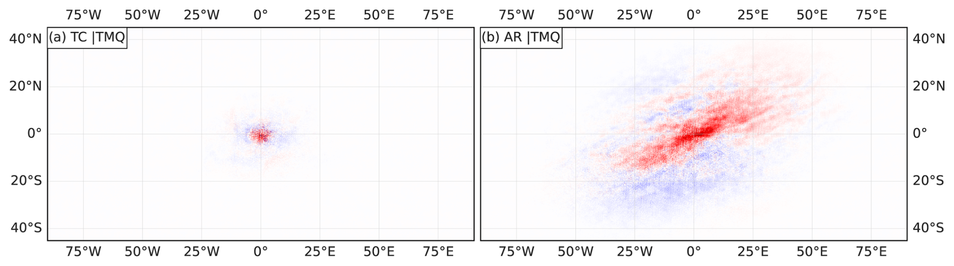
Figure 8 Composite relevance maps for TMQ, averaged over (a) all TC features in the test dataset and centered on the features. (b) The same for ARs. For clarity of presentation, only AR features from the Northern Hemisphere are composited due to the difference in orientation on the Southern Hemisphere.

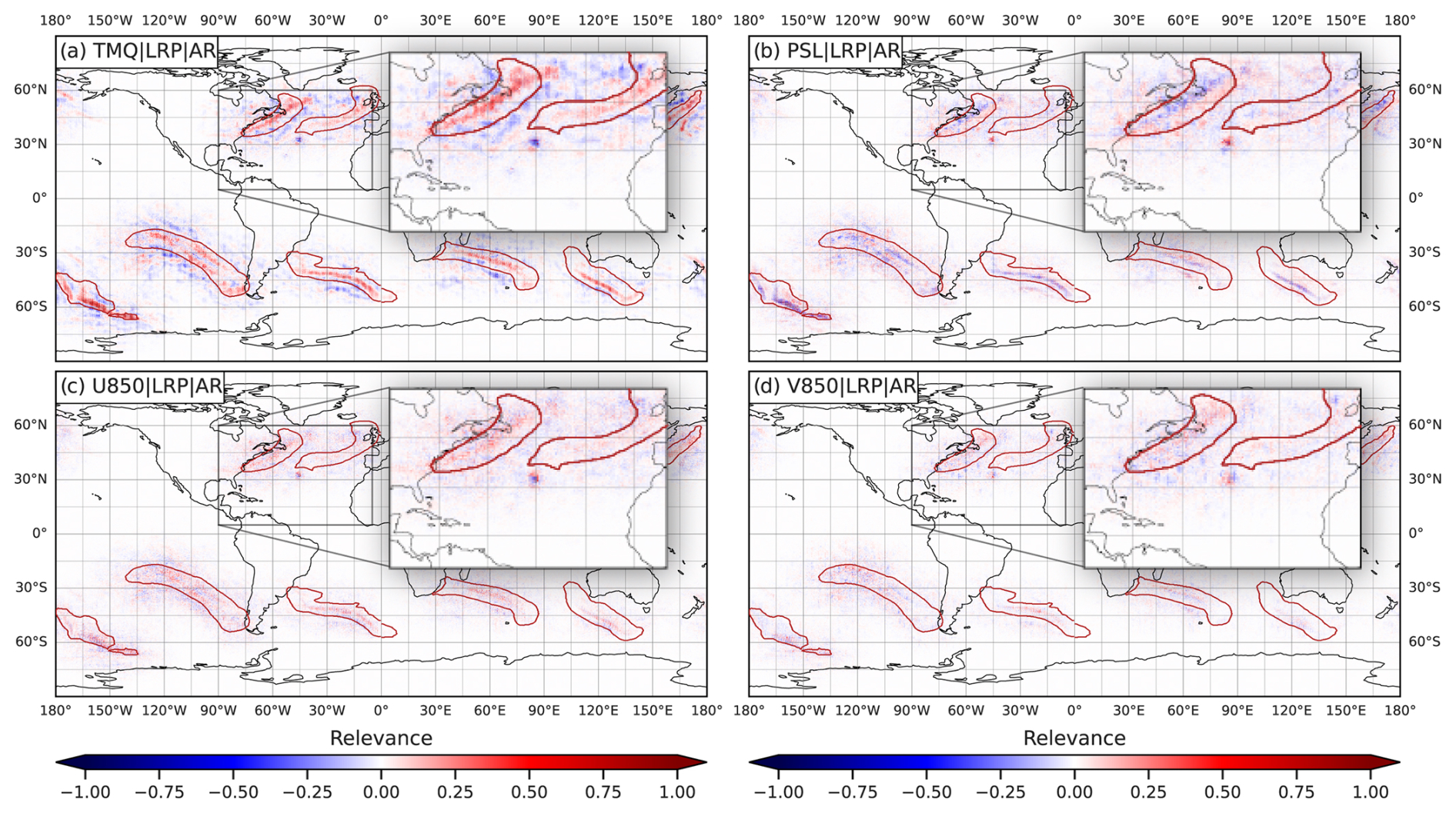
Figure 9 Same as Figs. 3g and h and 6g and h but for relevance obtained from CGNet trained with z-score-normalized input data shifted by +10.

First consider the distributions shown with the blue curves in Fig. 7b. They correspond to the KS20 setup with z-score-normalized data used in the previous sections. Most distributions of relevant grid points clearly differ from the global reference distributions; hence CGNet gathers information from the values of the input variables.

To investigate, we compute composite relevance maps of all TC and AR features in the test dataset. Figure 8 shows the average relevance of TMQ for both feature classes, obtained by averaging the relevance of all features. For clarity of presentation, only AR features from the Northern Hemisphere are considered since their orientation differs between both hemispheres (if ARs from both hemispheres are plotted, we obtain a cross-shaped pattern). Figure 8 shows that for TCs, CGNet on average learned to detect spherical structures. For ARs, elongated structures from the southwest to northeast are detected (northwest to southeast on the Southern Hemisphere; not shown). We interpret this finding as strong support for the hypothesis that spatial structure plays a crucial role in the detection process. However, we note that more detailed investigation is required. Shape information is not directly accessible via LRP. To the best of our knowledge, also in general not much of the literature has investigated the explanation of shapes in CNN-based feature detection. While recently a potentially useful method (Concept Relevance Propagation, CRP; Achtibat et al., 2023) has been published, it has yet to be applied to meteorological data and is left for future work.

Figure 7c shows the TMQ distributions of grid points relevant for AR detection. While the distributions also show that more relevant grid points correspond to higher TMQ values (which is plausible given the discussion in Sect. 5), here we observe bimodal distributions with minima located around the mean of the global distribution. As discussed in Sects. 4 and 5, values around the global mean become close to zero after z-score normalization. Hence, the minimum could be a consequence of the “ignorant-to-zero-input issue” (M22). The question hence arises of whether CGNet indeed does not consider TMQ values around the global mean of 19.3 kg m⁻² (cf. Table 1; for which to the best of our knowledge there would be no plausible physical reason) or whether that relevance information is simply missing in LRP_z output.

To investigate, we retrain CGNet with two alternative normalizations. First, we shift the z-score-normalized data by +10. The value of 10 is chosen as minimum values after z-score normalization are about −8; hence the shift ensures that all input data are positive and at some distance from zero. Second, we apply the min–max normalization (e.g., García et al., 2014) that linearly scales all inputs to the range [0…1]. It, however, has the disadvantage of being more sensitive to outliers and cannot ensure that all inputs are treated equally important by the CNN (since the means of the different input variables are not mapped to the same normalized value; cf. Sect. 2).

IoU evaluation scores for both alternative normalizations are comparable to the original z-score normalization (e.g., AR–TC mean of 37.8 for z score+10 and 37.7 for min–max, compared to 38.1 for the original z-score setup). Also, Fig. 7c clearly shows that with the alternative normalizations, TMQ values around the global mean are attributed to be relevant. The minimum in the z-score-normalization distribution vanishes, and in particular for the z-score+10 data, a maximum is found instead. Hence, CGNet does consider TMQ values in this range relevant.

Figure 9 revisits the case from Sect. 5 and shows AR relevance maps obtained from the CGNet trained with z-score+10-normalized inputs. Full reproductions of Figs. 3 and 6 for both alternative normalizations are provided in the Supplement (Figs. S2–S5). Figure 9a shows that, compared to Fig. 3g, the elongated AR bands of high TMQ are still distinctly positively relevant. However, some noisy relevance is now found in the surroundings of the ARs, exactly where TMQ values around the global mean are found. We interpret this finding as further confirmation that CGNet does consider the values of TMQ for feature detection but only in combination with shape information.

For min–max normalization, similar results are found for the case from Sect. 5 (cf. Supplement, Figs. S4–S5). However, the relevance of TMQ values around the global mean is not as pronounced as for the shifted z-score normalization (Fig. 7c). For TC detection, the TMQ distributions hardly differ for the three normalizations (Fig. 7b). In this case, however, the relevant TMQ values are all well above the global mean (and hence already for the original z-score-normalized data above zero).

We find similarly plausible results for the other input variables. Notably, with the alternative normalizations the PSL input also shows up as relevant for TC detection (Fig. 7b). For AR detection, the PSL distributions become unimodal as for TMQ. With the alternative normalizations, however, the distributions of relevant PSL values are very similar to the global distribution. This indicates that CGNet does not infer much information from PSL values. Since, however, the number of relevant grid points is of the same order as for the other input variables (cf. the fractions listed in Fig. 7b and c), CGNet does use PSL inputs – likely using shape information from this field. Further evidence for this hypothesis is found in Fig. 9b, where PSL relevance also shows elongated structures aligned with the ARs.

For the U850 and V850 wind components, the bimodal distributions of relevant wind values obtained from the original CGNet setup (both for TCs and ARs) could have been plausible in that the CNN only considers stronger winds. However, relevance from the alternative normalizations shows that also grid points with weak winds are considered relevant. An example of this is that in Fig. 9c and d the entire AR structures show relevance, including the regions of weak wind at the southern parts of both ARs (cf. Fig. 6a and b). This relevance is not present in Fig. 6g and h; the finding again suggests that shape information used by CGNet. The distributions in Fig. 7c show, however, that for ARs, more relevant grid points are associated with elevated eastward winds (positive U850 component). This is plausible since on both hemispheres ARs are characterized by mid-latitude eastward winds.

Concluding, the obtained distributions also provide evidence that CGNet learned physically plausible structures for TC and AR detection. However, due to its inability to attribute relevance from bias neurons, LRP_z applied to the original KS20 CGNet setup using z-score normalization does not yield information about input values close to zero after normalization, which limits its use. Also, the use of shape information by the CNN cannot be attributed. Both types of information, however, would be required for full analysis of the learned detection rules.

Again, reproductions of Figs. 7 and 9 when using U-Net instead of CGNet are provided in the Supplement. For the U-Net setup, we observe that a larger number of grid points is considered relevant. However, the shape of the distributions (Fig. S8) remains similar to the CGNet setup (Fig. 7). Also, changes in spatial relevance patterns when using the shifted z-score normalization instead of z-score normalization (Fig. S9) are analogous to the CGNet setup (Fig. 9).

7 LRP applications: finding most relevant input variables and evaluating detection robustness

In addition to providing a means to open the “black box” of a given CNN-based semantic segmentation setup as demonstrated in Sects. 5 and 6, we investigate further applications of LRP for semantic segmentation. Here, we discuss two applications: (A1) finding the most relevant input variables for a given feature detection task and (A2) evaluating the robustness of a trained detection-CNN when some characteristic of the input data is changed, e.g., grid resolution is changed, or a different geographical domain is used.

Regarding A1, P21 provided 2-D fields of 16 atmospheric variables in the ClimateNet dataset (cf. Sect. 2). Today's numerical simulation models commonly output far more and also 3-D fields. KS20 and P21, on the other hand, used a subset of four variables only to train their CNNs (TMQ, PSL, V850, and U850 and TMQ, PRECT, V850, and U850); M22 only used the three inputs TMQ, V850, and U850. Using a subset of available variables can be beneficial, e.g., to reduce computational complexity (data acquisition and storage; computing time and memory requirements for CNN training) and to reduce overfitting issues when only limited training data are available (e.g., Schittenkopf et al., 1997). Suitable variables can be selected based on expert knowledge (using those variables that are known to be associated with the atmospheric feature of interest, e.g., humidity and wind for TCs and ARs). However, how can suitable variables be selected if such knowledge is not readily available (e.g., for features not well investigated or if data for required variables are not available), without extensive evaluation of different variable combinations?

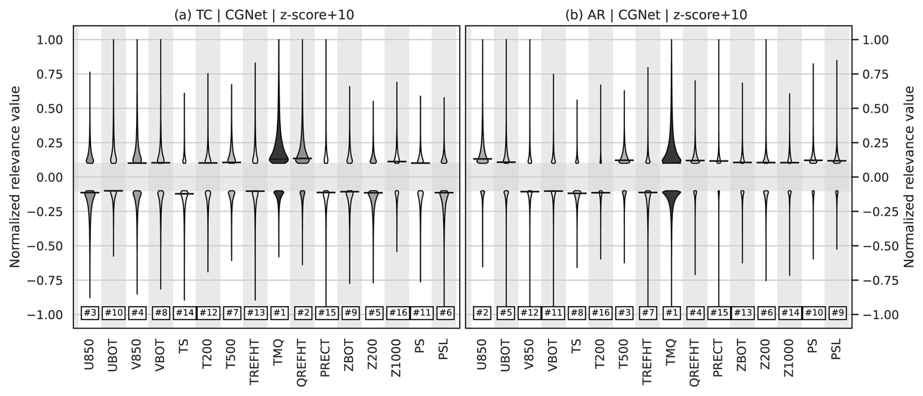
Figure 10 Distributions of relevance values (computed from test dataset) for CGNet trained with all 16 variables contained in the ClimateNet dataset, for (a) TC and (b) AR features. Z-score normalization shifted by +10 is used on all inputs for the reasons discussed in Sect. 6. Width of violin plots is differently scaled for TCs and ARs but consistent for all variables within (a) and (b). Relevance values in the range [−0.1…0.1] are omitted. Numbers at the bottom as well as grey shade indicate ranking in terms of numbers of grid points with absolute relevance > 0.1.

The analysis in Sect. 6 showed that for the different input variables, different fractions of grid points were found to be relevant in the different relevance intervals (numbers listed in Fig. 7). If a CNN is hence trained with all available input variables, distributions of relevance values can be computed for each input variable and the most relevant variables can be selected. We apply the approach to CGNet trained with z-score-normalized inputs shifted by +10 (cf. Sect. 6), to avoid the “ignorance-to-zero-input issue” (M22). Figure 10 shows violin plots (Hintze and Nelson, 1998) of the relevance distributions for each of the 16 ClimateNet variables. As in Sect. 6, we omit absolute relevance below 0.1. Variables are shown on the same order as in Table 1; the given ranking is based on the number of grid points with absolute relevance larger than 0.1.

Indeed, TMQ is found to be the most relevant input variable for both TC and AR detection. For TCs, the QREFHT variable is also considered relevant by CGNet. However, it should be closely correlated with TMQ. U850 and V850 are third and fourth, followed by several other variables of similar relevance. Some variables including TS, PS, and Z1000 are hardly of relevance. For ARs, U850 is also considered relevant; however, V850 is not. The results suggest, however, that AR detection could benefit from including T500 in the set of input variables. These findings, of course, can be expected due to existing meteorological knowledge (Gimeno et al., 2014). It is promising, however, that LRP analysis again provides plausible results.

Table 3 shows IoU scores for CGNet trained with all 16 input variables, the KS20 subset of TMQ, PSL, V850, and U850, as well as different selections that could be inferred from Fig. 10. The scores are largely of the same order; notably the three-input subset of TMQ, V850, U850 used by M22 achieves even higher scores than the KS20 subset and the 16-variable setup. Only when even more inputs are withdrawn does the detection performance drop, although it remains remarkably high. We note, however, that for every setup a relevance analysis as in Sects. 5 and 6 should be carried out to ensure plausible results.

We also note that since the size of the ClimateNet dataset is limited (cf. Sects. 2 and 3), we split the data into training and test parts only (cf. Sect. 2). Relevant variables were determined based on the test data (Fig. 10). The retrained CGNet setups in Table 3 were again evaluated on the test data. Some care needs to be taken with the results of this approach, as the variables found to be relevant could potentially be relevant mostly for the test data. If a larger dataset were available, an improved setup would split the data into three parts, also including a validation part (e.g., Bishop, 1995) for evaluating the results of the retrained setups.

Table 3 IoU scores reached by CGNet trained for different input variable combinations, using z-score normalization shifted by +10 for all input variables. All values are in percentages. The highest score per column is written in bold. Compare to Table 2.

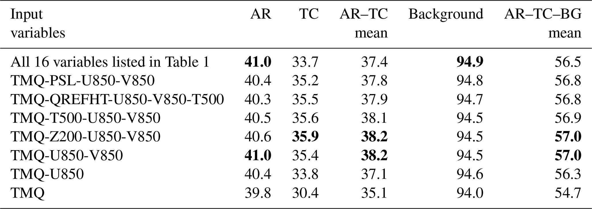
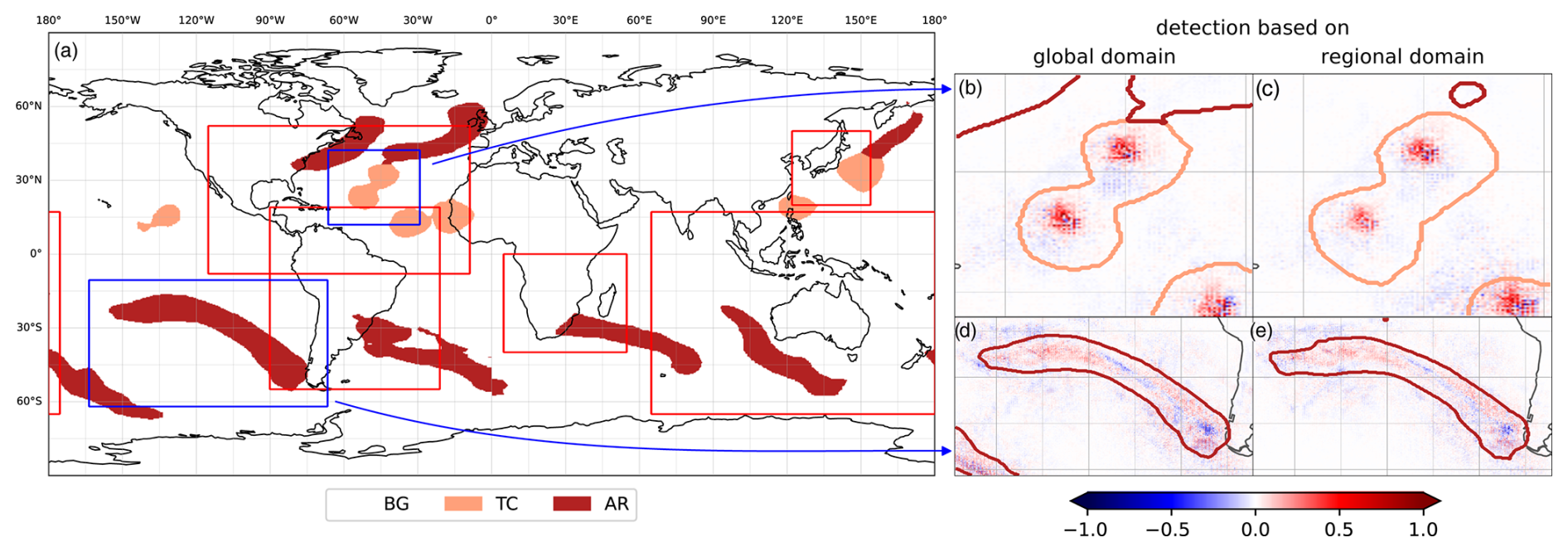
Figure 11 Regional domains to evaluate the robustness of feature detection when the CGNet trained on global data is applied with data on a regional domain. Same case and CGNet setup (KS20 setup and z-score normalization) as in Figs. 3 and 6. Blue bounding boxes in (a) surround selected TC and AR features; spatial relevance patterns in these regions is shown (b, d) for global data input into CGNet, and then the subregion is cut out from the global result, and (c, e) for only subregion data input into CGNet. Note that here relevance values are summed over all variables. Red bounding boxes in (a) show domains of regional NWP models: HAFS-SAR (North Atlantic), Eta (South America), SADC region (southern Africa), MSM (Japan), and ACCESS-R (Oceania). Domains are approximate where model domains are not rectangular in longitude and latitude.

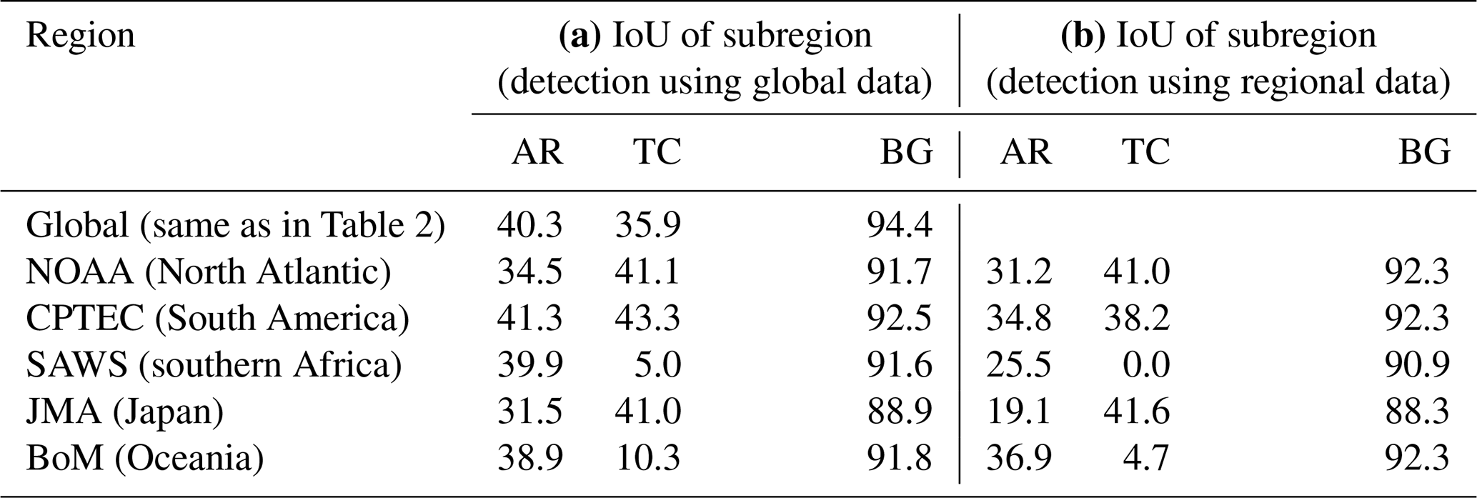
Table 4 IoU scores for TC and AR detection in subregions used by different regional NWP models. CGNet with the KS20 setup and z-score normalization is used (as for Figs. 3 and 6). Scores are computed (a) for global data input into CGNet, and then the subregion is cut out from the global result, and (b) for only subregion data input into CGNet.

Regarding A2, consider that in both operational weather forecasting and atmospheric research, numerical weather prediction (NWP) models with a regional domain are frequently used. The analysis discussed in the previous sections was based on global data. Could the CGNet trained on global data be also used with data from a regional domain, or would it have to be retrained? The analysis of spatial relevance patterns in Sect. 5 suggested that CGNet mostly considers grid points within or in close vicinity of a detected feature; hence we see a chance that detection with regional data could work “out of the box”. This would be valuable for cases where CNN training is expensive (e.g., Niebler et al., 2022, reported high computational demand for training their front-detection CNN), as a CNN trained globally could be applied to different regional models.

We consider our case from Sect. 5 and compare detected features and spatial relevance patterns (1) if the detection is based on global data as in the previous sections, and then the subregion is cut out, and (2) if the detection is based on regional data input into CGNet trained on global data. For our experiments, we simply cut out data from the global ClimateNet data; i.e., the grid point spacing is unchanged. Figure 11 shows how the detection result changes for two selected TC and AR features (blue boxes in Fig. 11a). Figure 11b and d show the features and relevance patterns when global data are used and Fig. 11c and e when regional data are used for testing. Note that for simplicity of display, the relevance of all four input variables is averaged in Fig. 11. Also note that for the regional domains, circular padding (cf. Sect. 3) is not suitable; here replicate padding is used instead.

Figure 11b–e show that the features at the center of the regional domains are fully detected with high similarity between both approaches. In contrast, the features only partially included in the region are not or not completely detected. These findings are plausible given that due to the convolutional architecture of CGNet, some area around a feature is required for detection. It is noticeable, however, that the inclusion of the TC center in the southeastern corner of Fig. 11b and c seems to be sufficient to detect the partially included TC. This is also further evidence for our hypothesis from Sect. 5 that the distance to a TC center plays a crucial role in the detection process. Also note that from the AR in the northeastern part of Fig. 11b, a small part is still detected in the regional data (Fig. 11c). Unlike rule-based systems that often define a minimum size for an AR feature (Shields et al., 2018), CGNet seems to not learn such size limitations.

The selected case provides promising evidence that indeed the CGNet trained on global data could be used for detecting features in regional data as well. For a more complete picture, we consider several regional domains used by national weather services (red boxes in Fig. 11a): the National Oceanographic and Atmospheric Administration (NOAA) in the USA (Dong et al., 2020), the Center for Weather Forecasting and Climate Studies (CPTEC) in Brazil (Alves et al., 2016), the South African Weather Service (SAWS; Mulovhedzi et al., 2021), the Japan Meteorological Agency (JMA; Saito et al., 2006), and the Australian Government Bureau of Meteorology (BoM; Puri et al., 2013). Table 4 lists IoU scores for the respective regional domains, again for feature detection based on (1) global data and (2) regional data. Despite using the same input data for detection, the IoU scores for (1) differ from the global IoU scores listed in Table 2 since only subsets of all features are present in the regional domains. Scores roughly deviate more from Table 2 for smaller subregions. For (2), IoU scores are lower compared to (1) for all subregions. This, however, is plausible considering the above discussion that features included only partially in a subregion are less well detected when only regional data are input to CGNet. The differences in IoU scores that we observe between approaches (1) and (2) are smaller for TCs (maximum difference of 5.6 % in Oceania) and more substantial for ARs (difference of up to 14.4 % for the southern African region and 12.4 % for the Japanese region). Our hypothesis is that this is due to the smaller size of TCs, which are hence more often completely contained in a subregion. Similarly, larger regional grids show higher IoU scores, possibly for the same reason of containing more complete features.

Concluding, we note that while detection performance decreases when regional data are used for testing, we argue that the method still has value, e.g., to assist forecasters in becoming aware of potentially important features. Also, the issue of decreased detection performance for only partially contained features in a region also affects rule-based detection methods, e.g., if rules with respect to feature size are used.

Results for A1 and A2 when using U-Net instead of CGNet are provided in the Supplement (Figs. S10 and S11; Tables S1 and S2 in the Supplement). Both CNN architectures again yield very similar results. Notably, regarding A1, the U-Net setup also considers TMQ to be the most relevant input; however, in contrast to CGNet the TS input provides more information.

8 Summary and conclusion

We adapted the xAI method Layer-wise Relevance Propagation, widely used in the literature for classification tasks, to be used for semantic segmentation tasks with gridded geoscientific data. We implemented the method for use with the CGNet and U-Net CNN architectures (Fig. 1) and investigated relevance patterns these CNNs learned for detection of 2-D tropical cyclone and atmospheric river features. Our analysis built on previous work by KS20, P21, and M22. In this paper, we focused on the CGNet setup suggested by KS20 using the four gridded and z-score-normalized input variables TMQ, PSL, U850, and V850 from the ClimateNet dataset provided by P21 (Table 1). Comparative results for U-Net are provided in the Supplement. The main findings from our study are as follows:

• With both CGNet and U-Net we were able to reproduce KS20 and P21 results with similar IoU scores (Sect. 3; Table 2).

• Adapting LRP (Fig. 2) to the semantic segmentation task provided the challenge of how to generalize the classification approach used by previous studies. We argue that averaging relevance from all grid points assigned to a feature provides meaningful results. Also, to use our method with the CGNet architecture, several layer-specific LRP calculation specifications had to be implemented for CNN layers specific to CGNet (Sect. 4).

• For the selected case, we found that CGNet learned physically plausible patterns for the detection task (Sect. 5). For TCs, relevant patterns include point-shaped extrema in TMQ and circular wind motion. For ARs, relevant patterns include elongated bands of high TMQ with different orientation on the Northern and Southern Hemisphere and eastward winds (Figs. 3 and 6).

• Spatial relevance is mostly locally confined around features, but analysis of the relevance of individual grid points indicated that for each grid point, CGNet uses its convolutional filters to account for the surrounding region (Fig. 4).

• CGNet makes use of both input values and the shape of patterns in the input fields. Analysis of input variable values at grid points that were attributed high relevance showed that, e.g., high values of TMQ are relevant for both TC and AR detection, however, that these high values are used for both pro and contra arguments for assigning a grid point to a feature (Sect. 6; Fig. 7). This behavior can be explained by the hypothesis that CGNet uses additional shape information for its decision. LRP does not provide information about shape relevance; however, composite maps we computed from all detected features provide strong evidence that TCs are detected as point-like structures and ARs as elongated bands (Fig. 7).

• Care needs to be taken when using LRP_z with z-score normalization (mapping the mean of a variable to zero and its standard deviation to ±1; as used by KS20, P21, and M22). CNNs including CGNet and U-Net include bias neurons to account for input data close to zero; however, LRP cannot attribute relevance to bias neurons. Hence, input values close to zero are assigned a relevance close to zero (referred to as the “ignorant-to-zero-input issue” by M22; cf. Fig. 6), even if the CNN does use the information via the bias neurons. As a workaround, we shifted the z-score-normalized data by +10 to avoid zero values (and also evaluated use of min–max normalization that maps variable values to 0…1). With these alternative normalizations, zero relevance around variable means disappears (Fig. 7), and spatial relevance patterns further suggest the role of shape information in the detection process (Fig. 8).

• LRP can be used for additional applications (Sect. 7). We demonstrated its use for finding the most relevant input variables to build a CNN setup by training CGNet with all 16 input variables in the ClimateNet dataset and then using relevance distributions to find the most relevant variables that need to be retained for a useful setup (Fig. 10 and Table 3). Also, we evaluated the robustness of detection when only data from subregions are used with the CGNet trained on global data. This has potential benefit to use a globally trained CNN for detecting features in data from regional NWP models. We find that due to the locality of relevance, features fully included in a subregion are well detected, while only partially contained features are not (Fig. 11 and Table 4).

Concluding, LRP in our opinion is a very useful tool to gain confidence for CNN-based detection of atmospheric features. For the case of TC and AR detection proposed by KS20 and P21, we find that their setup indeed learns physically plausible patterns for feature detection. We provide the source code of our implementation along with this paper and invite the geoscientific community to apply the method to further detection tasks. However, the open challenges of accounting for the relevance of bias neurons (“ignorant-to-zero-input issue”; M22) as well as for shape information need to be approached to be able to explain the behavior of CNNs for semantic segmentation tasks more completely. First work for accounting for bias relevance has recently been published in the computer vision literature (Wang et al., 2019), as has a method for accounting for shape information (Achtibat et al., 2023). These need to be adapted and potentially refined for geoscientific data. We look forward to future work in this direction.