AgriCarbon-EO v1.0.1: large-scale and high-resolution simulation of carbon fluxes by assimilation of Sentinel-2 and Landsat-8 reflectances using a Bayesian approach

Soil organic carbon storage is a well-identified climate change mitigation solution. Quantification of the soil carbon storage in cropland for agricultural policy and offset carbon markets using in situ sampling would be excessively costly, especially at the intrafield scale. For this reason, comprehensive monitoring, reporting, and verification (MRV) of soil carbon and its explanatory variables at a large scale need to rely on hybrid approaches that combine remote sensing and modelling tools to provide the carbon budget components with their associated uncertainties at intrafield scale. Here, we present AgriCarbon-EO v1.0.1: an end-to-end processing chain that enables the estimation of carbon budget components for major and cover crops at intrafield resolution (10 m) and regional extents (e.g. 10 000 km²) by assimilating remote sensing data (e.g. Sentinel-2 and Landsat8) in a physically based radiative transfer (PROSAIL) and agronomic models (SAFYE-CO2). The data assimilation in AgriCarbon-EO is based on a novel Bayesian approach that combines normalized importance sampling and look-up table generation. This approach propagates the uncertainties across the processing chain from the reflectances to the output variables. After a presentation of the chain, we demonstrate the accuracy of the estimates of AgriCarbon-EO through an application over winter wheat in the southwest of France during the cropping seasons from 2017 to 2019. We validate the outputs with flux tower data for net ecosystem exchange, biomass destructive samples, and combined harvester yield maps. Our results show that the scalability and uncertainty estimates proposed by the approach do not hinder the accuracy of the estimates (net ecosystem exchange, NEE: RMSE =1.68–2.38 gC m⁻², R²=0.87–0.77; biomass: RMSE =11.34 g m⁻², R²=0.94). We also show the added value of intrafield simulations for the carbon components through scenario testing of pixel and field simulations (biomass: bias $=-\mathrm{47}$ g m⁻², −39 % variability). Our overall analysis shows satisfying accuracy, but it also points out the need to represent more soil processes and include synthetic aperture radar data that would enable a larger coverage of AgriCarbon-EO. The paper's findings confirm the suitability of the choices made in building AgriCarbon-EO as a hybrid solution for an MRV scheme to diagnose agro-ecosystem carbon fluxes.

1 Introduction

Agriculture and land use changes account for 15 % (i.e. 8.7 Gt CO₂ yr⁻¹) of human-induced greenhouse gas (GHG) emissions (Pörtner et al., 2022; Skea et al., 2022). Agriculture has also been identified as a sector that can contribute to climate mitigation through several solutions (Porter et al., 2017; Matthews et al., 2022). Among these, soil organic carbon (SOC) storage has the potential to remove 0.6 to 9.3 Gt CO₂ yr⁻¹ globally from the atmosphere through the implementation of carbon farming practices (Skea et al., 2022). Increasing the SOC implies an enhancement of the net ecosystem carbon budget (NECB) (Woodwell and Whittaker, 1968; Chapin et al., 2006; Smith et al., 2010) expressed in Eq. (1). A positive variation of NECB can be achieved by increasing the gross primary production (GPP) and the net ecosystem exchange (NEE) through above-ground crop residue retention (Soussana et al., 2019; Bolinder et al., 2020), the addition of cover crops in crop rotations (Poeplau and Don, 2015; Lugato et al., 2020), and an increase in the carbon imports through the application of organic amendments (Bolinder et al., 2020) and biochar (Steinbeiss et al., 2009).

$$\begin{array}{}\text{(1)}& \textcolor{red}{}\end{array}$$

Equation (1) also shows the linkage between (1) the quantification of the effect of ecosystem respiration (R_eco), which is subdivided into autotrophic (plant) and heterotrophic (soil) respiration (R_auto and Rh), and (2) the quantification of carbon exports that correspond mainly to yield and the fraction of biomass incorporated to the soil. All the components in the equation are impacted not only by the intrinsic characteristics of the field (soil) and the weather but also, and most importantly, by the farming practices: choice of crop and cover crop, choice of amendments, and choice of harvesting, etc. The quantification of the carbon fluxes due to each of the components is the basis of the computation of the net ecosystem carbon budget, as shown in Eq. (1).

It should be noted that after the death of the vegetation, all the unharvested biomass returns to the soil. At this point, we can approximate that NECB=ΔSOC. The accumulation of SOC in agricultural soils, in addition to climate change mitigation, has additional benefits in terms of ecosystem soil services (ESSs), such as increasing soil fertility (Su et al., 2006), enhancing water-holding capacity (Karhu et al., 2011), and increasing biodiversity (Wall et al., 2015). SOC storage could also provide an additional source of revenue for farmers through carbon credits and subsidies.

Following the Intergovernmental Panel on Climate Change guidelines for national GHG inventories, methodologies for assessing SOC stock changes have been developed. They are based on a tiered approach with increasing complexity involving soil monitoring networks where SOC is directly measured and process-based modelling where ΔSOC is modelled by taking into account the soil, climate, and mean biomass returned to the soil (GPP–R_auto–C_export) derived from yield at the regional scale (Del Grosso et al., 2005; Yokozawa et al., 2010; Lehtonen et al., 2016). The need to monitor soil carbon at the farm and field levels to inform individual farmers and guide policies and the development of carbon markets has led to the development of monitoring, reporting, and verification (MRV) schemes based on similar approaches employed at a higher resolution (Smith et al., 2020; Paustian et al., 2019). These approaches are mainly used in carbon farming projects following national or regional initiatives (e.g. Label Bas Carbone in France). They often rely on a soil-centred quantification approach where the focus is the modelling of Rh, C imports, and C exports. In these approaches, the estimates of carbon returned to the soil are usually extrapolated from farm- or field-scale yield information (Clivot et al., 2019). The field scale often does not match the intrafield/farm variability of the soil characteristics and plant growth (de Gruijter et al., 2016; Ellili et al., 2019). This means that these values present limitations in terms of accuracy and spatial representativity.

Coupled plant–soil process-based models that address the quality and quantity of the crop residues that return to the soil are also used to assess SOC stock changes. These models include the main components of the cropland's biological CO₂ fluxes. They can also account for carbon inputs through organic fertilization and carbon exports of biomass at harvest (Eq. 1, Smith et al., 2010). Existing agronomic models, such as DSSAT-CSM (Porter et al., 2010), STICS (Launay et al., 2021), DAYCENT (Parton et al., 1998), and WOFOST (Supit et al., 1994); soil models, for example, DNDC (Gilhespy et al., 2014); and land surface models, for example, ORCHIDEE-STICS (Gervois et al., 2008), take into account a wide array of environmental conditions to represent crop growth and the components of the carbon budget (Eq. 1). However, water and nutrient availability, local topography, pests, and historical factors (e.g. former ditches, roads, field limits) highly influence soil and plant processes (Gregory et al., 2009). This can result in high spatiotemporal variability in crop development and soil processes that can be observed, even at the intrafield scale (Stevens et al., 2008; de Gruijter et al., 2016). Moreover, to operate those models, farmer activity data and crop development dynamics are required to provide accurate estimates of SOC stock changes. Getting hold of this information at a large scale is still challenging (Seidel et al., 2018; Wattenbach et al., 2010). However, it is possible to use time series of biophysical variables such as green leaf area index (GLAI), derived from remote sensing data, to provide information about development dynamics to those models through data assimilation (Huang et al., 2019; Battude et al., 2017; Pique et al., 2020a). These assimilated observations provide spatially explicit crop-specific estimates of biomass and carbon returned to the soil using coupled soil–plant models. Assimilation of biophysical variables is usually based on iterative optimization methods such as Simplex, Monte Carlo Markov chain (MCMC), ensemble Kalman filter, or variational assimilation that are generally applied at moderate resolutions (Kumar et al., 2019; Hararuk et al., 2014) or field scale (Trepos et al., 2020; Upreti et al., 2020). Applying these methods at an intrafield resolution over large areas is often computationally prohibitive. Enhancing scalability is thus key to assessing the spatial variability of CO₂ flux components at a scale consistent with measurements of soil and plant characteristics. Operating on a scale that is representative of measurements enables better diagnosis and calibration of plant and soil processes, as well as a more robust validation and uncertainty estimation of the model outputs.

This paper aims to present the newly developed AgriCarbon-EO processing chain for the assimilation of Earth Observation (EO) data into the SAFYE-CO2 agronomic model at a large scale (100 km) and intrafield resolution (10 m). This processing chain allows for the assessment of the carbon budget components (Eq. 1). The challenge of estimating the carbon budget components at high spatial resolution at a large scale is addressed by using the new BASALT (BAyesian normalized importance SAmpling via Look-up Table generation) algorithm, which also provides uncertainty estimates. In addition, the paper aims to provide an evaluation of the accuracy, limitations, and robustness of AgriCarbon-EO methods through validation exercises and scenario simulations. We chose to make these assessments for wheat in southwest France, as this area benefits from a large amount of data that has been gathered in the context of the Observatoire Spatial Regional (OSR) and the Integrated Carbon Observation System (ICOS) network. Furthermore, southwest France is a major production area of wheat. This area has also been chosen because it presents a challenge for spatial crop modelling in reproducing the diverse crop growth dynamics induced by a wide array of pedo-climatic conditions in a hilly landscape. The scenario simulations were designed to assess the robustness of the method with respect to the amount of assimilated remote sensing data and the added value in using high-resolution agronomic modelling.

In the following sections, we first present the details of the AgriCarbon-EO processing chain including the standard inputs, models, and BASALT assimilation scheme. We then present the numerical experimental setup and the validation datasets. Next, we present the validation results and the impact of image availability. Finally, we conclude with the benefits and limitations of the presented solution for assessing the cropland carbon budget components and their associated uncertainties at high resolution over large areas.

2 AgriCarbon-EO chain

2.1 Overview of the processing chain

AgriCarbon-EO is an end-to-end processing chain that simulates multiple relevant variables of crop development, biomass inputs to the soil, CO₂ fluxes, and water fluxes at a daily timescale, for the assessment of carbon and water budgets. It is specifically designed to assimilate optical remote sensing datasets at native high resolution into a parsimonious agronomic model (SAFYE-CO2) over large regions. A brief description of the data flow and processing steps is presented here (Fig. 1) and detailed in the following subsections:

1. A preprocessing “data ingestion” step allows the updating of existing datasets through the automated downloading and stacking of satellite images and weather forcing. Optical bottom-of-atmosphere (BOA) reflectances are downloaded for Sentinel-2 and Landsat-8 (referred to as S2 and L8 below). The weather data are stored in time series with the associated correspondence matrix to the high-resolution grid defined by the user. This is performed for the zone defined by the input land cover (polygons or mask raster map).

2. The biophysical variable GLAI is retrieved from the satellite reflectance images by inverting a radiative transfer model (PROSAIL). The retrieval of GLAI is based on an adapted Bayesian importance sampling procedure (i.e. BASALT).

3. The crop model (SAFYE-CO2) parameters are inverted by assimilating the GLAI time series using the BASALT method as in the previous step. In this case, LUTs are generated based on the closest known weather simulation node. Only the phenological crop model parameters and the light use efficiency (LUE) are inverted in this procedure.

4. A postprocessing step allows the construction of the output products based on the posterior crop model parameter distribution. Georeferenced maps of the variables of interest in each model (i.e. PROSAIL, SAFYE-CO2) are constructed as well as cumulative variables (e.g. NEP, which is the cumulative NEE over 1 cropping year, number of satellite acquisitions, and soil water content).

AgriCarbon-EO is implemented in the Python language. A maximum requirement of 5 GB per process for the satellite images needs to be considered. This will allow mono-process tests and development on standard computers over smaller study areas, as well as large-scale applications (e.g. 100×100 km) with high-performance-computing (HPC) resources.

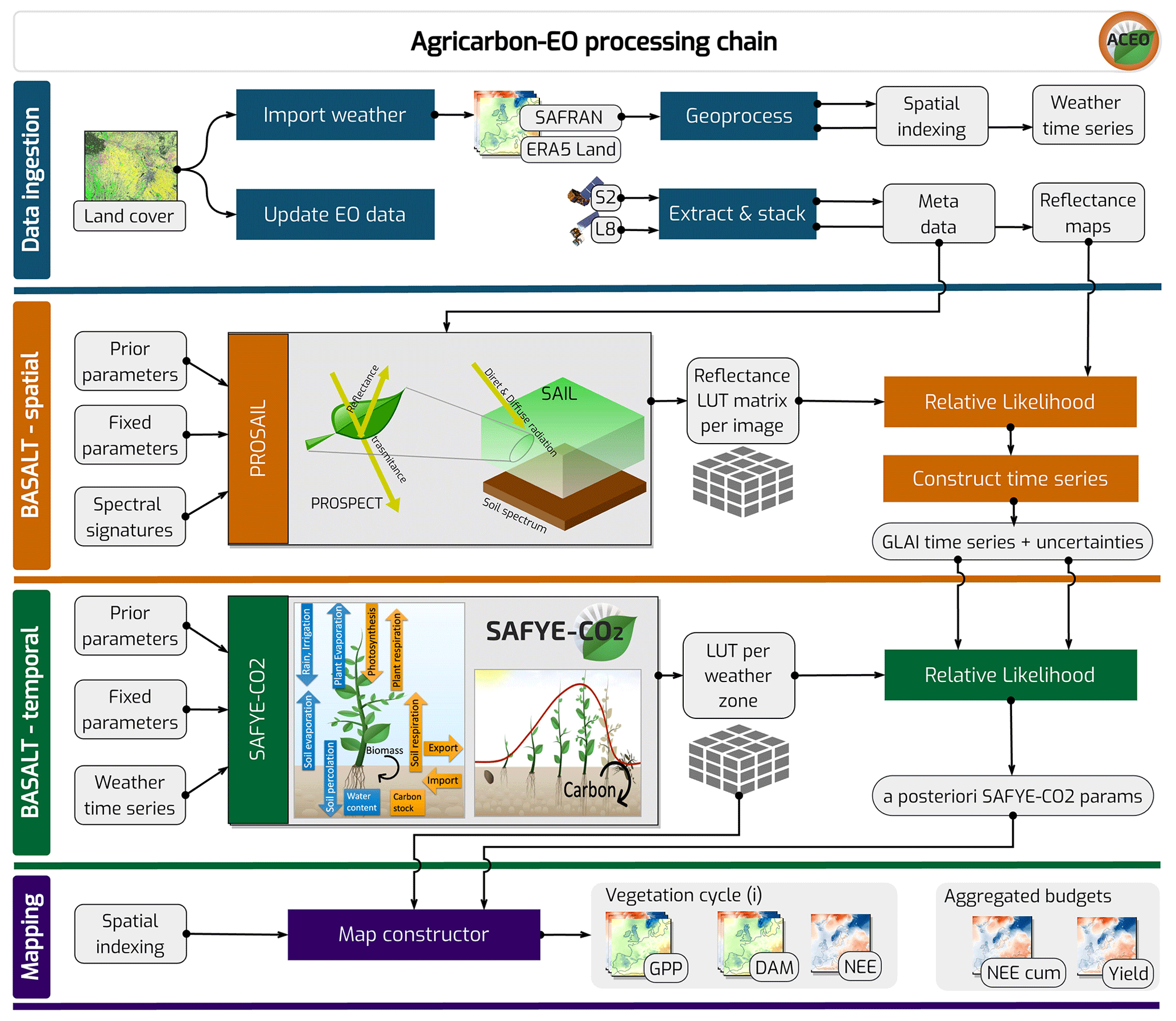
Figure 1 Overview of the AgriCarbon-EO data flow and main processing steps that include the data ingestion, BASALT spatial retrieval, BASALT temporal retrieval, and mapping of the variables of interest.

2.2 Input dataset

In the following subsections, the spatial datasets needed for AgriCarbon-EO are detailed.

2.2.1 Land cover map

The main driver for the data preparation is a land cover (LC) map in vector or raster format. This file contains the boundaries of each agricultural field for a given cropping year over a selected region of interest or a raster-based mask. Based on the border extents of the LC map, the remote sensing and weather forcing data are downloaded and preprocessed. When the simulations are intended to cover several cash crop cycles, a run scenario of AgriCarbon-EO is considered for each individual crop cycle. Additionally, a standard simulation can include a cover crop with each cash crop. In this paper, AgriCarbon-EO was applied to winter wheat crops in southwest France (on the Sentinel-2 tile referenced as 31TCJ) in 2017, 2018, and 2019. The LC map was obtained from the Registre Parcellaire Graphique (RPG) in France (RPG, 2021), which is available online in Open Licence v2.0. This information is produced by the Institut Geographique National (IGN) for the Agence de Service de Paiement (ASP; i.e. the French Agency for Services and Payment) in charge of the implementation, control, and payment of the subsidies for the EU Common Agricultural Policy (CAP) in France. In this study, the original polygons in the Lambert-93 projection (EPSG:2154 – RGF93) were reprojected to a selected common grid projection: WGS 84/UTM31.

2.2.2 BOA surface reflectances

The assimilated remote sensing data are optical multi-spectral surface reflectances at the BOA, which correspond to reflected energy from the top of the canopy and the soil at a given incidence angle. Currently, AgriCarbon-EO uses data from the ESA's Sentinel-2 programme (Drusch et al., 2012) and NASA's Landsat-8 programme (Roy et al., 2014), knowing that the modular interface is compatible with multisource EO data. The Sentinel-2 data are acquired over 13 optical bands with a resolution of 10 to 60 m depending on the spectral bands with a 5 d revisit from the constellation. Only the nine visible bands were considered from the Landsat-8 data. Landsat-8 has a revisit of 16 d and a spatial resolution of 30 m in the visible range.

For this study, the data were downloaded from the Thematic Center for Continental Surfaces (THEIA), which uses a common atmospheric correction and cloud masking algorithm for Sentinel-2 and Landsat-8 through the MAJA processing chain (Hagolle et al., 2021). This enables a harmonized Level-2A database with an efficient cloud masking algorithm (Baetens et al., 2019). The data contain quality indicators, including cloud coverage. The dataset is presented as granules (tiles) of 110×110 km orthoimages in the UTM projection. Prior to the processing, the remote sensing datasets are decompressed and resampled at 10 m resolution using the nearest-neighbour method.

2.2.3 Weather forcing data

Daily weather data maps covering the simulation period and spatial extents are used to force the crop model. Cumulative daily global incoming solar radiation (R_g in MJ m⁻²) and daily average air temperature at 2 m (T_a in ^∘C) are needed for the vegetation growth module in SAFYE-CO2. Based on previous studies that showed the impact of diffuse radiation on crop development and photosynthesis (Béziat, 2009; Roderick et al., 2001), the diffuse incoming radiation is computed based on De Jong (1980). Two additional forcings are needed for the water budget module of SAFYE-CO2: daily potential evapotranspiration (ET0 in mm d⁻¹) and daily cumulative rainfall (rain in mm d⁻¹). AgriCarbon-EO supports two data sources that provide weather data: the Météo-France SAFRAN dataset (Vidal et al., 2010) and ERA5 Land (Muñoz-Sabater et al., 2021). The extraction of the ERA5 Land data was performed via the dedicated API. SAFRAN consists of a reanalysis of climate variables at 8 km spatial resolution and an hourly timescale over France starting in 1958. In this paper, the weather data were extracted from the Météo-France SAFRAN dataset and reprojected over the UTM/31N at 8 km resolution.

2.3 Process-based models

2.3.1 Radiative transfer modelling using PROSAIL

Maps of geophysical variables (i.e. GLAI) are retrieved in AgriCarbon-EO by inverting the PROSAIL radiative transfer model. PROSAIL has been extensively used as a radiative transfer model for vegetated areas (Jacquemoud et al., 2009) with a wide range of inversion schemes (Wang et al., 2022). PROSAIL combines the PROSPECT and SAIL models (Baret et al., 1992). PROSPECT provides leaf spectral properties in the 400 to 2500 nm wavelength (Jacquemoud and Baret, 1990). SAIL (scattering by arbitrary inclined leaves) is a multidirectional canopy reflectance model (Verhoef, 1984) based on the bidirectional reflectance model (Suits, 1971). A Python implementation of PROSAIL was used in AgriCarbon-EO. This version includes the coupled PROSAIL from PROSPECT-5-D (Féret et al., 2017), 4SAIL (Verhoef et al., 2007), and a simple Lambertian soil reflectance model. The PROSAIL parameters were inverted using a Bayesian approach to provide GLAI and its corresponding uncertainty as input to the crop model inversion.

2.3.2 Crop CO₂ fluxes and biomass modelling using SAFYE-CO2

SAFYE-CO2 is a parsimonious agronomic model that runs at a daily time step (Veloso, 2014; Pique et al., 2020a, b). The model stems from the SAFY models (Duchemin et al., 2008; Battude et al., 2017) which compute dry above-ground biomass (DAM), based on the LUE theory of Monteith et al. (1977). A full description of the SAFYE-CO2 model is provided in Veloso (2014); Pique et al. (2020a, b). The core equations of the model are detailed below. In SAFYE-CO2, NEE is computed based on Rh and net primary production (NPP; gC m⁻²), which in turn is computed from GPP (gC m⁻²) by subtracting autotrophic respiration R_auto (gC m⁻²), as presented in Eq. (1). The CO₂ fluxes caused by the plant, GPP, and R_auto are computed using Eqs. (2) and (10), respectively.

$$\begin{array}{}\text{(2)}& \mathrm{GPP}=R_{\mathrm{g}}\cdot {\mathit{ϵ}}_c{f}_T\left(T_{\mathrm{a}}\right)\cdot f_{\mathrm{w}}\left(\mathrm{WC}\right)\cdot \mathrm{ELUE}\cdot \mathrm{APAR}\cdot {\mathrm{SR}}_{\mathrm{10}},\end{array}$$

where R_g is the incoming global radiation (MJ m⁻² d⁻¹), f_T(T_a) is the temperature stress function that depends on T_a the mean air temperature at 2 m (^∘C), and f_w(WC) is the water stress function where WC is the soil water content (m⁻³ m⁻³). In this study, the water budget is computed, but the water stress function is deactivated (i.e. f_w(WC)=1). In Eq. (2), ELUE (gC MJ⁻¹ m⁻²) is the effective light use efficiency (Eq. 3).

$$\begin{array}{}\text{(3)}& \mathrm{ELUE}={\mathrm{LUE}}_a\times e^{(\frac{R_{\mathrm{diff}}}{R_{\mathrm{g}}}\cdot {\mathrm{LUE}}_b)},\end{array}$$

where LUE_a (gC MJ⁻¹ m⁻²) is the light use efficiency for direct radiation, and LUE_b is a correction coefficient for the impact of diffuse radiation R_diff (MJ m⁻² d⁻¹) on ELUE.

In Eq. (2), SR₁₀ accounts for the decrease in photosynthetic efficiency during senescence linked among others to the decrease in chlorophyll.

$$\begin{array}{}\text{(4)}& \begin{array}{rl}{\mathrm{SR}}_{\mathrm{10}}={\displaystyle \frac{\mathrm{GLAI}}{\mathrm{GLAI}\mathit{\_}\max \times \mathrm{Cs}}}& \text{if}\mathrm{SMT}>{\mathrm{Sen}}_{\mathrm{a}}.\\ & \text{else}{\mathrm{SR}}_{\mathrm{10}}=\mathrm{1},\end{array}\end{array}$$

where Cs is the parameter that controls the slope of SR₁₀ depending on the thermal age of the crop SMT, and Sen_a refers to the thermal age at which the plant enters senescence. Finally, FAPAR is the fraction of absorbed photosynthetically active radiation and is computed in SAFYE-CO2 (Eq. 5).

$$\begin{array}{}\text{(5)}& \mathrm{FAPAR}={\mathit{ϵ}}_c\cdot \mathrm{1}-e^{\mathrm{Kex}\cdot \mathrm{GLAI}},\end{array}$$

where ϵ_c is the parameter that quantifies the fraction of photosynthetically active radiation in R_g.

SAFYE-CO2 derives GLAI (Eq. 6) and other phenotypic traits using allometric coefficients and the plant's organ biomass values such as DAM, dry leaf biomass (DLM), and dry below-ground biomass (DBM) (Eq. 7). To compute these biomass values, the model relies on partition coefficients that dispatch the carbon and resulting biomass in different organs depending on the thermal age of the crop (Eq. 8, Baret et al., 1992).

$$\begin{array}{}\text{(6)}& \left\{\begin{array}{l}\mathrm{\Delta }{\mathrm{GLAI}}^{+}=\mathrm{DLM}\cdot \mathrm{SLA}\\ \mathrm{\Delta }{\mathrm{GLAI}}^{-}=\mathrm{GLAI}\cdot (\mathrm{SMT}-{\mathrm{Sen}}_{\mathrm{a}})\cdot {\mathrm{Sen}}_b^{-\mathrm{1}},\end{array}\right.\end{array}$$

where SLA (m² g⁻¹) is the specific leaf area, and Sen_b is the rate of functional leaf loss depending on thermal age.

$$\begin{array}{}\text{(7)}& \left\{\begin{array}{l}\mathrm{\Delta }\mathrm{DAM}=\frac{\mathrm{NPP}}{{\mathrm{C}}_{\mathrm{veg}}}\cdot (\mathrm{1}-\mathrm{PRT}\mathrm{\_}\mathrm{R})\\ \mathrm{\Delta }\mathrm{DLM}=\mathrm{\Delta }\mathrm{DAM}\cdot \left(\mathrm{PRT}\mathrm{\_}\mathrm{L}\right)\\ \mathrm{\Delta }\mathrm{DBM}=\frac{\mathrm{NPP}}{{\mathrm{C}}_{\mathrm{veg}}}\cdot \left(\mathrm{PRT}\mathrm{\_}\mathrm{R}\right),\end{array}\right.\end{array}$$

where C_veg is the average fraction of carbon in plant biomass.

$$\begin{array}{}\text{(8)}& \left\{\begin{array}{ll}\mathrm{PRT}\mathrm{\_}\mathrm{R}& =\mathrm{PRT}\mathrm{\_}\mathrm{Rb}+(\mathrm{PRT}\mathrm{\_}\mathrm{Ra}-\mathrm{PRT}\mathrm{\_}\mathrm{Rb})\\ & \cdot e^{(-\mathrm{PRT}\mathrm{\_}\mathrm{Rc}\cdot \frac{\mathrm{SMT}}{\mathrm{SMT}\mathrm{\_}\mathrm{G}})}\\ & \text{if}\mathrm{PRT}\mathrm{\_}\mathrm{R}>\mathrm{0}\text{else}\mathrm{PRT}\mathrm{\_}\mathrm{R}=\mathrm{0}\\ \mathrm{PRT}\mathrm{\_}\mathrm{L}& =\mathrm{1}-\mathrm{PRT}\mathrm{\_}\mathrm{La}\cdot e^{\mathrm{PRT}\mathrm{\_}\mathrm{Lb}\cdot \mathrm{SMT}}\\ & \text{if}\mathrm{PRT}\mathrm{\_}\mathrm{L}>\mathrm{0}\text{else}\mathrm{PRT}\mathrm{\_}\mathrm{L}=\mathrm{0}\end{array}\right.\end{array}$$

The fraction of biomass allocated below ground, PRT_R, is computed using PRT_Ra, PRT_Rb, PRT_Rc, and SMT_G, which correspond to the end-of-cycle fraction of biomass allocated below ground, the initial fraction of biomass allocated below ground, a coefficient modulating the decrease in biomass partition to the roots between the initial and end-of-cycle states, and the sum of the temperature at which grain filling starts respectively. The fraction of above-ground biomass allocated to the leaves PRT_L is computed using PRT_La and PRT_Lb0, respectively, the initial fraction of the above-ground biomass that is not allocated to the leaves and a fitting parameter that modulates the rate and thus the end of allocation of above-ground biomass to the leaves.

The biomass and yield are used to determine carbon exports in Eq. (1). Equation (9) illustrates a simple way to estimate exported biomass by taking into account only the dry above-ground biomass (DAM), the harvest index (HI), and the fraction of carbon in the dry biomass (Cveg).

$$\begin{array}{}\text{(9)}& C_{\mathrm{exports}}=\stackrel{\text{dry yield}}{\overbrace{\mathrm{DAM}\times \mathrm{HI}}}\times {\mathrm{C}}_{\mathrm{veg}}\end{array}$$

The other component of NPP, R_auto, is divided into vegetation maintenance respiration R_maint (Amthor, 2000) and vegetation growth respiration Rgrow (Choudhury, 2000), as described in Eq. (10).

$$\begin{array}{}\text{(10)}& \left\{\begin{array}{l}{R}_{\mathrm{auto}}=R_{\mathrm{maint}}+R_{\mathrm{grow}},\text{where}\\ R_{\mathrm{maint}}=R_{\mathrm{10}}\cdot Q_{\mathrm{10}}^{-\mathrm{0.1}\cdot (T-\mathrm{10})}\cdot {\mathrm{SR}}_{\mathrm{10}}\text{and}\\ R_{\mathrm{grow}}=(\mathrm{1}-Yg)\cdot (\mathrm{GPP}-{\mathrm{R}}_{\mathrm{maint}})\end{array}\right.\end{array}$$

R_maint depends on two parameters: the basal plant respiration at 10 ^∘C (R₁₀), the temperature sensitivity of plant respiration (Q₁₀), and the temperature T and SR₁₀ to represent an increase in relative maintenance cost during senescence. The growth respiration is computed from the growth conversion efficiency, GPP, and R_maint.

The final term in NEE, Rh (gC m⁻²), is computed using the empirical model in Delogu et al. (2017) that depends on soil moisture and temperature.

$$\begin{array}{}\text{(11)}& \left\{\begin{array}{l}\mathrm{Rh}={\mathrm{Rh}}_{\mathrm{1}}\cdot e^{({\mathrm{Rh}}_{\mathrm{2}}\cdot T_{\mathrm{soil}})}\cdot H_{\text{water stress,}}\text{where}\\ H_{\text{water stress}}=(\mathrm{1}+{\mathrm{Rh}}_{\mathrm{1}}\cdot e^{({\mathrm{Rh}}_{\mathrm{2}}\cdot \mathrm{RSM}\mathrm{1})}{)}^{-\mathrm{1}}\end{array}\right.\end{array}$$

Rh₁ is the reference Rh rate, Rh₂ expresses the RH sensitivity to temperature, and H_water-stress is the effect of soil moisture on soil carbon decomposition. In H_water-stress, Rh_H1 and Rh_H2 provide the form of the water stress function and RSM1 the relative soil moisture.

A Python implementation of SAFYE-CO2 was developed for AgriCarbon-EO and is used in this paper. This new version is vectorized to provide predictions for multiple runs and build LUTs. It can also handle multiple vegetation cycles for each run (e.g. crop and cover crop) and has a modular architecture. The physical modules are restructured to regroup soil processes, plant phenology, plant physiology, heterotrophic activity, and field management.

In SAFYE-CO2, the water flux computation is based on the Penman–Monteith and FAO-56 methodologies that enable the computation of evapotranspiration and water distribution in the soil based on a bucket model (Allen et al., 1998). The coupling between the carbon and water cycles occurs in two ways. Plant growth impacts root water uptake, and the soil water content impacts GPP production through a water stress coefficient. The dynamic computation of GLAI in Eq. (6) provides the link between the model and the GLAI retrieved from optical EO and therefore allows us to constrain the model's phenological and light use efficiency parameters (emerg, PRT_La, PRT_Lb, SLA, Sen_a, Sen_b, Harv, LUEa) using EO data assimilation. The assimilation of GLAI allows implicit accounting of soil stress impacts (e.g. nutrients and water) on vegetation development. Therefore, the water stress effect on GPP and plant development is implicitly accounted for through the model's parameters, resulting mainly in lower values of LUE for a field experiencing water stress. Assimilating GLAI also enhances the estimation of NEE and the export of specific organs and the resulting NECB (Eqs. 9 and 1) by considering the effect of the crop growth dynamic. In data assimilation, the relative parsimony of SAFYE-CO2 compared to models such as STICS (Dumont et al., 2014) or DSSAT (Porter et al., 2010) entails a limited number of free parameters controlling the vegetation dynamics. This allows the use of scalable assimilation algorithms such as “BASALT” presented below that can only be applied to relatively low dimensional optimization problems (Bellman, 2015).

2.4 Bayesian normalized importance SAmpling using Look out Table – BASALT

To provide large-scale high-resolution assimilation, a tailored inversion method was developed. The new approach, BASALT, relies on the Bayesian normalized importance sampling (NIS) approach to address the need for uncertainty propagation across the processing chain. Also, the generation of look-up tables (LUTs) provides computational gain by reducing the total number of model simulations. In a Bayesian framework, the initial knowledge about the model's parameters is represented by a probability distribution P(Θ), the prior distribution. The knowledge brought by the observations x is expressed by the conditional probability distribution P(Θ|x) of the model parameters knowing the observations x, the so-called posterior distribution. The goal is to evaluate this posterior distribution using Bayes' theorem that connects P(Θ|x), P(Θ), and P(x|Θ), called the likelihood (Eq. 12):

$$\begin{array}{}\text{(12)}& P\left(\mathrm{\Theta }\right|x)={\displaystyle \frac{P\left(x\right|\mathrm{\Theta }\left)P\right(\mathrm{\Theta })}{P\left(x\right)}}.\end{array}$$

P(x) is the probability of observation (marginal distribution). Bayesian methods are at the root of popular inversion algorithms such as MCMC or Dream (Vrugt, 2016). Such algorithms have often been applied to agronomic modelling (Dumont et al., 2014), ecosystem modelling (Ma et al., 2022), and radiative transfer modelling (Zhang et al., 2005).

In BASALT, random samples are generated for the model according to the probability distribution that best represents the user's prior knowledge of the model's parameters. The model output variables are calculated for each of those samples, given forcing and fixed parameters specific to a spatial and/or temporal range. The sampled parameters and resulting variables are treated as an LUT containing the prior state of the model for the range where the forcing is valid. Following LUT creation, the different LUT entries are compared against observations with known uncertainty. Using a normal error model for the observation allows log-likelihoods to be computed as presented in Eq. (13). Following this step, the relative likelihoods (RLs) of each LUT entry can be computed as presented in Eq. (14). In AgriCarbon-EO, this can be done for different scales, i.e. the entity scales or the scale of a group of entities. Finally, the posterior distribution is computed based on the underlying error model with a normal distribution by computing a weighted mean and standard deviation (Eq. 15).

$$\begin{array}{}\text{(13)}& \begin{array}{rl}\log L_{i,j}& =\sum \left(-{\displaystyle \frac{\mathrm{1}}{\mathrm{2}}}\log (\mathrm{2}\mathit{\pi }\left({\mathit{\sigma }}_{o,i,j}{)}^{\mathrm{2}}\right)\right)\\ & -{\displaystyle \frac{\left(v_{o,i,j}-{\mathit{\mu }}_{o,i,j}^{\mathrm{2}}\right)}{\mathrm{2}{\mathit{\sigma }}_{o,i,j}}},\end{array}\end{array}$$

where v is the simulation value, μ and σ are the mean and standard deviation of the observation, j is the index for entities, o is the index of the independent observations, and i is the index for the model run in the LUT.

$$\begin{array}{}\text{(14)}& {\mathrm{RL}}_i={\displaystyle \frac{e^{\log L_i}}{{\sum }_i{e}^{\log L_i}}};{\mathrm{RLfield}}_i={\displaystyle \frac{{\sum }_k{\mathrm{RL}}_{i,k}}{{\sum }_i{\sum }_k{\mathrm{RL}}_{i,k}}},\end{array}$$

where RL_i is the relative likelihood at the entity scale, k is the entities in the same field, and RLfield_i is the relative likelihood at the field scale assuming an equal contribution of each pixel in the field.

$$\begin{array}{}\text{(15)}& \begin{array}{rl}{\mathit{\mu }}_{\mathrm{w}}(v_i,{\mathrm{RL}}_i)& ={\displaystyle \frac{{\sum }_i{v}_i{\mathrm{RL}}_i}{{\sum }_i{\mathrm{RL}}_i}};\\ & {\mathit{\sigma }}_{\mathrm{w}}(v_i,{\mathrm{RL}}_i,{\mathit{\mu }}_{\mathrm{w}})={\displaystyle \frac{{\sum }_i(v_i-{\mathit{\mu }}_{\mathrm{w}}{)}^{\mathrm{2}}\cdot {\mathrm{RL}}_i}{{\sum }_i{\mathrm{RL}}_i}},\end{array}\end{array}$$

where μ_w is the weighted mean, v_x is the vector given by the LUT for a parameter or variable, x is the number of samples, and σ_w is the weighted standard deviation.

2.4.1 Retrieval of GLAI maps from PROSAIL

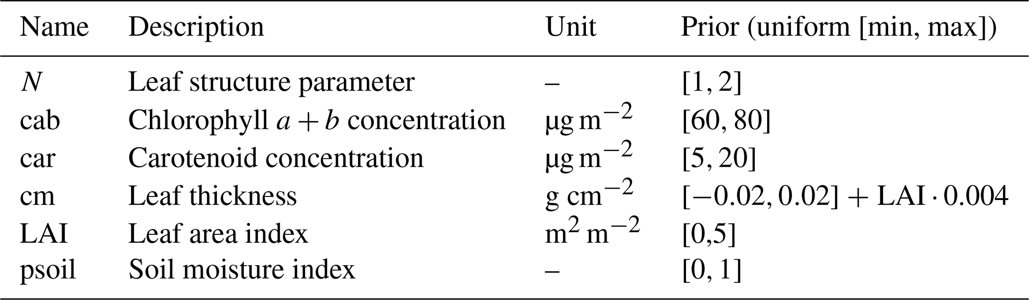
When inverting PROSAIL, the main objective is to retrieve GLAI and its associated uncertainties that will be assimilated by SAFYE-CO2. This is done by generating an LUT of PROSAIL runs (size =5000) for each remote sensing image based on the prior (Table 1) and the solar and observation angles provided by Sentinel-2 and Landsat-8 products. Equation (14) is then used to evaluate the RL, where j is the index of pixels in the simulated image, i is the index of the PROSAIL runs in the LUT, and o is the observed reflectances from the Sentinel-2 or Landsat-8 images. As PROSAIL provides LAI and not GLAI, the chlorophyll content (cab) is constrained to a high interval [60,80] µg m⁻². This makes all simulated surfaces green and thus allows GLAI to be retrieved. A constraint is also added to the relation between dry biomass and GLAI to reduce the parameter search space by eliminating solutions with leaves that are too thin or thick. Then, the surface reflectances of the Level 2-A BOA products are considered to follow a normal distribution with a mean and a standard deviation that is fixed at 0.02. Finally, the posterior distribution is approximated with a normal distribution, using Eq. (15), to determine μ and σ.

Table 1 Priors' configuration for PROSAIL parameters used in the Bayesian inversion.

2.4.2 Application of BASALT to SAFYE-CO2

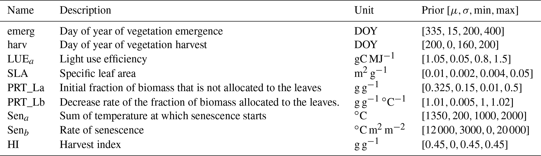
The simulated variables, DAM, yield, GPP, R_eco, and NEE, are highly dependent on the duration and intensity of crop development (Ceschia et al., 2010). The GLAI outputs from PROSAIL are assimilated into SAFYE-CO2 to correct the prior vegetation dynamics. This is done by generating a LUT of SAFYE-CO2 runs (size =5000) for each zone with the same forcing (i.e. same prior). In this case, the zoning is defined by the weather forcing data (i.e. SAFRAN at 8 km). For each zone, Eqs. (13) and (14) are applied to evaluate the RL given the GLAI observations, where j is the index of pixels in the simulated area, i is the index of the SAFYE-CO2 runs in the LUT, and o is the observed GLAI at different dates. The priors for LUT generation for SAFYE-CO2 are shown in Table 2. Those priors are used for the SAFYE-CO2 LUT generation and were reassessed in terms of statistical distribution from Pique et al. (2020a) to account for the high spatial heterogeneity that can be observed at a regional scale and the vegetation cycles that are more contrasted at the pixel level than at the field level due to the regression to the mean. For each parameter, a truncated normal distribution is independently sampled considering μ, σ, min, and max values; the only exception is PRT_Lb, which has an exponential behaviour. For this parameter, a logarithmic transformation is applied to the distribution. To aggregate the SAFYE-CO2 simulations at the field scale, the likelihood is summed over all the pixels in the field (Eq. 14). Finally, Eq. (15) is used to compute μ and σ for a parameter or a variable on a given day for a field or pixel.

Table 2 Priors configuration for SAFYE-CO2 parameters used in the Bayesian inversion.

3 Application for wheat in southwest France

3.1 Experimental setup and study area description

Several assimilation experiments were conducted to answer the specific objectives of the paper; they are summarized in Table 3. The experiments correspond to simulations over the Sentinel-2 31TCJ tile located in southwestern France for winter wheat in 2017, 2018, and 2019 (Fig. 2). They alternate between the use of S2 alone and the combined use of S2 and L8. They also include pixel- and field-scale simulations. The ACEO-S2L8-Pixel combines Landsat-8 and Sentinel-2 data at 10 m resolution, which represents approximately 20 million pixels for our study area. It was used as the main simulation for the validation experiments. The ACEO-S2L8-Field simulations correspond to averaging the 10 m GLAI from PROSAIL retrievals at the field scale. Additionally, an averaging of the high-resolution simulations with Sentinel-2 and Landsat-8 was performed at the field scale (ACEO-S2L8-Mean).

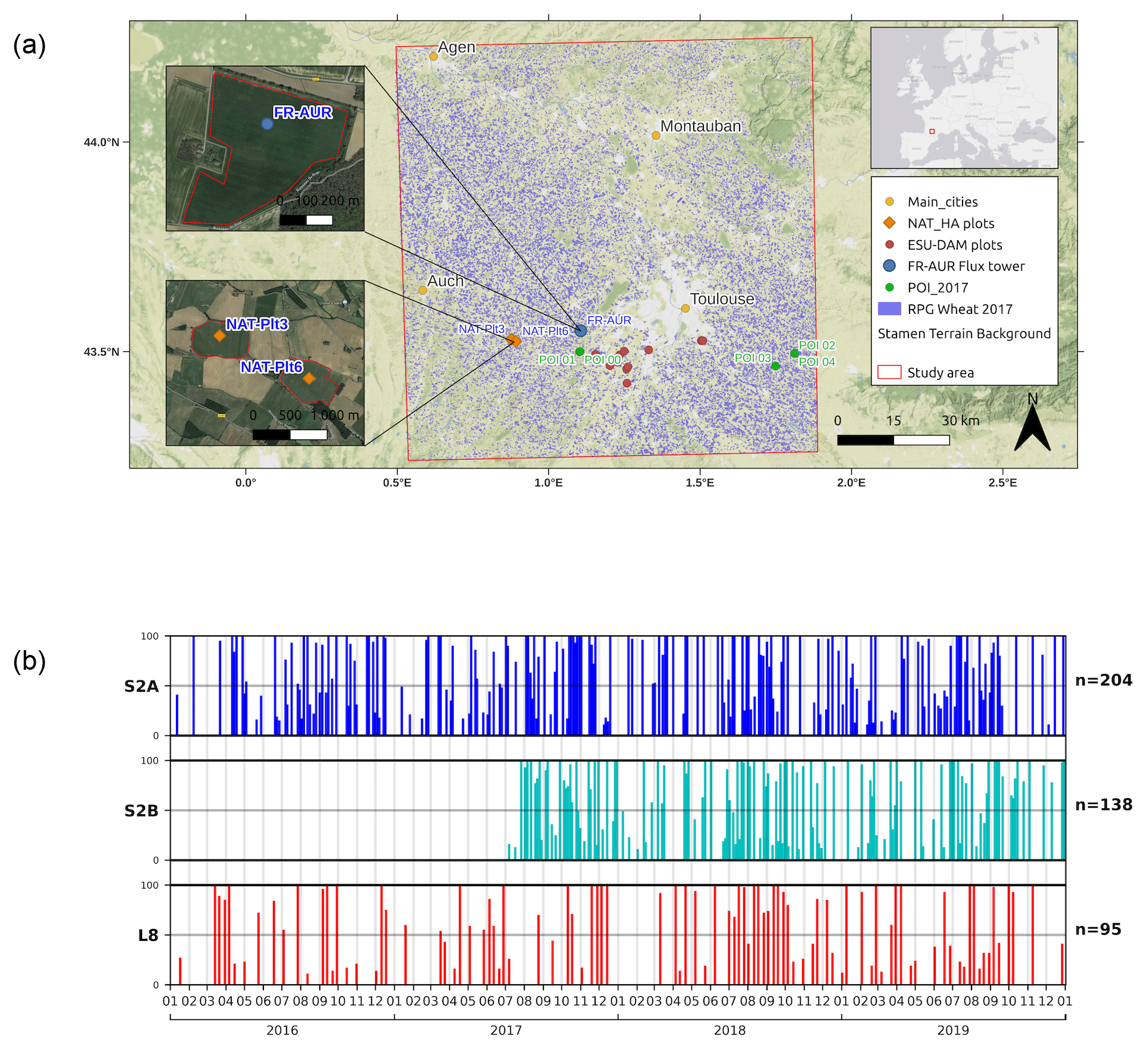
Figure 2 Map of the simulation area and image availability from 2016 to 2019. (a) Background the ESRI World Topo Map, the 31TCJ Sentinel2 tile limits (red rectangle), land cover for winter wheat fields for 2017 (blue), location of the FR-AUR ICOS site, the dry above-ground biomass (DAM) measurements (red circles) and the two fields monitored with connected combine harvesters (CHs) (orange circles). The zoomed maps show the FR-AUR field and the fields monitored using combine harvesters. (b) Chronogram of the remote sensing dataset from Sentinel-2A (S2A), Sentinel-2B (S2B), and Landsat-8 (L8), over the 31TCJ tile for 2016 to 2019. The bar plots represent the percentage of cloud-free pixels for each image.

Table 3 Name, aim, and input details of the assimilation experiment.

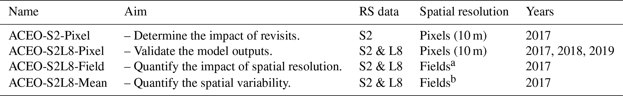
^a For ACEO-S2L8-Field the GLAI from PROSAIL inversion is averaged prior to the SAFYE-CO2. ^b For ACEO-S2L8-Mean the outputs at 10 m from SAFYE-CO2 are averaged at field scale.

The study area has a mean annual precipitation of 655 mm and a mean annual temperature close to 13 ^∘C. It is classified as a majorly temperate oceanic climate (Cbf) in the plains and temperate continental climate (Dfb) near the Pyrenees mountains, based on the Köppen climate classification. In 2017, winter was exceptionally dry and sunny, and spring was sunny, with a 10 % deficit in rainfall (Météo-France, 2019), while 2019 had a mild winter and a sunny spring, with 10 % deficit rainfall for the two seasons (Météo-France, 2021). The region has an intermediary cloud coverage that allows for multitemporal optical remote sensing analysis and analysis of the impact of clouds (Fig. 2b). It is mainly occupied by agricultural fields that cover approximately 90 % of the area, among which the majority is seasonal crops. Winter wheat covers approximately 20 % of the zone and reaches 40 % in some areas. In southwest France, soft-wheat varieties are predominant, and they are usually sown in autumn around the middle to the end of October. Soft wheat represents 75 % of the French exports of soft wheat. The crop typically develops slowly during the winter, and growth accelerates during spring. It is harvested from mid-June to the end of July depending on maturation as well as climatic conditions to optimize grain. The harvest in 2017 was normal (6 t ha⁻¹ at 15 % humidity), while 2019 was an exceptional year with a yield of 11.5 t ha⁻¹ at 15 % humidity (ARVALIS, 2019). In terms of pedology, two main soil types are present in the area of study: silt-rich soils near the major streams and clay soils across the hills with a variable density of stones depending on erosion. The topography offers a wide range of aspects. The region also bears the effects of historical land management, specifically, the “remembrement” policy, a political push to merge adjacent fields from 1945 to 1980 in France (Baker, 1961). This leads to a wide range of soil and microclimatic conditions that cause significant intrafield plant growth variability.

This study area was chosen for three main reasons in light of the aims of the paper. First, it is part of the Space Regional Observatory that benefits from extensive datasets regarding crop growth and crop physiology through the presence of two certified ICOS flux sites (FR-AUR and FR-LAM), and extensive measurement campaigns operated by different public laboratories specializing in agronomy and remote sensing as well as measurement campaigns operated by private companies and individual farmers. These measured variables related to the field's carbon budget such as NEE, GPP, R_eco, DAM, and yield (Eqs. 1 and 9) are monitored in different localities with different representative scales (Table 3.2). Second, the crop growth and biophysical process variability, due to topography and pedo-climatic variations, is needed to assess the impact of using high-resolution modelling and assimilation schemes in quantifying the carbon budget components (e.g. Yield, CO₂ fluxes). Third, winter wheat is one of the most studied crops worldwide. This allows us to compare the quality of the results obtained with AgriCarbon-EO against a large corpus of published studies. Furthermore, the area is a dense crop production zone. This is especially true for wheat production, which has a large economic interest.

3.2 Validation of the AgriCarbon-EO outputs

The validation relies on several datasets corresponding to the main output variables of AgriCarbon-EO: CO₂ flux measurements (i.e. NEE, GPP, R_eco), DAM measurements over elementary sampling units (ESUs), and yield maps. A summary of the ID and characteristics of the aforementioned validation datasets is presented in Table 4.

Table 4 Description of the validation data sets.

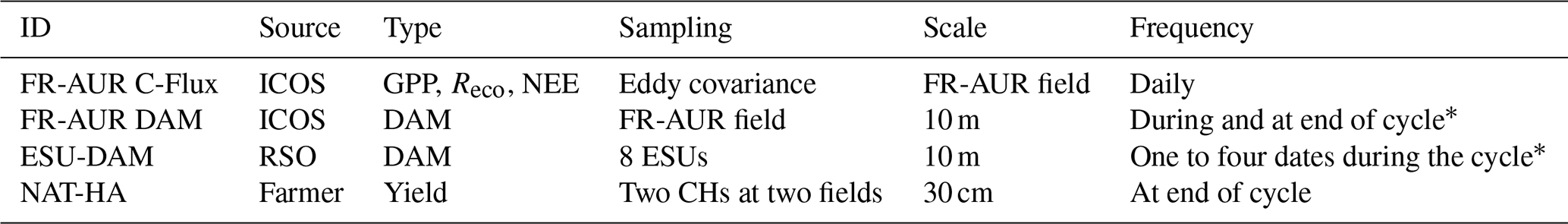
^* The list of dates is provided in the Supplement.

The validation datasets were extracted from the database of the Environmental Information System maintained by the CESBIO laboratory (SIE, 2022).

3.2.1 Validation against field-scale CO₂ fluxes and DAM measurements

The FR-AUR ICOS site provides many biophysical measurements, among which there are variables of interest regarding the carbon budget GPP, R_eco and NEE (FR-AUR C-Flux, Table 4). These variables allow us to assess the soundness of the representation of CO₂ fluxes caused by physiological processes in the model, as GPP represents photosynthesis and R_eco the sum of plant and soil respiration. NEE allows access to the representation of the biological part of the carbon budget. Furthermore, DAM is linked to carbon export (Eq. 9) and NPP (Eq. 1). As one of the requirements for the ICOS certification is the homogeneity of the ecosystem, the measurements were considered to be representative of the field. The DAM and CO₂ flux measurements were acquired using the ICOS destructive biomass sampling protocol (Gielen et al., 2018) and eddy covariance (EC) flux tower measurements processed with EdiRe software (Clement, 2008), following the CarboEurope-IP recommendations for data filtering, quality control, and gap filling (Table 4). The EC method consists of measuring the 3D wind fluctuations at 20 Hz using a high-frequency sonic anemometer and the CO₂ concentration using a gas analyser. The covariance is then computed between the turbulent component of the vertical wind and the turbulent component of the CO₂ concentrations (Baldocchi, 2003). The NEE was then partitioned into GPP and R_eco using a formulation for croplands in Béziat (2009) adapted from Reichstein et al. (2005). Depending on wind speed and the intensity of the turbulence, a fraction of the direct measurements are not representative of the plot, and those data points were filtered out during the processing and replaced with simulated values extrapolated from the environmental conditions. We maintained only daily data points where more than 50 % of the information comes from real measurements, as gap-filling over long periods induces high errors (Béziat, 2009). The days when less than 50 % of the information is provided by measurements are represented in grey in Fig. 3. Furthermore, it is also noticeable that the observed R_eco in 2018–2019 dips to zero during the vegetation growth period, which is related to an error in the partitioning process of NEE into GPP and R_eco. This period is also ignored for GPP and R_eco and is represented in red in Fig. 3.

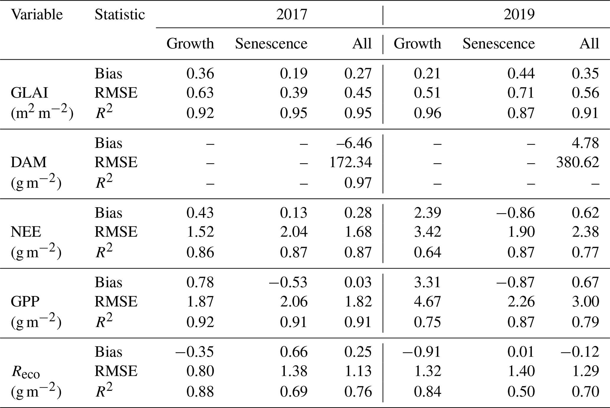
In this exercise, the daily outputs from AgriCarbon-EO at 10 m resolution were spatially averaged over the area of the FR-AUR field (Eq. 14) sampled by the EC tower (a.k.a. the target area in the ICOS nomenclature). Those averaged values were then compared against FR-AUR DAM and FR-AUR C-Flux as shown in Fig. 3, and the corresponding fitting statistics are shown in Table 5. The statistics were computed for three specific periods, from 1 January to 1 May, 1 May to 1 July, and 1 October to 1 October. These periods correspond to the growing and senescence of the wheat crop and the whole cropping year respectively. The GLAI fitting statistics computed over the growing season show a good fit (R²=0.95) in 2016–2017 with a slightly lower fit in 2018–2019 (R²=0.91). From mid-November 2018 until the end of January 2019, spontaneous regrowth of the previous crop (i.e. rapeseed) was observed in the field. The model does not reproduce this GLAI dynamic, as this increase does not correspond to the wheat crop cycle. The GLAI for the 2018–2019 senescence period is underestimated by the model.

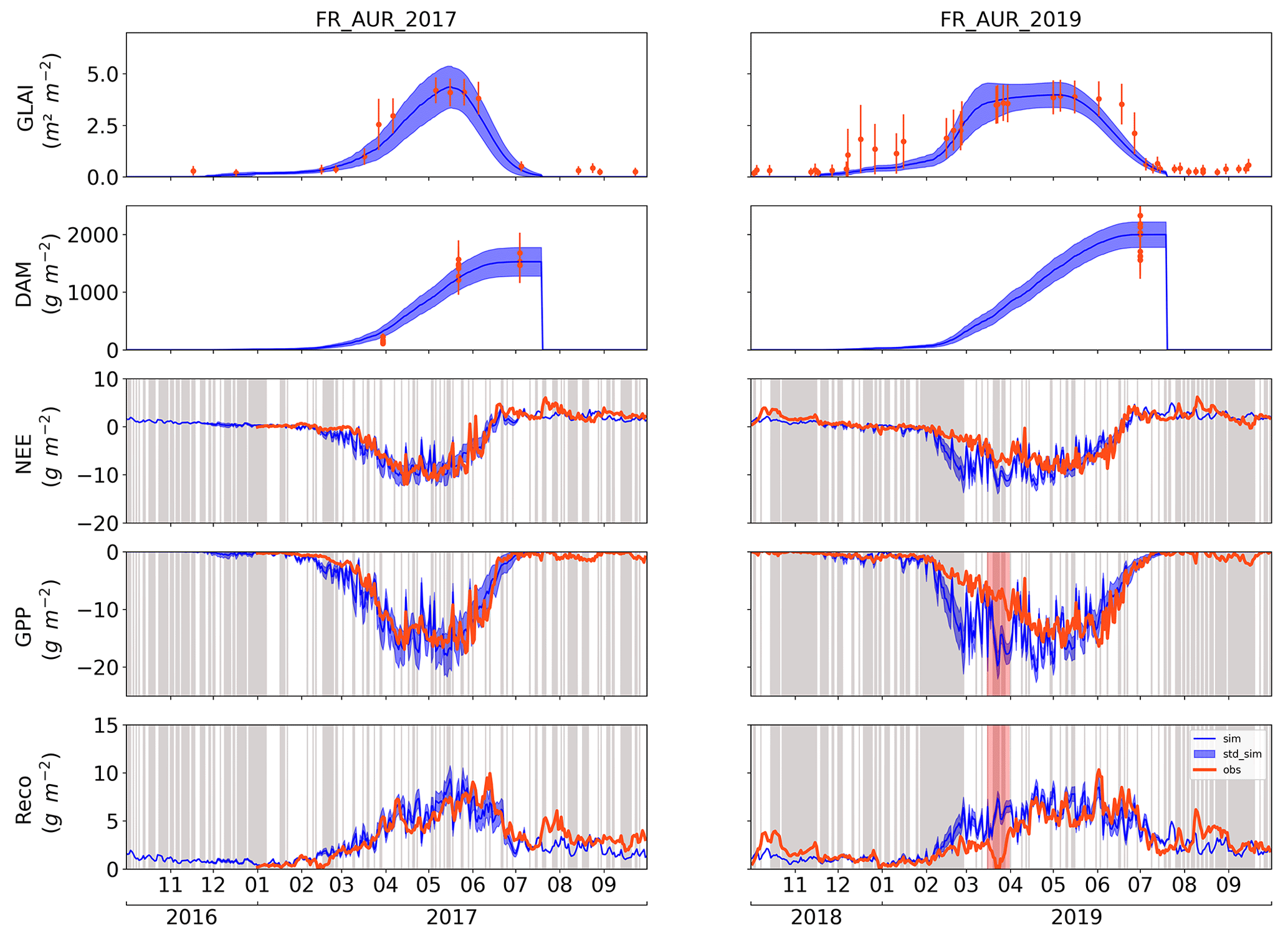
Figure 3 Time series of GLAI, DAM, NEE, GPP, and R_eco. The blue line and surface represent the mean and standard deviation of the posterior distribution. The orange points with error bars represent the GLAI derived from the satellite observations and the DAM, NEE, GPP, and R_eco at the FR-AUR site for 2 cropping years (2016–2017 and 2018–2019). In the case of the CO₂ fluxes, the grey areas represent the days during which more than 50 % of the data are gap-filled, and the red area represents the periods during which a partitioning error has been identified.

Regarding observed as well as simulated DAM, end-of-cycle values are higher for the 2019 cropping year than in 2017, which is consistent with regional yield statistics (ARVALIS, 2019). Additionally, the modelled above-ground-biomass dynamics are consistent with the observed dynamics, apart from an overestimation of the simulation at the beginning of the vegetation cycle in 2017. Note that replicates in 2016–2017 and 2018–2019 present a noticeable spread. In 2017, the dynamics of the CO₂ fluxes are well represented, with most of the observed values in the uncertainty margin of the model, with R² values of 0.87, 0.91, and 0.76 for NEE, GPP, and R_eco, respectively. The model's daily flux variations are slightly higher than the observations in 2017. In 2019, the CO₂ flux dynamics are less well reproduced, nevertheless with acceptable R² values (above 0.7) over the full year. For the cropping year, R² was 0.77, 0.79, and 0.70 for NEE, GPP, and R_eco respectively. The modelled GPP values are significantly higher than the observed values during the growing period (bias =3.31 gC m⁻²), while the differences between the model and observations are less pronounced at the end of the vegetation cycle (bias $=-\mathrm{0.87}$ gC m⁻²).

Table 5 Bias, R², and RMSE statistics for GLAI, DAM, GPP, R_eco, and NEE variables in FR-AUR site over years 2017 and 2019 for the growth and senescence and cropping year.

3.2.2 Validation against spatialized DAM measurements

The ESU protocol allows the assessment of variables at decametric scales. Among those variables, DAM is especially of interest as it can be used as a proxy for NPP (Eq. 7). Moreover, the exported yield can be computed using end-of-cycle biomass (Eq. 9). To measure DAM with the ESU protocol, the above-ground vegetation is sampled at five points following a cross pattern inscribed in a 10 × 10 m square; each sample corresponds to 1 linear metre of the crop row. The five samples are weighed fresh in the field. In the laboratory, one of the five samples is dried to retrieve the canopy water content, which is then applied to the five fresh weight measurements to obtain dry above-ground biomass. The mean and standard deviation are computed to obtain a representative DAM (g m⁻²) for the ESU. Eight fields were sampled using the ESU protocol in 2018, and simulations were performed for each ESU (Supplement).

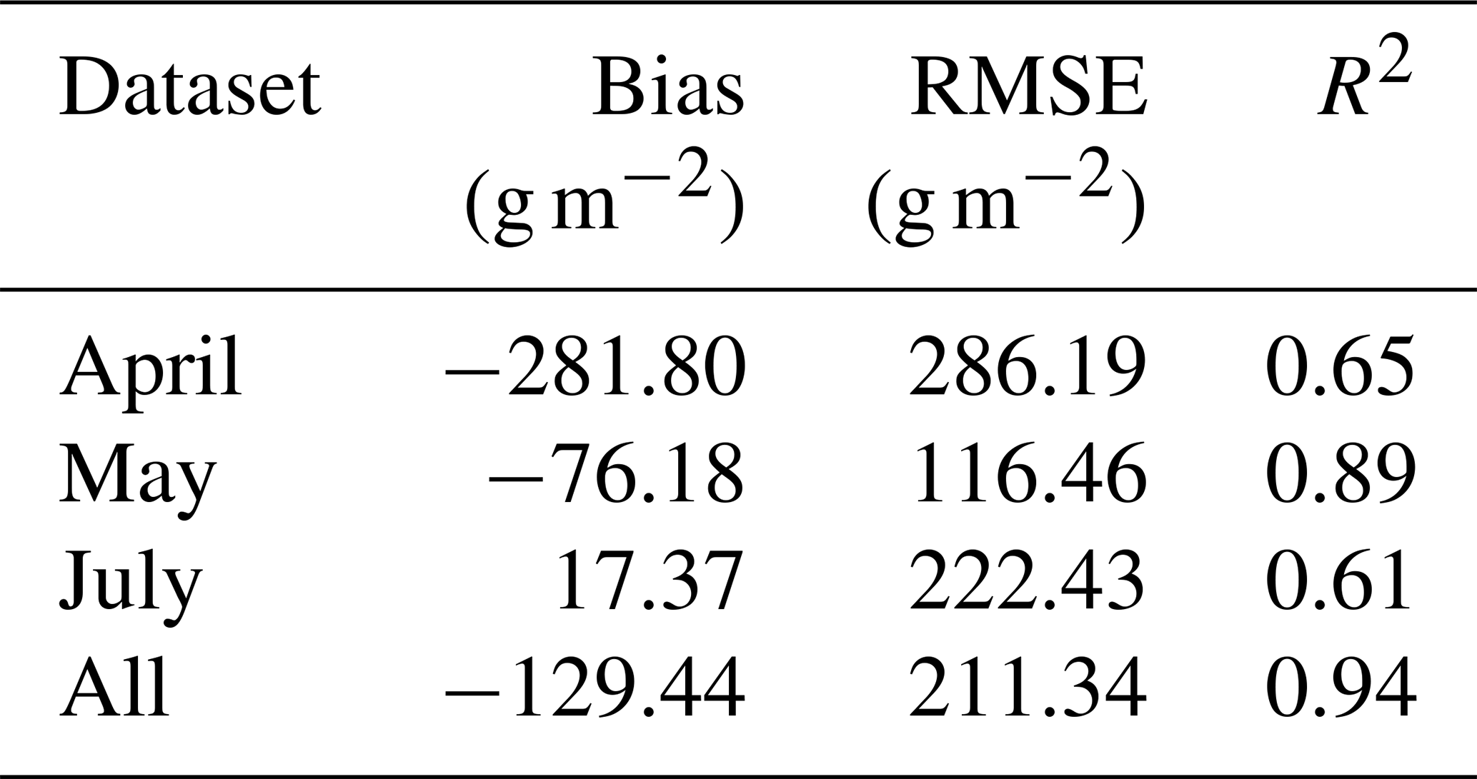
Figure 4 shows the scatter plot between the simulated and observed DAM coloured with respect to the month of acquisition for eight fields with up to four revisits. The statistics corresponding to this figure are recorded in Table 6. The comparison shows a good fit when considering all DAM measurements, with an R² of 0.94, an RMSE of 211.34 g m², and a mean overestimation of the model of 129 g m⁻². These statistics represent the spatiotemporal fitting of the model.

When analysing the statistics per month, it is noticeable that most of the total bias is present at the early growth stages (in April), and the bias decreases over the growing season. The final DAM values linked to yield and carbon exports in July have low bias, and we can explain 61 % of the variability. In addition, a weaker correlation is present when the data are split per month compared to the full dataset (Table 6). The variability in a given month is mainly due to the spatial variability. Splitting the data thus enables us to assess the variability in the spatial and temporal components that are simulated by AgriCarbon-EO. Given the small sample size, these monthly results should be interpreted with caution.

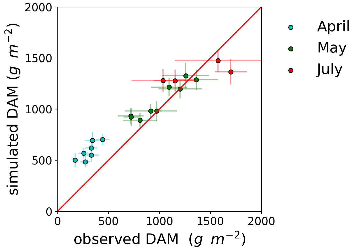
Figure 4 Scatter plot of the simulated winter wheat dry above-ground biomass (DAM) versus the observed biomass in the fields in 2018.

Table 6 Values of RMSE, MAE, bias, and R² between the simulated and observed dry above-ground biomass (DAM).

3.2.3 Comparison with high-resolution combine harvester yield maps

Yield maps are of high interest for the evaluation of high-resolution crop models in the context of carbon and precision farming. They provide information on the grain yield that often represents the bulk of the carbon that is exported from the field. CHs are also the only readily available spatial and direct high-resolution crop organ monitoring tools. Nevertheless, they have drawbacks because the mass flow sensor and the grain moisture content sensor can experience significant sensor drift within the field. Moreover, CH yield data processing requires a range of parameters such as lag time settings and distance travelled via GPS measurements, header position, and cut width, all of which contribute to the uncertainty in the measurements (Grisso et al., 2002). In this study, yield CH data were provided by a farmer located in the Gers département. Data from two fields NAT-Plt3 and NAT-Plt6 (Table 4), were collected by a CH that measures the incoming flow of grain, its humidity, and its position at a fixed frequency with a GPS. These measurements were integrated between two points of the trajectory taking into account harvesting width to compute the grain production (yield) per surface area. The grain humidity content enabled the computation of the dry yield mass (g m⁻²). The point yield data are then converted into a harvest map over the simulation grids by summing the points inside each pixel. A Gaussian smoothing filter with sigma =12 m was then applied over these maps to reduce the aliasing effects. The spatial anomaly (i.e. $(\mathrm{value}-\mathit{\mu })/\mathit{\sigma })$ maps were also computed. To complete the processing, the co-localization error between observations and AgriCarbon-EO yield estimates was minimized through the detection of the maximum spatial correlation in a 10 m lateral shift range.

The simulated yield maps were obtained from the ACEO-S2L8-Pixel simulation by multiplying the final DAM by HI (Eq. 9). We analysed the results in terms of the retrieval of the spatial patterns as shown in Fig. 5. These maps show the comparison between the CH yield data and the AgriCarbon-EO yield estimates at the pixel level (in t ha⁻¹) as well as the spatial yield anomaly. Overall, the observed yields show a larger variability than the simulations, and a clear saturation effect is observed in the simulations for the NAT-plt6 field. The AgriCarbon-EO and CH anomaly maps show clear spatial patterns. However, the spatial patterns are more pronounced over the NAT-Plt3 field than over NAT-Plt6. RMSEs of 0.70 and 0.68 t ha⁻¹, biases of 0.42 and 0.41, and R² values of 0.12 and 0.29 are observed for NAT-Plt3 and NAT-Plt6, respectively. The performances of the yield simulations vary strongly between the two fields. A relatively low RMSE and bias indicate a quite good mean representation of the plots. However, the correlation coefficient is quite low and indicates that not all the spatial variability in yield can be captured using this approach. The small R² can however be explained by the range of variation in wheat yield that is smaller at the intrafield scale than regional scale. Maximum R² values for these datasets are found to be respectively 0.32 and 0.22 when assuming an observation measurement error of 1 t ha⁻¹ (Supplement). Furthermore, if we compare these simulations to standard field-wise simulations that do not explain spatial variability, the explained spatial variance illustrated here is a net gain. Difficulties in reproducing the range of yield observed variations in yield values may be caused by the simple representation of grain biomass allocation through the use of an HI which does not take into account potential variations in the HI due to nutrient availability or crop cycle duration (Dai et al., 2016).

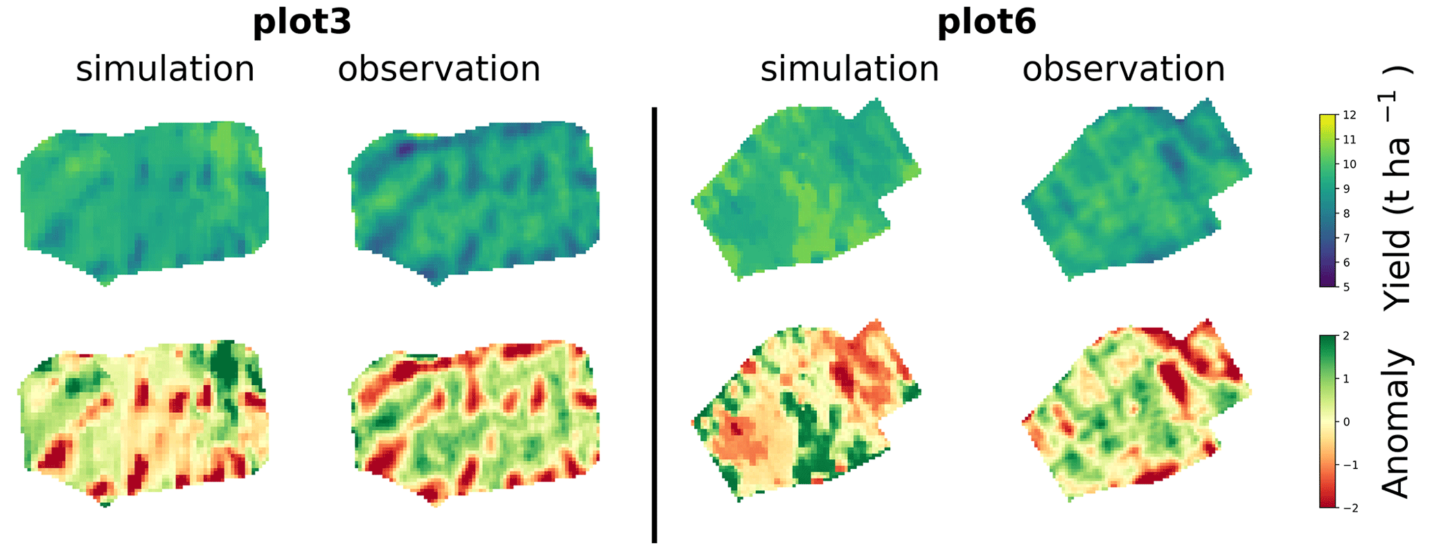
Figure 5 Yield maps and spatial anomalies simulated by AgriCarbon-EO and collected using a combine harvester over the Nataïs site (NAT-Plt3 and NAT-Plt6) for 2017 and 2019.

3.3 Large-scale simulation outputs

In this section, the results from the ACEO-S2L8-Pixel in 2017 are illustrated and analysed. The RPG land cover map for winter wheat fields, the SAFRAN weather data, and the THEIA S2 and L8 EO data were used as input along with the parametrization files for PROSAIL and SAFYE-CO2. The AgriCarbon-EO processing chain was run in parallel over a single server rack with two computation nodes and with 36 threads maximum. The memory requirement was the highest for the PROSAIL retrievals, reaching 5 GB per process (image inversion) for a LUT size of 5000. For SAFYE-CO2 the requirements were 5 GB per process, with one process per node of the weather grid with a LUT size of 5000. A SAFYE-CO2 run over the 110 × 110 km area of study at 10 m resolution required 4 h of computation time per year of simulation. The chain was able to produce maps of all parameters and variables estimated by SAFYE-CO2. With the carbon budget being our main priority here, we chose to focus on NEP, DAM at the end of the vegetation cycle, Cexport (Eq. 9), and NECB (Eq. 1). NEP was computed by summing NEE over 1 cropping year from 1 October 2016 to 30 September 2017. Maps of NEP, Cexport, and NECB at native resolution (10 m) are shown in Fig. 6a as an illustration of typical outputs from the chain. The histograms of the same variables and their uncertainty are shown in Fig. 6b. Note that, in these figures, we presented NEP and NECB in the soil-oriented convention (i.e. positive values mean net CO₂ fixation and soil organic carbon storage, respectively) to be able to compare the values of NEP, Cexport, and NECB.

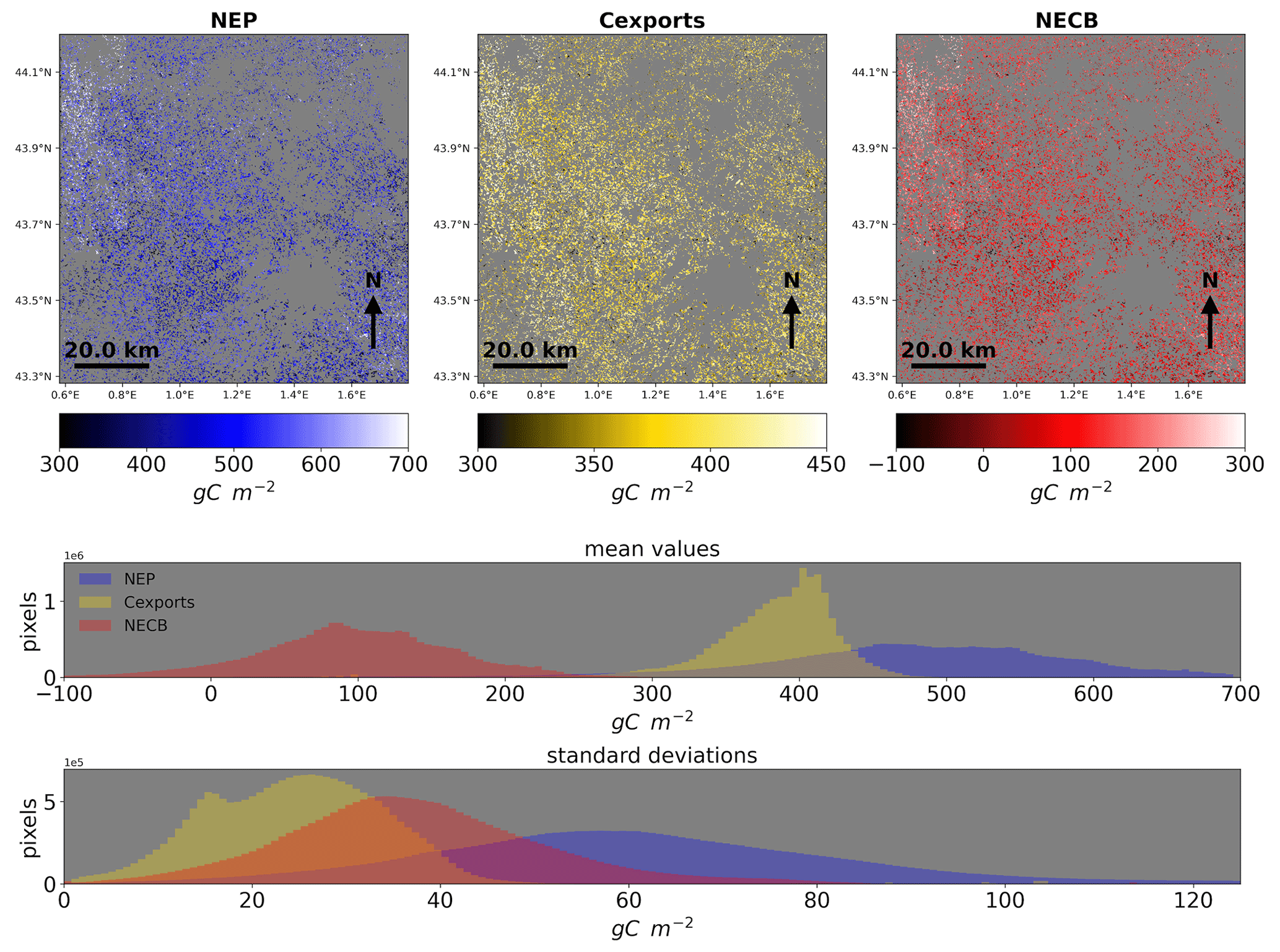
Figure 6 Regional-scale carbon budget outputs from AgriCarbon-EO assimilation using S2 and L8. (a) From left to right, NEP, Cexport (yield), and NECB for the winter wheat fields for the 2016–2017 cropping season. In (b) the histogram of the posterior mean and standard deviation of the same variables on top and bottom, respectively. Note that NEP and NECB are presented in the soil-oriented convention. Positive values of NEP and NECB thus correspond to net annual CO₂ sinks and soil organic carbon storage, respectively.

High levels of heterogeneity with regional patterns can be seen in the retrieved simulations. The northwestern and southeastern corners are characterized by higher CO₂ fixation and thus growth, yield, and lower NECB. The variability of NEP is mostly comprised between 300 and 700 gC m⁻², which is consistent with eddy covariance measurements for wheat across Europe (Ceschia et al., 2010). Furthermore, the dry yield varies between 6.6 t ha⁻¹ (i.e 300 gC m⁻²) and 10 t ha⁻¹ (i.e. 450 gC m⁻²), which is also coherent with regional statistics (ARVALIS, 2019). In Fig. 6, negative values of NEP and NECB correspond to pixels where wheat did not develop. In those cases, Rh dominates during the cropping year, leading to a net carbon loss in the soil.

The uncertainty (i.e. standard deviation of the posterior distribution) has mean values of 55, 25, and 38 gC m⁻² for NEP, Cexport, and NECB, respectively. The spatial variability (i.e. standard deviation of the mean pixel values) is equal to 131, 50, and 82 gC m ⁻² for those same variables. The fact that the uncertainty is lower than the retrieved spatial variability indicates that this method has enough resolution to discriminate and ordinate values of NEP, Cexport, and NECB based on the update of priors using remote sensing-based GLAI. However, the fact that those values are on the same order of magnitude stresses that uncertainty assessments should always be provided with these analyses. The maps and distributions, given their scale and resolution, do not showcase the full range of crop variability that can be observed in the study area. To illustrate individual solutions and anomalies encountered in the simulations, selected pixels of interest (POIs; located in Fig. 2) are presented in Fig. 7.

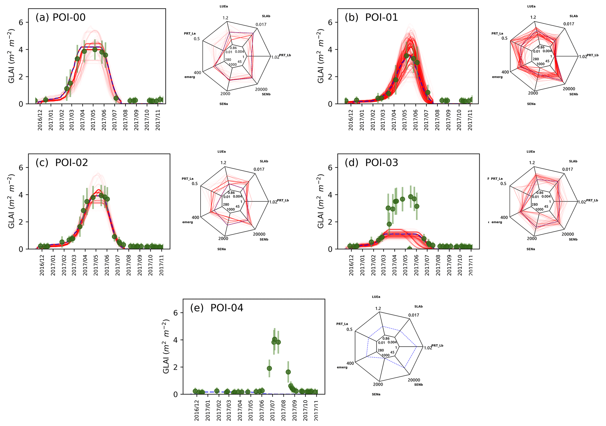
Figure 7 Time series of GLAI and radar plots containing the free parameters of SAFYE-CO2. Simulations are represented in red with a transparency proportional to their relative likelihood, and the maximum likelihood simulation is represented in dashed blue lines. POI-00 (a) and POI-01 (b) are located in the same field. POI-02 (c) and POI-03 (d) are adjacent pixels where a cloud date is not filtered in (d). POI-04 (e) illustrates either an error in the CAP declaration or a failed wheat crop followed by a summer crop.

These pixels are selected to illustrate intrafield heterogeneity and specific anomalies. Figure 7a–e show the GLAI inverted using PROSAIL in green with their respective uncertainties and the simulated GLAI time series in red, with higher transparency for the solutions with the lowest contribution (likelihood). For instance, the results in Fig. 7a POI-00 and Fig. 7b POI-01 show the fitting of the model over 2 pixels in the same field. It is clear from the observed and the GLAI between the two POIs that the vegetation phenology is different, with early emergence and higher maximum GLAI in the case of POI-00 (Fig. 7a) and later emergence and lower maximum GLAI in the case of POI-01 (Fig. 7b). Additionally, Fig. 7c POI-02 and Fig. 7d POI-03 are adjacent pixels in the same field, but each is on a different side of a cloud mask in May 2017. The input GLAI from PROSAIL on this date is associated with very low uncertainty, which impacts the retrieval of the SAFYE-CO2 model. The low uncertainty will result in a high level of false information for this date, which in turn will negatively impact the Bayesian inversion and reduce the SAFYE-CO2 model performances, thereby pushing the model to better fit this unrealistic inversion of GLAI. Finally, Fig. 7e POI-04 corresponds to a pixel in a field where the observed GLAI is not consistent with winter wheat; in fact, this GLAI dynamic fits better to a summer crop such as sunflower. Mislabelling in the land cover such as this one can result in “no fitting”. Mislabelled winter crops could, however, be fitted and not stand out in the spatialized simulation.

3.4 Impact of the spatial resolution and temporal sampling of assimilated GLAI

The AgriCarbon-EO simulations (Table 3) were compared at different scales (i.e. pixel vs. field) and for different satellite image temporal densities to investigate the benefit of assimilating high-resolution multimission-derived GLAI into SAFYE-CO2. The impact of the spatial scale of the GLAI assimilation is illustrated by Fig. 8a, which shows the histogram of DAM${}_{\mathrm{ACEO}-\mathrm{S}\mathrm{2}\mathrm{L}\mathrm{8}-\mathrm{Pixel}}-$ DAM${}_{\mathrm{ACEO}-\mathrm{S}\mathrm{2}\mathrm{L}\mathrm{8}-\mathrm{Field}}$. An average negative bias of −47 g m⁻² is observed for DAM with a spread between −210 and +120 g m⁻² for the $[-\mathit{\sigma },+\mathit{\sigma }]$ interval when comparing the pixel-scale simulation to the field-scale simulation. This result is interpreted as the bias error that can be avoided by applying an intrafield assimilation scheme in the crop model in contradiction to the more generally applied field scale. Note that the same bias value is obtained for Fig. 8b, representing the difference between the averaged pixel at field scale and the field-scale simulations: DAM${}_{\mathrm{ACEO}-\mathrm{S}\mathrm{2}\mathrm{L}\mathrm{8}-\mathrm{Mean}}-{\mathrm{DAM}}_{\mathrm{ACEO}-\mathrm{S}\mathrm{2}\mathrm{L}\mathrm{8}-\mathrm{Field}}$. This is mathematically expected as DAM${}_{\mathrm{ACEO}-\mathrm{S}\mathrm{2}\mathrm{L}\mathrm{8}-\mathrm{Mean}}$ is obtained by averaging the DAM${}_{\mathrm{ACEO}-\mathrm{S}\mathrm{2}\mathrm{L}\mathrm{8}-\mathrm{Pixel}}$ simulations. However, when comparing the RMSE values between Fig. 8a and b, a noticeable change in RMSE of −68 g m⁻² is observed. This result shows that the variability of simulated biomass will decrease by 39 % when considering field-scale modelling. The variability is directly influenced by the retrieved parameters of the crop model between the intrafield and field scales for the same crop cycle, resulting in a different posterior parameter distribution, as shown in the section above. Figure 8c shows the difference between a simulation using only S2 and using S2 + L8. Adding L8 images tends to slightly increase dry biomass, with a bias of 30 g m⁻² and an RMSE of 94 g m ⁻². This difference is caused by the additional samples added at the start and end of the vegetation cycle that result in a change in the length of the vegetation cycle. To assess the robustness of the assimilation approach with respect to the number of assimilated images, the DAM outputs from ACEO-S2L8-Pixel were analysed in terms of the number of images over each pixel. Figure 9 shows the impact of the number of GLAI observations per pixel on μ and σ of the DAM. σ of DAM decreases by approximately 66 % with the number of observations (146 g m⁻² for 11 images to 48 g m⁻² for 28 images), while the μ DAM values remain stable. This illustrates the stability of μ values given the range of variation of observed images. However, the decrease in σ also illustrates the contribution of the number of images to the constraining of solutions and increased accuracy.

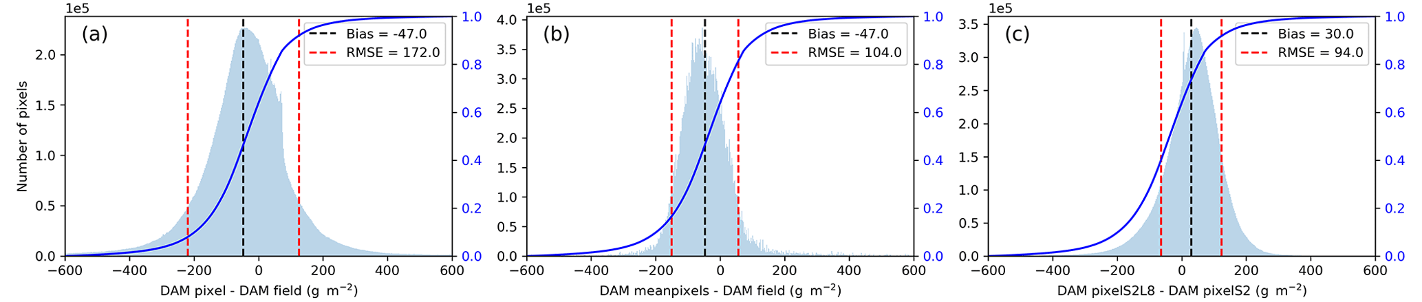
Figure 8 Histogram (left y axis) and cumulative density function (right y axis) of the bias of biomass at harvest (y axis). Panel (a) corresponds to DAM${}_{\mathrm{ACEO}-\mathrm{S}\mathrm{2}\mathrm{L}\mathrm{8}-\mathrm{Pixel}}-{\mathrm{DAM}}_{\mathrm{ACEO}-\mathrm{S}\mathrm{2}\mathrm{L}\mathrm{8}-\mathrm{Field}}$, panel (b) to DAM${}_{\mathrm{ACEO}-\mathrm{S}\mathrm{2}\mathrm{L}\mathrm{8}-\mathrm{Mean}}-{\mathrm{DAM}}_{\mathrm{ACEO}-\mathrm{S}\mathrm{2}\mathrm{L}\mathrm{8}-\mathrm{Field}}$, and panel (c) to DAM${}_{\mathrm{ACEO}-\mathrm{S}\mathrm{2}\mathrm{L}\mathrm{8}-\mathrm{Pixel}}-{\mathrm{DAM}}_{\mathrm{ACEO}-\mathrm{S}\mathrm{2}-\mathrm{Pixel}}$.

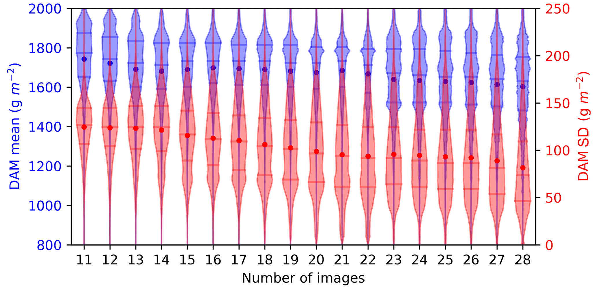
Figure 9 Violin plots of the number of images used for the inversion over each pixel on the x axis and the mean (μ) DAM on the right y axis and the standard deviation (σ) of DAM on the left y axis.

4 Discussion

4.1 Accuracy of carbon budget component retrieval

The performances of our retrievals of the carbon budget components are put here in the context of relevant studies. In the previous applications of SAFYE-CO2, Pique et al. (2020a) implemented an iterative retrieval algorithm at the field scale. This algorithm is not scalable for intrafield simulations at the regional scale, and it does not provide an estimate of the associated uncertainty. Their validation exercises for wheat with SAFYE-CO2 over the FR-AUR flux tower showed R² ranges of [0.78,0.90], [0.82,0.94], and [0.58,0.84] for NEE, GPP, and R_eco, respectively. The results from our study are in the same ranges, considering the two studies address different years and different EO data: [0.77,0.87], [0.82,0.87], and [0.7,0.76] for NEE, GPP, and R_eco, respectively. The implementation of the BASALT algorithm, while enabling uncertainty estimates for regional-scale applications, does not come at the expense of the accuracy of the retrievals. Other studies addressed the estimates of NEE and GPP. Combe et al. (2017) constrained the WOFOST agronomic model at 25 km resolution using yield and sowing dates, over three ICOS sites and 10 site years. They obtained R² values of [0.64,0.74] and RMSE values of [2.33,2.67] g m⁻² for NEE over wheat fields. The values we retrieved for FR-AUR are better regarding R² [0.77,0.87] and RMSE [1.68,2.36]. Combe et al. (2017) also obtained R² and RMSE values of [0.82,0.87] and [2.33,2.83] g m⁻² for GPP, respectively. The R² retrieved from AgriCarbon-EO is slightly higher [0.82,0.87], and the RMSE was in the same range for 2019 and lower for 2017. R_eco is not systematically addressed in the modelling exercises, as it requires simulation of the plant and soil processes simultaneously. Combe et al. (2017) retrieved R_eco with R² values of [0.76,0.83] and RMSE values of [0.98,1.29] g m⁻². The R² obtained with AgriCarbon-EO is slightly lower [0.70,0.76] and the RMSE slightly higher [1.13,1.29] g m⁻²) than in Combe et al. (2017) for R_eco. The R_eco estimates depend on Rh and R_auto. We recommend that Rh should be enhanced using a more complete soil module. This point is addressed later in this discussion. In addition to NEE, GPP, and R_eco, the other components of the carbon budget involve the biomass and yield estimates that are either exported out of the field or integrated into the soil. Tewes et al. (2020) assimilated in situ LAI into the LINTUL5 crop model using NIS. Their DAMs at maturity (BBCH 99) were compared against field measurements collected on 14 plots in the Netherlands, northern France, and Germany (from 40 to 60 in situ points over 1 m²), showing a mean RMSE of 246 g m⁻² and a mean bias of 58 g m⁻². The end-of-cycle biomass retrieved using AgriCarbon-EO shows similar performances (RMSE =222 g m⁻² and Bias =17 g m⁻²) while using GLAI derived from satellite measurements (see Table 6). Hao et al. (2021) presents a meta-analysis of 76 studies using the APSIM model, which is broadly used for wheat yield simulations. They find that an RMSE =100 g m⁻² is expected for applications of this model. The RMSE retrieved by AgriCarbon-EO is in the same order as these studies (RMSE =60–70 g m⁻²). While the estimates are reasonable, we consider that the use of a direct harvest index to determine yield may present some limitations, more so in the presence of extreme events during the grain filling. Our bibliographical research yielded no other studies that perform crop growth simulations and estimation of the carbon budget components at a decametric resolution while covering very large areas. Most of the studies perform low-resolution analysis in plains, where the spatial variability is expected to be low. The same approaches may be penalized when applied to areas with high spatial variability, such as the hilly countryside in southwestern France. When compared to existing studies, we find that AgriCarbon-EO allows the retrieval of the main carbon budget components with performances that are close to or better than existing state-of-the-art evaluations. An extended application of AgriCarbon-EO over a variety of pedo-climatic conditions by taking advantage in particular of the data provided through the regional Fluxnet, ICOS, and Ameriflux networks will help in confirming this statement.

4.2 Multi-mission data, cloud cover, and limitations

The retrieval of SAFYE-CO2 parameters and the carbon budget components in AgriCarbon-EO relies on the accuracy and availability of EO data, which can be hampered by errors in image co-location, atmospheric corrections, the presence of clouds, and cloud shadow correction. Many studies show that these effects have an important impact on agricultural remote sensing applications, such as yield estimation (Soriano-González et al., 2022), land cover (Song et al., 2021), and superficial soil carbon content mapping (Vaudour et al., 2019). While we find that these effects are in the large majority mitigated through the use of a Bayesian approach for the GLAI assimilation, we identified examples where the retrieval of GLAI is associated with a low uncertainty when clouds or cloud shadows persist. Unfiltered clouds or the lack of images can significantly impact the simulations locally (Fig. 7c). Consequently, the analysis of GLAI time series to detect anomalous variations (Fig. 7d) or improvements in cloud detection algorithms like in Skakun et al. (2022) would improve GLAI inversions in AgriCarbon-EO. The use of additional data from L8 with a coarser spatial resolution than S2 enhanced the simulation quality for our region of interest. The most notable impact was the reduction of uncertainty due to the increased constrained by the additional images. An additional option would be the use of daily high-resolution optical data from Planet Labs at <5 m. Still, there is a limit to the addition of optical images when clouds are persistent over long periods, which are most frequent in tropical areas. In these cases, the use of biophysical variables retrieved from Synthetic Aperture Radar (SAR) satellite data could mitigate the loss of data (Veloso et al., 2017; Fieuzal et al., 2017). This can be achieved through the relation between the above-ground biomass of crops and the radar polarization ratio or vegetation index (RVI). This would imply the use of a multi-variable assimilation scheme that considers GLAI from optical and DAM from SAR. This is feasible using the BASALT scheme in AgriCarbon-EO as the Bayesian assimilation algorithm can be easily adapted for multi-variable assimilation.

4.3 Impact of remote sensing and input spatial resolution

Intrafield heterogeneity is a well-established issue in agricultural applications (Weiss et al., 2020; Blackmore et al., 2003; Grieve et al., 2019; Nowak, 2021). However, it has not been thoroughly treated in terms of CO₂ fluxes and uncertainty estimates. In this paper, we argue that reliable and accurate estimates of DAM and CO₂ fluxes in support of carbon budget component monitoring require intrafield-scale estimates. Our results show that by assimilating mean-field-level GLAI products in SAFYE-CO2, a bias of −47 g m⁻² and an artificial relative uncertainty decrease of 39 % on DAM will be induced compared to assimilating high-resolution GLAI and calculating the mean of the model's output. The high spatial resolution thus allows more accurate estimates of the mean DAM values at the field scale, which in turn also enables more accurate field-scale estimates of SOC changes by soil models. Nevertheless, the use of even higher-resolution remote sensing data may be relevant to address carbon budget components at very small or elongated fields, such as those in rural India (Deininger et al., 2017). For example, current data at <5 m spatial resolution from Planet Labs, mentioned above, or future data from the next-generation (NG) Sentinel-2 constellation can extend the applicability of approaches like AgriCarbon-EO to small fields. The other input data products that drive the spatial resolution of the AgriCarbon-EO outputs are the land cover and the weather data. While the land cover is available at an adequate resolution (i.e. field scale), it is error-prone, either because of erroneous CAP declarations (Magnin, 2019) or because of classification errors when EO-based land cover maps are used (Liu et al., 2022). Interestingly, our results show that when a mismatch occurs, the fields in question exhibit high anomalies in retrieved parameters and are thus detectable. For the weather forcing, the current application was based on the Météo-France 8 km resolution Safran data, which provides reasonable accuracy over France (Garrigues et al., 2015). Currently, ECMWF provides ERA5-Land at 0.1^∘ resolution globally (Muñoz-Sabater et al., 2021), and NOAA provides weather reanalysis at 3 km over the US (Dowell et al., 2022). In the future, the coverage and resolutions of weather forcing data are expected to increase (i.e. ERA6 at 2.5 km). Increasing the resolution of the weather forcing in AgriCarbon-EO would provide better spatial information but would also increase the computational demand by a factor of γ as the LUT for SAFYE-CO2 is generated over the weather grid (Eq. 16).

$$\begin{array}{}\text{(16)}& \mathit{\gamma }={\displaystyle \frac{\mathrm{TLUT}\times {\mathrm{8}}^{\mathrm{2}}}{{\mathit{\theta }}^{\mathrm{2}}}}\end{array}$$

TLUT is the processing time for the generation of LUT, and θ is the weather grid resolution (in km).

4.4 Limitations of the Bayesian and physically based approach

While the components of AgriCarbon-EO have been tailored to the requirements mentioned in the Introduction (large-scale, high-resolution, uncertainty estimates, and biophysical processes), we have shown limits for each of them. For instance, the BASALT Bayesian approach can be sensitive to an erroneous observation associated with low uncertainty (Fig. 7d). A trade-off must be made between the range covered by the generated solutions and the number of LUT entries in order to maintain computational efficiency. A solution could be to consider a joint distribution for prior parameters to propose a better ratio of appropriate solutions (Wang et al., 2022). Another point is that the radiative transfer modelling is constrained by the spectral library database (Verhoef et al., 2007), which may not reflect ground conditions such as the presence of weeds impacting GLAI retrievals. Another limitation is that the crop model predictions require crop-dependent fixed and prior parameters. As an alternative solution to bypass some limitations, one could have reverted to machine learning approaches that have gained popularity for precision agriculture and soil carbon farming applications (Sharma et al., 2021). However, while they are powerful tools, they need a large amount of training data to take into account climatic conditions and management practices and need to be updated regularly as we encounter unprecedented weather conditions. Hybrid solutions such as AgriCarbon-EO that combine parsimonious process-based modelling and remote sensing approaches are thus needed. In the current state, it is reasonable to consider that an MRV platform for SOC carbon stock changes should include an ensemble of approaches with varying levels of complexity (e.g. Tier 1, 2 and 3) (Nevalainen et al., 2022), similar to what has been implemented in the IPCC approaches (Parker, 2013). In this framework, AgriCarbon-EO is designed to be a Tier 3 MRV approach for crop carbon farming.

4.5 From AgriCarbon-EO to SOC budget

The present approach provides high-resolution estimates of key carbon budget components and estimations of NECB and SOC variations. To achieve this, the SAFYE-CO2 crop model currently uses a simplified soil respiration module that simulates Rh that does not include the modelling of the processes in the different carbon pools in the soil (e.g. humification, mineralization) (Eq. 11). This methodology is adapted for the short-term assessment of carbon budgets (typically up to 1 year) (Pique et al., 2020a). This means that stock-dependent soil processes that affect SOC mineralization and litter humification that may cause priming effects are not accounted for here. The inclusion of a soil carbon decomposition module, as in Guenet et al. (2016), that includes such processes would allow a better representation of soil respiration and account for the effect of amendments with different decomposition dynamics. Such an exercise, would, however, increase the number of parameters and create the need for the addition of in situ or spatial maps to provide initial soil carbon content, soil chemical characteristics, and organic amendment information. Procurement at a large scale of such information with sufficient accuracy is still challenging for large-scale applications. One way of achieving this is to take advantage of the rapidly developing Farm Management Information Systems (FMIS) and enhanced soil property maps through digital soil mapping (DSM). Even though farmer activity data are not easily accessible, it is expected that this limitation will be reduced with the development of soil carbon farming policies (such as the Label Bas Carbone in France) and auditing schemes (de Gruijter et al., 2016). Such data exchange would have a dual positive effect, provided that adequate soil sampling protocols are applied. The SOC data would increase the size of existing datasets available for validation and verification of tools like AgriCarbon-EO, and at the same time, approaches such as AgriCarbon-EO may provide optimal sampling strategies for the estimation of SOC stock changes for carbon auditing.

5 Conclusions

The main aim of the paper is to present the AgriCarbon-EO processing chain that assimilates remote sensing data into the PROSAIL radiative transfer model and the SAFYE-CO2 crop model to estimate key carbon budget components of crop fields at a high resolution and a regional scale. AgriCarbon-EO was designed to cover essential features to comply with the monitoring component of the MRV systems for cropland carbon budget (Smith et al., 2020; Paustian et al., 2019):

1. Provide a scalable solution, which is of major specification in the design of AgriCarbon-EO. The proposed assimilation scheme has been constructed to prevent the time-related drawbacks of iterative methods while enabling easy integration of additional information.

2. Provide the component of the carbon budget (biomass and carbon fluxes) with their associated uncertainties. The uncertainty of the model's variables is estimated using an innovative Bayesian approach labelled BASALT.

3. Estimate the carbon budget at intrafield resolution. High-resolution modelling is enabled by the assimilation of EO data at a 10 m resolution, which is a coherent resolution with verification data, and provides the means to determine optimal in situ soil and vegetation sampling.

4. Propose a readily operational tool that seamlessly integrates remote sensing, weather, and ancillary data in an end-to-end processing chain.

The paper details the mathematical concepts and the algorithm behind the AgriCarbon-EO processing chain. The implementation of BASALT, a non-iterative Bayesian NIS methodology, within AgriCarbon-EO, allows the considerable computational requirements to be addressed effectively. Validation and analysis have been performed using an application over winter wheat crop in southwest France. Our results show that when validating the simulations against flux tower measurements, we find that the new inversion approach (BASALT) produces reliable estimates of CO₂ fluxes (NEE, GPP, and R_eco) and performs similarly to SAFYE-CO2 in previous studies while providing uncertainty estimates. Our estimates for DAM are close to the observations, while the validation exercise for yield is less conclusive due to the small range of yield values, the uncertainty of the CHs' data and processing, and/or the use of a HI to estimate yield that may not account for essential drivers of yield. Our analysis of the impact of the number of remote sensing acquisitions shows a reduction in uncertainty of 66 % when full S2 and L8 data are available, while the median-retrieved NEE and DAM remained the same. This points to the stability of the method in this range of satellite observation availability. Furthermore, we find that the assimilation of field-scale GLAI products induces a bias on the DAM from −120 to 210 g m⁻² and a reduction in the DAM inter-field variability of about 39 % compared to pixel-scale assimilation. Based on this, we argue that an intrafield-scale quantification of the carbon budget components NECB is preferable as this resolution provides (1) coherent spatial information with soil samples and (2) the means to provide better sampling strategies for soil and plant monitoring approaches. Further applications of AgriCarbon-EO will enable the extension of such analysis to other crops, cover crops, and climatic conditions. Several limitations were identified in the discussion about AgriCarbon-EO. Primary enhancement should concern the addition of a soil carbon pool model into the soil module to take into account long-term changes in the carbon stock, the integration of information from Farm Management Information Systems (FMIS) to better account for organic amendments and configure the carbon exports, and finally enhancement of the accuracy of the assimilation scheme by integrating additional remote sensing data such as SAR. Finally, from the broader perspective of agronomic modelling, it should be noted that AgriCarbon-EO can also provide variables related to the water cycle such as soil moisture, evaporation, transpiration, and drainage. It can thus be envisioned as a coherent agronomic decision support tool for yield, phenology, carbon, and water fluxes.