Architectural insights into and training methodology optimization of Pangu-Weather

Data-driven medium-range weather forecasts have recently outperformed classical numerical weather prediction models, with Pangu-Weather (PGW) being the first breakthrough model to achieve this. The Transformer-based PGW introduced novel architectural components including the three-dimensional attention mechanism (3D Transformer) in the Transformer blocks. Additionally, it features an Earth-specific positional bias term which accounts for weather states being related to the absolute position on Earth. However, the effectiveness of different architectural components is not yet well understood. Here, we reproduce the 24 h forecast model of PGW based on subsampled 6-hourly data. We then present an ablation study of PGW to better understand the sensitivity to the model architecture and training procedure. We find that using a two-dimensional attention mechanism (2D Transformer) yields a model that is more robust to training, converges faster, and produces better forecasts compared to using the 3D Transformer. The 2D Transformer reduces the overall computational requirements by 20 %–30 %. Further, the Earth-specific positional bias term can be replaced with a relative bias, reducing the model size by nearly 40 %. A sensitivity study comparing the convergence of the PGW model and the 2D-Transformer model shows large batch effects; however, the 2D-Transformer model is more robust to such effects. Lastly, we propose a new training procedure that increases the speed of convergence for the 2D-Transformer model by 30 % without any further hyperparameter tuning.

1 Introduction

Data-driven medium-range weather forecasting models have experienced rapid progress over recent years. Pangu-Weather (PGW) was the first model to surpass the performance of the European Center for Medium-Range Weather Forecasts (ECMWF) numerical weather prediction (NWP) method, the Integrated Forecasting System (IFS). Since then, several other models have been released, including GraphCast (Lam et al., 2023), FengWu (Chen et al., 2023a), and FuXi (Chen et al., 2023b). Increasing interest in the field has also led to the development of foundation models such as ClimaX (Nguyen et al., 2023), AtmoRep (Lessig et al., 2023), and Aurora (Bodnar et al., 2024). Many of these models introduce a number of unique architectural components. However, due to the enormous costs of training them, the related publications often lack thorough ablation studies, making it difficult to determine which of the architectural components lead to the success of the models. This is particularly noteworthy in PGW, which contains 64 million parameters and requires an estimated 73 000 GPU hours on NVIDIA V100 GPUs per lead time to train. The authors of PGW admit that the models have not arrived at full convergence (Bi et al., 2023a), and the large size of the model prohibits thorough hyperparameter optimization. In this work, we focus on PGW, as it constitutes a major breakthrough model for the field, but neither the architecture nor the training procedure is well understood.

The authors of PGW published their trained model weights and pseudocode (Bi et al., 2023b), which cannot be run. The pseudocode outlines the architecture, but it is not complete Python code that can be run without major modification. Additionally, the replicated implementations available on GitHub are either incomplete or not designed in a modularized manner such that substitution of different architectures is possible; the available research codes would have to be completely rewritten to perform an ablation study. To the best of the authors' knowledge, no ablation study of PGW has been published to date. Willard et al. (2024) conducted an ablation study of Transformer-based models for end-to-end weather prediction based on a Swin Transformer V2 (Liu et al., 2021) implementation and investigated the effects of model size, constant channel weighting, and multi-step fine-tuning.

In this work, we replicate the 24 h model of PGW trained on a 6-hourly subset of the data. Then we perform an ablation study to determine which of the architectural components contribute most to the performance of the model. We notice that a 2D-Transformer model converges more quickly and results in lower RMSE values than the proposed 3D-Transformer model. Through our ablation study, we show that global batch size is a hyperparameter that strongly affects how quickly the model converges. We also notice that all variants of the model appear to have two “phases” of training: one that quickly stagnates until the model learns a good representation of the input and then another phase in which the losses rapidly drop, even without adjusting the learning rate or optimizer. We argue that finding a training procedure that shortens the length of time in phase 1 is crucial, as it can drastically reduce the total computational power and time required to train these models, allowing more resources to be invested in fine-tuning the model; another benefit is increasing the accessibility of training these models to researchers who only have access to minimal computational resources. With this in mind, we propose a new training procedure that increases the speed of convergence for the 2D-Transformer model (compared to the original 2D model) by 30 % without adjusting any other hyperparameters, increasing the possible performance of the model given a fixed compute budget.

2 Method

2.1 Data

The ECMWF Reanalysis v5 (ERA5; Hersbach et al., 2020) dataset obtained from WeatherBench 2 (Rasp et al., 2023) was used. As with PGW and common in other published models, the variables used were U velocity (U), V velocity (V), temperature (T), specific humidity (Q), and geopotential (Z) on 13 pressure levels (1000, 925, 850, 700, 600, 500, 400, 300, 250, 200, 150, 100, 50 hPa). The surface variables were mean sea level pressure (MSP), 10 m U velocity (U10), 10 m V velocity (V10), and 2 m temperature (T2M). Constant masks of soil type, topography, and land masks were also included as input. All of the data were normalized by subsampling 6-hourly data and calculating the mean and standard deviation across all of the variables. Subsampling was required because of the high computational cost of training on the full dataset. Z-score normalization was applied. The Pangu-Weather model with a lead time of 24 h was trained on subsampled 6-hourly data until the model matched or performed better than IFS according to the RMSE at lead times of 3 and 5 d for all variables.

2.2 Compute infrastructure

We ran all experiments on a distributed-memory, parallel, hybrid supercomputer. Each compute node is equipped with two 38-core Intel Xeon Platinum 8368 processors at 2.4 GHz base and 3.4 GHz maximum turbo frequency, with 512 GB local memory, two network adapters, and four NVIDIA A100-40 GPUs with 40 GB memory connected via NVLink. Inter-node communication uses a low-latency, non-blocking NVIDIA Mellanox InfiniBand 4X HDR interconnect with 200 GB s⁻¹ per port. All experiments used Python 3.9.16 with CUDA-enabled PyTorch 2.1.1 (Paszke et al., 2019).

2.3 Reproduction of Pangu-Weather and model description

The Pangu-Weather (PGW) code was reproduced according to the details provided in Bi et al. (2023a) and based on the pseudocode released by the authors (Bi et al., 2023b). Code is available at https://github.com/DeifiliaTo/PanguWeather (last access: 3 December 2024) and archived under https://doi.org/10.5281/zenodo.12720775 (To, 2024). Our code was written in a modular manner such that different architectural details such as depth, the hidden dimension, bias terms, and the dimensionality of attention in the Transformer blocks can be altered.

PGW is an autoregressive model and uses a hierarchical temporal aggregation method to roll out the forecasts – four independent models, with lead times of Δt=1, 2, 6, and 24 h, are trained. The authors of PGW introduced a three-dimensional Transformer that was built on a sliding-window architecture (Swin) (Liu et al., 2021). The architecture of PGW consists of a patch-embedding step, where the 3D field data are divided into 3D patches of shape (2, 4, 4). A 3D convolution is performed over the individual patches. Then the patches are fed through a 3D-Transformer block, in which attention is computed over 3D windows (in the longitude, latitude, and vertical dimensions) over several layers. In contrast, the original Swin architecture was implemented as a 2D Transformer. After one Transformer block, the patches are downsampled by a factor of (1, 2, 2) and passed through a linear layer, where the hidden dimension is increased by a factor of 2. The states are then passed through two more 3D-Transformer blocks before being upsampled and recovering the patches through a transpose convolutional layer. PGW also introduces an Earth-specific position bias (ESB) term, which represents a learnable bias term added to the attention layers (Bi et al., 2023a). The “Earth-specific” terminology refers to the fact that the bias term is independently learned in the latitude and vertical dimensions. Due to the large number of layers, the ESB is a huge parameter, comprising 41 million parameters per lead time.

As a validation case, the full-sized Pangu-Weather model with a lead time of 24 h was trained until the model matched or performed better than IFS according to the RMSE at lead times of 3 and 5 d for all variables. Data from 1979–2017 were used for training, data from 2019 were used for validation, and data from 2020–2021 were used for testing.

2.4 Training procedure

The validation case was trained with a local batch size of two on 120 NVIDIA A100-40 GPUs. Unless otherwise specified, all ablated models were trained with a local batch size of six on 120 NVIDIA A100-40 GPUs. PyTorch's ReduceLROnPlateau scheduler was used with an initial learning rate of 0.0005, a patience value of 7, and a factor of 0.5. The Adam optimizer was used with a weight decay value of $\mathrm{3}\times {\mathrm{10}}^{-\mathrm{6}}$. Gradient checkpointing was used to increase the local minibatch size.

2.5 Ablation study

Due to computational constraints, an ablation study was performed based on the lite architecture (PGW-Lite) described by Bi et al. (2023a) rather than on the full PGW model. The PGW-Lite model retains all architectural components of the full-sized model, except for the first embedding step, in which a (2, 8, 8) patch size is used instead of a (2, 4, 4) patch size. This reduces the size of the model from 64 million to 40 million free parameters. As explained in Rajbhandari et al. (2020), the memory requirement of training is much greater than the size of the model, since intermediate model states are stored in the forward and backward passes. Reducing the model size allows a larger local batch size to fit onto a single GPU, reducing the overall computational cost of training. For all ablated models, 6 h subsampled data from 2008–2018 were used as training data, 2019 data were used for validation, and 2020–2021 data were reserved for testing. The models were trained to produce 24 h forecasts.

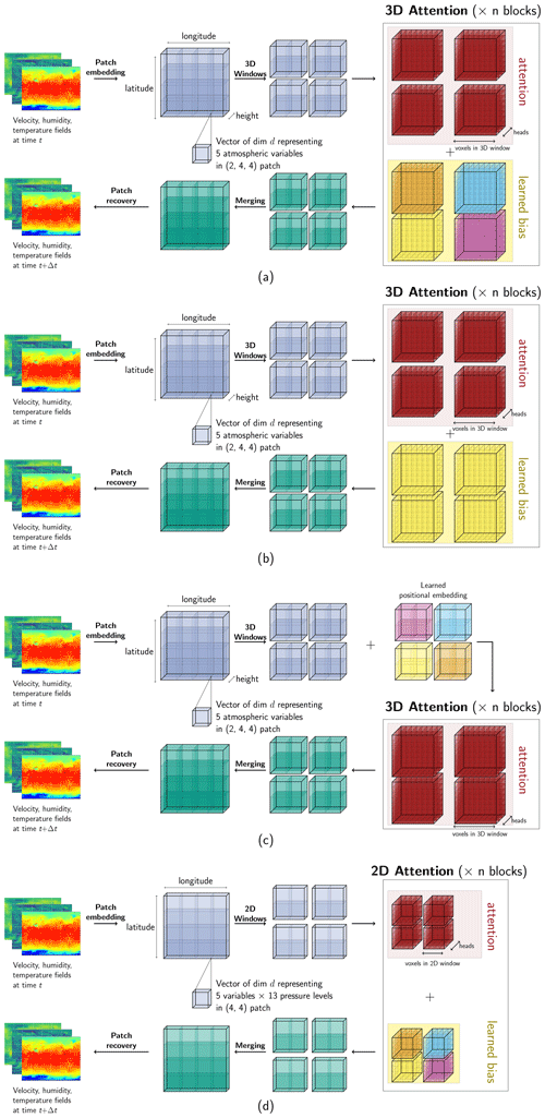
Figure 1 Architecture of the Pangu-Weather model and variations considered in the ablation study. The sliding-window mechanism (Swin) is not depicted in the figure for simplicity. The up- and downsampling layers are also excluded from the figure. (a) Pangu-Weather. (b) Relative bias. (c) Learned positional embedding. (d) 2D attention.

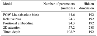
In the ablation study, five models were compared. These models and the number of parameters are shown in Table 1 and are described in more detail as follows.

Table 1 Overview of models included in the ablation study. All models are based on PGW-Lite.

In the PGW-Lite model, an absolute ESB term within the Transformer was implemented according to the description in Bi et al. (2023a). The formulation of self-attention in the PGW model is

$$\begin{array}{}\text{(1)}& \mathrm{attention}\left(\mathbf{Q},\mathbf{K},\mathbf{V}\right)=\mathrm{SoftMax}\left({\mathbf{QK}}^T/\sqrt{D}+{\mathit{B}}_{\mathrm{ESP}}\right)\mathbf{V}\end{array}$$

where Q, K, and V are the query, key, and value matrices and D is the feature dimensionality of Q. B_ESP was introduced by Bi et al. (2023a) to represent a bias term that varies as a function of latitude and height but is invariant to longitude. Bi et al. (2023a) reasoned that atmospheric fields are variable in the latitude and vertical dimensions but remain consistent in the longitude dimension. Even in the lite model, this term contains 20 million parameters, comprising 50 % of the overall terms in the model. In the relative bias model, the bias is invariant in all three spatial dimensions, reducing the model size to 24.3 million parameters. In the positional encoding model, the patches are given a learnable positional encoding term implemented similarly to in PGW-Lite in that the patches in the latitude and vertical dimensions learn a positional embedding with a hidden dimension of C=192 and the values stay the same along the longitude dimension. As this term is completely outside of the attention blocks, it requires far fewer parameters to implement. The three-depth model increases the depth of the network to three; i.e., two up- and downsampling layers were implemented. To keep the model size manageable, only four layers within the deepest block were implemented. As with the original model, the downsampling was implemented in the latitude and longitude dimensions by patches of (2, 2) and by increasing the hidden dimension 4-fold with a linear layer. In the 2D-Transformer model, the structure of PGW-Lite was retained, but the atmospheric variables of the different pressure levels were treated as different variables (channels). The attention mechanism in the Transformer block was only applied over values in the longitude and latitude dimensions. To compensate for the reduction in parameters associated with a 2D-Transformer model, the hidden dimension was increased from C=192 to C=288, increasing the dimension of the hidden layer to 48 per attention head as opposed to the original 32. Note that the latent space in the 2D Transformer now encodes 5 variables × 13 pressure levels instead of just 5 variables × 1 pressure level as in the 3D case.

2.6 Minibatch size and model training

A study directly comparing the PGW-Lite model, which features a 3D-attention mechanism, and the 2D-attention model was performed. Each of the two models was trained from scratch five times, varying the global batch size according to the following values: 16, 32, 64, 480, and 720. More experiments could not be conducted due to computational constraints. The details of the local and global minibatch size, as well as the average total GPU hours per epoch and wall time per epoch, are shown in Table 3. All models were initialized with the same random seed, so the orders of the training samples loaded from the data loader are identical.

2.7 Variable-specific weighted cosine loss scheduling

The loss function in PGW is defined as

$$\begin{array}{}\text{(2)}& {\displaystyle }\mathrm{loss}{\displaystyle }=\sum _i{w}_i\cdot L^{\mathrm{1}}\left(\mathrm{prediction},\mathrm{target}\right),\end{array}$$

where i is the variable, w is a weighting factor, L¹ is the L¹ loss function, prediction denotes the model outputs, and target denotes the ground-truth forecast data. The values of w_i are $\mathrm{3.00},\mathrm{0.6},\mathrm{1.5},\mathrm{0.77}$, and 0.54 for Z, Q, T, U, and V, and surface-variable weights are $\mathrm{1.5},\mathrm{0.77},\mathrm{0.66}$, and 3.00 for variables MSP, U, V, and T, as specified by Bi et al. (2023a).

After determining that the 2D-Transformer model appears to converge the fastest and require the fewest computational resources, we re-train the 2D-Transformer model from scratch for 300 epochs with a smooth loss function that weights the variables differently over the epochs. The loss function is designed so that within 100 epochs, the weights for each variable cycle through one cosine schedule (Fig. 2).

Given an individual variable i at epoch e, for a period of n_epochs (here, n_epoch=100), the formulation of the weighting factor is as follows: for the pressure variables Z, Q, T, U, and V, i=1, 3, 2, 0, and 0, respectively. For the surface variables MSP, U10, V10, and T2M, i=1, 0, 0, and 2, respectively.

$$\begin{array}{}\text{(3)}& {\displaystyle }w(i,e)=\cos \left({\displaystyle \frac{\mathrm{2}\mathit{\pi }}{n_{\mathrm{epoch}}}}\left(e-{\displaystyle \frac{i}{\mathrm{2}}}\right)\right)+\mathrm{1.1}\end{array}$$

At each epoch, the pressure variables are normalized to sum up to the original weights of $\mathrm{3.00}+\mathrm{0.60}+\mathrm{1.50}+\mathrm{0.77}+\mathrm{0.54}$.

$$\begin{array}{}\text{(4)}& {\displaystyle }W(i,e)=w(i,e)\cdot {\displaystyle \frac{\mathrm{3.00}+\mathrm{0.60}+\mathrm{1.50}+\mathrm{0.77}+\mathrm{0.54}}{{\sum }_{i}w(i,e)}}\end{array}$$

A similar procedure is applied to the surface variables, where the numerator is replaced with $\mathrm{1.5}+\mathrm{0.77}+\mathrm{0.66}+\mathrm{3.0}$. The ordering of the weights was designed such that the weights of the velocity and temperature variables (U, U10; V, V10; T, T2M) would peak at similar epochs.

The validation loss is always calculated with the original weights to maintain consistency. Note that the two schedules for the pressure level and surface variables are complementary: the weights for velocity fields and temperature at both levels are in phase.

Figure 2 The weights for variable-specific cosine loss scheduling. The period is 100 epochs. The U- and V-velocity fields for both the pressure-level variables and the surface variables are superimposed on one another, since they always receive the same values. The weights are normalized to sum up to the sum of the original weights presented in Bi et al. (2023a). (a) Pressure-level variables. (b) Surface variables.

3 Results

3.1 Validation

A representative output of the model for a 24 h forecast as well as the absolute error is visualized in Fig. 3.

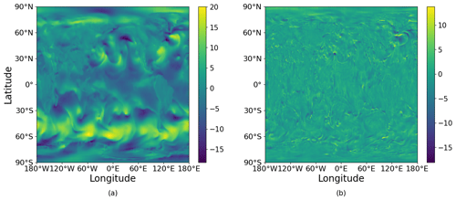
Figure 3 Representative sample of the U-velocity field at a pressure level of 1000 hPa for a 24 h forecast. The forecast was initialized on 26 January 2020 at 00:00 UTC. (a) U-velocity field. The color bar represents the U velocity in units of m s⁻¹. (b) Absolute error. The color bar represents the absolute error between the prediction and the ground truth.

Figure 4 shows the RMSE with an increasing lead time of two surface variables, U velocity at 10 m and the temperature at 2 m, as well as temperature at a pressure level of 850 hPa, tested over the years 2020 and 2021. We observe that our PGW model performs better than IFS for three variables (U10, T2M, T850) over the 5 d forecast, but it performs worse for the Z500 variable. There is still a notable difference between the performance of our model and the published PGW model. We attribute this to training the model on only a 6 h subsample of the total data trained by the original authors, as well as to slight differences in the training procedure such as batch size. While our model cannot compete with the published PGW model by Bi et al. (2023a), this result gives us enough confidence that complex weather patterns can be learned with our model for us to proceed with the ablation study.

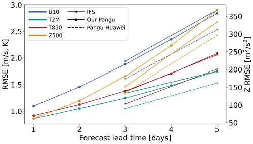
Figure 4 RMSE as a function of the forecast lead time of key prognostic variables (T2M, U10, T850) in our model compared to IFS and Pangu-Weather on testing data from 2020–2021. RMSE values of temperature and velocity are on the left y axis, and the RMSE values of geopotential are on the right y axis. Pangu-Huawei refers to the reference model.

3.2 Ablation study

The training and validation losses of the different models are shown in Fig. 5. All of the validation losses closely parallel the training losses, indicating that none of the models are overfitted. Despite drastic variations in the model architecture and in the size of the networks, all models exhibit similar loss curves. Furthermore, they reach similar final loss values upon model convergence.

As the loss function for the model is the L¹ loss, we also wish to verify that meteorologically relevant metrics such as the RMSE and the anomaly correlation coefficient improve for specific variables as the L¹ loss goes down. Figure 5 shows the weighted RMSE values of the U velocity at 10 m. Though all models learn with a similar structure, we note that the 2D Transformer is able to reach some of the lowest RMSE values at a given epoch, i.e., the compute budget.

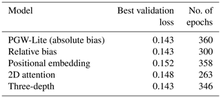
The best validation loss as well as the epoch in which that is reached is shown in Table 2. All models reach a similar validation loss, with the value for the positional embedding being the worst at 0.152 and the PGW-Lite, relative bias, and three-depth models tying for the best at 0.143. However, it is important to note that the 2D model converged 40–100 epochs earlier than the other models, reducing computation by 11 %–28 %. Furthermore, Sect. 3.3 shows that reducing the batch size allows the 2D Transformer to converge to lower values of the loss function within fewer epochs compared to PGW-Lite.

Figure 5 Training curves of ablation study for the PGW-Lite, three-depth, relative bias, positional embedding, and 2D-attention models. (a) Training and validation loss values as a function of the epochs. (b) RMSE for the 10 m U velocity as a function of the epochs, as evaluated for the validation samples.

Table 2 Best validation loss and total epochs for the different models.

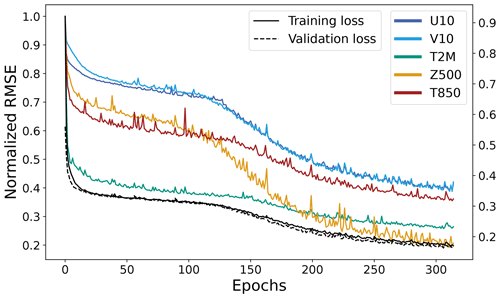
Figure 6 shows the development of the RMSE for different variables as the model continues to learn for the PGW-Lite model trained on a global minibatch size of 720. For the first 230 epochs, the learning rate is kept constant at $\mathrm{5}\times {\mathrm{10}}^{-\mathrm{4}}$. As paralleled in the validation loss plots in Fig. 5, the model learns relatively slowly for the first 100 epochs except for during the initial drop. After that, particularly in the velocity and geopotential fields, the model is able to learn more quickly before reaching a second plateau. Though it is not shown here, we observe similar patterns for all ablated models.

Figure 6 RMSE as a function of epochs for different prognostic variables for PGW-Lite, as evaluated on the validation dataset. All values are normalized by their maximum RMSE value.

3.3 Minibatch size effects

Figure 7 shows the validation loss of two models, PGW-Lite and 2D attention, with a global minibatch size of 16, 32, 64, 480, and 720. Both models train nearly identically for a minibatch size of 16 but diverge for all other minibatch sizes. For the 2D-Transformer model, similar final loss values were reached for minibatch sizes of 16, 64, and 480. The 2D-Transformer model appears to have instabilities in the beginning of training for a batch size of 32, leading it to converge at a worse final loss value. For the 2D model, it appears that using a small global minibatch size reduces the time to convergence and improves the final model performance. In contrast, the PGW-Lite model converges at sub-optimal loss values for minibatch sizes of 16, 32, and 480. In these cases, the models were allowed to train until the learning rate dropped to $\mathrm{3}\times {\mathrm{10}}^{-\mathrm{5}}$. The irregularity of this behavior can be attributed to the model's sensitivity to the initial random seed.

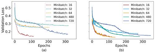
Figure 7 Validation loss as a function of epochs for global minibatch sizes of 16, 32, 64, 480, and 720 of (a) the 2D attention model and (b) PGW-Lite.

Table 3 Compute requirements for PGW-Lite and the 2D-attention model (2D Transformer) based on minibatch size.

The global minibatch size greatly affects the speed of convergence: by training with a smaller global minibatch size, we reach lower values of the loss function much more quickly; this also comes with a reduction in overall compute power but at the cost of longer wall times.

3.4 Variable-specific weighted cosine loss scheduling

Figure 8 shows the RMSE of the variables U10, V10, T850, and T2M over the course of the cosine loss scheduling. The final L¹ loss value reached was 0.131, lower than all other models trained in this paper. The large fluctuations in the training loss reflect the cosine scheduling of the different variables. The RMSEs of the different key variables are shown alongside the training and validation loss in Fig. 8.

Figure 8 Error metrics for variable-specific weighted cosine loss scheduling applied to the 2D-attention model. The 2D-attention model with PyTorch's ReduceLROnPlateau scheduler was maintained as the reference model and compared to the variable-specific weighted cosine loss scheduling model. (a) RMSE values of the 10 m U and V velocities, as evaluated on the validation dataset, as a function of the epochs. (b) Training and validation losses for the two models.

Despite the large fluctuations in the training loss, the validation loss continues to decrease. There are some fluctuations in the RMSE variables, reflecting the effects of the weight scheduling: between epochs 125 and 175, the weights for the velocity fields are small. In this period, we notice that the validation RMSEs for the velocity variables increase slightly as the temperature, weighted highly, decreases.

4 Discussion

4.1 Ablation study

The major finding of this ablation study is that neither of the two novel ideas introduced by PGW is crucial to its success. This underscores the idea that the success of PGW is due to the Transformer backbone and Swin mechanism rather than to the particular bias term introduced or the 3D-Transformer architecture. This is noteworthy because these two architectural components are particularly expensive with respect to training time and memory requirement. In fact, the PGW-Lite model does not perform better than the other ablated smaller models. The three-depth model, the largest and deepest configuration, was expected to perform significantly better. This is because, in its deepest layers, the individual windows in Swin are designed to apply attention across greater ranges, enabling the model to capture and learn far-reaching weather patterns. Surprisingly, the model appears to be difficult to train and to have convergence issues; the final performance of the three-depth model was not better than that of PGW-Lite. The results of this study show that the massive ESB term can be replaced by simple learned positional embedding, reducing the size of the term that learns the Earth-specific locality by 20.4 million parameters, even in the case of PGW-Lite; in the case of the full PGW model, this term contains 40.4 million of the total 64.2 million parameters.

Table 2 and Fig. 5 show that the 2D-attention mechanism is a suitable replacement for the 3D Transformer. They show that the 2D Transformer learns the representation faster than any of the 3D models, reaching a comparable validation loss and RMSE value in fewer epochs. Intuitively, we expect that the 3D Transformer introduced in Bi et al. (2023a) should perform better than the 2D Transformer. However, evaluating these results shows that the 2D Transformer is sufficient. This can be explained by the change in architecture. After patch embedding, a representation of all variables in each is learned and stored in a latent vector of dimension C. With a 3D-Transformer architecture, each latent vector contains the information of the five pressure variables (Z, Q, T, U, V) and attention is performed between neighboring patches in all dimensions. In a 2D-Transformer architecture, the latent vector contains the five pressure variables at all pressure levels and attention is only performed over the neighboring patches in the latitude and longitude dimensions. It is possible that mixing the information across all spatial layers is more efficient, as it allows the model to learn the relationship between more than two pressure levels at a time. This has many benefits – by using the 2D-attention model, the individual attention blocks require much less memory. Specifically, the attention mechanism requires an O(n²) memory requirement with respect to the size of the sequence (Vaswani et al., 2017). Reducing the attention blocks to perform attention over patches from (2, 6, 12) to (1, 6, 12) in the 2D Transformer has allowed us to double the local minibatch size per GPU, reducing the total computational requirements.

Due to the infinitely large hyperparameter space and apparent sensitivity of the model to these parameters, it is unclear whether the presence of the 3D Transformer or ESB is truly detrimental to the convergence and success of the model. It is entirely possible that, given the correct hyperparameter configuration, the original PGW model could greatly outperform these cheaper, ablated models. However, due to the cost, energy requirements, and associated CO₂ emissions of the compute requirements of the original model, we argue that it is important to develop easily trainable and robust models; we strive for a model with little hyperparameter tuning, reducing the compute requirements of training. Figures 5 and 7 show that all models follow two phases of training: after a certain point, the model learns a suitable embedded representation and can proceed to learn more quickly. In this work, we explore different mechanisms to reduce the number of epochs it takes these models to reach this trigger point; this reduces the computational burden and makes these data-driven models accessible to researchers with smaller compute budgets.

4.2 Batch size

The difficulty and the unpredictability of training Transformers are shown in Fig. 7, where the PGW-Lite and 2D-attention models were trained for different global minibatch sizes of 16, 32, 64, 480, and 720. All models were initialized with the same random seed. With the exception of minibatch size 16, the 2D-attention model was trained within fewer epochs than the equivalent PGW-Lite model. While the 2D-attention minibatch 32 model also showed instability and difficulty in training, PGW-Lite with minibatches of 32, 64, and 480 failed to converge and leave the phase 1 stage of training. Despite the learning rate dropping to small values of $\mathrm{3}\times {\mathrm{10}}^{-\mathrm{5}}$, the models did not improve and training was stopped. The results indicate that the higher model complexity in PGW also increases the difficulty in convergence. The trends in this experiment are non-monotonous (e.g., global minibatch sizes of 16 and 64 converged to low loss values in the 2D-attention model, but a minibatch size of 32 performed worse) and difficult to explain – we hypothesize that training several models with different random seeds would help in finding at least one model that converges to a low loss value. Given that many researchers face limited compute budgets, this underscores the benefit of having a model that is robust to training and hyperparameters.

Table 3 shows that the 2D models consistently require fewer total GPU hours and less wall time to train compared to the PGW-Lite models, despite having more model parameters. This highlights the computational cost of the attention mechanism, as the PGW-Lite model performs attention across windows that are 2 times larger than the 2D-attention model. For both models, doubling the GPUs results in a speedup of between 80 %–95 %, revealing the increased synchronization time required with more parallelization. When comparing the run times for global minibatch sizes of 480 and 720, the 2D-attention model is able to fit 2 times the number of samples per GPU. This comes at the expense of wall time, where we see the 2D models requiring between 1.5 and 1.7 times more wall time to complete a given epoch but having similar overall computational demands.

The relationship between average total GPU hours per epoch and batch size exhibited by the 2D-attention model shows that using smaller minibatch sizes will reduce the computational time per epoch, at the cost of wall time. Combined with the speedup in convergence behavior – i.e., a smaller global batch size leads to fewer overall epochs required – the results indicate the benefits of using both smaller local and smaller global batch sizes when training weather forecasting models. Our limited results emphasize the need for more systematic studies on the relationship between local and global batch sizes, wall time, and convergence.

4.3 Variable-specific weighted cosine loss scheduling

This study highlights the sensitivity of Transformer-based medium-range weather forecasting models to hyperparameters such as batch size and learning rate. With this in mind, we wanted to develop some explainable heuristics that could be applied to the training scheduling. The advantages of training an autoregressive weather forecasting model are that the input and output fields are the same and that the fields describe physical dynamics. We look at the RMSE over epochs in Fig. 6 to understand how the model learns. We notice a few trends: as expected, the U- and V-velocity fields learn at the same rates. The temperature fields level off more quickly, whereas the geopotential field continues to improve as training goes on, even when the loss function appears to have stagnated.

The design behind the variable-specific weighted cosine scheduling is because it was observed that the velocity fields, compared to fields such as geopotential or temperature, take longer to learn. This is attributed to the sharp and localized gradients that occur in these fields, making them harder to learn and generalize. However, in atmospheric models, resolving the velocity fields is crucial, since wind vectors, acting as pressure gradients, can drive certain atmospheric processes such as advection terms in atmospheric variables. As such, we decided to schedule the weights in such a way that the velocity fields are encouraged to improve quickly in the beginning, at the cost of learning other fields such as the temperature in the beginning.

Figure 8 shows that even as the training loss fluctuates due to a variable-specific weighted scheduling, the validation RMSE values of different variables will generally continue improving, with only minor fluctuations. Particularly in the beginning of training, the implementation of the variable-specific weighted cosine loss scheduling allows the model to converge with approximately 30 % fewer epochs, with all other hyperparameters and training regimens kept constant.

5 Conclusions

This work presents an ablation study of PGW to determine the important architectural components that lead to its success. It finds that the ESB can be replaced with a simple relative bias, reducing the overall number of model parameters by 46 %. We also show that replacing the 3D Transformer with a 2D Transformer, even though it has 30 % more parameters, allows for the model to fit more samples on a single GPU – in our case, 2 times that of the former. Furthermore, the 2D models consistently train faster than or just as fast as the three-dimensional models and reach better L¹ and RMSE values upon convergence. An initial study on the batch size effects of these models shows that the 2D Transformer is much more robust to training than PGW-Lite, which often failed to converge. We also show that training either model with a global minibatch size of 16 and a local batch size of 1 can allow the model to converge within 28 % of the total epochs, compared to a minibatch size of 720, while maintaining similar total GPU hours per epoch and increasing the wall time sub-linearly. This points to further work in understanding the relationship between local and global batch sizes, total GPU hours required, and wall time. We also show that implementing a simple weighted loss function schedule over time can push the model to converge with nearly 30 % fewer epochs, effectively reducing the computational cost to reach a given performance at no change to the model architecture or training schedule.