GNNWR: an open-source package of spatiotemporal intelligent regression methods for modeling spatial and temporal nonstationarity

Spatiotemporal regression is a crucial method in geography for discerning spatiotemporal nonstationarity in geographical relationships and has found widespread application across diverse research domains. This study implements two innovative spatiotemporal intelligent regression models, i.e., Geographically Neural Network Weighted Regression (GNNWR) and Geographically and Temporally Neural Network Weighted Regression (GTNNWR), which use neural networks to estimate spatiotemporal nonstationarity. Due to the higher accuracy and generalization ability, these models have been widely used in various fields of scientific research. To facilitate the application of GNNWR and GTNNWR in addressing spatiotemporal nonstationary processes, the Python-based package GNNWR has been developed. This article details the implementation of these models and introduces the GNNWR package, enabling users to efficiently apply these cutting-edge techniques. Validation of the package is conducted through two case studies. The first case involves the verification of GNNWR using air quality data from China, while the second employs offshore dissolved silicate concentration data from Zhejiang Province to validate GTNNWR. The results of the case studies underscore the effectiveness of the GNNWR package, yielding outcomes of notable accuracy. This contribution anticipates a significant role for the developed package in supporting future research that will leverage big data and spatiotemporal regression techniques.

1 Introduction

Spatiotemporal nonstationarity, denoting variations in geographical elements or structures across different temporal and spatial contexts, constitutes an intrinsic attribute of nearly all kinds of geographical processes and phenomena. Geographically weighted regression (GWR), a classic methodology for delineating spatial nonstationarity in geographical relationships, facilitates variations of parameter coefficients within a regression equation according to spatial locations (Brunsdon et al., 1996). As a foundational algorithm within the domain of spatiotemporal regression analysis, GWR has been widely used across diverse research domains, including environmental studies (Yang et al., 2019; Shen et al., 2023), urban studies (Sisman and Aydinoglu, 2022; He et al., 2023), and the social sciences (Stein et al., 2015; Lewandowska-Gwarda, 2018; Ahadnejad Reveshty et al., 2023).

On the basis of GWR, various methods have been proposed that focus on optimizing a model's ability to solve spatiotemporal nonstationary relationships. The improvements mainly include the following aspects: the selection of spatiotemporal distance metrics (Fotheringham et al., 2015; Lu et al., 2014), the choice of weight kernel functions (Fotheringham et al., 2017), and the optimization of statistical diagnostic methods (Brunsdon et al., 1999; Leung et al., 2000). Notably, multiscale geographically weighted regression (MGWR) extends the weight kernel function to varying bandwidths for each independent variable and further enhances the model's capacity to fit spatial nonstationarity (Fotheringham et al., 2017). To deploy a MGWR model, researchers developed a Python-based software package, mgwr, that focuses on multiscale estimation and efficient computation of spatial nonstationarity (Oshan et al., 2019). It supplements R-language-based open-source tools, e.g., spgwr (Bivand and Yu, 2023), gwrr (Wheeler, 2022), and GWmodel (Lu et al., 2024), improving the overall accessibility of the GWR and MGWR methods.

Owing to the intricate linear interplay between spatial distance and nonstationary weights inherent in geographical processes, precise computation of the weight matrix through simple kernel functions faces notable challenges. In response to this, diverse methodologies within the domain of geospatial artificial intelligence (GeoAI) have been proposed to effectively capture nonlinear spatial relationships between pertinent factors (Georganos and Kalogirou, 2022; Hagenauer and Helbich, 2022). The majority of existing GeoAI approaches utilize neural networks in an opaque manner to establish spatial relationships, leading to constrained spatial interpretability of the estimated relationships. To address this, researchers have integrated a spatiotemporal weighted framework with neural networks, leading to the formulation of spatiotemporal intelligent regression models. Notably, the Geographically Neural Network Weighted Regression (GNNWR) model has been introduced, which employs neural networks to learn the nonlinear relationship between spatial distance and nonstationary weights (Du et al., 2020a). Taking inspiration from GWR, GNNWR employs a spatially weighted neural network (SWNN) to accurately derive the spatial weight matrix. Subsequently, this SWNN is combined with an ordinary linear regression (OLR) model to estimate spatial nonstationarity.

In addition to space, time is another fundamental dimension associated with geographical processes. In recent years, numerous studies have focused on incorporating temporal effects into GWR models to account for both temporal and spatial nonstationarity (Huang et al., 2010; Fotheringham et al., 2015). Recognizing that time and space exhibit distinct scale effects, Huang et al. (2010) proposed a straightforward approach to combine spatial and temporal distances into a unified space–time distance, leading to the development of the Geographically and Temporally Weighted Regression (GTWR) model. The GTWR model, along with its extended methodologies, has been effectively applied across various domains, producing remarkable results and offering satisfactory interpretability (Ma et al., 2018; He and Huang, 2018; Guo et al., 2021; Wang et al., 2022).

However, the form of space–time distance usually requires a priori assumptions and should be assumed to be relatively simple (e.g., a linear weighted function) so as to eliminate the estimation problem in the terminal model. Considering that neural networks have the potential to capture complex nonlinear effects in space and time, Wu et al. (2021) proposed a spatiotemporal proximity neural network (STPNN) to accurately generate space–time distance and extended GNNWR with the STPNN to incorporate temporal effects into spatial nonstationarity. Accordingly, a spatiotemporal intelligent regression model, Geographically and Temporally Neural Network Weighted Regression (GTNNWR), was developed to estimate spatiotemporal nonstationary relationships.

In recent years, GNNWR and GTNNWR have been widely applied in various fields and have achieved excellent fitting capabilities and geographical interpretability, such as for atmospheric pollution (Chen et al., 2021; Ni et al., 2022; Liu et al., 2023), environmental modeling (Wu et al., 2019; Du et al., 2021; Wu et al., 2022; Qi et al., 2023), and urban geography (Wang et al., 2022; Yang et al., 2022; Liang et al., 2023). However, the accessible versions for the source code of GNNWR (Du, 2019) and GTNNWR (Wu, 2020) are implemented with TensorFlow 1.x, which is too old to run in the latest hardware environment. The codes are not highly encapsulated, which makes it harder for researchers to use and develop the model. Therefore, there is a need to develop a set of model implementations with a newer architecture, simpler usage, and clearer code structure to facilitate the utilization of these spatiotemporal intelligent regression models by researchers in different fields and to solicit feedback for refinement and enhancement of these models.

This research has developed an open-source Python package, denoted the GNNWR package, to furnish a suite of spatiotemporal intelligent regression models encompassing the GNNWR and GTNNWR variants, thereby serving as a resource for researchers seeking to address challenges within their respective fields. The GNNWR package offers a comprehensive workflow analysis capability, enabling users to create datasets, instantiate models, conduct training, generate output results, and perform model predictions and visualizations. The GNNWR package uses PyTorch as a deep-learning framework (Paszke et al., 2019), and its dynamic computational graph makes model construction and debugging more intuitive. This package provides extended models and great flexibility, allowing advanced users to design custom models based on existing models using the PyTorch framework.

The remainder of this article is constructed as follows. In Sect. 2, we provide a review of the GNNWR and GTNNWR models that the package has implemented. In Sect. 3, we describe the package architecture and offer a usage example for the package. Finally, in Sect. 4, we conclude with a summary of our outcomes and suggest potential avenues for future development.

2 Model review

This section offers a concise overview of the GNNWR family of models, which are accommodated by the GNNWR package. Detailed descriptions and performance analysis can be found in the original articles (Du et al., 2020a; Wu et al., 2021).

2.1 OLR and GWR

For a regression relation to p independent variables and n observations, the regression formula of the classic OLR model is expressed as

$$\begin{array}{}\text{(1)}& y_i={\mathit{\beta }}_{\mathrm{0}}^{\mathrm{OLR}}+\sum _{k=\mathrm{1}}^p{\mathit{\beta }}_k^{\mathrm{OLR}}{x}_{ik}+{\mathit{\epsilon }}_i\text{ for }i=\mathrm{1},\mathrm{2},\mathrm{\dots },n,\end{array}$$

where y_i and x_ik are the dependent variable and kth independent variable at observation i, ${\mathit{\beta }}_k^{\mathrm{OLR}}$ is the regressive coefficient for the kth independent variable, ${\mathit{\beta }}_{\mathrm{0}}^{\mathrm{OLR}}$ is the intercept term, and ε_i is the error term.

Considering the spatial nonstationarity, the GWR model extends the OLR approach to enable spatially localized estimates by allowing local variations in rates of change. Thus, the regression can be represented as

$$\begin{array}{}\text{(2)}& y_i={\mathit{\beta }}_{\mathrm{0}}(u_i,v_i)+\sum _{k=\mathrm{1}}^p{\mathit{\beta }}_k(u_i,v_i)x_{ik}+{\mathit{ϵ}}_i\text{ for }i=\mathrm{1},\mathrm{2},\mathrm{\dots },n,\end{array}$$

where β₀(u_i,v_i) and β_k(u_i,v_i) are the localized regression coefficients for the constant term and the kth independent variable at location (u_i,v_i). Their estimation can be calculated with a weighted least-squares method:

$$\begin{array}{}\text{(3)}& \widehat{\mathit{\beta }}(u_i,v_i)=\left({\mathbf{X}}^{\top }\mathbf{W}\right(u_i,v_i\left)\mathbf{X}{)}^{-\mathrm{1}}{\mathbf{X}}^{\top }\mathbf{W}\right(u_i,v_i)\mathbf{y},\end{array}$$

where W(u_i,v_i) is the spatial weighting diagonal matrix at fit point i, and y and X are the dependent and independent variables for all the observations. A distance-decaying kernel function (e.g., a Gaussian kernel) is then employed to calculate the spatial weights from the fit point to its neighboring observations within the bandwidth b:

$$\begin{array}{}\text{(4)}& w_{ij}=\exp [-(d_{ij}/b{)}^{\mathrm{2}}],\end{array}$$

where d_ij is the distance between fit point i and its neighbor j.

2.2 GNNWR

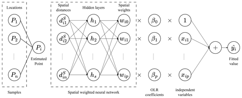
Since a predefined kernel function might not accurately estimate complex, heterogenous geographical processes, the GNNWR model introduces an SWNN to represent the nonstationary weight matrix (Fig. 1).

The spatial weight estimation for point i is calculated as follows:

$$\begin{array}{}\text{(5)}& \mathbf{W}(u_i,v_i)=\mathrm{SWNN}\left(\right[d_{i\mathrm{1}}^{\mathrm{S}},d_{i\mathrm{2}}^{\mathrm{S}},\mathrm{\dots },d_{\mathrm{in}}^{\mathrm{S}}{]}^{\top }),\end{array}$$

where $[d_{i\mathrm{1}}^{\mathrm{S}},d_{i\mathrm{2}}^{\mathrm{S}},\mathrm{\dots },d_{in}^{\mathrm{S}}]$ are the distances from location i to the other training samples, and the weighting matrix W(u_i,v_i) is a diagonal matrix whose diagnostic elements are the nonstationary weights $w_{\mathrm{0}}(u_i,v_i),w_{\mathrm{1}}(u_i,v_i),\mathrm{\dots },w_p(u_i,v_i)$ for the regression.

Accordingly, the GNNWR model describes spatial nonstationarity through fluctuating changes in the coefficients of OLR at different locations (Du et al., 2020a). Thereby, the spatial nonstationarity can be represented as

$$\begin{array}{}\text{(6)}& \begin{array}{rl}& y_i=w_{\mathrm{0}}(u_i,v_i){\mathit{\beta }}_{\mathrm{0}}^{\mathrm{OLR}}+\sum _{k=\mathrm{1}}^p{w}_k(u_i,v_i){\mathit{\beta }}_k^{\mathrm{OLR}}{x}_{ik}+{\mathit{ϵ}}_i\\ & \text{for }i=\mathrm{1},\mathrm{2},\mathrm{\dots },n.\end{array}\end{array}$$

Then, the estimates of dependent variables in GNNWR can be calculated as

$$\begin{array}{}\text{(7)}& \begin{array}{rl}\widehat{\mathit{y}}& =\left[\begin{array}{c}{\widehat{y}}_{\mathrm{1}}\\ {\widehat{y}}_{\mathrm{2}}\\ \mathrm{⋮}\\ {\widehat{y}}_n\end{array}\right]=\left[\begin{array}{c}{\mathit{x}}_{\mathrm{1}}^{\top }\mathbf{W}(u_{\mathrm{1}},v_{\mathrm{1}})({\mathbf{X}}^{\top }\mathbf{X}{)}^{-\mathrm{1}}{\mathbf{X}}^{\top }\\ {\mathit{x}}_{\mathrm{2}}^{\top }\mathbf{W}(u_{\mathrm{2}},v_{\mathrm{2}})({\mathbf{X}}^{\top }\mathbf{X}{)}^{-\mathrm{1}}{\mathbf{X}}^{\top }\\ \mathrm{⋮}\\ {\mathit{x}}_n^{\top }\mathbf{W}(u_n,v_n)({\mathbf{X}}^{\top }\mathbf{X}{)}^{-\mathrm{1}}{\mathbf{X}}^{\top }\end{array}\right],\\ \mathit{y}& =\left[\begin{array}{c}{{\mathit{x}}_{\mathbf{1}}}^{\top }\mathrm{SWNN}\left(\right[d_{i\mathrm{1}}^{\mathrm{S}},d_{i\mathrm{2}}^{\mathrm{S}},\mathrm{\dots },d_{in}^{\mathrm{S}}{]}^{\top }\left)\right({\mathbf{X}}^{\top }\mathbf{X}{)}^{-\mathrm{1}}{\mathbf{X}}^{\top }\\ {{\mathit{x}}_{\mathbf{2}}}^{\top }\mathrm{SWNN}\left(\right[d_{i\mathrm{1}}^{\mathrm{S}},d_{i\mathrm{2}}^{\mathrm{S}},\mathrm{\dots },d_{in}^{\mathrm{S}}{]}^{\top }\left)\right({\mathbf{X}}^{\top }\mathbf{X}{)}^{-\mathrm{1}}{\mathbf{X}}^{\top }\\ \mathrm{⋮}\\ {{\mathit{x}}_{\mathit{n}}}^{\top }\mathrm{SWNN}\left(\right[d_{i\mathrm{1}}^{\mathrm{S}},d_{i\mathrm{2}}^{\mathrm{S}},\mathrm{\dots },d_{in}^{\mathrm{S}}{]}^{\top }\left)\right({\mathbf{X}}^{\top }\mathbf{X}{)}^{-\mathrm{1}}{\mathbf{X}}^{\top }\end{array}\right]\mathit{y}=\mathbf{Sy},\end{array}\end{array}$$

where S is the hat matrix of the GNNWR model.

Figure 1 The framework of the GNNWR model.

2.3 GTNNWR

Alongside space, time constitutes a fundamental dimension in the study of geographic phenomena. The GTNNWR model extends the spatial form of the nonstationary relationship in Eq. (6) to the following spatiotemporal form:

$$\begin{array}{}\text{(8)}& \begin{array}{rl}{y}_i& ={\mathit{\beta }}_{\mathrm{0}}(u_i,v_i,t_i)+\sum _{k=\mathrm{1}}^p{\mathit{\beta }}_k(u_i,v_i,t_i)x_{ik}+{\mathit{\epsilon }}_i\\ & =w_{\mathrm{0}}(u_i,v_i,t_i){\mathit{\beta }}_{\mathrm{0}}^{\mathrm{OLR}}+\sum _{k=\mathrm{1}}^p{w}_k(u_i,v_i,t_i){\mathit{\beta }}_k^{\mathrm{OLR}}{x}_{ik}\\ & +{\mathit{\epsilon }}_i,\text{ for }i=\mathrm{1},\mathrm{2},\mathrm{\dots },n,\end{array}\end{array}$$

where $w_k(u_i,v_i,t_i)$ represents the spatiotemporal nonstationary weight of ${\mathit{\beta }}_k^{\mathrm{OLR}}$, which is determined by its spatiotemporal location $(u_i,v_i,t_i)$ and is influenced by other samples.

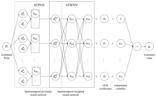
Similar to the SWNN of GNNWR, the GTNNWR model designed a spatiotemporal weighted neural network (STWNN) to calculate the spatiotemporal weights as follows:

$$\begin{array}{}\text{(9)}& \mathbf{W}(u_i,v_i,t_i)=\text{STWNN}\left({\left[d_{i\mathrm{1}}^{\mathrm{ST}},d_{i\mathrm{2}}^{\mathrm{ST}},\mathrm{\dots },d_{in}^{\mathrm{ST}}\right]}^{\top }\right),\end{array}$$

where $\left[d_{i\mathrm{1}}^{\mathrm{ST}},d_{i\mathrm{2}}^{\mathrm{ST}},\mathrm{\dots },d_{in}^{\mathrm{ST}}\right]$ are the spatiotemporal distances from point i to other training samples. This expression indicates that the spatiotemporal nonstationary weight is determined by the spatiotemporal distance. To quantify the spatiotemporal distance, Huang et al. (2010) defined the distance as having the following form:

$$\begin{array}{}\text{(10)}& d_{ij}^{\mathrm{ST}}=d_{ij}^{\mathrm{S}}\otimes d_{ij}^{\mathrm{T}},\end{array}$$

where ⊗ represents a fusion operator which integrates temporal ($d_{ij}^{\mathrm{T}}$) and spatial ($d_{ij}^{\mathrm{S}}$) distances into a spatiotemporal distance $d_{ij}^{\mathrm{ST}}$.

To fully capture the nonlinear effects in the spatiotemporal dimension, Wu et al. (2021) proposed a STPNN as the fusion operator ⊗. Therefore, the spatiotemporal weight matrix for any given point across time and space can be derived by merging the STPNN with the STWNN (Fig. 2):

$$\begin{array}{}\text{(11)}& \begin{array}{rl}\mathbf{W}(u_i,v_i,t_i)& =\text{STWNN}\left({\left[d_{i\mathrm{1}}^{\mathrm{ST}},d_{i\mathrm{2}}^{\mathrm{ST}},\mathrm{\dots },d_{in}^{\mathrm{ST}}\right]}^T\right)\\ & =\text{STWNN}\left(\left[\text{STPNN}\left(d_{i\mathrm{1}}^{\mathrm{S}},d_{i\mathrm{1}}^{\mathrm{T}}\right)\right.\right.\\ & \left.{\left.\mathrm{\dots },\text{STPNN}\left(d_{in}^{\mathrm{S}},d_{in}^{\mathrm{T}}\right)\right]}^T\right).\end{array}\end{array}$$

The spatiotemporal weights are then integrated with global OLR estimates, generating continuous coefficients varying in space and time, and the regression relationship of GTNNWR can be expressed as

$$\begin{array}{}\text{(12)}& \begin{array}{rl}{y}_i& =w_{\mathrm{0}}(u_i,v_i,t_i){\mathit{\beta }}_{\mathrm{0}}^{\mathrm{OLR}}\\ & +\sum _{k=\mathrm{1}}^p{w}_k(u_i,v_i,t_i){\mathit{\beta }}_k^{\mathrm{OLR}}{x}_{ik}+{\mathit{ϵ}}_i\text{ for }i=\mathrm{1},\mathrm{2},\mathrm{\dots },n,\end{array}\end{array}$$

where $w_k(u_i,v_i,t_i)$ are the diagonal elements of the spatiotemporal weight matrix $\mathbf{W}(u_i,v_i,t_i)$.

The estimated dependent variables $\widehat{y}$ can be calculated as

$$\begin{array}{}\text{(13)}& {\displaystyle }\widehat{\mathit{y}}=\left[\begin{array}{c}{\widehat{y}}_{\mathrm{1}}\\ {\widehat{y}}_{\mathrm{2}}\\ \mathrm{⋮}\\ {\widehat{y}}_n\end{array}\right]=\left[\begin{array}{c}{\mathit{x}}_{\mathrm{1}}^{\top }\mathbf{W}(u_{\mathrm{1}},v_{\mathrm{1}},t_{\mathrm{1}})({\mathbf{X}}^{\top }\mathbf{X}{)}^{-\mathrm{1}}{\mathbf{X}}^{\top }\\ {\mathit{x}}_{\mathrm{2}}^{\top }\mathbf{W}(u_{\mathrm{2}},v_{\mathrm{2}},t_{\mathrm{2}})({\mathbf{X}}^{\top }\mathbf{X}{)}^{-\mathrm{1}}{\mathbf{X}}^{\top }\\ \mathrm{⋮}\\ {\mathit{x}}_n^{\top }\mathbf{W}(u_n,v_n,t_n)({\mathbf{X}}^{\top }\mathbf{X}{)}^{-\mathrm{1}}{\mathbf{X}}^{\top }\end{array}\right]\mathit{y}=\mathbf{Sy},\end{array}$$

where S is the hat matrix of the GTNNWR model.

Figure 2 The framework of the GTNNWR model. $d_{ij}^{\mathrm{S}}$ and $d_{ij}^{\mathrm{T}}$ represent the spatial distance and temporal distance between the estimated points P_i and P_j, respectively. The spatiotemporal proximity $d_{ij}^{\mathrm{ST}}$ is obtained by integrating $d_{ij}^{\mathrm{S}}$ and $d_{ij}^{\mathrm{T}}$ through the STPNN.

3 Package descriptions

In this section, we present a comprehensive overview of the gnnwr package (version 0.1.11) and the range of models it supports. We begin by introducing the fundamental architecture of the software package, delving into its essential components and functionalities. Following this, we outline the analysis process employed in utilizing the package, showcasing its practical application through two case studies.

3.1 Package architecture

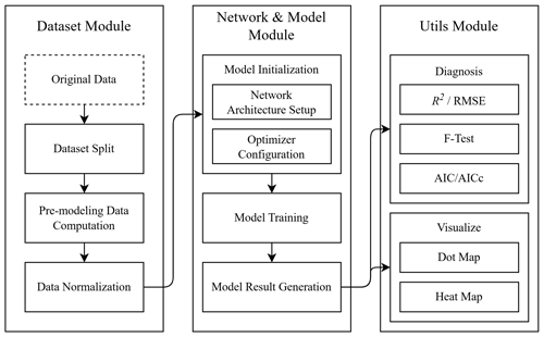
The gnnwr package is designed with a modular architecture, enabling the integration of diverse module strategies to facilitate a variety of task workflows. It comprises four primary modules: Dataset, Network, Utils, and Model.

3.1.1 Dataset

The Dataset module specifies the data types employed throughout the package. It includes the BasicDataset class for training and the PredictDataset class for prediction. This module also offers preprocessing functions that convert Pandas DataFrame data into the necessary formats (McKinney, 2010), handling tasks such as normalization and dataset partitioning. Additionally, it provides methods for saving and loading datasets, enabling users to directly work with processed data files and instantiate data objects.

3.1.2 Network

The Network module, extending PyTorch's nn.Module class, defines the architectures for models such as SWNN and STPNN. It allows users with programming expertise to customize new network structures based on existing ones, adapting to their specific research requirements.

3.1.3 Utils

The Utils module contains classes for statistical diagnostics and visualization techniques specific to spatial weighted regression. These diagnostic classes offer a suite of methods to evaluate model performance, while the visualization classes employ map-based representations to enhance the analysis of spatial data and model outcomes.

3.1.4 Model

The Model module is the cornerstone of the package, providing two classes: GNNWR and GTNNWR. GNNWR acts as the foundational class, with GTNNWR being its subclass. These classes encapsulate methods for model training, prediction, diagnostics, and loading. Users can easily invoke these methods to employ the models for problem analysis and forecasting on unseen data.

Figure 3 Workflow diagram of the package. The dashed boxes denote the raw data, the solid boxes represent the code process modules, and the arrows indicate the direction of the data flow.

3.2 Usage example for GNNWR

We commence our investigation by examining air quality modeling through the analysis of data gathered from Chinese air monitoring stations (Du et al., 2020b). This analysis seeks to delineate the spatially nonstationary associations between PM_2.5 (particulate matter with an aerodynamic diameter of less than 2.5 µm) concentrations and their environmental determinants. Given the pivotal role of PM_2.5 as an indicator of air quality, elucidating its spatial variability is crucial for comprehending the underlying spatial processes and environmental dynamics of atmospheric contamination (Han et al., 2016). The objective of this study is to develop a predictive model for the annual average PM_2.5 concentrations in the study area at a 3 km × 3 km spatial resolution for the year 2017. The model incorporates meteorological variables such as aerosol optical depth (AOD), temperature (TEMP), precipitation (TP), wind speed (WS), wind direction (WD), and elevation data (DEM).

3.2.1 Dataset initialization

Upon loading the dataset as a Pandas DataFrame, the init_dataset function from the GNNWR package is utilized to convert it into a suitable format for model input. This function randomly divides the dataset into training, validation, and testing subsets according to the ratio specified in the input parameters and computes the distance vectors for each sample, which are crucial for both model training and performance evaluation. In this specific experiment, 15 % of the data are allocated to the testing set and, out of the remaining 85 %, 10 % were used as the validation set and the rest as the training set.

In this context, it is essential to specify the independent variables, dependent variables, and spatial position variables, which correspond to the x_column, y_column, and spatial_column parameters of the init_dataset function.

When calculating the distance, the init_dataset function, by default, uses Euclidean distance to compute the spatial distances between feature points. This process generates a spatial distance vector for each point, which serves as input to the neural network component of the model. To accommodate various research requirements, the spatial_fun parameter enables users to provide a custom method for calculating spatial distances.

To optimize the speed of model training and enhance the precision of model outcomes, the function preprocesses the independent and dependent variables by default. It typically employs normalization for preprocessing; however, users have the option of adjusting the process_fun parameter to utilize standardization instead.

>>> from gnnwr.datasets import init_dataset
>>> train_set, val_set, test_set
    = init_dataset(data=data,
...               test_ratio=0.15,
...               valid_ratio=0.1,
...               x_column=x_column,
...               y_column=y_column,
...               spatial_column=spatial_column)

3.2.2 Model configuration and running

To continue, we need to create an instance of the GNNWR model. After importing the gnnwr.models module, we can do so by invoking the GNNWR class. The dense_layers parameter allows us to specify the number of hidden layers in the model's neural network, with each layer consisting of a fully connected layer, a batch normalization layer, a dropout layer, and an activation function. These hyperparameters are closely linked to the neural network's architecture, encompassing aspects such as the use of a batch normalization layer, the dropout rate, and the activation function's type. In this specific example, we have configured a neural network with a hidden layer that includes three sublayers, each with 1024, 512, 256, and 128 nodes, respectively. The activation function uses a parametric rectified linear unit (PReLU) function with an initial value of 0.2, while all the other settings are kept at their default values.

The GNNWR class uses Adadelta as its default optimizer, with an initial learning rate of 0.6, and employs a cosine annealing warm restart as its learning rate adjustment strategy. The class also supports a range of optimizers, including stochastic gradient descent (SGD), Adam, Adagrad, RMSprop, and various learning rate adjustment strategies, such as multistep and cosine annealing. These optimizers and strategies contribute to improving a model's training efficiency and performance, thereby enabling it to better accomplish its tasks.

Additionally, GNNWR involves dropout and batch normalization strategies to avoid overfitting and improve the generalizability and performance of the model. The default dropout rate is 0.2 and can be altered through the drop_out parameter. The model applies batch normalization by default, which can be disabled by setting the batch_norm parameter to False.

To streamline the model training, we can utilize the run function to specify the number of iterations and the frequency of printing training process information, allowing us to monitor training progress and performance. Throughout the training process, we will retain the best-performing model within the validation set to prevent the GNNWR model from overfitting. Selecting the optimal model helps minimize the expected error and guarantees that the model will possess superior generalization ability. For storage convenience, the model repository will only retain a file containing the neural network components of the model. This file encapsulates the structural configuration and parameter information of the neural network.

>>> from gnnwr import models
>>> from torch import nn
>>> gnnwr = models.GNNWR(train_dataset = train_set,
...                      valid_dataset = val_set,
...                      test_dataset = test_set,
...                      dense_layers = [1024, 512, 256, 128],
...                      activate_func = nn.PReLU(init=0.2),
...                      start_lr = 0.6,
...                      optimizer = "Adadelta",
...                      drop_out = 0.2,
...                      batch_norm = True,
...                      model_name = "GNNWR_PM25")
>>> gnnwr.run(max_epoch = 2000, print_frequency = 500)

The GNNWR package uses TensorBoard to record the model training process, including the loss and R² scores on the training and validation sets for each epoch as well as the learning rate and best R² scores obtained on the validation set. By observing the changes in the model during the training process, targeted adjustments to the training method can be made. To enhance users' comprehension of the model architecture, we have incorporated the add_graph function. When utilized, this function enables users to visualize the structure of the model within the “Graphs” section of TensorBoard. This functionality not only clarifies the model's architecture but also facilitates the prompt identification of issues during model debugging and optimization, thereby substantially improving model performance.

3.2.3 Results and visualization

We can obtain the composition and results of the model through the result method, which includes the model structure, optimizer structure, and used variables as well as the accuracy, complexity, and content of the statistical tests performed on the model. Among them, the R² and RMSE (root mean square error) indicators summarize the model's fitting ability, while the Akaike information criterion (AIC) and corrected AIC (AICc) indicators provide a deeper understanding of the model's complexity. The F₁, F₂, and F₃ statistical data are used as sample diagnostic measures (Wu et al., 2019). The first two values indicate the presence of significant spatiotemporal nonstationarity in the model, while the last value evaluates the significance of spatiotemporal nonstationarity in the regression parameters of each independent variable.

>>> gnnwr.result()

--------------------Model Information-----------------
Model Name:           | GNNWR_PM25
independent variable: | ['dem', 'w10', 'd10', 't2m', 'aod_sat', 'tp']
dependent variable:   | ['PM2_5']

OLS coefficients:
x0: 7.12861
x1: -4.03670
x2: -1.90988
x3: 21.29951
x4: 36.57638
x5: -24.50677
Intercept: 19.16957

--------------------Result Information----------------
Test Loss: |                  33.42091
Test R2  : |                   0.84280
Train R2 : |                   0.84762
Valid R2 : |                   0.84541
RMSE: |                        5.78108
AIC:  |                     1257.37056
AICc: |                     1254.68787
F1:   |                        0.11974
F2:   |                        3.52673
f3_param_0: |                  1.81630
f3_param_1: |                 19.05118
f3_param_2: |                  0.42682
f3_param_3: |                 68.13538
f3_param_4: |                 47.61187
f3_param_5: |                170.05663
f3_param_6: |                122.83797

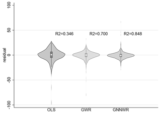
The empirical results reveal that the model exhibits robust performance in the reconstruction of PM_2.5 distributions, and the statistical analyses confirm the presence of significant spatial heterogeneity in PM_2.5 concentrations. In terms of statistical indicators, the model achieved R² scores of 0.848 for the training dataset, 0.845 for the validation dataset, and 0.843 for the test dataset, which are much higher than traditional models like OLS and GWR (implemented with the mgwr package by Oshan et al., 2019, version 2.2.1). Also, the residuals of GNNWR are generally smaller than those of traditional models, with most residuals being close to zero and rarely showing large deviations (Fig. 4). Such outstanding performance reflects GNNWR's ability to capture complex patterns in spatiotemporal data, demonstrating the effectiveness of introducing the nonlinear fitting ability of neural networks when modeling spatial nonstationarity.

It is noteworthy that, as a deep-learning model, GNNWR requires more time than traditional models to fit the given dataset. For the above experiment on the PM_2.5 dataset, it takes 2000 epochs for GNNWR to optimize the network's parameters and minimize the loss, which is about 3 min in a CPU (Intel Core i5-12400) environment. Nevertheless, compared to the advantages in model performance, such time consumption is acceptable, especially considering that a CUDA-enabled GPU can further accelerate the process.

Figure 4 The residual distributions and R² indicator for OLS, GWR, and GNNWR in the PM_2.5 dataset.

Owing to the intimate association between model analysis and spatial aspects, GNNWR furnishes a range of spatial visualization functionalities grounded in the folium. By instantiating the Visualize object, we can render various model variables within a spatial context. The Visualize object offers multiple visualization techniques encompassing the visualization of internal datasets within the model, heatmaps of coefficients, and the visualization of spatial points. Figure 5 illustrates the spatial distribution of the dependent variable PM_2.5 across the dataset. Notably, PM_2.5 concentrations are elevated in the North China and Xinjiang regions, in contrast to the relatively lower levels observed in Yunnan and the northern reaches of Inner Mongolia.

>>> import gnnwr.utils as utils
>>> visualizer = utils.Visualize(data=gnnwr,
    lon_lat_columns=['lng','lat'])
>>> visualizer.display_dataset(name='all',y_column='PM2_5')

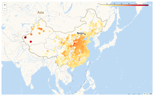
Figure 5 Diagram of the spatial distribution of PM_2.5. Redder points represent higher PM_2.5 values. Map crafted using Python's folium library with the Gaode basemap. Publisher's remark: please note that the above figure contains disputed territories.

The coefs_heatmap function facilitates the visual representation of the spatial distribution of independent variable coefficients, thereby enriching our comprehension of the impact of individual independent variables on the dependent variable across varying geographical contexts. Figure 6 depicts the distinctive spatial distribution patterns of AOD coefficients.

>>> visualizer.coefs_heatmap('coef_aod_sat')

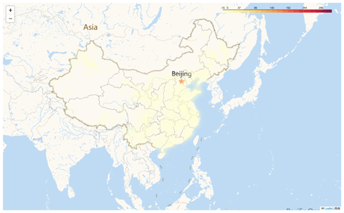
Figure 6 Diagram of the AOD coefficient distribution. Darker areas highlight regions with strong positive correlations, indicating high levels of particulate matter. Map crafted using Python's folium library with the Gaode basemap. Publisher's remark: please note that the above figure contains disputed territories.

Through these visualization techniques, we can perceptively comprehend the analysis outcomes of the model. They offer abundant functionality that enables us to better understand the spatial behavior of the model and gain a more profound insight into the model's performance and spatial relationships.

Concurrently, the visualization output of the Visualize object is in HTML format, permitting researchers to manipulate the map via zooming, panning, and rotation. During the manipulation of the map, the visualization of the data will change according to the scale of the map. When the map scale is small, the points in the spatial distribution are dense, necessitating the clustering and display of these points to preserve clarity. Conversely, when the map scale is large, the information of the points at specific locations will be displayed. This facilitates detailed inspection and analysis of geographic data to cater to diverse research requirements.

3.2.4 Saving and reusing

Upon successful completion of model training, a frequent need arises to reuse said model. To facilitate this process, the model repository incorporates a dedicated load_model function, which is specifically purposed to reload model files that were automatically saved during the training progression. Notably, the repository only retains the neural-network-related components, specifically the neural network architecture and parameters, within the model. Consequently, when reusing a model, the recommended sequence is as follows: initially, construct an instance corresponding to the model's architectural design before subsequently calling the load_model method to import the parameters and weights.

3.2.5 Prediction

Ultimately, we can employ the prediction method to forecast other datasets. Prior to generating predictions, it is essential to transform the other datasets into the predictDataset class, which is integrated within the GNNWR package. This transformation can be accomplished by utilizing the init_predict_dataset method. This method computes the distance vectors between the features in the dataset to be predicted and the reference points and applies the identical scaling transformation to the independent variables as in the training dataset, guaranteeing that the input for the model inference will follow the same statistical distribution as the training data. The prediction method yields a Pandas DataFrame comprising the original data and the predicted results. Moreover, when employing the GNNWR model for analysis, spatial weights are of paramount importance. These weights signify the spatial variability of the influence of each independent variable on the dependent variables. To acquire spatial weights, the predict_weight method can be utilized to output pertinent information. Figure 7 presents a geographical visualization of the GNNWR model's predictive outcomes.

>>> from gnnwr.datasets import init_predict_dataset
>>> pred_dataset = init_predict_dataset(data = pred_data,
...                                     train_dataset = train_set,
...                                     x_column=x_column,
...                                     spatial_column=spatial_column)
>>> res = gnnwr.predict(pred_dataset)

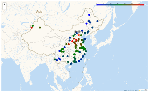
Figure 7 Geospatial visualization of GNNWR model predictions for PM_2.5. The red points indicate higher PM_2.5 predictions; the blue points indicate lower PM_2.5 predictions. Map crafted using Python's folium library with the Gaode basemap. Publisher's remark: please note that the above figure contains disputed territories.

Figure 8 The residual distributions and R² indicator for OLS, GTWR, and GTNNWR in the DSi dataset.

3.3 Usage example for GTNNWR

The workflow of employing GTNNWR is largely akin to that of the GNNWR model. We exemplify this by utilizing daily surface dissolved silicate (DSi) concentration data from the offshore waters of Zhejiang. This study utilized the GTNNWR approach to retrieve the distribution of coastal DSi concentrations, addressing the challenges posed by spatiotemporal nonstationarity (Qi et al., 2023).

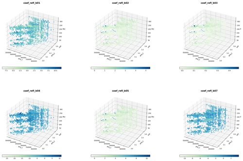
Figure 9 Model coefficients in a 3D space–time coordinate system. The blue dots represent a greater positive effect of the variable on the silicate concentration; the lighter dots represent a smaller effect.

3.3.1 Dataset initialization

Similar to the GNNWR model, data preprocessing is essential when utilizing the GTNNWR model to acquire a data format that the model can process as well. The GTNNWR model is specifically tailored for spatiotemporal data, wherein the regression coefficients perpetually vary in both space and time. Consequently, the data processed by the model must possess spatiotemporal attributes. When employing the init_dataset function, designating the time data as the time dimension can generate valid input for the GTNNWR model. This function computes the time distance vectors based on the distance calculation method specified by the temporal_fun parameter and subsequently employs them as input features for each sampling point. The default time distance calculation method is the Manhattan distance.

>>> train_set, val_set, test_set = init_dataset(data=data,
...                                             test_ratio=0.15,
...                                             valid_ratio=0.1,
...                                             x_column=x_column,
...                                             y_column=y_column,
...                                             spatial_column=spatial_column,
...                                             temp_column=temp_column)

3.3.2 Model configuration and running

GTNNWR is designed as a subclass incorporated within the GNNWR package, inheriting from its foundational GNNWR class. As a result, it retains the same set of methods inherent to its superclass. The instantiation process for the GTNNWR model closely mirrors that of GNNWR, with the primary difference lying in the input format for hidden layers – a two-element, two-dimensional list. This unique input configuration stems from GTNNWR's integration strategy, which involves employing a STPNN to compute spatiotemporal proximities and then feeding these computations into a STWNN to determine spatiotemporal weights. Specifically, the first list in this input designates the hidden-layer structure of STPNN, whereas the second list delineates the hidden-layer architecture pertaining to STWNN.

The procedure for training an instantiated model with data, together with the tasks of printing model metadata and exhibiting the outcomes of the training, aligns with the methodologies employed in the previous example.

>>> optimizer_params = {
...     "maxlr": 0.025,
...     "minlr": 0.010,
...     "upepoch": 1000,
...     "decayepoch": 2000,
...     "decayrate": 0.998,
...     "stop_change_epoch": 5000,
...     "stop_lr": 0.01,
... }
>>> Layers = [[3], [1024, 512, 256,128,64,32]]
>>> gtnnwr = models.GTNNWR(train_set, val_set, test_set,
...                        Layers,
...                        optimizer='SGD',
...                        optimizer_params=optimizer_params,
...                        # drop_out=0.3,
...                        model_name="GTNNWR_DSi",
...                        model_save_path="./demo_result/gtnnwr_models",
...                        log_path="./demo_result/gtnnwr_logs/",
...                        write_path="./tf-logs/gtnnwr_runs")
>>> gtnnwr.run(max_epoch = 4000)
>>> gtnnwr.result()

--------------------Model Information-----------------
Model Name:           | GTNNWR_DSi
independent variable: | ['refl_b01', 'refl_b02', 'refl_b03', 'refl_b04',
                         'refl_b05', 'refl_b07']
dependent variable:   | ['SiO3']

OLS coefficients:
x0: 6.84114
x1: 1.63606
x2: 0.11273
x3: -5.76276
x4: 1.62136
x5: -2.69205
Intercept: 1.05858

--------------------Result Information----------------
Test Loss: |                   0.16574
Test R2  : |                   0.68628
Train R2 : |                   0.71628
Valid R2 : |                   0.75261
RMSE: |                        0.40711
AIC:  |                      460.66438
AICc: |                      463.34515
F1:   |                        0.22449
F2:   |                      -12.20421
f3_param_0: |                 27.02276
f3_param_1: |                  0.12710
f3_param_2: |                  0.94117
f3_param_3: |                  2.37350
f3_param_4: |                 17.69786
f3_param_5: |                 28.23304
f3_param_6: |                267.06781

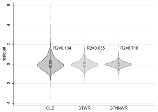
According to various model indicators, utilizing neural networks to estimate the spatiotemporal nonstationarity of DSi is indeed effective. The model successfully achieved R² values of 0.716, 0.752, and 0.686 in the training, validation, and testing sets, respectively, effectively reconstructing the distribution of silicate in the offshore waters of Zhejiang. As indicated by Fig. 8, such coefficients of determination are much higher than those of traditional models like OLS and GTWR (implemented with the mgtwr package by Sun, 2024, version 2.0.5); also, the residuals of GTNNWR are generally smaller than those of OLS and GTWR. These outstanding performances demonstrate GTNNWR's superior performance in capturing the spatiotemporal nonstationarity of DSi concentrations.

3.3.3 Results and visualization

In order to investigate the variability of coefficients for distinct variables across different samples, one can leverage the reg_result function. The function computes and systematically arranges each sample's coefficient values into a Pandas DataFrame format, thereby outputting the results. With the resulting coefficient matrix in hand, researchers can then conduct targeted analyses pertinent to specific spatial processes. For instance, we can visualize the coefficients of each variable by employing time and space as three-dimensional coordinate axes (Fig. 9). This enables us to directly observe the relationship between the bands of remote sensing images and silicate concentrations at different spatial locations. By integrating relevant prior knowledge, we can interpret the outcomes of the model.

4 Conclusions

This study introduces the GNNWR package, a Python-based model repository designed to facilitate spatiotemporal intelligent regression modeling. The package is constructed on PyTorch, a widely employed deep-learning framework, and affords a comprehensive workflow for simulating geographical processes characterized by spatiotemporal nonstationarity. The GNNWR package optimizes intricate procedures encompassing data preprocessing, network architecture formulation, model training, and result computation, thereby enhancing user accessibility. It enables individuals with limited programming expertise to quickly master the application of pertinent models such as GNNWR and GTNNWR for the estimation of spatiotemporal nonstationary processes. The integrated visualization functionalities further augment the package's utility, allowing users to interpret model outcomes and their spatial relationships more effectively.

However, the GNNWR package is not without its limitations. The GNNWR and GTNNWR models are computationally intensive, particularly for large datasets. Also, training neural networks requires substantial computational resources, which may limit accessibility for some users. Future works should focus on the following: optimizing computational efficiency, implementing parallel processing techniques, and optimizing model architectures are potential methods that can significantly reduce computation times. Data handling is another area that can be improved: incorporating techniques for spatiotemporal data augmentation and preprocessing can make models more robust and applicable to a wider range of datasets.

In addition, scholarly understanding of spatiotemporal nonstationarity is progressing, driving the continual evolution of GNNWR-based models and the emergence of diverse derivatives, such as geographically convolutional neural-network-weighted regression (Dai et al., 2022) and directional geographically weighted neural network regression (Wu et al., 2019). These model variants have substantially augmented the functionalities of GNNWR across various dimensions. Moving forward, we are committed to enhancing the model library by leveraging the current framework and integrating a variety of network and data architectures to create novel extension models. This expansion will enhance the package's ability to incorporate a wide range of modeling techniques for addressing spatiotemporal nonstationarity. Consequently, this broadening of capabilities will extend the applicability of the models, encompassing a more comprehensive array of spatiotemporal analytical approaches.