Do data-driven models beat numerical models in forecasting weather extremes? A comparison of IFS HRES, Pangu-Weather, and GraphCast

The last few years have witnessed the emergence of data-driven weather forecast models capable of competing with – and, in some respects, outperforming – physics-based numerical models. However, recent studies have questioned the capability of data-driven models to provide reliable forecasts of extreme events. Here, we aim to evaluate this claim by comparing the performance of leading data-driven models in a semi-operational setting, focusing on the prediction of near-surface temperature and wind speed extremes globally. We find that data-driven models mostly outperform ECMWF’s physics-based deterministic model in terms of global RMSE for forecasts made 1–10 d ahead and that they can also compete in terms of extreme weather predictions in most regions. However, the performance of data-driven models varies by region, type of extreme event, and forecast lead time. Notably, data-driven models appear to perform best for temperature extremes in regions closer to the tropics and at shorter lead times. We conclude that data-driven models may already be a useful complement to physics-based forecasts in regions where they display superior tail performance but note that some challenges still need to be overcome prior to operational implementation.

1 Introduction

The first deep learning models for weather applications date back to the 1990s (Schizas et al., 1991; Hall et al., 1999), but it is only in recent years that deep learning models have become competitive as self-standing medium-range forecasting tools. Since 2022, at least eight different research groups (Pathak et al., 2022; Bi et al., 2023; Keisler, 2022; Lam et al., 2023; Chen et al., 2023a; Nguyen et al., 2023; Chen et al., 2023b; Lang et al., 2024) have claimed to have developed deep learning models capable of producing more accurate deterministic forecasts compared to those from the state-of-the-art physics-based models of the European Centre for Medium-Range Weather Forecasts (ECMWF) across a range of atmospheric variables over multiple lead times. Recent independent studies (Rasp et al., 2024; Bouallègue et al., 2024) support these claims, showing how data-driven models can outperform physics-based models across a wide range of parameters and metrics. In particular, WeatherBench 2 (Rasp et al., 2024) provides comprehensive global and regional scorecards for comparing forecast models in terms of RMSE while also making all test predictions produced freely available to the public.

However, the studies conducted so far have focused on the average skill of the forecasts, without any special treatment of extreme events. Even though some cases studies have been conducted – for instance, on cyclone tracking (Charlton-Perez et al., 2024; Bi et al., 2023; Lam et al., 2023; Chen et al., 2023b) and surface temperature extremes (Bouallègue et al., 2024; Lam et al., 2023) – these are too limited to allow for a fair assessment of the capacity of data-driven models to forecast weather extremes globally. The timely and reliable forecasting of weather extremes plays a key role in disaster management and risk mitigation (World Meteorological Organization, 2022; Merz et al., 2020), as well as in crucial socio-economic functions, such as those of the energy and insurance sectors (e.g. Kron et al., 2019). We thus argue that greater emphasis should be placed on understanding whether data-driven models can provide reliable forecasts of weather extremes before such models are implemented operationally (Watson, 2022).

In addition, recent studies (Watson, 2022; Olivetti and Messori, 2024; de Burgh-Day and Leeuwenburg, 2023) problematise the assumption that strong performance in standard metrics of average skill should translate by default into an equally strong performance in the tails of the distribution. Indeed, there may be several reasons for an asymmetry between average skill and skill for extremes, including the intrinsic sparsity of extreme events in training datasets (Watson, 2022), the use of symmetric loss functions that are inadequate for extremes (Xu et al., 2024; Olivetti and Messori, 2024), and the multi-task and multi-step optimisation approaches used in leading deep learning architectures (e.g. Bi et al., 2023; Lam et al., 2023). These issues are further exacerbated by the fact that the current generation of data-driven models published in peer-reviewed journals provide deterministic predictions, even though a number of promising approaches for providing uncertainty estimates for these predictions exist for older data-driven models (e.g. Scher and Messori, 2021; Clare et al., 2021) and are currently being explored for state-of-the-art models (e.g. Price et al., 2024; Hu et al., 2023; Bi et al., 2023; Zhang et al., 2023; Cisneros et al., 2023; Guastavino et al., 2022; Kashinath et al., 2021).

This article aims to evaluate whether deep learning models can provide skilful forecasts of extreme weather by providing a pragmatic comparison between physics-based and data-driven models in a semi-operational setting. Specifically, it compares the performance of ECMWF's IFS HRES with that of leading global deep learning models in forecasting near-surface temperature and wind speed extremes 1–10 d ahead when provided with the same set of inputs, namely the output of IFS HRES at time 0. To do so, it makes use of the freely available forecast data provided by ECMWF and the WeatherBench 2 dataset (Rasp et al., 2024). The methods for the comparisons between models are largely based on the guidelines for the evaluation of tail performance provided by Watson (2022): (i) comparisons are given in terms of a standard metric (RMSE) computed on data beyond extreme quantiles only, (ii) visual assessment of performance is conducted on extremes for specific regions/grid points, and (iii) quantile–quantile plots of extreme quantiles are used to identify possible inconsistencies in tail estimation. All comparisons are performed at multiple timescales (1–10 d) and for the whole globe, with separate metrics for each region following the ECMWF operational scorecards (ECMWF, 2024).

In the next two sections, we provide an introduction to the models included in the evaluation and the methods employed for the comparison. Then, we outline the results of the comparison for all the variables and regions of interest. Lastly, we reflect on the results of these comparisons and on how they may affect the operational implementation of data-driven models. Additional results for models using ERA5 reanalysis data (Hersbach et al., 2020) as input are included in Appendix D.

2 Models and methodology

The rationale behind the choice of models and the methodology employed is to make the comparison between data-driven models and physics-based models as fair as possible. For this reason, we include in the main text only those data-driven models from WeatherBench 2 that are able to take the same set of initial conditions as IFS HRES, ECMWF's high-resolution deterministic forecasting system. All the models discussed in the main text therefore take IFS HRES at time 0 as input and are able to produce 6-hourly forecasts of 2 m temperature and 10 m wind, the variables according to which the models are evaluated in this paper. These outputs are, in turn, compared to the same ground truth, ERA5 (Hersbach et al., 2020), at a 1.5° horizontal resolution, as in WeatherBench 2 (Rasp et al., 2024). Indeed, models taking reanalysis data as input present a conceptual difference from operational models as they are based on input data that are available with a considerable time delay and thus cannot be used in an operational setting.

Two data-driven models fit the criteria established above: the operational Pangu-Weather (Bi et al., 2023) and GraphCast (Lam et al., 2023) models. We believe these models may reasonably represent the overall performance of deterministic data-driven models since they display performance similar to that of other data-driven models across a range of atmospheric and surface variables over multiple lead times (Rasp et al., 2024). Furthermore, these models employ the two leading architectures for deterministic data-driven weather forecasting, namely vision transformers (Dosovitskiy et al., 2020) and graph neural networks (Scarselli et al., 2009). Yet, recognising that some subtle differences may be lost by not including a more diverse range of data-driven models in our comparison, we present in Appendix D a comparison between IFS HRES and reanalysis-based deep learning models – specifically, reanalysis-based Pangu-Weather and GraphCast models, as well as FuXi (Chen et al., 2023b). These are currently regarded as the best deterministic data-driven models in terms of RMSE for medium–long-range forecasting (Rasp et al., 2024).

In this section, we first provide a brief description of each of the models included in the comparison in the main text and then outline the criteria on which the comparison is based. For a complete description of the models, including a full list of inputs and outputs, we refer the reader to Rasp et al. (2024) and Olivetti and Messori (2024), as well as to the original papers introducing the models described in Sect. 2.1–2.3.

2.1 IFS HRES

IFS HRES is ECMWF's flagship deterministic high-resolution model and is widely regarded as one of the best physics-based numerical-weather-forecast models in the world (Rasp et al., 2020, 2024). All the parameters included in the model, as well as its regular updates and improvements, are thoroughly documented on ECMWF's website (Blanchonnet, 2022). Currently, IFS HRES takes a much larger set of inputs than any of the data-driven models. It also produces hourly forecasts for a very large set of outputs and does so at a 0.1° horizontal resolution across 137 pressure levels. The inputs forming IFS HRES's initial conditions (IFS HRES at time 0) are a mix of in situ observations from the 3 h surrounding the forecast and model outputs from the previous IFS HRES run. IFS HRES is included here as the baseline to which the performance of the data-driven models is compared. All IFS HRES forecasts were generated with the operational version of the model used at the time of the forecast (Rasp et al., 2024), i.e. the model configuration Cy46r1 for forecasts initiated before 30 June 2020 and Cy47r1 for forecasts initiated after that date.

2.2 Pangu-Weather

Pangu-Weather (Bi et al., 2023) is a data-driven deep learning model using a vision transformer architecture (Dosovitskiy et al., 2020). First developed in 2022 (Bi et al., 2022) and published in 2023 (Bi et al., 2023), it is the oldest data-driven model among those included in the comparison. It is trained on ERA5 reanalysis data from 1979 to 2017 and uses 2018–2019 for validation. It takes as input five upper-air variables from 13 atmospheric levels and four surface variables, and it produces forecasts of these variables for the next atmospheric state 6 h ahead in a sequential manner. The output of the model can then be fed in again as input to obtain forecasts at longer lead times. In this way, it is possible to obtain forecasts up to 10 d ahead at a 0.25° resolution. In its operational version, analysed in the main text here, Pangu-Weather takes IFS HRES at time 0 as input, while the version included in Appendix D takes ERA5 as an initial state. The operational and reanalysis-based versions of Pangu-Weather are otherwise identical.

2.3 GraphCast

GraphCast (Lam et al., 2023) is a deep learning model using a graph-based architecture (Scarselli et al., 2009). First developed in late 2022 (Lam et al., 2022) and published in Lam et al. (2023), it builds on earlier work by Keisler (2022). It is trained on ERA5 reanalysis data from 1979 to 2019 and, in the operational version, is additionally fine-tuned on a smaller sample of IFS HRES data. It takes as input six atmospheric variables from 37 atmospheric levels, as well as numerous surface variables and masks. GraphCast aims to forecast the next state of the atmosphere as a function of its two previous states in a sequential manner. Like Pangu-Weather, it produces 6-hourly forecasts up to 10 d ahead at a 0.25° resolution. The main difference between the operational version analysed in the main text and the version included in Appendix D is that the operational version does not require precipitation as input, thus allowing for the use of IFS HRES at time 0 as input.

2.4 Criteria for model comparison

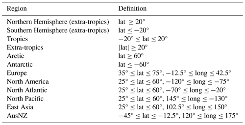
The comparison between models is based on their performance in forecasting cold and hot extremes in 2 m temperature and 10 m wind speed extremes globally. Following WeatherBench 2 (Rasp et al., 2024), the models are tasked with making forecasts with a time step of 6 h or less, and all comparisons are based on a spatial resolution of 1.5°. Forecasts are initiated every 12 h (00:00 and 12:00 UTC) for the period from 1 January 2020 to 16 December 2020, thus providing 702 comparable forecasts for each lead time and grid point. Comparisons are performed globally and for regions included in the ECMWF operational scorecards (ECMWF, 2024), as defined in Table 1.

Table 1 Regions for forecast performance evaluation, in accordance with ECMWF's operational scorecards (ECMWF, 2024). AusNZ: Australia and New Zealand.

For the sake of conciseness, we focus our comparison here on forecasts for 1, 3, 5, 7, and 10 d ahead. We evaluate the performance of the models based on three different criteria, largely based on the recommendations for the evaluation of extreme event forecasts provided by Watson (2022). The criteria are as follows:

• 1.

  Accuracy in determining the magnitude of the most extreme data points is assessed globally or within a given region. To define the extremes, we pool together all data points for 2020 for the region of choice and set a threshold based on a quantile of choice from all the data points. We then consider all data points exceeding this threshold to be extreme. Accordingly, we allow any number of global and regional extremes to come from a specific grid point or time. The number of data points used for evaluation in each region is thus calculated by multiplying 702 (the data points at each grid point) by the number of grid points within the specific region and then multiplying the result by the percentage of data points exceeding the chosen quantile-based threshold. For example, if the top 5 % of events were considered, the number of data points for evaluation would be calculated by multiplying 702 by the number of grid points in the region and then multiplying the result by 0.05. Accuracy is measured in terms of RMSE (lower values are better), as defined below:

  • For hot and wind speed extremes,

    $$\begin{array}{}\text{(1)}& \begin{array}{rl}& {\mathrm{RMSE}}_t\\ & =\sqrt{{\displaystyle \frac{\mathrm{1}}{TIJ}}\sum _t^T\sum _i^I\sum _j^{J}w\left(i\right){\mathrm{1}}_{o_t>Q\left(o\right)}({\widehat{y}}_{t,i,j}-o_{t,i,j}{)}^{\mathrm{2}}}\end{array}.\end{array}$$

  • For cold extremes,

    $$\begin{array}{}\text{(2)}& \begin{array}{rl}& {\mathrm{RMSE}}_t\\ & =\sqrt{{\displaystyle \frac{\mathrm{1}}{TIJ}}\sum _t^T\sum _i^I\sum _j^{J}w\left(i\right){\mathrm{1}}_{o_t<Q\left(o\right)}({\widehat{y}}_{t,i,j}-o_{t,i,j}{)}^{\mathrm{2}}},\end{array}\end{array}$$

    where $\mathrm{1},\mathrm{2},\mathrm{3},\mathrm{\dots },T$ represents the available number of time points for the given forecast lead time (T is 702 in our case). Moreover, $\mathrm{1},\mathrm{2},\mathrm{3},\mathrm{\dots },I$ represents the number of points of latitude included in the region of interest; $\mathrm{1},\mathrm{2},\mathrm{3},\mathrm{\dots },J$ represents the number of points of longitude included in the region of interest; $\widehat{y}$ is the forecasted value of the variable of interest; o is the observed value of the variable of interest (from ERA5 in our case); and ${\mathrm{1}}_{o_t>Q\left(o\right)}$ is an indicator function that takes a value of 1 for data points above the chosen quantile of the variable of interest in the given region and takes a value of 0 otherwise. For cold extremes, ${\mathrm{1}}_{o_t<Q\left(o\right)}$ so that the indicator function takes a value of 1 for data points below the chosen quantile and takes a value of 0 otherwise. Differences in performance between models are assessed for significance at the 5 % level using a paired t test with cluster-robust standard errors (Liang and Zeger, 1986; Arellano, 1987; Cameron and Miller, 2015), which accounts for the spatial and temporal clustering of extreme events. The test is conducted in a two-sided manner when comparing data-driven models with IFS HRES and in a one-sided manner when specifically assessing whether the best individual model significantly outperforms the second-best model within a specific region.

• 2.

  Accuracy in determining the magnitude of grid-point extremes is considered. Extremes are defined as in criterion 1 (but at the grid-point level) by defining a different threshold and set of extremes for each grid point. The RMSE is computed according to Eqs. (1) and (2), with a redefined indicator function. For hot extremes, the indicator function is given by ${\mathbb{1}}_{o_{t,i,j}\ge Q\left(o_{i,j}\right)}$, taking a value of 1 for data points above or equal to the quantile of interest at the given point of latitude and longitude and taking a value of 0 otherwise. For cold extremes, the indicator function becomes ${\mathbb{1}}_{o_{t,i,j}\le Q\left(o_{i,j}\right)}$. Thus, the number of data points available at each grid point is calculated by multiplying 702 by the percentage of data points exceeding the chosen quantile.

  Grid-point-level differences in performance between the best data-driven model and IFS HRES are assessed for significance using the same approach as that used in criterion 1. The obtained p values are corrected for multiple testing by applying global false-discovery rates (Benjamini and Hochberg, 1995; Wilks, 2016) using a global significance level of 0.1. This corresponds to an approximate significance level of 0.05 in the presence of strongly spatially correlated events (Wilks, 2016), such as near-surface temperature extremes.

• 3.

  Calibration of extreme quantiles, where quantile behaviour closer to the ground truth (ERA5) is considered superior to quantile behaviour further away from it, is assessed. We evaluate extreme quantile behaviour by considering quantiles between 90 and 99.9 for hot and wind extremes and quantiles between 10 and 0.1 for cold extremes. We then produce quantile–quantile plots in which the extreme quantiles from the forecasts are plotted against the corresponding quantiles from ERA5.

  The three criteria jointly provide an overall picture of the performance of the models in forecasting near-surface temperature and wind extremes at both global and regional levels (criterion 1), as well as at the local level (criterion 2), along with insights into the tail behaviour of the models when confronted with values at the edges or beyond the limits of the training distribution (criterion 3).

3 Results

In this section, we report the results of the model comparison performed according to the criteria outlined in Sect. 2.4. The aim here is both to provide a comprehensive comparison between data-driven and physics-based models and to identify relevant differences between the data-driven models themselves.

We start by providing an overview of the performance of different models globally and in individual regions, considering all data points – both extreme and non-extreme. For all models, performance differences between regions are small, especially for 10 m wind speed (Fig. 1). Both data-driven models perform significantly better than ECMWF's IFS HRES globally and in most regions. Most impressively, GraphCast significantly outperforms IFS HRES across all regions and lead times.

The difference between GraphCast and Pangu-Weather is smaller overall, with the largest differences observed in 2 m temperature forecasts at longer lead times. Notably, GraphCast consistently outperforms Pangu-Weather across all regions in these longer-range forecasts, with differences in the range of 5 % to 20 % for 10 d forecasts of 2 m temperature. The strong performance of GraphCast may partly depend on its training scheme, which assigns additional weight to surface and lower-tropospheric variables at the expense of higher atmospheric levels (Lam et al., 2023).

The performance of the data-driven models, especially that of Pangu-Weather, appears to deteriorate at a faster rate than that of IFS HRES at longer lead times. This might be a sign that data-driven models suffer from “blurring” (Bonavita, 2024; Price et al., 2024) – namely, the tendency to revert to the climatology and produce progressively less skilful forecasts with increasing lead time. While this problem applies to both physical and data-driven models, it has recently been shown to be prominent among data-driven models (Bonavita, 2024).

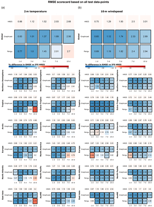
Figure 1 RMSE scorecards for 2 m temperature (a) and 10 m wind speed (b) at global and regional scales, computed on all test data points. Blue shades indicate performance better than that of IFS HRES, while red shades indicate worse performance. Black borders indicate significantly different performance compared to IFS HRES (at the 5 % level). AusNZ: Australia and New Zealand.

Figure 2 provides RMSE comparisons for the most extreme 5 % of data points globally and in each region, in accordance with criterion 1 (Sect. 2.4). Globally, GraphCast significantly outperforms IFS HRES across all three categories over most lead times, with the largest differences noted for hot and windy extremes. Pangu-Weather performs more similarly to IFS HRES, with statistically significant improvements in performance observed only for hot extremes at shorter lead-times (1–3 d ahead) and worse performance than IFS HRES noted for hot and windy extremes at longer lead times.

Similar to the trends observed for all data, the performance of both data-driven models on extremes degrades compared to that of IFS HRES for longer forecast lead times. This is particularly notable for predictions made 10 d ahead. This is perhaps not surprising given that the 10 d predictions are close to the limits of skilful forecasting for extremes. However, this may also be interpreted as an additional sign of blurring. The fact that the data-driven models incorporate the iterative feeding of the most recent atmospheric states to generate one-step-ahead forecasts may also play a role in this respect. Indeed, this approach may contribute to the accumulation of small errors over time, which become more relevant for extreme weather forecasts at longer lead times (Bonavita, 2024).

Regional comparisons between models largely confirm the aforementioned patterns while also revealing some additional details. Overall, data-driven models demonstrate better performance relative to IFS HRES in the Northern Hemisphere than in the Southern Hemisphere, particularly for cold extremes. Notably, IFS HRES significantly outperforms both data-driven models in AusNZ (Australia and New Zealand) and Antarctica with respect to cold extremes, as well as in East Asia, North America, and Antarctica with respect to hot extremes. The comparatively poor performance of the data-driven models in Antarctica may be attributed to the lower quality of reanalysis data for this region, which is the basis on which the data-driven models are trained.

Conversely, GraphCast outperforms IFS HRES in the tropics and the North Pacific across all variables over all lead times and outperforms IFS HRES in the Arctic with respect to temperature extremes. We speculate that some of these regional differences may be attributed to the lack of input variables relevant to near-surface extremes (e.g. soil moisture and snow and ice cover) in the training of data-driven models; these variables might play a more prominent role in certain regions than in others (e.g. soil moisture with respect to hot extremes in continental North America and East Asia (Coronato et al., 2020; Liu et al., 2014)).

Additionally, we observe that in most regions, data-driven models perform better for temperature than for wind extremes relative to IFS HRES. A possible reason for this might be the lack of specific training on 10 m wind speed for GraphCast and Pangu-Weather, which are instead trained on u- and v-wind components separately. This approach may be suboptimal for wind speed extremes as the non-linear relationship between errors in the individual wind components and the resultant total wind speed can lead to large errors in wind speed forecasts. Even a small underestimation in one wind component can result in a substantial underestimation of total wind speed under strong wind conditions.

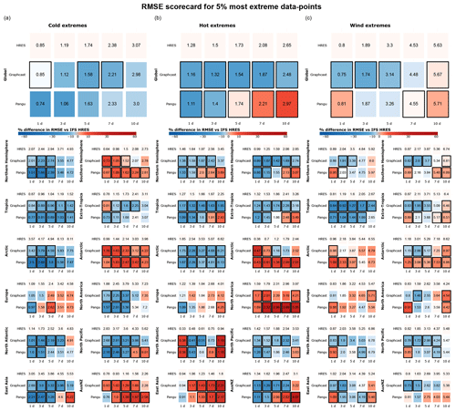
Figure 2 RMSE scorecards for (a) cold, (b) hot, and (c) wind extremes at global and regional scales, computed on (a) the lowest 5 % of data points for 2 m temperature, (b) the highest 5 % of data points for 2 m temperature, and (c) the highest 5 % of data points for 10 m wind speed. Black borders indicate statistically significant differences in performance compared to IFS HRES (at the 5 % level).

Figure 3 repeats the analysis presented in Fig. 2 but instead considers the most extreme 1 % of data points in each region. The conclusions drawn from Fig. 3 largely hold for wind and hot extremes but not necessarily for cold extremes. Specifically, there is a noticeable decline in the performance of data-driven models, particularly GraphCast, with respect to cold extremes, both globally and in the extra-tropics. However, it is important to consider that our approach to selecting extremes may result in a higher proportion of global cold extremes originating from Antarctica in Fig. 3 than in Fig. 2. This could explain the worse performance of the data-driven models, given their relatively weak performance in this region.

Additionally, we observe larger regional differences in Fig. 3 than in previous figures. This may be the result of the smaller sample size and the larger variability associated with a smaller number of extreme events. The difference in performance between the Northern and Southern hemispheres becomes more evident for cold events, while hemispheric differences for hot and windy events are often not statistically significant and largely depend on lead time. Notably, we observe significant performance differences for cold extremes in East Asia at shorter lead times, where Pangu-Weather outperforms other models by up to 40 %. For hot extremes, IFS HRES significantly outperforms data-driven models in North America, East Asia, and AusNZ at longer lead times, while Pangu-Weather is clearly outperformed by other models. The strong performance of Pangu-Weather with respect to cold extremes, combined with its weaker performance relating to hot extremes, suggests a possible cold bias in some regions.

In terms of regional wind extremes, few results are statistically significant, and those that are mostly confirm the performance patterns already discussed: notably, the data-driven models outperform the physical model in the tropics and tend to show better performance over short rather than long lead times. The strong performance of the data-driven models in the tropics for both the top 5 % and top 1 % of events may be related to the use of latitude-based weights, which drive the best performance towards the Equator. In terms of mid-latitude performance, the three models perform similarly overall, with differences between models being mostly dependent on lead time and rarely statistically significant.

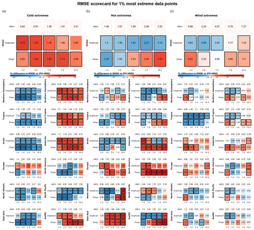
Figure 3 RMSE scorecards for (a) cold, (b) hot, and (c) wind extremes at global and regional scales, computed on (a) the lowest 1 % of data points for 2 m temperature, (b) the highest 1 % of data points for 2 m temperature, and (c) the highest 1 % of data points for 10 m wind speed. Black borders indicate statistically significant differences in performance compared to IFS HRES (at the 5 % level).

A summary scorecard of Figs. 1–3 is provided in Fig. 4, showing which of the three models is best at forecasting cold, hot, and wind speed extremes, as well as 2 m temperature and 10 m wind speed overall. The summary scorecard confirms the patterns observed so far, suggesting that data-driven models are generally superior to IFS HRES in forecasting 10 m wind and 2 m temperature when considering all data points. However, the summary scorecard also shows that the performance of data-driven models degrades relative to IFS HRES when considering extreme quantiles, with IFS HRES being overall superior in forecasting cold extremes in AusNZ and Antarctica and mostly outperforming data-driven models in forecasting hot extremes in Europe, North America, and East Asia. Nevertheless, IFS HRES and data-driven models display comparable performance when forecasting other types of extremes in these regions. Additionally, the summary scorecard highlights the progressive deterioration in the performance of data-driven models compared to IFS HRES for extremes at longer lead times, likely connected to the above-mentioned blurring.

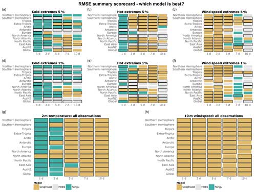
Figure 4 (a–f) Best models in terms of tail RMSE, computed on (a) the lowest 5 % of data points for 2 m temperature, (b) the highest 5 % of data points for 2 m temperature, (c) the highest 5 % of data points for 10 m wind speed, (d) the lowest 1 % of data points for 2 m temperature, (e) the highest 1 % of data points for 2 m temperature, and (f) the highest 1 % of data points for 10 m wind speed. (g–h) Best models in terms of overall RMSE for (g) 2 m temperature and (h) 10 m wind speed. Black borders indicate statistically significantly better performance compared to the other models (at the 5 % level).

Figures 5 and 6 apply criterion 2 (Sect. 2.4) to the comparison between models to evaluate grid-point-level differences in RMSE between IFS HRES and the best data-driven model for each grid point. The data-driven models are better than IFS HRES in terms of overall RMSE in most locations, with one exception concerning 1 d 2 m temperature forecasts, where the performance of the models is highly latitude-dependent. This latitude-dependent pattern can be observed, to a lesser extent, in all other subfigures, where data-driven models consistently perform at their best near the tropics while displaying performance more similar to that of IFS HRES in the extra-tropics. This supports the above-mentioned thesis that the latitude-based weights used by the data-driven models may drive the best performance towards low-latitude areas (see also Figs. 2 and 3).

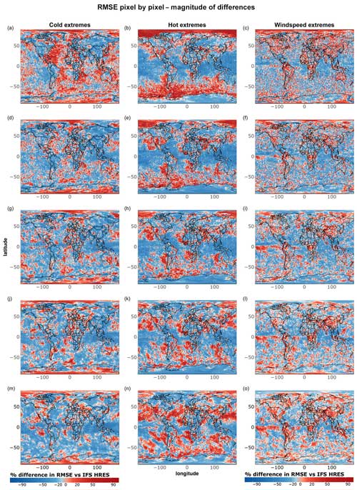
Figure 6 provides complementary information by highlighting the magnitude of the differences between models, independent of their statistical significance. As in previous cases, data-driven models become progressively worse compared to IFS HRES at longer lead times, further supporting the above-mentioned blurring thesis. Moreover, we notice, especially for temperature extremes, a tendency for data-driven models to perform better on the west side of the Pacific and Atlantic oceans and worse on the east side. While this pattern is not as evident as the latitude-dependent and lead-time-dependent performance, it is likely tied to the lack of information on ocean processes and sea-surface temperatures as inputs for the data-driven models. This omission may, for instance, lead to underestimating the effects of underwater currents and upwelling in regions where these processes play an important role in defining local climates (e.g. Abrahams et al., 2021; Jacox et al., 2015; Lemos and Pires, 2004). The lack of information on sea-surface temperatures might also be connected to the subpar performance of data-driven models regarding 10 m wind speed in specific areas within the Intertropical Convergence Zone, such as the Democratic Republic of Congo and northwestern South America (Chiang et al., 2002).

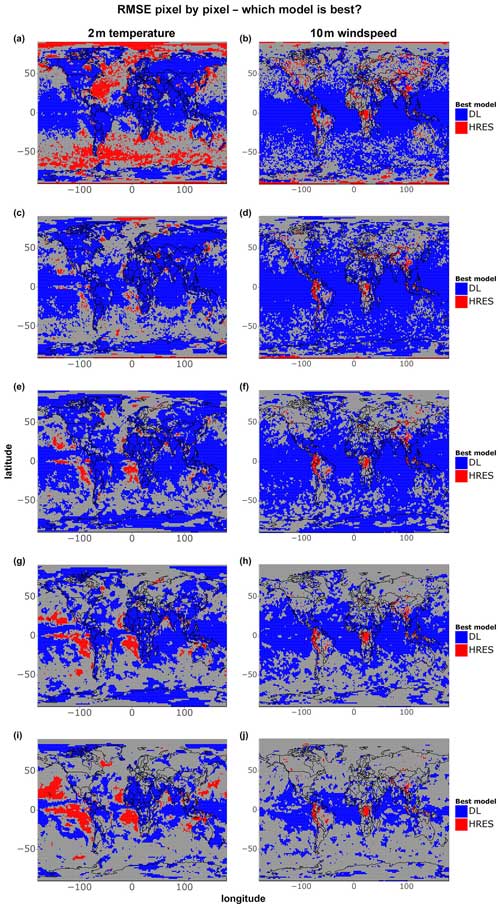
Figure 5 Single-grid-point RMSE comparison for all data points of 2 m temperature and 10 m wind speed. The blue colour indicates that the best data-driven deep learning (DL) model at the corresponding grid point is significantly better than IFS HRES at the 5 % level, while the red colour indicates that IFS HRES is better. The grey colour indicates no statistically significant differences. Shown are (a–b) 1 d forecasts, (c–d) 3 d forecasts, (e–f) 5 d forecasts, (g–h) 7 d forecasts, and (i–j) 10 d forecasts.

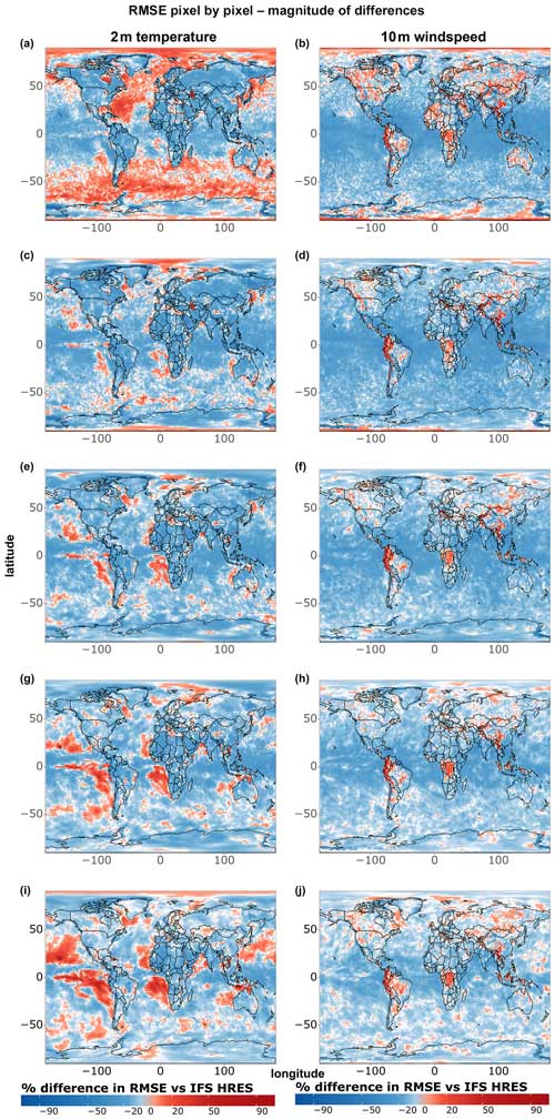
Figure 6 Magnitude of single-grid-point RMSE differences between IFS HRES and the best data-driven model at each grid point for all data points of (a) 2 m temperature and (b) 10 m wind speed. Blue shades indicate better performance demonstrated by the data-driven model, while red shades indicate better performance demonstrated by IFS HRES. Shown are (a–b) 1 d forecasts, (c–d) 3 d forecasts, (e–f) 5 d forecasts, (g–h) 7 d forecasts, and (i–j) 10 d forecasts.

Figures 7 and 8 correspond to Figs. 5 and 6 but focus only on extreme events, namely the 5 % most extreme data points at each grid point during the test period. Fewer differences between models are statistically significant when looking specifically at extremes, likely due to the smaller sample size (n=36) and the fact that IFS HRES and the data-driven models perform more similarly overall. We observe, in particular, only a few significant differences between IFS HRES and the data-driven models regarding wind speed extremes, where the high variance in the magnitude of these wind speed extremes may affect the size of the test statistic and prevent the achievement of statistical significance, even in the presence of large absolute differences in performance.

Despite this, it is still possible to identify some clear patterns. Once more, data-driven models perform best in the tropics overall and worse closer to the poles. This is particularly true for hot extremes, with IFS HRES clearly outperforming data-driven models near the Arctic and in vast ocean areas of the southern extra-tropics. This is largely in line with the findings shown in Figs. 1–4 and is likely ascribable to the same reasons. Additionally, in line with what was previously found in the above-mentioned plots, we find evidence of blurring, especially for cold extremes.

When examining the magnitude of differences between the models (Fig. 8), we observe significant discrepancies in terms of temperature extremes, primarily near the poles and over the oceans. Specifically, for hot extremes, data-driven models tend to perform worse on the eastern sides of ocean basins, consistent with the findings in Fig. 6. Regarding wind speed extremes, the overall poorer performance of data-driven models may again be attributed to the lack of separate training for u- and v-wind components, which can lead to amplified errors for extremes. Additionally, we observe that IFS HRES consistently outperforms data-driven models in many densely populated regions, including parts of the US, China, and northern India. Although these differences are mostly not statistically significant, they nonetheless highlight the need for caution when considering the operationalisation of data-driven models for forecasting wind speed extremes.

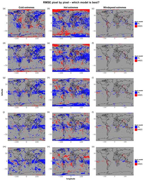
Figure 7 As in Fig. 5 but for cold, hot, and wind speed extremes. The extremes are defined as in Fig. 2 but for individual grid points. Shown are (a–c) 1 d forecasts, (d–f) 3 d forecasts, (g–i) 5 d forecasts, (j–l) 7 d forecasts, and (m–o) 10 d forecasts. The number of data points per grid point is 36.

Figure 8 As in Fig. 6 but for cold, hot, and windy extremes. The extremes are defined as in Fig. 2 but for individual grid points. Shown are (a–c) 1 d forecasts, (d–f) 3 d forecasts, (g–i) 5 d forecasts, (j–l) 7 d forecasts, and (m–o) 10 d forecasts. The number of data points per grid point is 36.

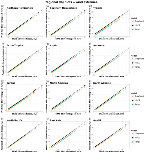
Lastly, we compare the models on the basis of criterion 3 (Sect. 2.4), namely on the ability of different models to reproduce the tail behaviour of ERA5. As in the previous cases, we start by looking at global extremes at multiple lead times (Fig. 9) in order to assess the tail behaviour of the forecasts. Figure 9 suggests that all models appear to be well calibrated in forecasting global cold extremes, while data-driven models tend to underestimate the magnitude of hot and wind speed extremes, especially at longer lead times. This increasing underestimation of extremes at longer lead times by data-driven models is in line with previous findings in this paper related to blurring.

As in previous cases, regional patterns reveal further complexities pertaining to the behaviour of the three models. Figure 10 suggests that all models tend to underestimate cold extremes in the Arctic and North Pacific. Additionally, data-driven models tend to underestimate cold extremes in the Antarctic, and IFS HRES and GraphCast also do so in Europe. The largest underestimation occurs in the Arctic, where the data points corresponding to the coldest temperatures are underestimated by 2–3 K on average across all models. This is in line with previous findings suggesting that data-driven models struggle more with extreme forecasts further away from the tropics. Moreover, we find that the underestimation of cold extremes is, in many cases, more severe for GraphCast than for Pangu-Weather, reinforcing the impression that Pangu-Weather might have a cold bias compared to GraphCast.

This thesis is also supported by Fig. 11, which conversely shows a more severe underestimation of hot extremes for Pangu-Weather and better tail reliability for GraphCast. However, even in this case, IFS HRES displays the best tail reliability overall, while both data-driven models tend to underestimate extremes in several regions, including North America, East Asia, Europe, the tropics, and the North Pacific. AusNZ appears to be the only region where some of the models (IFS HRES and GraphCast) overestimate the average magnitude of the extremes, a finding for which we do not have an immediate explanation. Once more, data-driven models seem to suffer from a more severe lack of calibration in regions further away from the Equator, with the largest underestimations occurring in North America, where the data-driven models underestimate the data points corresponding to the warmest temperatures by around 2 K on average.

Much like it does for temperature extremes, IFS HRES displays almost perfect tail behaviour for wind extremes (Fig. 12), whereas data-driven models tend to slightly underestimate wind speed extremes in all regions. The differences between the models – especially between GraphCast and Pangu-Weather – are, however, smaller overall. The largest difference in tail reliability between GraphCast and Pangu-Weather occurs in the tropics, where, as shown in Figs. 2 and 3, GraphCast appears to outperform Pangu-Weather.

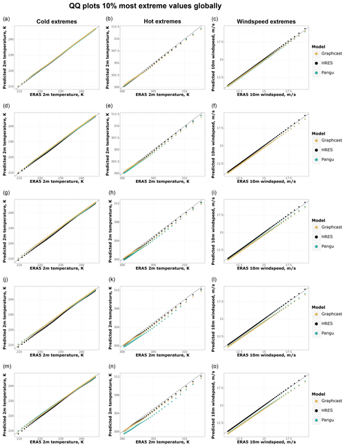
Figure 9 QQ (quantile–quantile) plots of the most extreme 10 % of values for 2 m temperature (cold and hot) and 10 m wind speed forecasts vs. ground truth (ERA5; dashed grey line). Shown are (a–c) 1 d forecasts, (d–f) 3 d forecasts, (g–i) 5 d forecasts, (j–l) 7 d forecasts, and (m–o) 10 d forecasts.

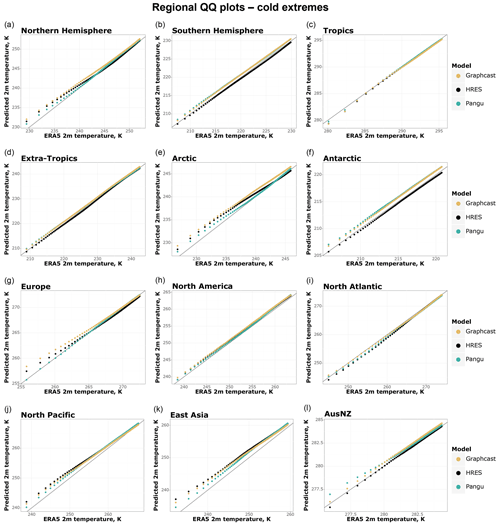
Figure 10 Regional QQ plots of 5 d forecasts for the coldest 10 % of 2 m temperature data points, based on ERA5 2 m temperature data.

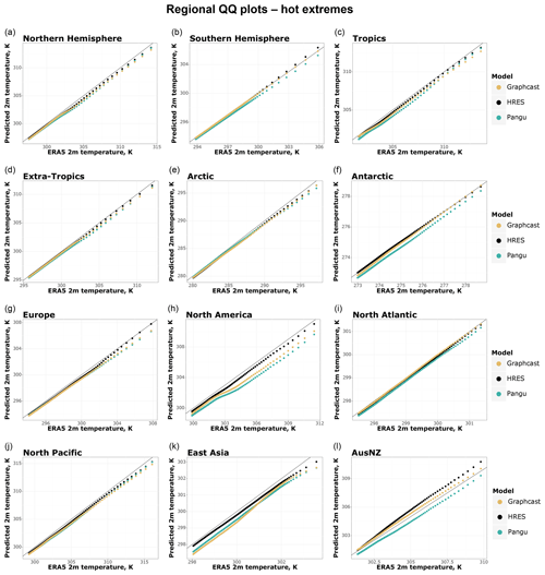
Figure 11 As in Fig. 10 but for the hottest 10 % of 2 m temperature data points, based on ERA5 2 m temperature data.

Figure 12 Regional QQ plots of 5 d forecasts for the windiest 10 % of data points, based on ERA5 10 m wind speed data.

4 Discussion and conclusions

This paper analyses the performance of ECMWF's IFS HRES, GraphCast, and Pangu-Weather in forecasting near-surface temperature and wind speed extremes up to 10 d ahead in a semi-operational setting. Following Watson (2022), the models were evaluated with the help of three criteria (Sect. 2.4), assessing forecast performance (criteria 1 and 2) and the calibration of the forecasts in the tails of the distribution (criterion 3). The results suggest that data-driven models are superior to IFS HRES in forecasting 2 m temperature and 10 m wind speed on average in most regions (Fig. 4), especially in the tropics (Figs. 1 and 5). Notable exceptions include the eastern side of ocean basins for 2 m temperature and selected areas within the Intertropical Convergence Zone for 10 m wind speed. The weaker performance of data-driven models in these areas might be attributed to the lack of information related to ocean dynamics and the omission of sea-surface temperature among their input variables.

In terms of extremes, the performance of the data-driven models is comparable overall with that of IFS HRES, especially with regard to 10 m wind speed (Fig. 7). For temperature extremes, the data-driven models generally outperform IFS HRES in the tropics while exhibiting comparatively weaker performance at higher latitudes. Throughout our evaluation, we observe a pronounced meridional behaviour in the quality of the data-driven forecasts, with a gradual deterioration of performance noted towards higher latitudes. We speculate that this may partly depend on the use of latitude-based weights in the training of the data-driven models, which pushes these models towards the minimisation of large errors closer to the Equator at the expense of performance at higher latitudes.

Our results for 10 m wind speed provide additional arguments for exercising caution in the operationalisation of data-driven models. IFS HRES outperforms the data-driven models in several densely populated land areas, including Europe, the US, and southeastern Asia (Fig. 8). This may partially depend on the stronger spatial heterogeneity of extremes over land regions, where the larger number of variables and the physics-based framework of IFS HRES provide an advantage. The overall weaker performance of the data-driven models for wind speed extremes, compared to temperature extremes, may also depend on the separate training of u- and v-wind components employed by GraphCast and Pangu-Weather.

A more general finding is that the data-driven models perform best in relative terms at shorter lead times, whereas IFS HRES performs best in relative terms at longer lead times (Figs. 1–3). We attribute this behaviour to the phenomenon of blurring, which has been highlighted as a problem faced by deterministic data-driven models in recent studies (Bonavita, 2024; Price et al., 2024). As lead time and uncertainty increase, data-driven models tend to revert to the climatology to minimise large errors. Although this behaviour is common to all weather models, it is more pronounced in deterministic data-driven models than in numerical models. However, probabilistic data-driven models that are currently under development (e.g. Price et al., 2024; Lang et al., 2024; Oskarsson et al., 2024) show promise in addressing this issue. Preliminary results indicate that these models perform better at longer lead times and have a rate of performance decline more similar to that of IFS ENS than to that of deterministic data-driven models (Price et al., 2024).

IFS HRES also appears to be the overall best in terms of tail calibration (Figs. 9–12), even though the differences between IFS HRES and the data-driven models are small for forecasts of global extremes, especially at shorter lead times (Fig. 9). Differences between the two data-driven models are also small overall, with GraphCast oftentimes performing better in the tropics and Pangu-Weather performing better at mid-latitudes (Figs. 4 and 10–12). Additionally, Pangu-Weather appears to be better for cold extremes, while GraphCast performs better for hot extremes.

In the main text, we compare the semi-operational versions of the data-driven models, taking IFS HRES at time 0 as input, with IFS HRES, using ERA5 as the ground truth for all the models. In Appendix D, we shift the focus to comparing reanalysis-based data-driven models with IFS HRES, utilising different ground truths: ERA5 for the data-driven models and IFS HRES at time 0 for the physics-based model. The findings in Appendix D generally support those in the main text (Figs. D1–D7). As noted in the main text, the data-driven models show an improvement over the physics-based model in terms of average skill, with the exception of short-term 2 m temperature forecasts (Figs. D1 and D4), Additionally, the data-driven models are competitive in forecasting extreme events (Figs. D2–D4), with a few exceptions. Specifically, IFS HRES continues to outperform all data-driven models in forecasting cold spells over short lead times, though this might partially be a consequence of the different ground truths used for IFS HRES and the data-driven models. At the grid-point level (Figs. D5–D12), the data-driven models are highly competitive in terms of average skill (Fig. D5), with FuXi standing out due to its remarkable performance in forecasting 2 m temperature at longer lead times. In terms of extremes (Fig. D7), IFS HRES remains superior over land for shorter lead times, but the data-driven models progressively close the gap in the medium range (Fig. D12).

As suggested in the previous literature, some additional challenges need to be addressed before data-driven models can be fully implemented operationally. These challenges include the lack of uncertainty information provided by the deterministic forecasts (Molina et al., 2023; de Burgh-Day and Leeuwenburg, 2023; Scher and Messori, 2021; Clare et al., 2021) and the lack of physical constraints in the forecasts generated by the models (Kashinath et al., 2021; Beucler et al., 2020). Moreover, with the exception of GraphCast, none of the data-driven models that we analysed here can forecast precipitation, which, in extreme cases, is a key meteorological hazard. Finally, further evaluations of extreme forecast behaviour may be necessary. Our analysis is limited to a narrow range of near-surface extremes and, due to current data availability, to extremes that occurred in 2020. This limits our ability to draw conclusions about long-term performance. The short time period considered also exposes our results to sensitivity regarding low-frequency modes of climate variability, which modulate the occurrence of extreme events and may also affect their predictability (Goddard and Gershunov, 2020; Luo and Lau, 2020; Chartrand and Pausata, 2020). We therefore encourage more comprehensive evaluations in the near future as more data become available and deep-learning models are extended to produce forecasts of other relevant variables for weather extremes (e.g. wind gusts and precipitation).

We also note that all forecast evaluation metrics, including those used here, suffer from limitations: for criteria 1 and 2, the RMSE is also the objective function of the machine learning (ML) models, which means that evaluating against RMSE is not a fully independent benchmark. Additionally, criteria 1 and 2 are not proper or consistent scores, meaning that it would be possible to design a data-driven model that optimises for tail RMSE that outperforms all other models while ignoring other aspects of performance (Taggart, 2022; Lerch et al., 2017). We note, however, that this limitation applies to most metrics of tail performance used by deterministic models found in the previous literature, including the widely popular precision–recall curves. Similarly, criterion 3 is only a measure of tail calibration, which can be maximised using post-processing schemes that place greater emphasis on tail behaviour than on the rest of the distribution. For this reason, inference based on any of these measures alone is not meaningful, and any tail comparison between models should be integrated with comparisons for the entire distribution of the variables, such as those presented in Figs. 1 and 5, and with more qualitative measures of performance. Additionally, as highlighted by Watson (2022), raw measures of performance and QQ (quantile–quantile) plots should also be complemented by a careful study of weather charts from case studies. In particular, we emphasise that better performance in just one of the three criteria used in this paper should not be interpreted in isolation as evidence of the overall superiority of one model over the others.

To strengthen our results, we include, in Appendix B and C, two additional metrics of tail performance that cannot be hedged by data-driven models in the same way that criteria 1 and 2 can. The results there are mostly in line with what is shown in the main text, suggesting that none of the data-driven models included in this paper have hedged the tail RMSE metrics included in our main analysis. However, the metrics presented in Appendix B and C suffer from a fundamental limitation: they select either part of or all of their extreme samples based on forecasts rather than on an independent ground truth. This leads to a progressive deterioration in the selection criteria for extremes with lead time, thus introducing a fundamental issue regarding the validity of the sample. Moreover, the fact that the sample becomes increasingly less representative of the ground truth extremes at longer lead times tends to favour data-driven models, which, as shown by WeatherBench 2 (Rasp et al., 2024) and in this paper, are mostly superior in terms of standard metrics based on the overall distribution of near-surface variables.

We conclude that data-driven models can already compete with physics-based models in the forecasting of near-surface temperature and wind extremes. However, the performance of data-driven models varies by region, type of extreme event, and forecast lead time. The main challenges holding data-driven models back appear to be blurring, poor performance at high latitudes, and a lack of some key input variables. As solutions to blurring appear to be in sight, we argue that more attention should be given to loss functions and input variables. We therefore encourage more studies in this direction, particularly to investigate whether removing latitude-based weights from the training routine might lead to better performance with regard to extremes at higher latitudes.

As of now, we can already envisage a hybrid approach using both physics- and data-driven models to forecast extremes, with physics-based models supplemented by data-driven models in areas where data-driven models have been shown to be superior in terms of tail performance, such as in the tropics. This hybrid usage could take the form of a fully hybrid model, such as the recent neural general circulation model NeuralGCM (Kochkov et al., 2024), or even the form of simple post-processing schemes based on weighted averages of physics-based and data-driven forecasts.

Appendix A: Pixel-by-pixel comparisons including individual data-driven models

This section includes figures complementary to Figs. 5–8, displaying which of the models performs best at each pixel (Figs. A1 and A2) and the magnitude of corresponding differences (Figs. A3 and A4).

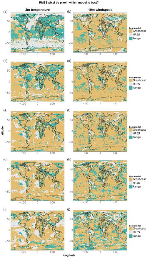
Figure A1 Single-grid-point RMSE comparison for all data points of 2 m temperature and 10 m wind speed. Shown are (a–b) 1 d forecasts, (c–d) 3 d forecasts, (e–f) 5 d forecasts, (g–h) 7 d forecasts, and (i–j) 10 d forecasts.

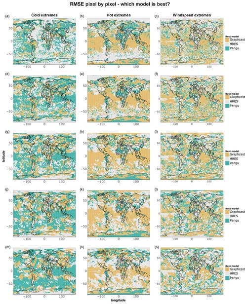
Figure A2 Single-grid-point RMSE comparison for cold, hot, and wind speed extremes. Shown are (a–c) 1 d forecasts, (d–f) 3 d forecasts, (g–i) 5 d forecasts, (j–l) 7 d forecasts, and (m–o) 10 d forecasts.

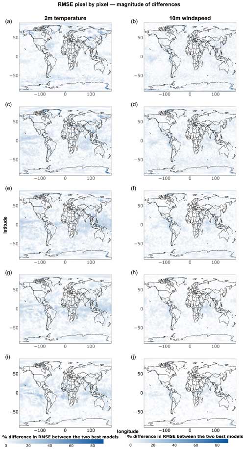
Figure A3 Magnitude of single-grid-point RMSE differences between the two best models at each grid point for all data points of 2 m temperature and 10 m wind speed. Shown are (a–c) 1 d forecasts, (d–f) 3 d forecasts, (g–i) 5 d forecasts, (j–l) 7 d forecasts, and (m–o) 10 d forecasts.

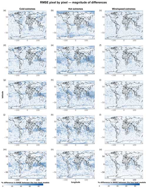
Figure A4 As in Fig. A3 but for cold, hot, and wind speed extremes.

Appendix B: Comparison of consistent scores emphasising tail performance

We report here the results of additional evaluations of tail performance based on the Taggart (2022) mean-squared-error (MSE) decomposition (Eqs. 1 and 2 in Taggart, 2022), where we emphasise performance in the tails by means of a rectangular partition, with the cutoff values determined by extreme quantiles of all ground truth (ERA5) data points for the given region. In Figs. B1 and B2, we only include the scores for the part of the decomposition emphasising tail performance (S1 for cold extremes and S2 for hot and wind speed extremes). Since S is the MSE in this case, it can be easily computed by squaring the values reported in Fig. 1. Since $S=S\mathrm{1}+S\mathrm{2}$, the remaining part of the decomposition not displayed here can be obtained by subtracting the results reported below from the MSE (S).

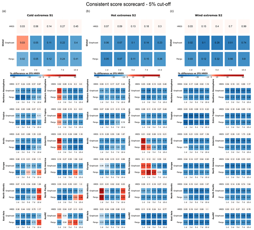
Figure B1 Scorecards for (a) cold, (b) hot, and (c) windy extremes based on rectangular partitions, with the (a) 5th and (b–c) 95th quantiles of all test data points in the given region presented as cutoff values. Blue shades indicate performance better than that of IFS HRES, while red shades indicate worse performance.

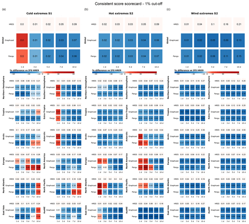
Figure B2 Scorecards for (a) cold, (b) hot, and (c) windy extremes based on rectangular partitions, with the (a) 1st and (b–c) 99th quantiles of all test data points in the given region presented as cutoff values. Blue shades indicate performance better than that of IFS HRES, while red shades indicate worse performance.

Appendix C: Comparison of extremes selected based on the IFS HRES forecasts

We report here the results of additional evaluations of tail performance, where we select the extremes based on the IFS HRES forecast and respective quantile thresholds instead of the ground truth, i.e. the ERA5 reanalysis. This approach has the advantage of preventing the risk of hedging caused by data-driven models, but it has the fundamental disadvantage of introducing validity issues into the extreme sample since the quality of the forecasts – and, therefore, the quality of the selection of the extremes – decreases with lead time.

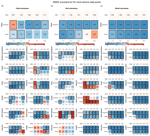
Figure C1 RMSE scorecards for (a) cold, (b) hot, and (c) wind extremes at global and regional scales, computed on (a) the lowest 5 % of data points for 2 m temperature, (b) the highest 5 % of data points for 2 m temperature, and (c) the highest 5 % of data points for 10 m wind speed, selected on the basis of the IFS HRES forecast. Black borders indicate statistically significant differences in performance compared to IFS HRES (at the 5 % level).

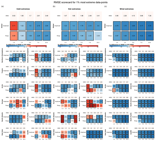
Figure C2 RMSE scorecards for (a) cold, (b) hot, and (b) wind extremes at global and regional scales, computed on (a) the lowest 1 % of data points for 2 m temperature, (b) the highest 1 % of data points for 2 m temperature, and (c) the highest 1 % of data points for 10 m wind speed, selected on the basis of the IFS HRES forecast. Black borders indicate statistically significant differences in performance compared to IFS HRES (at the 5 % level).

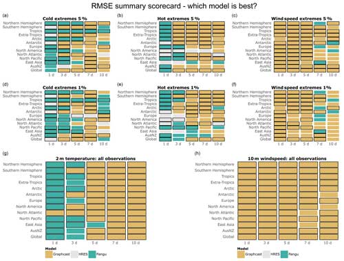
Figure C3 (a–f) Best models in terms of tail RMSE, computed on (a) the lowest 5 % of data points for 2 m temperature, (b) the highest 5 % of data points for 2 m temperature, (c) the highest 5 % of data points for 10 m wind speed, (d) the lowest 1 % of data points for 2 m temperature, (e) the highest 1 % of data points for 2 m temperature, and (f) the highest 1 % of data points for 10 m wind speed, selected on the basis of the IFS HRES forecast. (g–h) Best models in terms of overall RMSE for (g) 2 m temperature and (h) 10 m wind speed. Black borders indicate statistically significantly better performance compared to the other models (at the 5 % significance level).

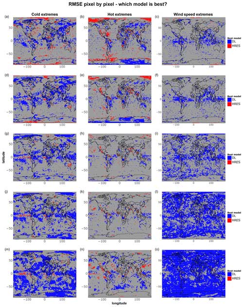
Figure C4 As in Fig. 7 but with the extremes selected on the basis of the IFS HRES forecast instead of the ground truth (ERA5).

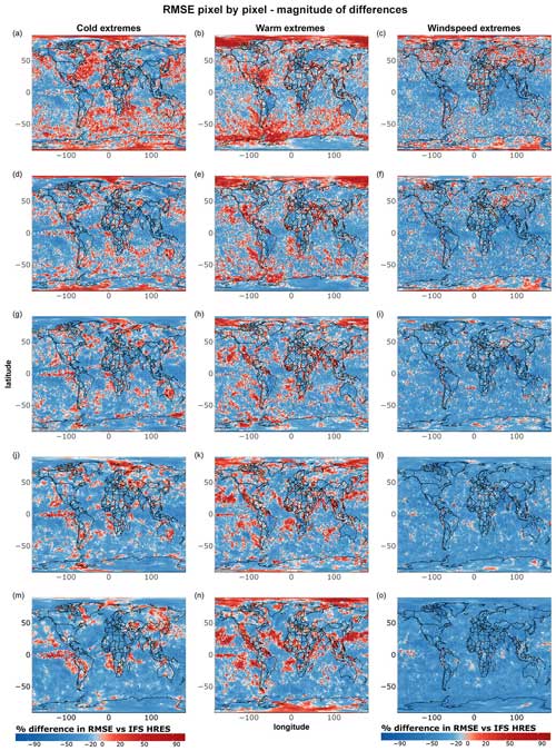
Figure C5 As in Fig. 8 but with the extremes selected on the basis of the IFS HRES forecast instead of the ground truth (ERA5).

Appendix D: Comparison of reanalysis-based data-driven models

Here, we provide global and regional scorecards and grid-point-level comparisons for data-driven models using ERA5 reanalysis data as input. Following WeatherBench 2 (Rasp et al., 2024), we attempt to make the comparison between reanalysis-based data-driven models and IFS HRES as fair as possible by using IFS HRES at t=0, instead of ERA5, as the ground truth for IFS HRES.

In this comparison, we also include FuXi (Chen et al., 2023b), a recent data-driven model building upon the work of Bi et al. (2023). Forecasts generated by FuXi are currently available only on WeatherBench 2 for the reanalysis-based version of the model (Rasp et al., 2024), which is why we include FuXi here but not in the comparisons presented in the main text. FuXi is trained on ERA5 reanalysis data from 1979 to 2017 and uses a vision transformer architecture (Dosovitskiy et al., 2020). FuXi's main innovation compared to previous models is its cascading optimisation approach, through which different sub-models are developed for different forecasting ranges, with the purpose of improving medium–long-range forecasts (Chen et al., 2023b).

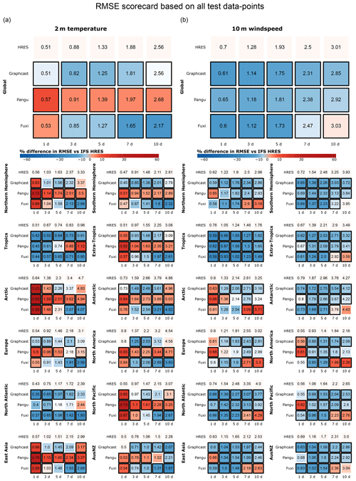
Figure D1 As in Fig. 1 but using ERA5 as the ground truth for the data-driven forecasts and IFS HRES at time 0 as the ground truth for the IFS HRES forecasts.

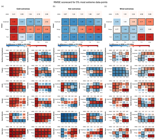
Figure D2 As in Fig. 2 but using ERA5 as the ground truth for the data-driven forecasts and IFS HRES at time 0 as the ground truth for the IFS HRES forecasts.

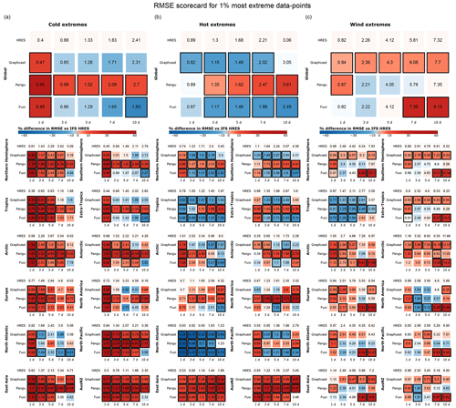
Figure D3 As in Fig. 3 but using ERA5 as the ground truth for the data-driven forecasts and IFS HRES at time 0 as the ground truth for the IFS HRES forecasts.

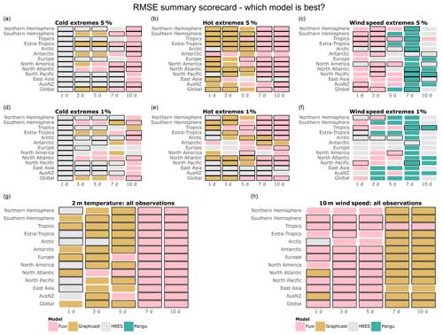
Figure D4 As in Fig. 4 but using ERA5 as the ground truth for the data-driven forecasts and IFS HRES at time 0 as the ground truth for the IFS HRES forecasts.

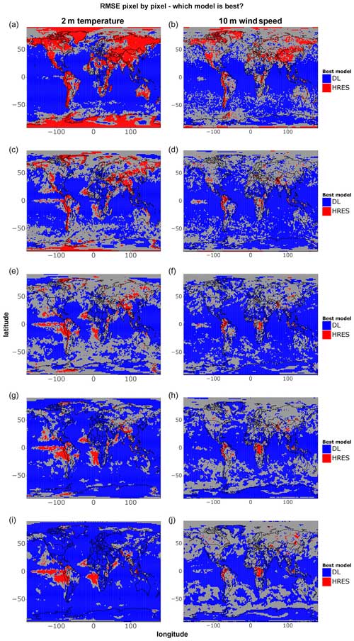
Figure D5 As in Fig. 5 but including FuXi among the possible data-driven models and using ERA5 as the ground truth for the data-driven forecasts and IFS HRES at time 0 as the ground truth for the IFS HRES forecasts.

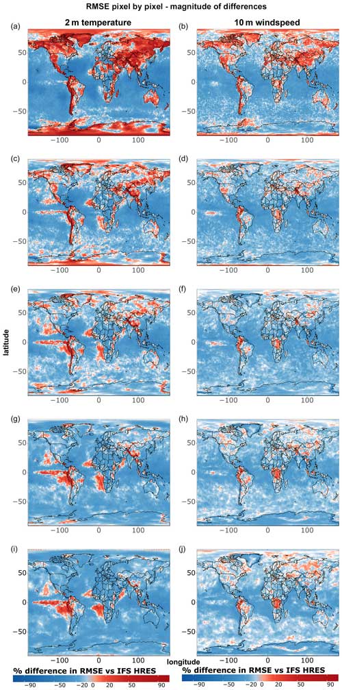
Figure D6 As in Fig. 6 but including FuXi among the possible data-driven models and using ERA5 as the ground truth for the data-driven forecasts and IFS HRES at time 0 as the ground truth for the IFS HRES forecasts.

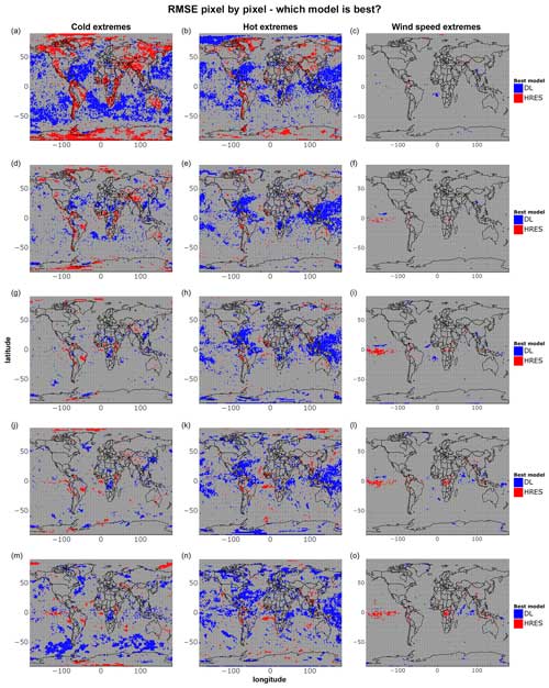
Figure D7 As in Fig. 7 but including FuXi among the possible data-driven models and using ERA5 as the ground truth for the data-driven forecasts and IFS HRES at time 0 as the ground truth for the IFS HRES forecasts.

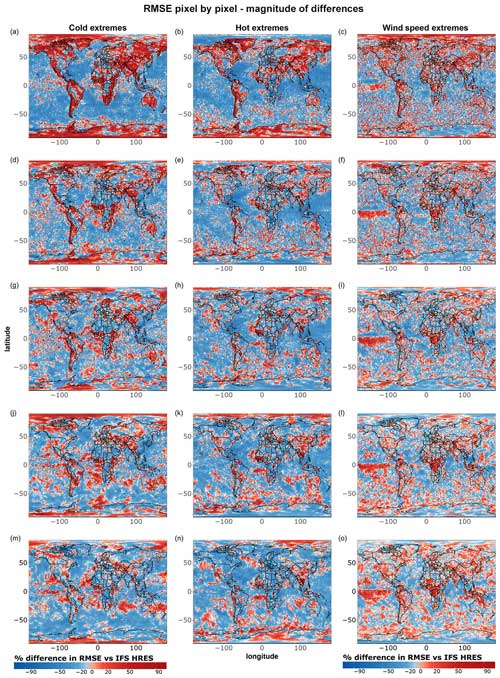
Figure D8 As in Fig. 8 but including FuXi among the possible data-driven models and using ERA5 as the ground truth for the data-driven forecasts and IFS HRES at time 0 as the ground truth for the IFS HRES forecasts.

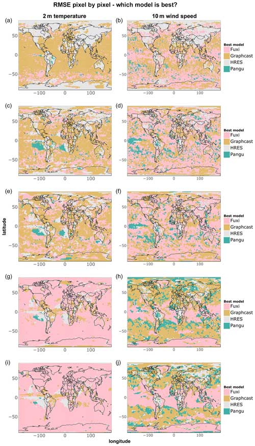
Figure D9 As in Fig. A1 but using ERA5 as the ground truth for the data-driven forecasts and IFS HRES at time 0 as the ground truth for the IFS HRES forecasts.

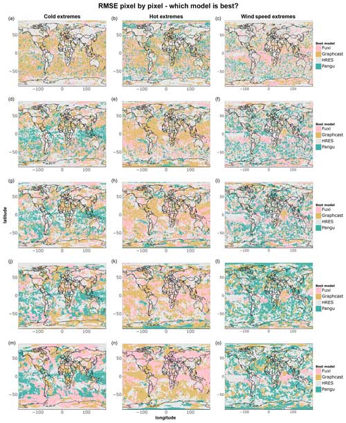
Figure D10 As in Fig. A2 but using ERA5 as the ground truth for the data-driven forecasts and IFS HRES at time 0 as the ground truth for the IFS HRES forecasts.

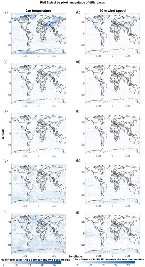
Figure D11 As in Fig. A3 but using ERA5 as the ground truth for the data-driven forecasts and IFS HRES at time 0 as the ground truth for the IFS HRES forecasts.

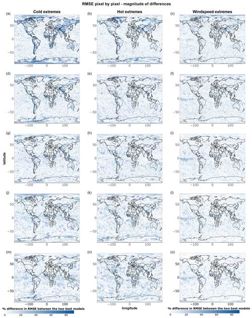
Figure D12 As in Fig. A4 but using ERA5 as the ground truth for the data-driven forecasts and IFS HRES at time 0 as the ground truth for the IFS HRES forecasts.