PPCon 1.0: Biogeochemical-Argo profile prediction with 1D convolutional networks

Effective observation of the ocean is vital for studying and assessing the state and evolution of the marine ecosystem and for evaluating the impact of human activities. However, obtaining comprehensive oceanic measurements across temporal and spatial scales and for different biogeochemical variables remains challenging. Autonomous oceanographic instruments, such as Biogeochemical (BGC)-Argo profiling floats, have helped expand our ability to obtain subsurface and deep-ocean measurements, but measuring biogeochemical variables, such as nutrient concentration, still remains more demanding and expensive than measuring physical variables. Therefore, developing methods to estimate marine biogeochemical variables from high-frequency measurements is very much needed. Current neural network (NN) models developed for this task are based on a multilayer perceptron (MLP) architecture, trained over point-wise pairs of input–output features. Although MLPs can produce smooth outputs if the inputs change smoothly, convolutional neural networks (CNNs) are inherently designed to handle profile data effectively. In this study, we present a novel one-dimensional (1D) CNN model to predict profiles leveraging the typical shape of vertical profiles of a variable as a prior constraint during training. In particular, the Predict Profiles Convolutional (PPCon) model predicts nitrate, chlorophyll, and backscattering (bbp700) starting from the date and geolocation and from temperature, salinity, and oxygen profiles. Its effectiveness is demonstrated using a robust BGC-Argo dataset collected in the Mediterranean Sea for training and validation. Results, which include quantitative metrics and visual representations, prove the capability of PPCon to produce smooth and accurate profile predictions improving upon previous MLP applications.

1 Introduction

Observation of the ocean is crucial for studying the state and evolution of the marine ecosystem and for assessing the impact of human activities (Campbell et al., 2016; Euzen et al., 2017). Access to reliable and extensive oceanic measurements remains restricted due to the challenges of collecting comprehensive observations on multiple temporal and spatial scales and of variability in the availability of observations across different biogeochemical variables (Munk, 2000).

The introduction of autonomous oceanographic instruments, such as Biogeochemical (BGC)-Argo floats, has notably expanded our ability to obtain subsurface and deep-ocean measurements (Miloslavich et al., 2019). BGC‐Argo floats are autonomous profiling platforms that incorporate physical and biogeochemical sensors, enabling us to collect time series of vertical profiles across various sea conditions and throughout the complete annual cycle (d'Ortenzio et al., 2014; Mignot et al., 2014). Over the past decade, there has been a steady rise in the number of biogeochemical profiles acquired using these platforms (Johnson et al., 2013; Johnson and Claustre, 2016). These instruments are essential to advancing our knowledge of the biogeochemical state of the ocean, as one of their principal use cases is the assimilation into ocean biogeochemical models (Mignot et al., 2019; D'ortenzio et al., 2020). This assimilation process is particularly promising for variables such as oxygen, nitrate, and chlorophyll concentrations, as they serve as core state variables in most ocean biogeochemical models (Teruzzi et al., 2021; Cossarini et al., 2019).

However, the measurement of biogeochemical variables, such as nutrient concentration and carbonate system variables (e.g., nitrate, chlorophyll, and pH), remains more demanding and expensive compared to physical variables (e.g., temperature and salinity) and oxygen. In fact, among the BGC sensors, oxygen is the most commonly measured variable: there have been approximately 250 000 oxygen profiles collected worldwide, which is twice the number of profiles for chlorophyll and more than 4 times the number of profiles for nitrate and bbp700 (https://biogeochemical-argo.org, last access: 18 June 2024). Thus, developing methods to estimate low-frequency marine biogeochemical variables from high-frequency measurements is essential to maximize the potential of observing systems such as the Argo program. Major efforts have been devoted to the improvement of the long-term reliability and accuracy of autonomous measurements in recent years (Sauzède et al., 2017).

Artificial neural networks (ANNs) are computational models that are inspired by the structure and function of the human brain, and they have become a widely used approach for solving complex problems in a variety of fields, from computer vision and natural language processing to finance and engineering (Krogh, 2008). ANNs have also emerged as a powerful tool for modeling complex non-linear relationships in the oceanographic field, where their use has seen a significant increase in recent years (Ahmad, 2019). The use of these models has found applications in a wide range of areas, such as oceanic climate prediction and forecasting (Mori et al., 2017), species identification (Goodwin et al., 2014), coastal morphological and morphodynamic modeling (Goldstein et al., 2019), ocean current prediction (Bolton and Zanna, 2019), interpolation and gap filling for remote-sensing observation (Sammartino et al., 2020), and the integration of observation data into biogeochemical models (Pietropolli et al., 2022). These examples demonstrate the broad utility of ANNs in advancing our understanding of the ocean and its processes.

Existing ANN-based techniques to infer low-sampled variables starting from high-sampled ones are based on multilayer perceptron (MLP) architecture, a type of feed-forward neural network (NN) that processes input data through interconnected layers of nodes, or neurons, with each neuron in a layer receiving inputs from all the neurons in the previous layer (Taud and Mas, 2018). The initial model designed for this task was proposed by Sauzède et al. (2017), where a deterministic MLP network, named CANYON, was trained on a global ocean dataset to estimate biogeochemically relevant variables from concurrent in situ samples of temperature, salinity, pressure, and oxygen and their latitude, longitude, depth, and date. Later, an improved version, called CANYON-B, was introduced by Bittig et al. (2018). In this approach, a Bayesian framework was utilized, and experimental findings demonstrated that this method resulted in a more robust output. This methodology was subsequently limited to the Mediterranean Sea, resulting in the development of CANYON-MED by Fourrier et al. (2020), and empirical results validated the effectiveness of restricting the model to a smaller region. The latest advancement in this field is presented in Pietropolli et al. (2023a), wherein the authors enhance the performance related to Mediterranean Sea predictions by leveraging a more extensive training dataset and implementing a two-step quality-check procedure to improve its quality.

Despite their widespread use, applications based on MLPs currently lack awareness of the typical shape of the biogeochemical variable profiles they aim to infer. When these methods are used to predict profiles from Argo float measurements, they may generate irregularities in the reconstruction, possibly because they use point-wise data as input and output.

To solve this problem effectively, our idea consists of working directly with an architecture that infers the complete vertical profile. This approach takes advantage of architectures like the convolutional neural network (CNN) that operate on vector inputs instead of individual points. CNNs are recognized as one of the most impressive forms of ANNs, especially for their effectiveness in tackling complex pattern recognition problems (O'Shea and Nash, 2015; Gu et al., 2018). While CNNs are well known for their success in image classification tasks, they can also be used for other tasks, such as speech recognition (Shan et al., 2018), natural language processing (Collobert et al., 2011), and even drug discovery (Goh et al., 2017).

In this study, we evaluate the effectiveness of a one-dimensional (1D) CNN model (Kiranyaz et al., 2021) for predicting nutrient vertical profiles from input data, such as sampling time, geolocation, and profiles of temperature, salinity, and oxygen, using Argo float measurements as the training dataset. This approach, called PPCon (Predict Profiles Convolutional), is applied to generate synthetic profiles of nitrate, chlorophyll, and backscattering (bbp700). Thanks to the intrinsic spatially aware nature of its CNN architecture, PPCon can leverage the typical shape of vertical profiles of a variable as a prior constraint during training. The PPCon approach is tested with a robust Argo dataset collected in the Mediterranean Sea. The Mediterranean Sea, a semi-enclosed marginal sea, presents a substantially high density of BGC-Argo profiles thanks to dedicated programs such as ARGO-Italy and the French NAOS initiative (D'ortenzio et al., 2020). This particularly fortunate situation has already made the Mediterranean a successful case study for the development of biogeochemical modeling approaches based on BGC-Argo. For example, BGC-Argo is being integrated into the biogeochemical prediction model of the Mediterranean component of the Copernicus Marine Service (Cossarini et al., 2019; Teruzzi et al., 2021; Coppini et al., 2023).

This paper is organized as follows: Sect. 2 presents the dataset utilized for training the deep learning (DL) architecture, including its key characteristics. Section 3 provides a detailed overview of the PPCon approach, encompassing the architecture, the preprocessing techniques applied to input data, and the specialized loss function employed for network training. In Sect. 4, we outline the specific experimental settings employed to enable complete reproducibility of the PPCon architecture. Section 5 presents a summary of the key results obtained during the experimental campaign we conducted to validate our proposed techniques, and Sect. 6 discusses the results obtained. Finally, Sect. 7 presents the conclusions drawn from our work and directions for future research.

2 Dataset: the Argo GDACs

The data used to train and test the architecture discussed in this paper come from the BGC-Argo program (Bittig et al., 2019), specifically the Argo float also collecting biogeochemical variables (BGC-Argo float).

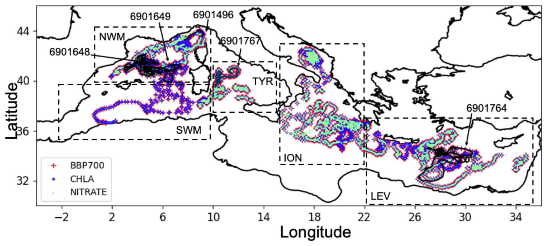
Figure 1 Positions of BGC-Argo float profiles for bbp700 (red), chlorophyll (blue), and nitrate (green) that also have oxygen data. Positions of the four BGC-Argo float profiles used for the external validation (black and numeric labels). Geographical limits of sub-regions (dashed boxes): northwestern Mediterranean Sea (NWM), southwestern Mediterranean Sea (SWM), Tyrrhenian Sea (TYR), Ionian and southern Adriatic Sea (ION), and Levantine Sea (LEV).

Our investigation used BGC-Argo S-profile data for the Mediterranean Sea downloaded from the Coriolis Argo GDAC (Argo, 2000; last visit in August 2022), and the analysis considered only delayed-mode (DM) and adjusted real-time (RT) data for the period from 1 July 2013 to 31 December 2020, ensuring a larger number of DM data. A quality-check procedure was applied as described in Amadio et al. (2023). The Python package “bit.sea” (/float), available via Zenodo (Bolzon et al., 2023), was used for this purpose. The quality-checked BGC-Argo dataset used as input for the present application can also be accessed via Zenodo (Amadio et al., 2023).

Specifically, the dataset was checked by retrieving only complete profiles with quality flags 1 (good data), 2 (probably good data), 5 (value changed), and 8 (interpolated) for temperature, salinity, nitrate, oxygen, and chlorophyll. Additionally, three specific quality-check steps were applied for bbp700 based on the study by Dall'Olmo et al. (2022): a missing-data test (for profiles with a substantial number of missing data), a high-deep-value test (for profiles with unusually high bbp700 value at depth), and a negative-bbp test (for profiles with negative bbp700 values). If the vertical resolution of the profiles was more than 2 m, the data were averaged to a 2 m resolution. A moving weighted average was then applied to smooth out eventual small fluctuations, using the two upper and two lower neighboring points, with a Gaussian function of the distance to the central point to determine the weights. The spatial distribution of the floats after the quality check is shown in Fig. 1.

3 PPCon: Predict Profiles Convolutional neural network

This section introduces the PPCon architecture, which is primarily a 1D CNN with additional MLPs employed to transform point-wise data into a vectorial shape – necessary for training the convolutional component. The input for PPCon includes sampling data, geolocation, temperature, salinity, and oxygen, while the PPCon output comprises vertical profiles for nitrate, chlorophyll, and BBP. Despite using the same architecture, a separate model is trained for each output variable, and different hyperparameters (number of epochs, weights of the loss function, and so on) are set for each of them. This separate tuning is necessary due to some intrinsic differences, such as the numerosity of the training set and the variable ranges. The hyperparameters are tuned manually by comparing performance on the test set composed of unseen data, based on a fitness metric to be introduced later. A specific loss function is designed to promote good performances, good generalization capabilities, and smooth predictions.

3.1 Input preprocessing

The data considered for feeding the DL architecture comprise a collection of measurements, where each input–output pair consists of the information collected by a single float profile. The inputs consist of two distinct categories of data, namely point-wise and vectorial. Point-wise data encompass temporal and geospatial parameters, such as the sample date (specifically year and day) and geographic coordinates (latitude and longitude), while vectorial data encapsulate profiles of temperature, salinity, and oxygen, as recorded by the float instruments. Given that the 1D CNN architecture operates only on vectorial input data, a coherent transformation of point-wise features into vectorial ones is required.

In this regard, we leverage an MLP architecture that accepts point-wise input and transforms it into vectorial form. MLPs are employed to enable the NN to automatically learn how to weigh the importance of such point-wise input features differently in correspondence to different levels of depth. A separate MLP is trained for each of the four point-wise inputs. The MLP architectures have the same number of layers and neurons contained in these layers (Table 1), since there are no a priori reasons to make them different.

Table 1 The MLP component of the PPCon model illustrated in diagram form. All four MLPs used in the PPCon architecture share the same architecture.

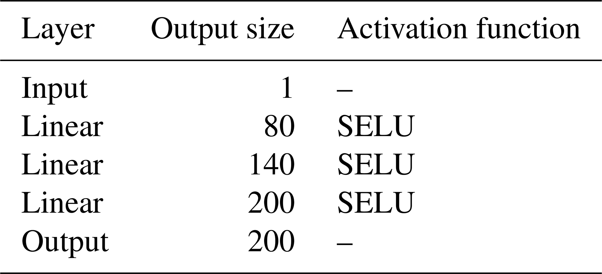
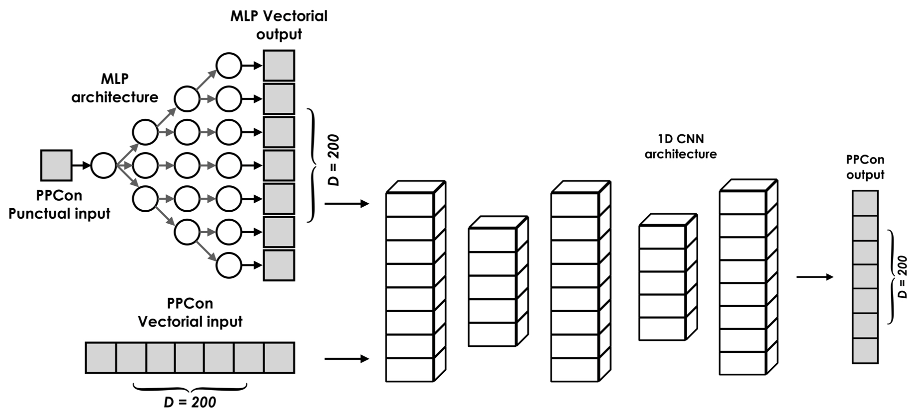
Figure 2 Illustration of the principal architectural components of the PPCon model: (i) MLP network to transform the point-wise inputs (day, year, latitude, and longitude) into vectorial form, (ii) vectorial inputs (output of the MLP and profiles of temperature, salinity, and oxygen), (iii) structure of the encoder–decoder of a 1D CNN architecture, and (iv) output vector representing the vertical profile of one of the target variables (nitrate, chlorophyll, or backscattering).

During training, the weights of the MLP are optimized along with the weights of the 1D CNN architecture. Since the MLP operates as a non-linear function, this training approach enables the creation of a mapping between a point-wise input and its vectorial equivalent. This enables PPCon to effectively exploit point-wise information and achieve optimal learning outcomes. The output vectors generated by the MLP are concatenated with the remaining vectorial input, yielding a seven-channel tensor that serves the input of the PPCon architecture.

Thus, to sum up, the input to the PPCon architecture consists of four point-wise inputs (latitude, longitude, day, and year), which are transformed into a vectorial input using an MLP architecture. In addition, for the training, the architecture uses three 1×200 input vectors representing the profiles of temperature, salinity, and oxygen.

3.2 PPCon architecture

The convolutional component of the PPCon architecture, summarized in Table 2, is a DL model comprising multiple 1D convolutional and deconvolutional layers.

Table 2 The convolutional component of the PPCon model is illustrated in diagram form. The key attributes of the NN are outlined, encompassing parameters, output size (represented as [number of channels, input length]), and any additional layers. More specifically, “BN” denotes the batch normalization layer, “SELU” represents the non-linear selu() activation layer, and “Dropout” indicates the presence of a dropout layer along with the corresponding dropout rate.

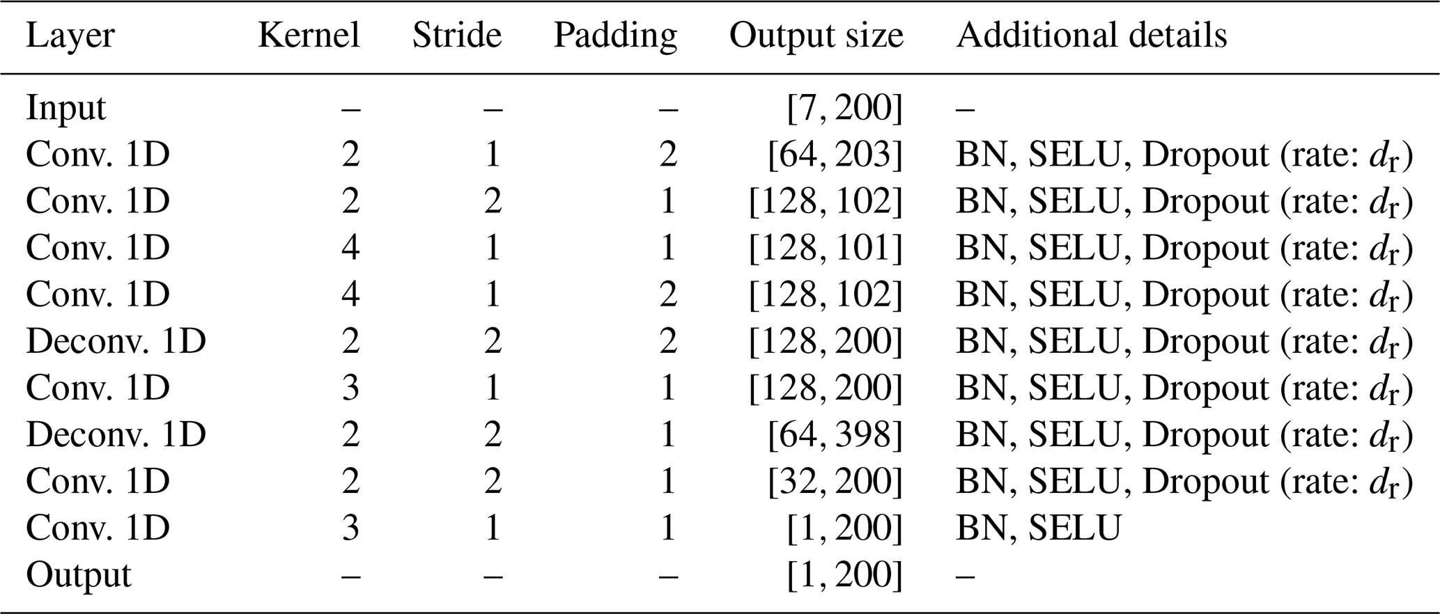
The input tensor has a one-dimensional shape, with a total of seven channels, one for each of the three variables to reconstruct, i.e., nitrate, chlorophyll, and bbp700.

The architecture includes a total of nine layers, each of which applies a set of filters to the input tensor. These filters are designed to detect specific features or patterns, with the number and size of the filter kernels specified by the parameters of each layer. To enable effective feature extraction across different scales, various stride parameters are employed to specify the step size at which the filters are applied to the input tensor. To ensure that the output tensor has the same shape as the input tensor, padding parameters are incorporated, adding zero padding to the borders of the input tensor. The output tensor is then normalized through a batch normalization (Santurkar et al., 2018) layer after each convolutional layer. The normalization process ensures that the output tensor has a mean of zero and a unit variance, thereby minimizing the effect of covariate shifts and enhancing the stability of the training process. Following normalization, the output tensor is passed through a scaled exponential linear unit (SELU) activation function (Rasamoelina et al., 2020), which is defined as

$$\begin{array}{}\text{(1)}& f\left(x\right)=\left\{\begin{array}{ll}\mathit{\lambda }x& \text{if }x\ge \mathrm{0}\\ \mathit{\lambda }\mathit{\alpha }\left(e^x\right)& \text{if }x<\mathrm{0},\end{array}\right.\end{array}$$

where λ≈1.0507 and α≈1.6732. SELU was selected as an activation function, as it induces self-normalization properties. Dropout layers (Baldi and Sadowski, 2013) are also incorporated to prevent overfitting during training, promoting robust generalization and enhancing the NN's ability to learn diverse features from the input data. These layers randomly drop out some of the network neurons, with the specific probability of dropout (d_r) specified for each layer in the architecture's hyperparameters.

The final convolutional layer produces a one-channel output tensor, which represents the final prediction of the model.

3.3 Loss function

The choice and design of a loss function is a crucial step in the development of DL models, as it determines the objective to be optimized during training and can have a significant impact on the model's ability to generalize to new data. Besides the ability to skillfully reproduce output variable profiles, we want the PPCon architecture to mitigate overfitting and produce a smooth prediction curve.

To fulfill these objectives, we define a loss function comprising three components: firstly, the root-mean-square error (RMSE) between the target output and the PPCon architecture's prediction, to assess prediction quality. Secondly, to mitigate overfitting phenomena, a regularization term known as λ regularization is employed, which penalizes complex curves in proportion to the square of the model's weights (Zou and Hastie, 2005). By promoting smaller weight values, this technique encourages the generation of more general predictions. The severity of this penalty is determined by a multiplicative factor λ, which is a hyperparameter of the model. The final component of the loss function is incorporated to promote the generation of a smoother output curve. This term, controlled by a hyperparameter α_s, serves as a regularization technique that penalizes sharp variations in the output. The final loss formula is as follows:

$$\begin{array}{}\text{(2)}& \mathcal{L}(y,\widehat{y})=\sum _{i=\mathrm{1}}^n(y_i-{\widehat{y}}_i{)}^{\mathrm{2}}+\mathit{\lambda }\sum _{i=\mathrm{1}}^N|{\mathit{\theta }}_i{|}^{\mathrm{2}}+{\mathit{\alpha }}_{\mathrm{s}}\sum _{i=\mathrm{1}}^{n-\mathrm{1}}({\widehat{y}}_{i+\mathrm{1}}-{\widehat{y}}_i{)}^{\mathrm{2}},\end{array}$$

where y represents the target value, $\widehat{y}$ is the output of the PPCon model, n is the length of both y and $\widehat{y}$, and N is the total number of weights of the DL architecture.

4 Experimental study

This section presents the experimental settings for the PPCon architecture, which are defined for each predicted variable under consideration. The complete code for the reproducibility of the results presented in this paper is available at https://doi.org/10.5281/zenodo.8369573 (Pietropolli et al., 2023b).

Moreover, a Python library is provided, which can be installed via pip install ppcon, and the corresponding code and documentation are available at https://github.com/gpietrop/ppcon (last access: 15 September 2024). The library allows users to train the PPCon architecture and use the pretrained architecture described in this paper to predict new profiles, and it includes functions to reproduce all the plots presented in this paper.

4.1 Training

We divided the dataset into three subsets: training, testing, and validation. The training set was used for model training and parameter optimization. The testing set was utilized to evaluate the model's performance on unseen data and assess its generalization ability. Finally, the validation set was employed for hyperparameter tuning and model selection. The dataset was randomly partitioned, ensuring that each subset contained a representative distribution of the overall data characteristics. The sizes of the training, testing, and validation sets were chosen as 80 %, 10 %, and 10 % of the total number of measurements. Moreover, before operating this partition, a few float instruments were selected, and all of their measurements were excluded from the training, test, and validation sets. These samples will be used as an external validation dataset. The metrics and the performances over this external validation dataset are a more effective indicator of the generalization capabilities of the PPCon model with respect to the metrics on the test set.

To train the NN model efficiently, the input dataset is partitioned into mini-batches, where each mini-batch contains 32 samples. The batch size is a hyperparameter that determines the number of samples processed before updating the model weights. By processing multiple samples in a mini-batch, the model can update its parameters more frequently, which can lead to faster convergence and improved generalization performance (Bottou, 2010).

Adadelta (Zeiler, 2012) is the algorithm that is selected as the optimizer for training the network due to its ability to dynamically adapt over time using only first-order derivatives of the objective function. This method eliminates the need for manual tuning of the learning rate and has been found to exhibit robustness.

It is worth recalling that the PPCon architecture includes a 1D CNN and four MLPs, which convert point-wise input into a vector form suitable for use by the CNN. The MLPs and the CNN component of PPCon were trained using the same optimizer, with concurrent weight updates across all networks. This approach enables the joint learning of optimal information transfer from point-wise input to vector form and the accurate generation of predicted profiles based on the input tensor.

To accelerate the training process, the model was trained using a graphics processing unit (GPU), which allowed parallelized computation of the forward and backward passes.

The model's performance was evaluated once every 25 epochs by assessing its ability to predict outcomes on the test set, which consists of previously unseen data. To prevent overfitting and to minimize computational burden, we introduced an early-stopping routine. Specifically, the training was interrupted if the error metrics on the validation set increased for two consecutive evaluations (i.e., after 50 epochs of training). The final model selected was the one trained before the two 25 consecutive test loss increases.

4.2 Experimental settings

Since each output variable has intrinsic differences in training set size, range of values, and profile shapes and variabilities, a separate hyperparameter-tuning step is performed for each of them. These hyperparameters were tuned using a systematic search over a range of values, guided by the performance of the model on a held-out validation set. To avoid overfitting in the test set, we employed cross-validation techniques to estimate the generalization performance of the model and selected the hyperparameters that yielded the best performance.

The hyperparameters used for training the three PPCon architectures are summarized in Table 3, together with the size of the dataset, the total number of epochs performed, and the batch size dimension, which have already been discussed in previous sections.

Table 3 Summary of hyperparameters and dataset sizes.

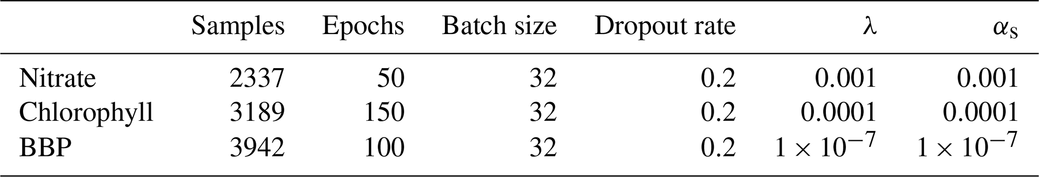
In our experiments, we applied a dropout rate of 0.2, which was consistent across all trained models. This means that, during training, each neuron in the NN has a 20 % chance of being randomly excluded from the computation. Dropout regularization is a technique used to prevent overfitting by encouraging each neuron to encode information independently, thereby inhibiting co-dependencies among neurons.

Table 3 also reports the multiplicative factors that determine the relative contributions of different elements that compose the loss function defined in Sect. 3.3. The values of these hyperparameters vary depending on the variable being inferred, as these variables have different orders of magnitude and result in RMSE values that vary in magnitude as well. It is crucial to accurately balance the regularization term, governed by λ, and the smoothness term, governed by α_s, to prevent them from dominating the loss function's RMSE component. The optimal values reported in Table 3 guarantee a good and smooth prediction of the vertical profile.

The last implementation detail to be addressed concerns the creation of vectors used to feed the PPCon architecture. As previously discussed, vectorial inputs of different natures are fed into the CNN component of PPCon: firstly, the outputs of an MLP architecture; secondly, vectors representing input variables (temperature, salinity, and oxygen) at different depths. To ensure that all input vectors have the same length, we adopted the following strategy: (i) the output and input variables are interpolated on a regular grid of size 200, and (ii) the outputs of MLPs have the same length and discretization of the input variable vectors. For nitrate, we considered a depth range of 0 to 1000 m with an interpolation interval of 5 m, whereas, for chlorophyll and BBP, we considered a depth range of 0 to 200 m with an interpolation interval of 1 m. Then, we set the output layer dimension of the MLP to 200 to ensure that all input vectors have the same length. As a result, the final dimension of the input tensor is 7 (the number of inputs) × 200 (the length of the input vector) × the number of dimensions in the training set.

4.3 A posterior validation analysis of PPCon

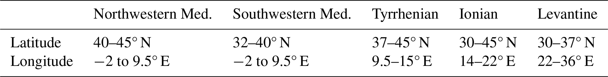
To validate the PPCon architecture, we conducted a thorough analysis of its performance in different geographic areas (NWM, TYR, SWM, ION, and LEV in Fig. 1) and across the four seasons: winter (JFM), spring (AMJ), summer (JAS), and fall (OND). The specific geographical limits related to different areas are also reported in Table 4. While the PPCon model is trained on the entire dataset, this subdivision is only used to analyze the performance retrospectively to check whether the non-uniform geographical and spatial distribution of the profiles and the natural variability in the profiles (e.g., depth and slope of the nitracline or depth and intensity of the DCM) have an influence. In particular, the RMSE is calculated for the reconstructed profiles in each area and season to verify the presence of any bias in the accuracy of PPCon in capturing the spatial and temporal variability in the Mediterranean Sea.

Table 4 Geographical limits of the five areas in which the Mediterranean is divided for the posterior analysis.

5 Results

This section presents the results of the PPCon model in predicting nitrate, chlorophyll, and bbp700 profiles. The effectiveness of the model is evaluated by presenting both quantitative skill metrics (i.e., RMSE) and visual representations of the predicted profiles based on the test set.

Table 5 WMO, date, and geolocation of the float profiles reported in Figs. 1–3.

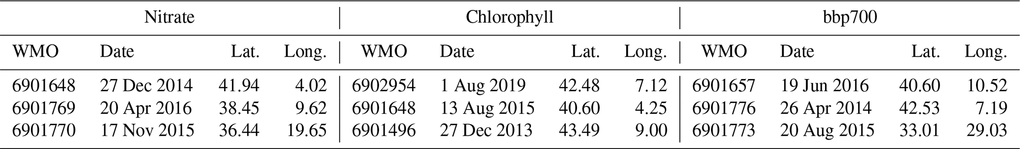
Table 6 RMSE calculated between the float measurements and the reconstructed values obtained from the PPCon architecture. This metric is evaluated individually for the train and test sets. The RMSE is computed for different seasons of the year (described in Sect. 2).

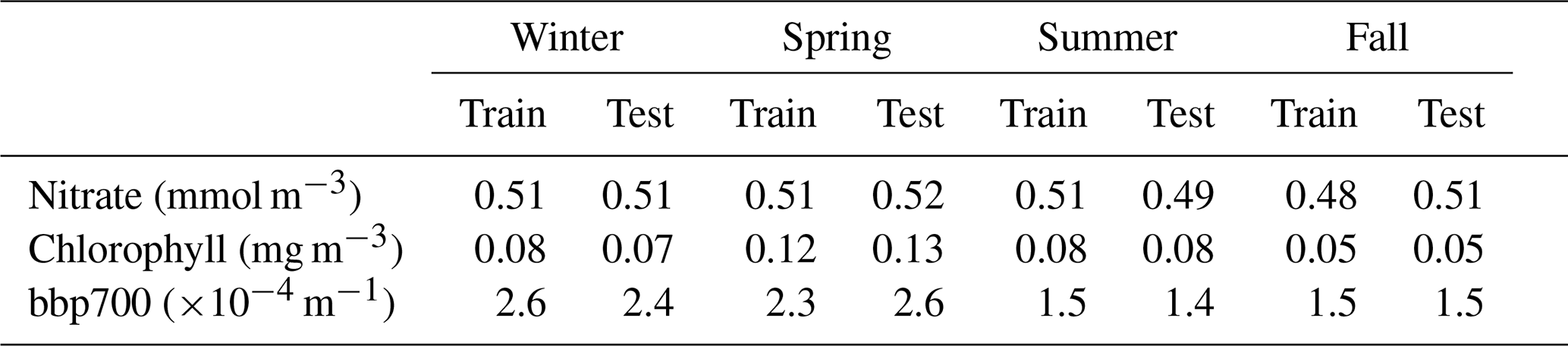
Table 7 RMSE calculated between the float measurements and the reconstructed values obtained from the PPCon architecture. This metric is evaluated individually for the train and test sets. The RMSE is computed for different geographic areas (described in Sect. 2).

Specifically, we assess the PPCon performance over different seasonal variations (Table 6) and different geographic areas (Table 7). The absence of overfitting is supported by reporting the RMSE for both the training and test sets, which exhibit non-dissimilar values.

In terms of performances across different geographic areas (Table 7), it can be seen that the lowest RMSE values for chlorophyll and bbp700 are in the eastern sub-basins, while for nitrate the lowest and highest values are in the two eastern sub-basins. Notably, the prediction accuracy for nitrate is significantly higher in the ION, SWM, and TYR, with RMSE values below 0.5 mmol m⁻³. Considering the temporal evolution of RMSE values (Table 6), the highest values of chlorophyll and bbp700 are in spring and winter, which appears reasonable given the higher variability in the vertical pattern during these seasons (Cossarini et al., 2019; Teruzzi et al., 2021). Errors for nitrate are fairly homogeneous among the seasons, with the highest values during the vertical-mixing season (i.e., winter) and the lowest values during the stratification seasons (i.e., spring and summer). As for chlorophyll, the western basin of the Mediterranean shows higher RMSE values. This can be attributed to the naturally elevated chlorophyll levels observed in that specific area, which consequently lead to higher RMSE values.

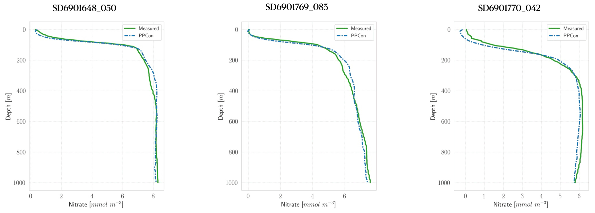
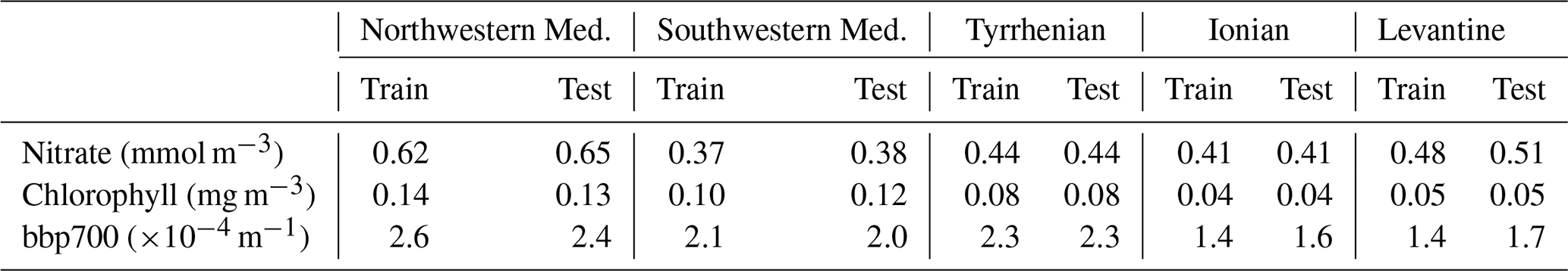
Figure 3 Profiles of nitrate for some selected floats (WMO numbers and cycles in the title). Profile dates and geolocations are reported in Table 5. Comparison between measured profile (green lines) and PPCon reconstruction (dashed blue lines). Profiles are from the subset used for the test.

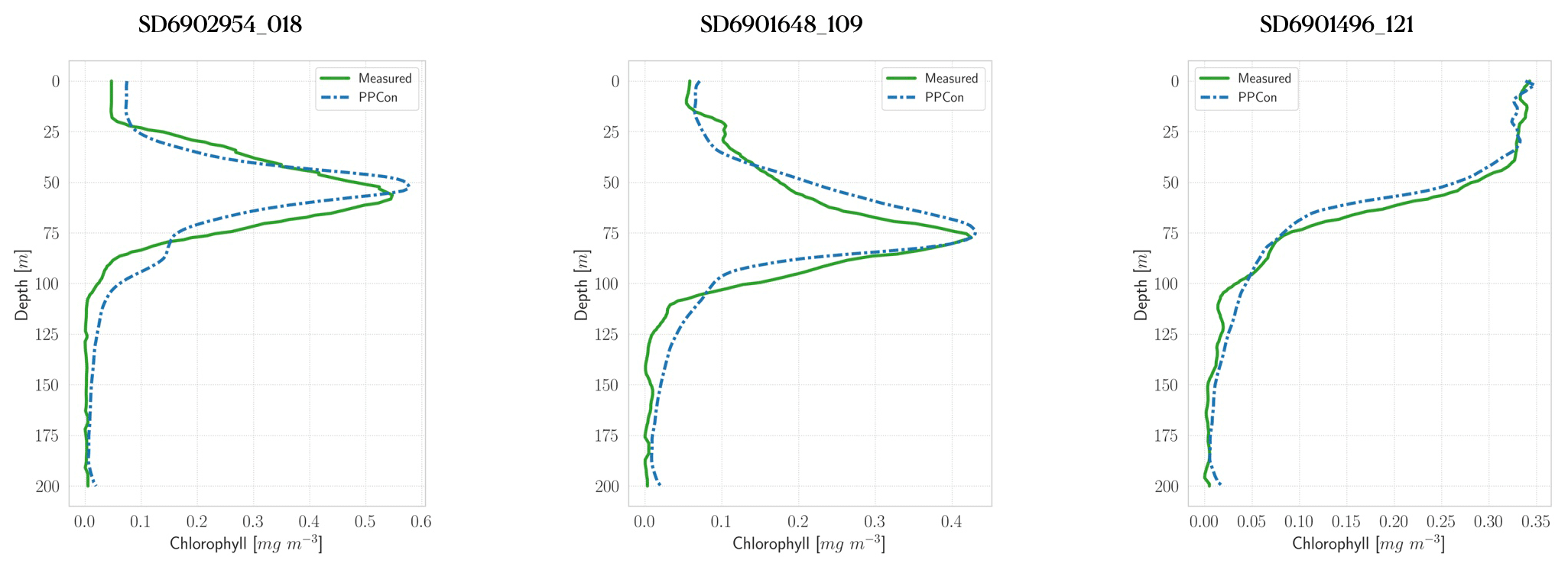
Figure 4 Profiles of chlorophyll for some selected floats (WMO numbers and cycles in the title). Profile dates and geolocations are reported in Table 5. Comparison between measured profile (green lines) and PPCon reconstruction (dashed blue lines). Profiles are from the subset used for the test.

Figure 5 Profiles of bbp700 for some selected floats (WMO numbers and cycles in the title). Profile dates and geolocations are reported in Table 5. Comparison between measured profile (green lines) and PPCon reconstruction (dashed blue lines). Profiles are from the subset used for the test.

For each variable investigated, we present three instances of vertical profile reconstruction using the PPCon architecture compared to the profile measured by the float instrument, whose corresponding identification number is indicated above each profile. To ensure geographic and seasonal diversity, we selected profiles representing different regions, including at least one from the western Mediterranean and one from the eastern Mediterranean. Figures 3–5 display examples of reconstructed nitrate, chlorophyll, and bbp700 profiles, respectively. For the nitrate variable, the reconstruction performed by the MLP model (Pietropolli et al., 2023a; Fourrier et al., 2020) is also reported in Appendix B. The information related to these profiles, such as the date and geolocation of sampling, are reported in Table 5.

The obtained results confirm the quality of the profiles generated by the PPCon architecture, which appears to better reconstruct the shape and smoothness of the profiles than the previous MLP architecture. Indeed, PPCon can capture different profile shapes associated with different geographic and seasonal conditions, as demonstrated by the predicted nitrate and chlorophyll profiles. The visual inspection of all test profiles (not shown) revealed that higher quality in the prediction is achieved for the nitrate variable, followed by chlorophyll, and lastly by bbp700. This outcome is expected, as the nitrate variable exhibits lower variability in the values and profile shapes than chlorophyll and bbp700. For a more detailed analysis of the behavior of the PPCon architecture quality of the predicted profiles, Appendix A reports a comparison between the mean of PPCon-predicted profiles and the mean of profiles measured by the float instruments (in the test set), providing a more specific insight on the PPCon performances in different geographic areas and seasons.

To understand the impact of the training set numerosity and of the variability in profiles on the quality of the PPCon predictions, we investigated the relation between these quantities and the PPCon error. Specifically, Fig. 6 illustrates the RMSE values computed for the reconstructed profiles subdivided into five geographic areas and four seasons. RMSE values, which are indicated by the size of the symbols, are plotted against the variability in the training set (quantified by the standard deviation on the x axis) and the size of the training set (on the y axis). This figure also offers valuable insights into the geographical and seasonal distribution of the training dataset dimension.

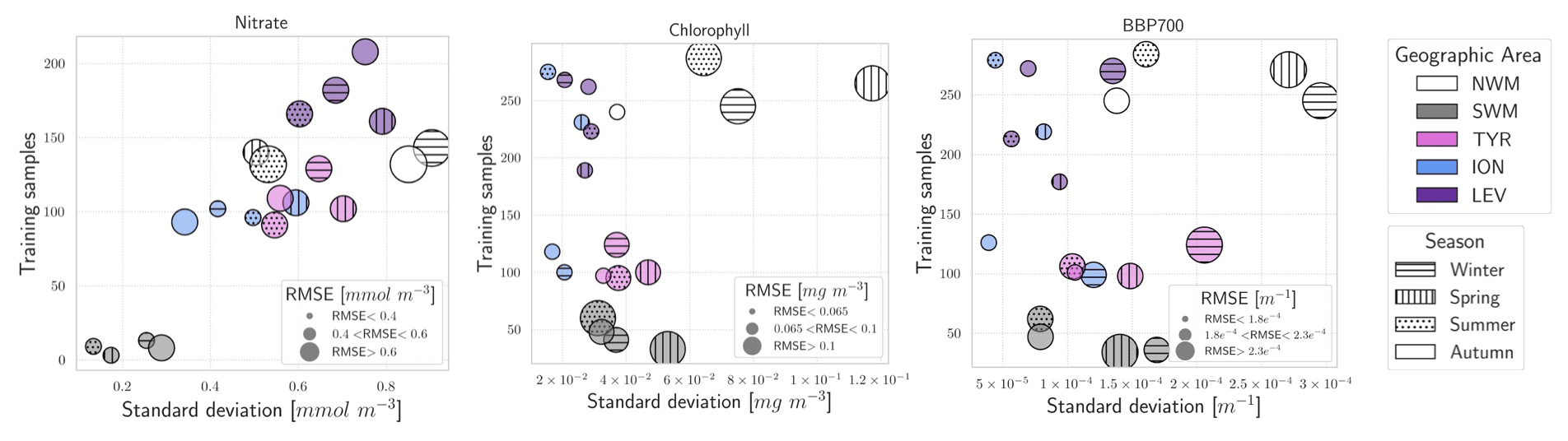
Figure 6 Plot of the RMSE distribution with respect to the data variability (on the x axis) and the training dataset size (on the y axis). Different sub-areas are represented by different symbol colors, and different seasons are represented by different symbol fill patterns. RMSE values are categorized by the size of the symbols, and bigger symbols correspond to bigger RMSE values.

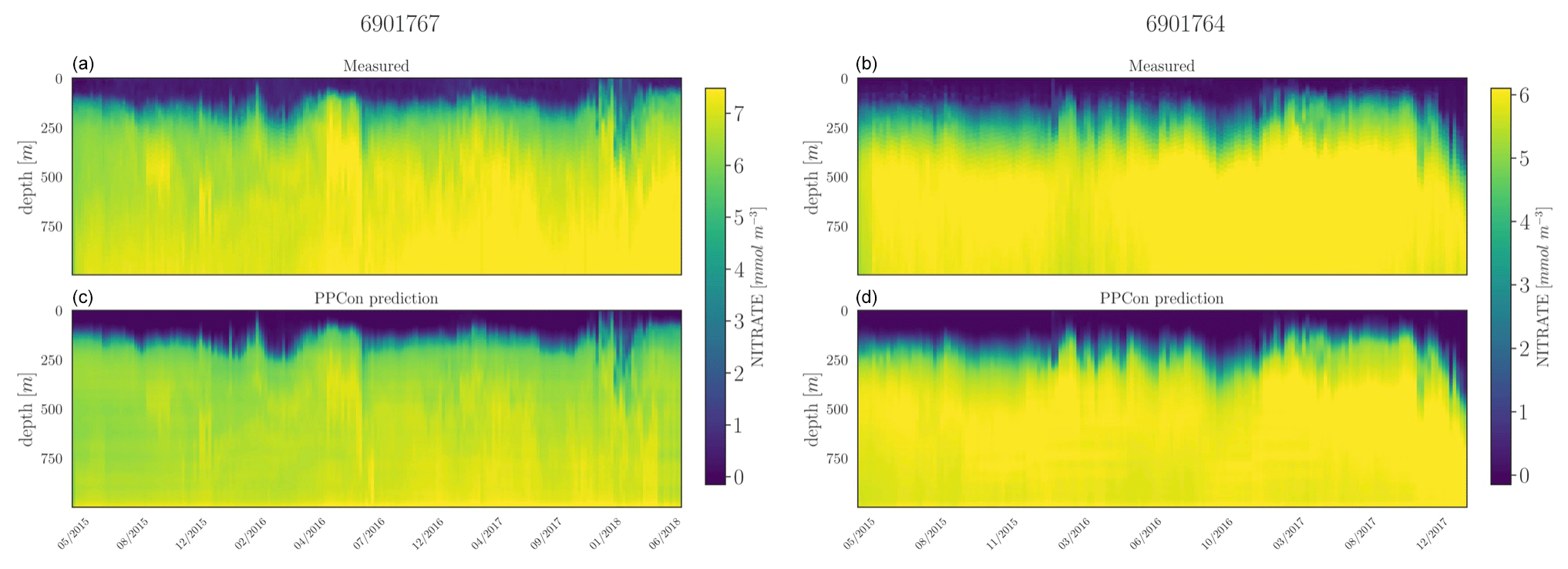
Figure 7 Hovmöller diagrams for the nitrate of two selected floats (WMO name in the title) belonging to the external validation set. BGC-Argo measurements (a, b) and PPCon prediction (c, d) are compared. WMO 6901767 sampled the 39–41° N and 10–11° E area during 2015–2018, whereas WMO 691764 sampled the 31–34° N and 26–40° E area during 2015–2017.

Table 8 RMSE calculated between the float measurements and the reconstructed values obtained from the PPCon architecture over the external validation dataset.

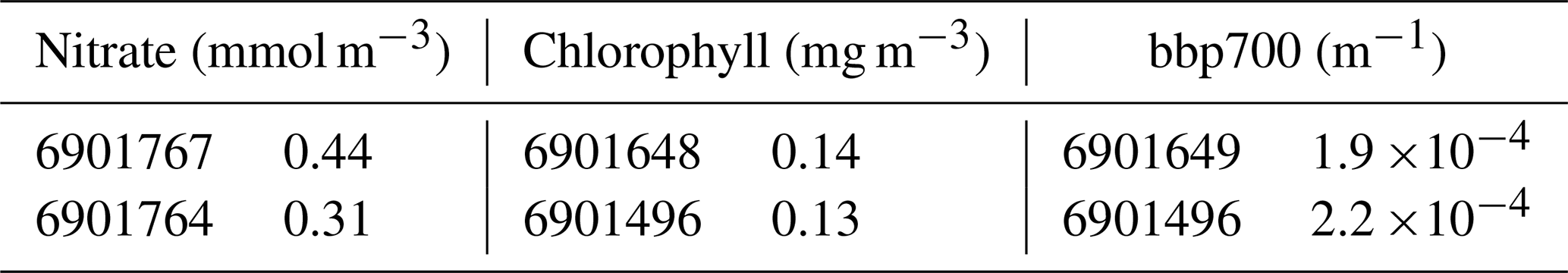
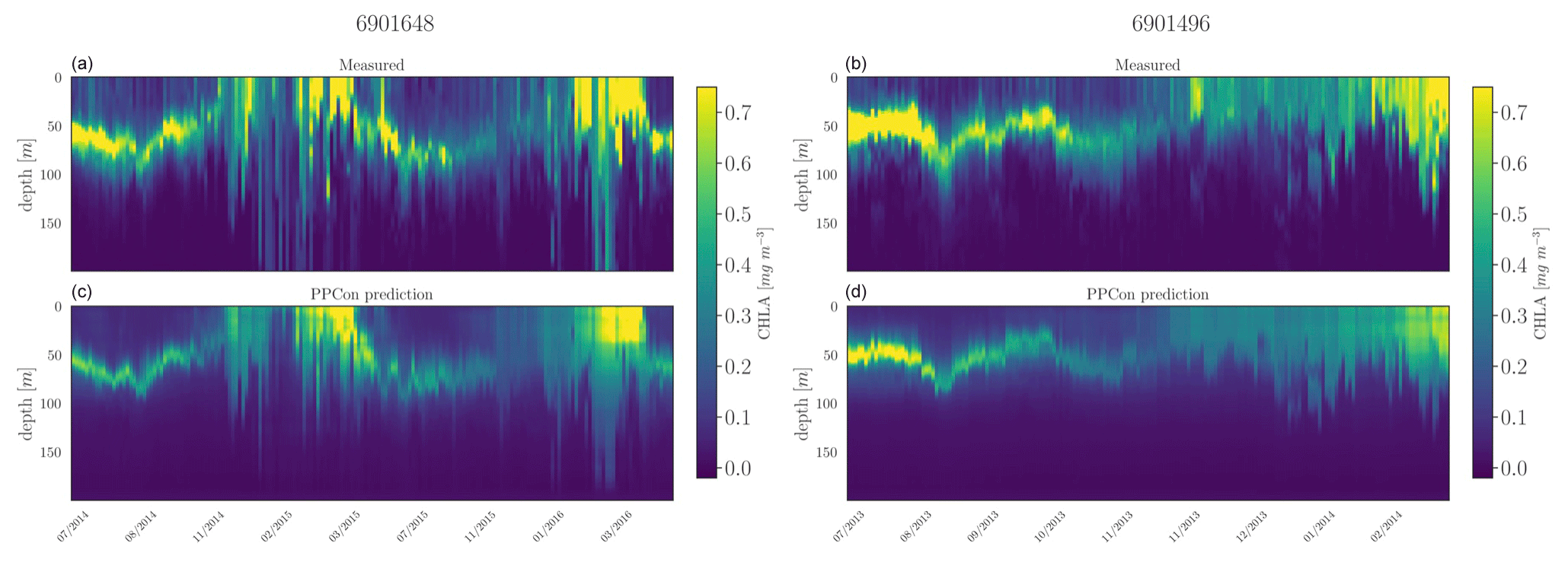
Figure 8 Hovmöller diagrams for the chlorophyll of two selected floats (WMO name in the title) belonging to the external validation set. BGC-Argo measurements (a, b) and PPCon prediction (c, d) are compared. WMO 6901648 sampled the 40–42° N and 2–6° E area during 2014–2016, whereas WMO 6901496 sampled the 42–43° N and 7–12° E area during 2013–2014.

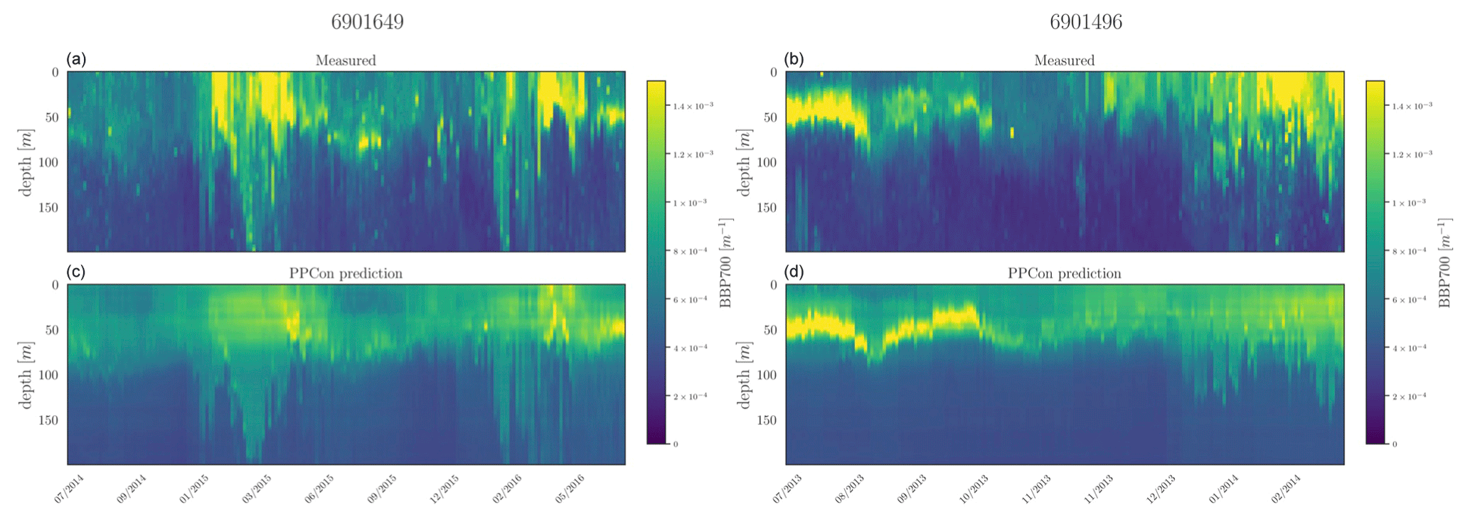
Figure 9 Hovmöller diagrams for the bbp700 of two selected floats (WMO name in the title) belonging to the external validation set. BGC-Argo measurements (a, b) and PPCon prediction (c, d) are compared. WMO 6901649 sampled the 39–41° N and 3–7° E area during 2014–2016, whereas WMO 6901496 sampled the 42–43° N and 7–12° E area during 2013–2014.

In terms of training size, the plots of the three variables show that the SWM exhibits the smallest number of training profiles, while the largest numbers are in the NWM and LEV areas. Natural variability changes across sub-basins with higher values of standard deviations in the western sub-basins (i.e., SWM, NWM, and TYR). Variability and sample size show a roughly homogeneous distribution among seasons.

The analysis of the nitrate plot reveals fairly homogeneous errors across natural variability and training sample size, excluding the SWM profiles. The NWM is the basin predicted with the lowest accuracy, while the SWM and ION generally have the lowest errors. In terms of seasonal variation, the RMSE values appear slightly lower during summer compared to winter and spring.

Chlorophyll and bbp700 exhibit similar behavior (central and right plots in Fig. 6). In particular, data availability appears to have no significant impact on the error, whereas RMSE tends to increase proportionally with the variability.

Regarding the chlorophyll, the performances of the western sub-basins (i.e., NWM, SWM, and TYR) are lower than the eastern sub-basins (LEV and ION), likely due to higher profile variability. Winter and fall are the seasons with lower RMSE, while the highest error is predicted in spring.

Similarly, better performances for bbp700 are observed in LEV and ION compared to in the western sub-basin.

Interestingly, summer and fall performances are almost 50 % better than winter and spring ones, despite the fact that the natural variability and sample size do not show appreciable differences among the seasons.

5.1 PPCon performance over an external validation dataset

For each inferred variable, Figs. 7–9 display Hovmöller diagrams of measured and reconstructed float instruments belonging to the external validation set, and Table 8 reports the corresponding RMSE values. This represents a particularly stringent validation test, since none of the profiles measured by these floats were encountered by the PPCon model during the training or validation phases. The figures compare the in situ float measurements (upper diagram) and the predictions generated by the PPCon architecture (lower diagram) for floats that were specifically selected to cover different geographical regions of the Mediterranean Sea (e.g., one in the eastern and one in the western Mediterranean Sea). White lines in the diagrams indicate float measurements that cannot be compared due to various reasons, such as the sensor's temporary inability to measure the specific variable inferred or the absence of one of the inputs necessary for the PPCon architecture (e.g., at least one between temperature, salinity, and oxygen). This could be attributed to limitations in the sensor or unacceptable quality flags associated with the collected data. Nevertheless, the number of profiles that cannot be calculated by PPCon is rather low and does not degrade the very good capacity of the reconstructed profiles to reproduce the temporal evolution of the vertical dynamics shown by the measured floats.

These plots also confirm the PPCon capability of performing accurate predictions regarding float devices which are totally unseen by the model. The nitrate (Fig. 7) reconstructions exhibit a very good performance of PPCon in predicting the vertical dynamics associated with the temporal evolution of the nutricline depth (i.e., the depth at which the sharp increase in the nitrate values is observed), the values in the deep layers (which are different in the sub-areas sampled by the two floats), and the occurrence of deep vertical mixing when surface concentration increases to values higher than 3 mmol m⁻³. Particularly impressive is the capability of PPCon to reconstruct the temporal dynamics of chlorophyll (Fig. 8). The reconstruction effectively captures the evolution of the chlorophyll surface peaks during winter and the formation of the deep chlorophyll maximum during summer in both floats representing the two areas of the Mediterranean Sea. Among the three variables, bbp700 (Fig. 9) shows the least accurate predictions. However, the model still displays the ability to infer the key characteristics of the variable's temporal behavior. Nonetheless, the generated predictions for bbp700 appear slightly less detailed compared to the original sampling, indicating a partial limitation of the model in capturing small-scale variations.

Quantitatively, the prediction quality of the PPCon architecture (RMSE values in Table 8) is fairly well aligned with the metrics calculated over the test set, as indicated in Table 7. In particular, nitrate errors of the two floats are quite homogeneous and 30 % lower than the RMSE values of the test set. The errors in chlorophyll and bbp700 predictions exhibit greater variability, with values almost double for the floats in the western Mediterranean with respect to the eastern ones. This is, however, in line with results reported in Table 7 and Fig. 6, where higher errors are associated with higher variability.

6 Discussion

To our knowledge, the PPCon architecture is the first attempt to predict vertical BGC-Argo profiles through a convolutional architecture. Its primary objective is the incorporation of typical profile shapes during the training phase, in contrast with previous architectures, which all relied on MLP architectures and point-wise strategy. There are notable distinctions between the two approaches: MLPs were trained on cruise data, which are known to be more precise in collecting data than autonomous sensors such as the BGC-Argo (Johnson et al., 2013; Johnson and Claustre, 2016). However, while MLP architectures have been demonstrated to provide good training and test errors for point-wise input and output (Pietropolli et al., 2023a; Fourrier et al., 2020; Bittig et al., 2018; Sauzède et al., 2017), they can exhibit higher errors when predicting BGC-Argo profiles, as demonstrated in Pietropolli et al. (2023a) and Appendix B. In contrast, the PPCon architecture, which relies directly on BGC-Argo float measurements for the training, showed very good test and external validation performances.

However, it should be noted that an intrinsic measurement error is introduced by the higher uncertainty in the variables measured throughout the autonomous sensors. We alleviated this limitation by using only DT and high-quality Argo and BGC-Argo float data that had been checked; however, the use of the present PPCon in operational oceanography (Le Traon et al., 2021; Cossarini et al., 2019) should be considered cautiously given the lower reliability of adjusted or near-real-time (NRT) Argo data. According to the analysis conducted by Mignot et al. (2019), the BGC-Argo float data for nitrate and chlorophyll exhibit RMSE values evaluated at 0.25 mmol m⁻³ and 0.03 mg m⁻³, respectively. On the other hand, PPCon architecture produced BGC-Argo profile reconstruction with RMSE values of 0.52 mmol m⁻³ and 0.08 mg m⁻³ for nitrate and chlorophyll, respectively. Therefore, a research question remains as to how the measurement error of the float instrument impacts the performance of the PPCon architecture and how to estimate an overall error that combines the contribution of the instrument error and the error associated with the PPCon.

Although both MLPs and PPCon employ similar input information (date, geolocation, temperature, oxygen, and salinity), their treatment of these data differs significantly. While the current MLP applications process the input and output as point-wise data, PPCon utilizes vector representations of the vertical profiles. This approach effectively exploits the potential of a 1D CNN, which intrinsically preserves the characteristic profile shape of the input and output variables (Kiranyaz et al., 2021). When comparing the predictive performance of these techniques in generating vertical profiles from float data, distinct differences emerge. MLPs can produce profiles affected by artificial discontinuity, while the profiles generated by PPCon exhibit a smoother and more realistic appearance (Appendix B). Additionally, the RMSE values computed on the reconstructed nitrate profiles of the test subset confirm the better performance of the 1D CNN approach with respect to an MLP approach trained on point-wise data (Appendix B).

Moreover, the posterior study that we conducted shows that there is no significant variation in the error across different geographic areas and seasons of the year (Tables 6–7), confirming that PPCon can successfully be applied to all of the float profiles collected in the Mediterranean Basin.

Specifically, the PPCon architecture serves as a valuable tool for significantly enriching the BGC-Argo dataset. This becomes useful, as ocean-observing systems, while essential for monitoring the health of the marine ecosystem (Euzen et al., 2017), have considerable limitations given their sparse and scarce spatiotemporal coverage. Surface satellite observations are limited by cloud coverage and incomplete swaths of satellite sensors (Donlon et al., 2012), while profiling the ocean interior is limited by the capacity of deploying and retrieving sensors and measurements with sufficient coverage. Gap-filling and interpolation of satellite observations (Volpe et al., 2018; Sammartino et al., 2020; Alvera-Azcárate et al., 2005) are nowadays consolidated practices to provide gap-free and high-level products (Barth et al., 2020; Sauzède et al., 2016). Our PPCon architecture presents a valuable approach to harness the potential of the Argo and BGC-Argo network by enabling the synthetic generation of essential variables (chlorophyll, nitrate, and bbp700), even when these costly sensors are not present in the deployed floats. For instance, the application of PPCon on Argo and oxygen profiles in the Mediterranean Sea for the period from 2013 to 2020 enabled the generation of 5234 (nitrate), 3879 (chlorophyll), and 3307 (bbp700) synthetic profiles, which means doubling the chlorophyll and bbp700 BGC-Argo profiles and more than tripling those of nitrate. Enhancing the float dataset through the inclusion of reconstructed nutrient profiles (and possibly other biogeochemical variables) has been proven successful in observing system simulation experiments (Ford, 2021; Yu et al., 2018) and in real numerical assimilation experiments (Amadio et al., 2024). In particular, the assimilation of reconstructed profiles effectively corrects a widespread positive bias observed in the operational system for short-term forecasting of the biogeochemistry of the Mediterranean (MedBFM), along with the addition of the reconstructed profiles increasing the spatial impact of the BGC-Argo network from 20 % to 45 % (Amadio et al., 2024).

7 Conclusions

This paper presents a novel approach for reconstructing low-sampled variables, namely nitrate, chlorophyll, and bbp700, using high-sampled variables such as date, geolocation, temperature, salinity, and oxygen. The introduced model, named PPCon, utilizes a spatially aware 1D CNN architecture that effectively learns the characteristic shape of the vertical profile, enabling precise and smooth reconstructions. PPCon represents a potential advancement in predicting BGC-Argo profiles over previous MLP applications, which operate on point-wise input and output.

The training dataset consists of a collection of BGC-Argo float measurements in the Mediterranean Basin. The proposed architecture has been specifically designed to handle both point-wise and vectorial input, with careful tuning of the architecture and loss function for the task. An extensive hyperparameter-tuning phase has been conducted to ensure the best architecture for each variable.

To evaluate the accuracy of the profiles generated by the PPCon architecture, both quantitative metrics and visual representations of the results have been provided. Additionally, the method has been validated on an external dataset to verify its generability. The results confirm the model's ability to predict high-quality synthetic profiles, with particularly accurate predictions for the nitrate variable, followed by chlorophyll and, lastly, bbp700.

PPCon demonstrates its capacity to capture and learn distinct typical shapes in the profiles, which characterize the inferred variables across different seasons and geographic areas. Detailed error analysis confirms the model's robust performance, accounting for seasonal and regional variations, suggesting that PPCon's ability to learn these differences can make it successful for broader-scale training beyond the Mediterranean Basin. Furthermore, the model exhibits accurate performance on an external validation dataset, confirming its potential for generalization.

Appendix A: Extended results

Figure A1 presents a comparison between the mean values of the PPCon predicted profiles and the mean values of the sampled measurements obtained from the float instruments in the test set. The mean values are computed based on the profiles within a specific geographic area and season. These profiles serve as additional indicators to assess the reliability of predictions within different frameworks, providing valuable insights into the precision of predictions at various depth levels. These results confirm the previous observations discussed in Sect. 5, particularly the finding that the prediction quality is superior for the nitrate, followed by chlorophyll and, lastly, bbp700. Additionally, an interesting characteristic of the PPCon prediction is its higher quality in deep water compared to surface water. This can be attributed to the higher variability in profiles in the surface water, making it more challenging for the neural network to accurately capture the diverse shapes.

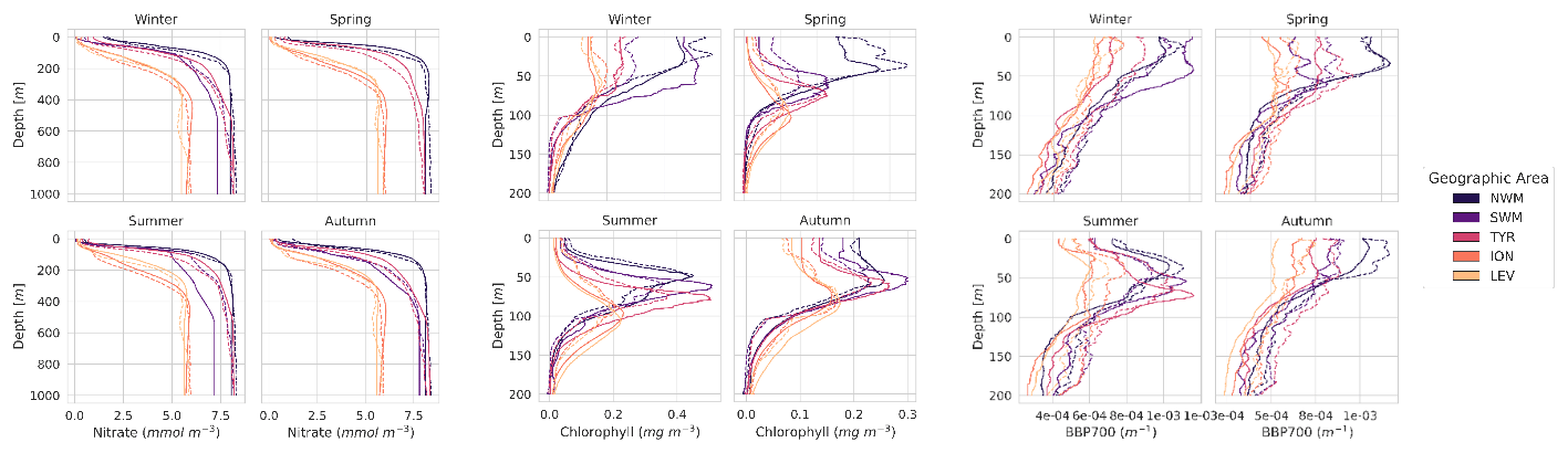
Figure A1 Comparison of the mean of PPCon predicted profiles with the mean of sampled values measured by the float instruments in the test set. Results are divided among different geographic areas: the dashed lines represent sampled values, while continuous lines represent PPCon predictions.

Appendix B: Comparison between reconstructed nitrate profiles by PPCon and MLP architectures

The present appendix aims to show the performance of three different ML architectures to reconstruct nitrate profiles that use Argo profiles of temperature and salinity and BGC-Argo profiles of oxygen. The three ML architectures are the 1D CNN of the present work (PPCon), MLP trained on point-wise data from EMODnet (Pietropolli et al., 2023a), and MLP trained on point-wise data (Fourrier et al., 2020). Input data from Argo and BGC-Argo for all approaches have been interpolated to the regular 5 m discretization, as explained in Sect. 4. The comparison is done on the subset of profiles used in the test phase. Figure B1 shows some measured and reconstructed float profiles. The visual comparison reveals the higher performance of PPCon to match the shape of the measured profiles (e.g., depth and intensity of the nitracline) and to reproduce the nitrate values of the deepest part of the profiles observed in the different Mediterranean sub-regions. The quantitative assessment of the performance of the three ML architectures is shown in Table B1, which reports the RMSE computed over all profiles of the subset used in the test phase. The RMSE of the reconstructed profile by PPCon is more than 30 % lower than that computed on the MLP reconstructions.

(Fourrier et al., 2020)(Pietropolli et al., 2023a)

Table B1 RMSE of the three ML architectures computed over the nitrate profiles of the subset BGC-Argo dataset of the test phase.

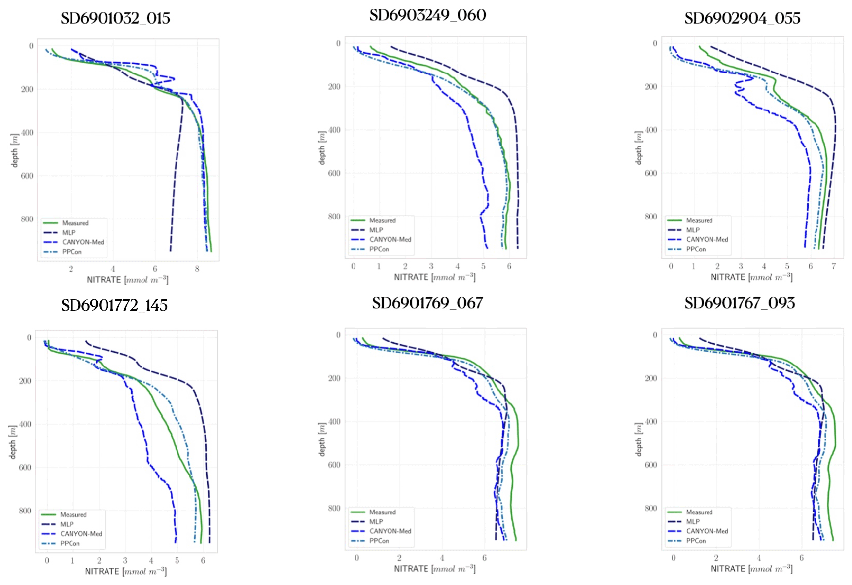
Figure B1 Nitrate profiles from the BGC-Argo dataset (green, measured) and reconstructed by PPCon (dashed cyan line), MLP as in (Pietropolli et al., 2023a) (dashed purple line) and CANYON-MED (dashed dark-blue line). Profiles are selected from the subset used in the test phase of the present work. Float positions are as follows: 6901032 in NWM, 6903249 and 6901772 in ION, 6902904 in LEV, 6901767 in TYR, and 6901769 in SWM.