the Creative Commons Attribution 4.0 License.
the Creative Commons Attribution 4.0 License.
 | 25 Sep 2024
Methane dynamics in the Baltic Sea: investigating concentration, flux, and isotopic composition patterns using the coupled physical–biogeochemical model BALTSEM-CH4 v1.0
Bo G. Gustafsson
Martijn Hermans
Christoph Humborg
Christian Stranne
Methane (CH4) cycling in the Baltic Sea is studied through model simulations that incorporate the stable isotopes of CH4 (12C–CH4 and 13C–CH4) in a physical–biogeochemical model. A major uncertainty is that spatial and temporal variations in the sediment source are not well known. Furthermore, the coarse spatial resolution prevents the model from resolving shallow-water near-shore areas for which measurements indicate occurrences of considerably higher CH4 concentrations and emissions compared with the open Baltic Sea. A preliminary CH4 budget for the central Baltic Sea (the Baltic Proper) identifies benthic release as the dominant CH4 source, which is largely balanced by oxidation in the water column and to a smaller degree by outgassing. The contributions from river loads and lateral exchange with adjacent areas are of marginal importance. Simulated total CH4 emissions from the Baltic Proper correspond to an average ∼1.5 mmol CH4 m−2 yr−1, which can be compared to a fitted sediment source of ∼18 mmol CH4 m−2 yr−1. A large-scale approach is used in this study, but the parameterizations and parameters presented here could also be implemented in models of near-shore areas where CH4 concentrations and fluxes are typically substantially larger and more variable. Currently, it is not known how important local shallow-water CH4 hotspots are compared with the open water outgassing in the Baltic Sea.
- Article
(2182 KB) - Full-text XML
-
Supplement
(2656 KB) - BibTeX
- EndNote


Methane is the second most important greenhouse gas after carbon dioxide (CO2), contributing about 20 % of the total radiative forcing (Etminan et al., 2016). Using top-down approaches (atmospheric observations and inverse modeling), the present-day global CH4 emissions have been estimated to be 576 Tg CH4 yr−1 (range: 550–594), whereas bottom-up approaches (process-based modeling of land surface emissions and data on anthropogenic emissions) yield a total of 737 Tg CH4 yr−1 (range: 594–881; Saunois et al., 2020). The causes of the discrepancy between the two methods are not well known, but the discrepancy is believed to mainly reflect uncertainties in estimates of natural emissions – in particular from wetlands, lakes, and running waters (Saunois et al., 2020). The global mean atmospheric CH4 level has increased by about 1000 ppb over the last 2 centuries (Ferretti et al., 2005). Projections of future development range from a gradual decrease to a massive increase, depending on the development of anthropogenic emissions (Saunois et al., 2020).
The isotopic composition of atmospheric CH4 () varies seasonally and over longer timescales (Ferretti et al., 2005; Lan et al., 2021). Long-term trends of depend on the relative contributions from three main sources: biogenic (−110 ‰ to −50 ‰; e.g., wetlands −60 ‰); fossil (−40 ‰); and pyrogenic/biomass burning (−25 ‰ or −12 ‰; depending on pathways of carbon fixation in plants). Over the 20th century, a long-term increase in from −49 ‰ to −47 ‰ occurred (Ferretti et al., 2005). However, a recent increase in the atmospheric CH4 level has been accompanied by a decrease in , for reasons that are not fully understood (Lan et al., 2021). The observed development can help to constrain different CH4 sources and thus reduce their uncertainties.
It has been estimated that approximately half of the total CH4 emissions come from aquatic ecosystem sources, dominated by inland water ecosystems (Rosentreter et al., 2021). The total oceanic CH4 emissions, including diffusive and bubble-driven ebullitive fluxes, constitute a relatively small fraction amounting to ∼6–12 Tg CH4 yr−1 (Weber et al., 2019). Methane formation in sediments can be substantial, but aerobic and anaerobic oxidation processes can efficiently remove CH4 both in the pore water and water column. For that reason, near-shore areas (0–50 m water depth), shallow enough to allow CH4 to escape to the atmosphere before being oxidized, dominate the oceanic emissions despite representing a comparatively minor area (Weber et al., 2019). In shallow, organic-rich sediments, seafloor ebullition will increase in response to ocean warming due to increased biogenic CH4 production and decreased CH4 solubility (Borges et al., 2016). This notion was qualitatively supported by acoustic observations of outgassing from the sediments during a recent field study, where exceptionally high CH4 emissions were reported from the coastal Baltic Sea at the end of a summer heat wave (∼250 ; Humborg et al., 2019).
The coastal ocean is currently a net CO2 sink, which depending on the method (observations or model calculations) has been estimated to be approximately 0.44–0.72 Pg C yr−1 (Resplandy et al., 2024). Emissions of the powerful greenhouse gases nitrous oxide (N2O) and CH4 can, however, offset the CO2 uptake in the net radiative balance of the coastal ocean: while highly uncertain, preliminary estimates indicate an offset in the range 30 %–60 % (Resplandy et al., 2024). These numbers highlight the crucial importance of more accurate estimates of both N2O and CH4 fluxes from coastal areas when determining the influence of the coastal ocean on climate.
In the Baltic Sea, there are strong gradients in CH4 concentrations both from near-shore areas to open Baltic Sea surface waters (e.g., Gülzow et al., 2013; Humborg et al., 2019) and from surface to deep waters (e.g., Schmale et al., 2010; Jakobs et al., 2013). Substantial parts of Baltic Sea deep waters are stagnant over extended periods in time, which in combination with high loads of organic material cause episodic anoxia (e.g., Carstensen et al., 2014). During stagnant anoxic periods, CH4 accumulates and reaches concentrations ranging from 1000 to 3000 nM (Jakobs et al., 2013, 2014; Ketzer et al., 2024). This CH4 is, however, largely consumed by aerobic oxidation processes (MOX) when mixed into the redoxcline at intermediate depths (Jakobs et al., 2013). Peak oxidation rates have consequently been observed in the redoxcline, where deep water rich in CH4 is mixed with oxic water (Jakobs et al., 2013). Due to the special characteristics of deep-water areas isolated from the atmosphere, and with transitions between oxic and anoxic conditions, the Baltic Sea is a unique and suitable system for studying key processes in CH4 cycling, in particular for investigating different oxidation pathways.
Surface water CH4 concentrations in the open Baltic Sea are typically about 3.5–5 nM – only slightly oversaturated compared with the atmosphere (Gülzow et al., 2013). By contrast, in shallow near-shore areas, observations indicate a very different situation, with CH4 concentrations ranging from 10 to 500 nM (Humborg et al., 2019; Myllykangas et al., 2020; Lundevall-Zara et al., 2021; Roth et al., 2022) and with large temporal and spatial variations on small scales (e.g., Roth et al., 2022). Methane emissions to the atmosphere depend on the degree of oversaturation in the surface water but also on wind speed and temperature (e.g., Wanninkhof, 2014). Estimated CH4 emissions from different near-shore sites in the Baltic Sea display a large range due to substantial variations in the parameters that control gas transfer across the air–sea interface (Humborg et al., 2019; Lundevall-Zara et al., 2021; Asplund et al., 2022; Roth et al., 2022, 2023). Short-term and small-scale variations cause considerable challenges for empirical estimates of fluxes over larger scales and longer periods in time.
Different processes in CH4 cycling do, however, produce certain “fingerprints” on the isotopic composition, similar to how the relative contributions of different atmospheric CH4 sources determine long-term trends of (Lan et al., 2021). This can be helpful when assessing process rates. Observations in the Baltic Sea show a pronounced 13C–CH4 enrichment in the redoxcline (Schmale et al., 2012, 2016; Jakobs et al., 2013, 2014; Gülzow et al., 2014), which is the result of a preferential oxidation of the lighter isotope. Similarly, CH4 emissions to the atmosphere can produce a 13C–CH4 enrichment in the surface water because of a preferential outgassing of the lighter isotope (Knox et al., 1992). The isotopic composition of CH4 produced in sediments depends on the processes involved, i.e., CO2 reduction or acetate fermentation (Reeburgh, 2007; see also Sect. 2.3.5), but it can then be modified by oxidation processes in the pore water (Chuang et al., 2019).
Models can be useful for identifying limiting processes and constraining budgets – even though not all rates are well known – through sensitivity experiments on process rates and parameterizations as well as on the influence of changes in forcing of the system. Methane cycling has previously been investigated in both lake (e.g., Lopes et al., 2011; Greene et al., 2014; Tan et al., 2015; Stepanenko et al., 2016; Bayer et al., 2019) and ocean (e.g., Nihous and Masutani, 2006; Wåhlström and Meier, 2014; Malakhova and Golubeva, 2022) modeling studies. In the present study, CH4 cycling and dynamics in the Baltic Sea are introduced into the coupled physical–biogeochemical Baltic Sea long-term and large-scale eutrophication model (BALTSEM), by expanding with state variables for both 12C–CH4 and 13C–CH4 concentrations (see Sect. 2.2). BALTSEM has previously been used in a similar approach, where stable isotopes of dissolved inorganic carbon as well as dissolved and particulate organic carbon were included in the model in order to investigate constraints on process rates (Gustafsson et al., 2015).
Benthic CH4 release and the isotopic composition of CH4 produced in the sediments are not well known, except for a few specific sites where in situ measurements have been acquired. This means that the model is, at this point, somewhat poorly constrained. The main objective of this study is to use the model in concert with observed water column CH4 concentrations and isotopic compositions to (1) identify and roughly quantify key CH4 fluxes, (2) set up a preliminary CH4 budget for the Baltic Proper (where measured profiles of CH4 concentration and isotopic composition are available), and (3) perform sensitivity experiments on CH4 concentration and isotopic composition depending on transport and transformation processes.
The motivation for implementing CH4 modeling on a large scale – with considerable spatial differences in terms of, e.g., water and sediment properties as well as production, respiration, and sedimentation patterns – was utilizing the application of an already well-established model. BALTSEM has been described and validated in many publications, and it has been demonstrated that both physical (e.g., salinity, temperature, vertical mixing, lateral exchange, air–sea exchange) and biogeochemical (e.g., carbon and nutrient cycling and oxygen production/consumption) processes are largely satisfactory (Gustafsson et al., 2012, 2017; Savchuk et al., 2012).
2.1 Area description
The Baltic Sea is a semi-enclosed brackish sea, connected to the North Sea via the shallow and narrow Danish straits. The system is characterized by a pronounced horizontal salinity gradient – going from the almost oceanic entrance area to the low-saline northernmost sub-basin – as well as by permanent salt-dominated stratification, restricted water exchange with the North Sea, and long residence times (e.g., Stigebrandt and Gustafsson, 2003). As a result of strong stratification and long residence times, the central Baltic Sea is naturally susceptible to deep-water de-oxygenation. Massively increased nitrogen (N) and phosphorus (P) loads from the early 1950s to the mid-1980s caused a large expansion of de-oxygenated deep-water areas (e.g., Gustafsson et al., 2012). The loads have declined substantially from the peak values in the 1980s (e.g., Kuliński et al., 2022), although oxygen conditions have not yet improved in the central Baltic Sea (Hansson and Viktorsson, 2023).
2.2 The model
BALTSEM is a horizontally averaged but vertically resolved process-oriented model that couples hydrodynamic and biogeochemical modules in time-dependent, numerical simulations. In the model, the Baltic Sea is divided into 13 coupled sub-basins (Fig. S1 in the Supplement), with geometric characteristics as summarized in Table S1 in the Supplement. The hydrodynamic module has been described in detail by Gustafsson (2000, 2003), while the biogeochemical module has been described in detail by Savchuk (2002). The two modules are qualitatively recapped in Sects. 2.2.1 and 2.2.2.
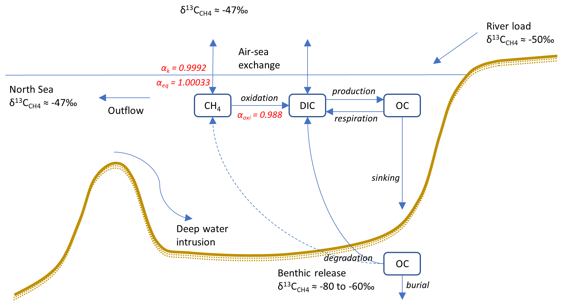
Figure 1Conceptual sketch illustrating the processes involved in CH4 cycling, including values of end-members as well as α values of transformation processes (see Sect. 2.3). The benthic release (dashed arrow) is not explicitly modeled, but instead a preset fitted value is used (see Sect. 2.3.5).
In this study, a new expanded version of the model, BALTSEM-CH4 v1.0, with state variables representing both 12C–CH4 and 13C–CH4 (Gustafsson and Gustafsson, 2023) is presented for the first time. Figure 1 illustrates the processes involved in CH4 cycling that are included in the model. This study focuses on the modeling of stable CH4 isotopes: the CH4 sources (i.e., river load and sediment release); boundary conditions (i.e., atmospheric CH4 and CH4 at the open-ocean boundary); transport and transformation processes (i.e., CH4 oxidation and air–sea exchange); and the isotopic fingerprints associated with these processes are described in Sect. 2.3. The model parameterizations for both hydrodynamic and biogeochemical processes (prior to the inclusion of CH4) have been described in detail in earlier publications (e.g., Gustafsson 2000, 2003; Gustafsson et al., 2012; 2014, 2017; Savchuk, 2002; Savchuk et al., 2012); this will not be repeated here. A list of all state variables in the model is included in Appendix A (Table A1).
2.2.1 Hydrodynamic module
The vertical stratification in each sub-basin is resolved by a variable number of horizontally homogeneous layers. The numbers of layers in the respective sub-basins increase over time because of both inflows from adjacent basins and instances of pycnocline retreat, as described below, but they are kept below maximum values by mixing of the two layers that require the least amount of energy to be merged (Gustafsson, 2000).
Flow dynamics through the straits that connect different sub-basins depends on the width of the strait compared to the internal Rossby radius, determining whether or not earth rotation influences the water exchange. In general, lateral exchange between sub-basins is forced by barotropic pressure gradients across the straits that depend on the sea level difference and wind set-up as well as by baroclinic pressure gradients caused by differences in stratification. In narrow straits, the water flow is influenced by frictional resistance and dynamical contraction due to the Bernoulli effect, while the transport through wider straits is further controlled by earth rotation effects (Gustafsson, 2000, 2003).
The dynamics of the mixed surface layer in each sub-basin is forced by wind stress and buoyancy fluxes but also depends on earth rotation, following Stigebrandt (1985). The pycnocline is eroded whenever the buoyancy flux is negative (e.g., if surface water density increases because of net evaporation, or by cooling when the water temperature is above the temperature for maximum density) or when the buoyancy flux is positive but the power generated by wind stress is sufficient to do work against the buoyancy forces. Pycnocline erosion means that the mixed surface layer becomes thicker and denser as a result of deep-water entrainment into the surface layer. If the power is not sufficient, the turbulent mixing becomes limited either by earth rotation or by buoyancy fluxes, leading to a pycnocline retreat and the formation of a new and shallower mixed surface layer. The thickness of the new surface layer will be determined either by the Ekman or Monin–Obukhov length scale – whichever is shorter (Stigebrandt, 1985).
Entrainment flows are further modified by the presence of sea ice (Gustafsson, 2003). Ice dynamics is based on a sea-ice model by Björk (1997) but adapted to the Baltic Sea following Nohr et al. (2009). Calculations for heating/cooling and evaporation at the sea, ice, or snow surface follow Björk (1997). About half of the incoming shortwave radiation is absorbed at the surface, while the remaining fraction attenuates exponentially using constant attenuation factors for water, ice, and snow.
Turbulent vertical diffusion in deeper layers below the mixed surface layer is parameterized as a function of stratification and mixing wind (Stigebrandt, 1987; Axell, 1998), representing the energy inputs from inertial currents and breaking internal waves. The model further includes dense gravity currents (i.e., deep-water inflows along the seafloor), where entrainment of surrounding deep water into the gravity currents depends on the bottom slope and friction as well as on the density difference between the gravity current and the surrounding water (Stigebrandt, 1987). Entrainment of surrounding water into gravity currents has the effect that the volume flow increases while at the same time density decreases, influencing at what depth the gravity current will be interleaved, i.e., the depth of neutral buoyancy. Deep-water inflows cause an uplift of the entire water column above the intrusion depth.
2.2.2 Biogeochemical module
Biogeochemical processes are calculated using a nutrient–phytoplankton–zooplankton–detritus model set-up that closely follows Savchuk (2002) but that has been expanded with state variables representing, e.g., dissolved organic compounds and the inorganic carbon system (Gustafsson et al., 2014).
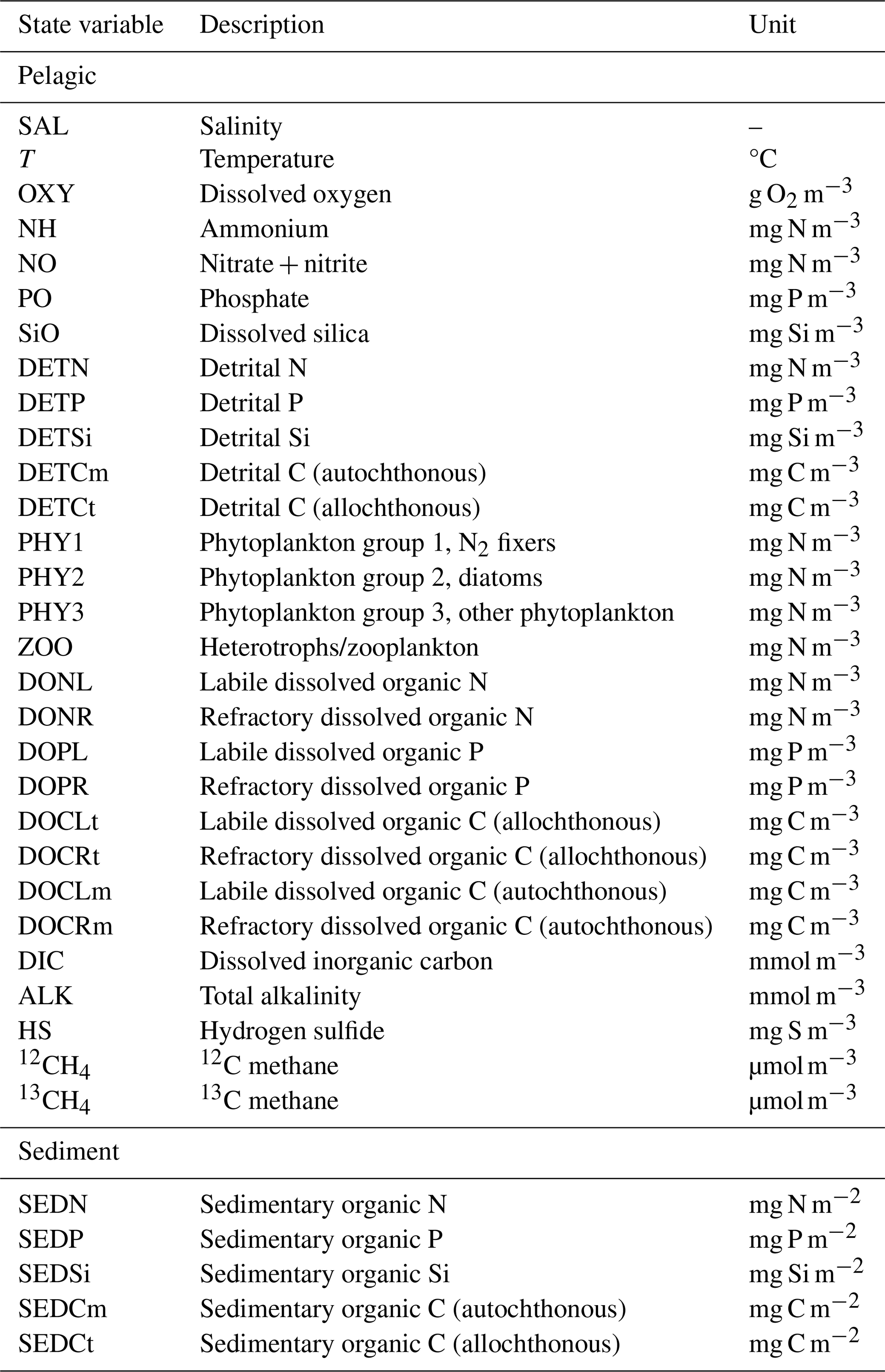
The biogeochemical module includes pelagic state variables for oxygen (O2); hydrogen sulfide (H2S); total alkalinity; dissolved inorganic carbon; nitrate + nitrite; ammonium; phosphate; dissolved silica; labile and refractory fractions of dissolved organic carbon (C), nitrogen (N), and phosphorus (P); particulate organic C, N, P, and silicon (Si); three functional groups of phytoplankton (representing diatoms, “summer species”, and diazotrophic cyanobacteria); and one bulk state variable for heterotrophs that represents zooplankton and other organisms that consume and mineralize phytoplankton and detrital matter. All pelagic state variables are subject to transport processes (vertical mixing and horizontal advection) as well as various biological and chemical transformation processes; source and sink terms for each state variable are computed in all water layers in each sub-basin. BALTSEM further includes sediment pools of C, N, P, and Si that are subject to mineralization and burial. The pelagic and benthic realms are coupled by sedimentation of organic matter and sediment–water exchange of dissolved inorganic compounds. Oxygen, CO2, and CH4 are exchanged at the air–sea boundary depending on solubilities, wind speed, and gradients between the sea surface and air of the respective gases.
Phytoplankton growth depends on water temperature and is further limited by light and nutrient availability (Savchuk, 2002). Light penetration in water in the biogeochemical module is calculated as a function of the biogeochemical state. The phytoplankton groups assimilate dissolved inorganic C, N, and P according to fixed Redfield ratios while at the same time producing oxygen, but they also take up an excess of dissolved inorganic carbon, which is transformed into dissolved organic carbon, representing extracellular production (Gustafsson et al., 2014). The cyanobacteria group is able to fix atmospheric N when ammonium and nitrate become limiting. The diatom group is the only phytoplankton group that requires dissolved silica. Loss terms for phytoplankton include natural mortality, grazing by zooplankton, and sinking. Dead phytoplankton are converted into detrital C, N, P, and Si according to their elemental stoichiometry.
Heterotroph/zooplankton growth depends on the grazing rate, which is regulated by water temperature and food concentration (phytoplankton and detritus), as well as the respective availability of different food sources (Savchuk, 2002). Grazing is in addition strongly inhibited at low oxygen concentrations. Fractions of each food source that are not digested are instead assigned to detritus pools in accordance with the stoichiometry of the food sources. Zooplankton have elemental stoichiometry that differs from their food sources; growth thus becomes limited by the element in relative shortage, while carbon and nutrients in excess of zooplankton stoichiometry are excreted. Zooplankton biomass decreases by natural mortality and excretion; dead zooplankton are converted into detrital C, N, and P according to their elemental stoichiometry.
Phytoplankton and detritus sink through the water column; phytoplankton that are not lost by grazing or natural mortality in the water column settle on the seafloor where their constituents are assigned to sediment pools of C, N, P, and Si according to their elemental composition. Temperature-dependent leaching converts a fraction of the detritus into dissolved organic C, N, and P as well as dissolved silica in the water column, while the remainder is either consumed by zooplankton in the water column or it settles on the seafloor where it is assigned to the respective sediment pools. Organic carbon and nutrients in the water column are mineralized either by means of zooplankton respiration (dissolved inorganic carbon) and excretion (ammonium and phosphate) or by temperature-dependent oxidation of dissolved organic compounds; these processes also consume oxygen. Nitrification converts ammonium into nitrate while consuming oxygen. Heterotrophic and chemolithoautotrophic denitrification processes represent loss terms for nitrate. In the absence of both oxygen and nitrate, organic matter is instead oxidized by sulfate, which also leads to hydrogen sulfide production. Sulfide can be oxidized by either oxygen or nitrate (i.e., chemolithoautotrophic denitrification); sulfide oxidation thus represents loss terms for either oxygen or nitrate.
The sediment compartment in each sub-basin can be described as a series of horizontal terraces with a resolution of one terrace per 1 m water depth; the area of each terrace is a function of the hypsographic curve for the respective sub-basins. Sediment state variables are not vertically resolved on the individual terraces but instead formulated as pools of bioavailable C, N, P, and Si that have been deposited on the different terraces – representing the “active” (i.e., not permanently sequestered) top layer of sediments (Savchuk et al., 2012). The carbon and nutrients in phytoplankton and detritus that settle on the terraces are added to the respective sediment pools. A fraction of the sediment pools is permanently sequestered and thus removed from the biogeochemical cycling, while the remaining fraction undergoes temperature-dependent mineralization into inorganic carbon and nutrients that can again be released to the water column.
Nutrient cycling and release from the sediments is strongly coupled with oxygen concentration in the overlying water. During oxic conditions, mineralized N is released in the form of nitrate, but an oxygen-dependent fraction of the nitrate is lost by denitrification. A fraction of the mineralized P is retained in the sediments during oxic conditions, representing phosphate bound to, e.g., iron oxides. The retention capacity of P is further regulated by salinity, representing a proxy for both sulfate concentration and iron availability (Savchuk et al., 2012). During anoxic conditions in the overlying water, mineralized N is released in the form of ammonium. At the same time, mineralized P cannot be retained in the sediments during anoxic conditions; instead, previously sequestered phosphate is released to the water column, representing reduction of metal oxides that are thus unable to bind phosphate. During oxic conditions, sediment mineralization consumes oxygen in the overlying water; during anoxic conditions, the sediments release hydrogen sulfide to the overlying water, representing sulfate reduction.
2.2.3 Model forcing, boundary conditions, and initial conditions
The meteorological forcing includes 3-hourly wind data, air temperature, cloudiness, air pressure, and precipitation. Model forcing for the hydrodynamic module also includes observed daily mean sea level in the Kattegat as well as monthly mean river runoff to each sub-basin. Further, the model forcing includes monthly mean loads of inorganic and organic carbon and nutrients and alkalinity from land (point sources and river loads) and the atmosphere. Daily profiles of salinity and temperature (i.e., stratification), as well as concentrations of all biogeochemical state variables (Table A1), define the conditions at the open boundary between the northern Kattegat (sub-basin 1; Fig. S1) and the Skagerrak (open ocean). Monthly mean atmospheric partial pressures of CO2 and CH4 comprise the atmospheric boundary conditions for the respective gases. The model forcing is further detailed in Appendix B.
An initial model run over the period 1970–2000 started with initial profiles for the different state variables based on observations when possible or on fitted values. The initial model run was then used as a spin-up for a series of model runs covering the period 2001–2020 that are performed to examine the sensitivity of, e.g., CH4 concentration and isotopic composition depending on process parameterizations (Sect. 4.1).
2.3 Methane modeling
2.3.1 Isotopic fractionation
Isotope values of CH4 are expressed in δ13C units (‰) relative to the Vienna Peedee Belemnite (VPDB) standard (Hoffman and Rasmussen, 2022):
where Rsample and Rstd represent the ratios of a sample and the VPDB standard, respectively.
Isotopic fractionation α during different processes (e.g., oxidation, air–sea exchange) in the CH4 cycling can be expressed as
where RA and RB represent ratios of compounds A and B.
Fractionation can also be expressed in δ13C units using Eqs. (1) and (2):
Alternatively, fractionation is often expressed as ε values (Zeebe and Wolf-Gladrow, 2001):
In the model description below, both α and ε values are used to describe fractionation during different processes.
2.3.2 Air–sea exchange
The CH4 flux () between water and air is calculated according to
where k (m s−1) is the transfer velocity, CH4eq is the equilibrium concentration with the atmosphere, K0 (nM atm−1) is the CH4 solubility, pCH4a (atm) is the partial pressure of CH4 in air, and CH4w (nM) is the CH4 concentration in surface water.
The solubility is calculated as a dimensionless Bunsen coefficient (β) according to Wiesenburg and Guinasso (1979):
where A1, A2, A3, B1, B2, and B3 are constants and TK is temperature (K).
Then, β is converted to K0 (nM atm−1) according to
where PS=101 325 Pa atm−1 represents a unit conversion from Pa to atm, R=8.314 m3 Pa K−1 mol−1 is the molar gas constant, and TS=273.15 K is the standard temperature.
The transfer velocity k is calculated according to Wanninkhof (2014) and converted from cm h−1 to m s−1:
where U10 (m s−1) is the wind speed at 10 m height and Sc is the Schmidt number for CH4 (Wanninkhof, 2014):
where A, B, C, D, and E are constants and T is temperature (°C).
The atmospheric CH4 level has increased from around 800 ppb to almost 1900 ppb over the last 2 centuries (see Fig. S2). In the different model runs, the atmospheric CH4 levels according to the RCP4.5 scenario were used (Fig. S2). The mixing ratio is expressed as mole fraction of dry air (ppb) and is thus identical to the CH4 partial pressure, pCH4a (natm).
Fractionation during gas transfer and dissolution
The fractionation of a gas during transfer between air and water depends on two fractionation processes – gas dissolution and molecular gas transfer. The fractionation αeq during dissolution of CH4 in water is defined as (Knox et al., 1992)
where and represent the ratios of the heavy and light CH4 isotopes between the equilibrium concentrations of CH4 in dissolved (d) and gas phase (g), respectively. Experiments by Fuex (1980) indicate that the heavy CH4 isotope is more soluble than the lighter isotope (although the lighter isotope initially dissolves faster), with a fractionation during dissolution amounting to approximately αeq=1.00033.
A difference in the molecular transfer rates of heavy and light CH4 isotopes results in further fractionation defined as (Knox et al., 1992)
where and represent the transfer rates of the heavy and light isotope, respectively. Experiments by Knox et al. (1992) indicate a preferential exchange of the light isotope, with a fractionation during gas transfer of approximately αk=0.9992. Measurements from stagnant wooded swamps point to a reduced gas exchange but also a considerably more pronounced kinetic fractionation in waters with insoluble organic surface films (Happell et al., 1995). Surface films are, however, not taken into account in BALTSEM-CH4 v1.0.
The 13C–CH4 flux between water and air, , is calculated based on Holmes et al. (2000):
where Ratm is the ratio of atmospheric CH4, and [13CH4w] is the surface water concentration of 13C–CH4.
In the model runs, the atmospheric is set to a constant −47 ‰.
2.3.3 River loads
Measurements in Swedish low-order streams (Strahler stream order 1–4) indicate a median CH4 concentration of approximately 6.7 µg C L−1 – corresponding to 560 nM – but with substantial variations between individual streams (Wallin et al., 2018). As opposed to CO2 concentrations that generally declined with increasing stream order, there was no such clear relation between stream order and median CH4 concentration, although the lowest median concentration (3.6 µg C L−1, corresponding to 300 nM) was reported for the largest streams (Wallin et al., 2018).
CH4 produced in freshwater sediments and wetlands is presumed to mainly result from acetate fermentation (see Sect. 2.3.5), with isotope values typically ranging from −65 ‰ to −50 ‰ (Whiticar et al., 1986; Quay et al., 1988). However, both CH4 oxidation and outgassing cause 13C enrichment in the residual CH4 pool. This means that an increasing isotope value is expected, as outgassing and oxidation processes gradually modulate both CH4 concentrations and isotopic composition in streams and rivers along their routes toward the sea. Measurements in a subtropical river network in Australia indicate surface water values ranging from −57 ‰ to −47 ‰ (Atkins et al., 2017), i.e., values close to or lower than the atmospheric (see Sect. 2.3.2). Similarly, measurements in an urbanized river system in Scotland indicate values ranging from −60 ‰ to −47 ‰ (Gu et al., 2021).
As a first approximation, it will be assumed that the riverine CH4 concentration (CH4riv) is 100 nM and that ‰ in rivers entering the Baltic Sea.
2.3.4 Inflows from the North Sea
Methane concentrations in open North Sea surface waters are highly heterogeneous, but generally above the solubility equilibrium with the atmosphere. Observations indicate a range from 3 to 30 nM (Bange et al., 1994; Rehder et al., 1998; Osudar et al., 2015). This heterogeneity has been suggested to partly be a result of the westward transport of surface waters originating from the Kattegat and Skagerrak (Rehder et al., 1998). Closer to the coasts where both rivers and coastal sediments can be significant regional sources of CH4, concentrations are usually considerably higher (Scranton and McShane, 1991; Rehder et al., 1998; Upstill-Goddard et al., 2000; Grunwald et al., 2009; Osudar et al., 2015), but large fractions appear to be removed within estuaries before reaching the open sea (Upstill-Goddard et al., 2000; Grunwald et al., 2009). Measurements from the southern central North Sea indicate concentrations close to (but higher than) the equilibrium (Scranton and McShane, 1991; Bange et al., 1994; Rehder et al., 1998).
As a first approximation, it will be assumed that the CH4 concentration is 5 nM and that ‰ in North Sea water entering the Baltic Sea.
2.3.5 Benthic release
Methanogenesis
There are two primary methanogenic pathways for biologically mediated CH4 production – CO2 reduction and acetate fermentation (Reeburgh, 2007):
CO2 reduction is dominant in the sulfate-depleted zone of marine sediments, whereas acetate fermentation is dominant in freshwater sediments. Both pathways may, nevertheless, occur in both marine and limnic environments (Whiticar et al., 1986). Methanogenesis in marine environments is assumed to predominantly occur in anoxic sediments, whereas the presence of oxygen and/or sulfate generally prevents large-scale methanogenesis in the water column. In anoxic sediments, sulfate can be used as an oxidant during mineralization of organic matter or can be consumed by sulfate-mediated oxidation of CH4. The sediment depth of sulfate depletion and the main zone of methanogenesis depend strongly on location and sedimentation rate. Measurements in the Baltic Sea area indicate sulfate depletion depths in a range of centimeters to meters (Jørgensen et al., 1990; Slomp et al., 2013; Myllykangas et al., 2020).
The default sediment source is set to 50 , which is a fitted value that reproduces deep-water CH4 observations reasonably well. The impact from the sediment source is further explored in different sensitivity experiments (Sect. 4.1).
Fractionation during methanogenesis
Isotope values of CH4 from biogenic sources are typically in a range from −110 ‰ to −60 ‰ (Whiticar et al., 1986), depending on the methanogenic substrate and mechanisms (i.e., CO2 reduction vs. acetate fermentation). The fractionation during CO2 reduction is typically ε>95 ‰, while the range in fractionation during acetate fermentation is ε∼40 ‰–60 ‰ (Whiticar, 1999).
Measurements from anoxic deep water in the central Baltic Sea show isotope values of −84 ‰ and −71 ‰ in the Gotland and Landsort deeps, respectively (Jakobs et al., 2013). Deep water in the Bornholm Basin shows isotope values of approximately −70 ‰, and deep water in the Arkona Basin shows isotope values ranging from −69 ‰ to −63 ‰ (Gülzow et al., 2014). Measurements by Roth et al. (2022) indicate a value of approximately −67 ‰ for the sediment source in shallow areas with oxic conditions in the water column. Furthermore, measurements by Egger et al. (2017) indicate surface sediment pore water δ13C–CH4 values of approximately −80 ‰ in the Landsort Deep (451 m b.s.s.), −70 ‰ in the Bornholm Deep (87 m b.s.s.), and −60 ‰ in the Little Belt (37 m b.s.s.).
As a first approximation, the sediment CH4 source in the model is assumed to have a δ13C–CH4 value of −80 ‰ or −60 ‰ in sediments underlying anoxic or oxic water, respectively. This value will then be adjusted in different sensitivity experiments (Sect. 4.1).
2.3.6 Methane oxidation in the water column
Methane oxidation by oxygen (MOX)
In aerobic CH4 consumption by methanotrophic processes, CH4 and oxygen are consumed while CO2 and water are produced:
The oxidation rate, (nM d−1), is parameterized as Monod functions of both CH4 (nM) and O2 (µM) concentrations (Van Bodegom et al., 2001; Greene et al., 2014):
where (nM d−1) is the potential maximum aerobic oxidation rate; [CH4] (nM) and [O2] (µM) are CH4 and O2 concentrations; and (nM) and (µM) are “half-saturation” concentrations for CH4 and O2, respectively.
Aerobic oxidation of CH4 is also included as an O2 sink term in the model, consuming 2 mol O2 for each mol of consumed CH4 (Eq. 15). Furthermore, both aerobic and anaerobic CH4 oxidation are included as sources of dissolved inorganic carbon in the model, producing 1 mol of dissolved inorganic carbon for each mol of consumed CH4 (Eqs. 15 and 17, respectively).
Observations from the Gotland and Landsort deeps in the Baltic Proper indicate oxidation rates in the range 0.1–4 nM d−1 depending on location and season (Schmale et al., 2012, 2016; Jakobs et al., 2014). The parameters in Eq. (16) are set to default values of nM d−1, nM, and µM. These are fitted values that produce CH4 concentrations and oxidation rates that reproduce observations fairly well (see Sect. 3.1). In Sect. 4.1, the influence of modified values of , , and will be addressed in different sensitivity experiments.
Anaerobic oxidation of CH4 by sulfate (AOM)
AOM is typically assumed to be mediated by sulfate, although other oxidants such as nitrate, nitrite, and also iron and manganese oxides could be used as well (Myllykangas et al., 2020). The stoichiometry for sulfate mediated AOM can be written (Hoehler et al., 1994) as
The ratios of sulfate and chlorine concentrations in the Baltic Sea are close to the oceanic ratio (Kremling, 1972), which means that the sulfate concentration [SO] in the Baltic Sea can be approximated as
where S is the salinity and [SO]oc=0.0282 mol kg−1 is the sulfate concentration in sea water (S=35) (Dickson et al., 2007). Thus, sulfate concentrations in the Baltic Sea are orders of magnitude higher than CH4 concentrations. For that reason, CH4 oxidation by sulfate, (nM d−1), is parameterized as a function of CH4, whereas the sulfate concentration is assumed not to be limiting in the water column:
Since sulfate is assumed not to be limiting, other potential oxidants during AOM are not accounted for in the model.
Observations from the anoxic deep waters of the Gotland and Landsort deeps in the Baltic Proper indicate oxidation rates of <0.1 nM d−1 (Jakobs et al., 2014). The maximum anaerobic oxidation rate is set to a default value of (nM d−1).
Fractionation during CH4 oxidation
There is preferential oxidation of 12C–CH4 compared with the heavier 13C–CH4, causing fractionation during the process. The oxidation of 13C–CH4 is thus computed according to
where αoxi is the fractionation during CH4 oxidation, is the ratio of CH4, and is the CH4 oxidation rate (Eq. 16). Using Eq. (16), Eq. (20) can be rewritten as
Observations indicate a wide range of fractionation during CH4 oxidation (e.g., ε∼4 ‰–30 ‰, Whiticar (1999); ε∼16 ‰–54 ‰, Chan et al., 2019b). Based on observations from the central Baltic Sea by Jakobs et al. (2013), the default fractionation is set to 12 ‰, which corresponds to αoxi=0.988 in Eq. (20). The influence of fractionation during CH4 oxidation is addressed by sensitivity experiments in Sect. 4.1.
In this section, simulated CH4 concentrations, isotopic compositions, and aerobic and anaerobic oxidation rates are presented for a “standard” model run (Sect. 3.1). Simulated large-scale fluxes and a preliminary CH4 budget are presented in Sect. 3.2.
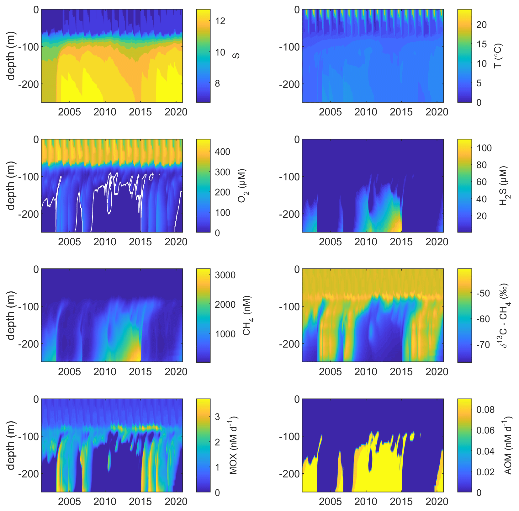
Figure 2Model output from the standard model run, showing simulated S, T (°C), O2 (µM), H2S (µM), CH4 (nM), δ13C–CH4 (‰), MOX (nM d−1), and AOM (nM d−1) in the Gotland Sea sub-basin (cf. Fig. S1) over the period 2001–2020. The white line in the O2 plot indicates the upper limit for anoxic deep water.
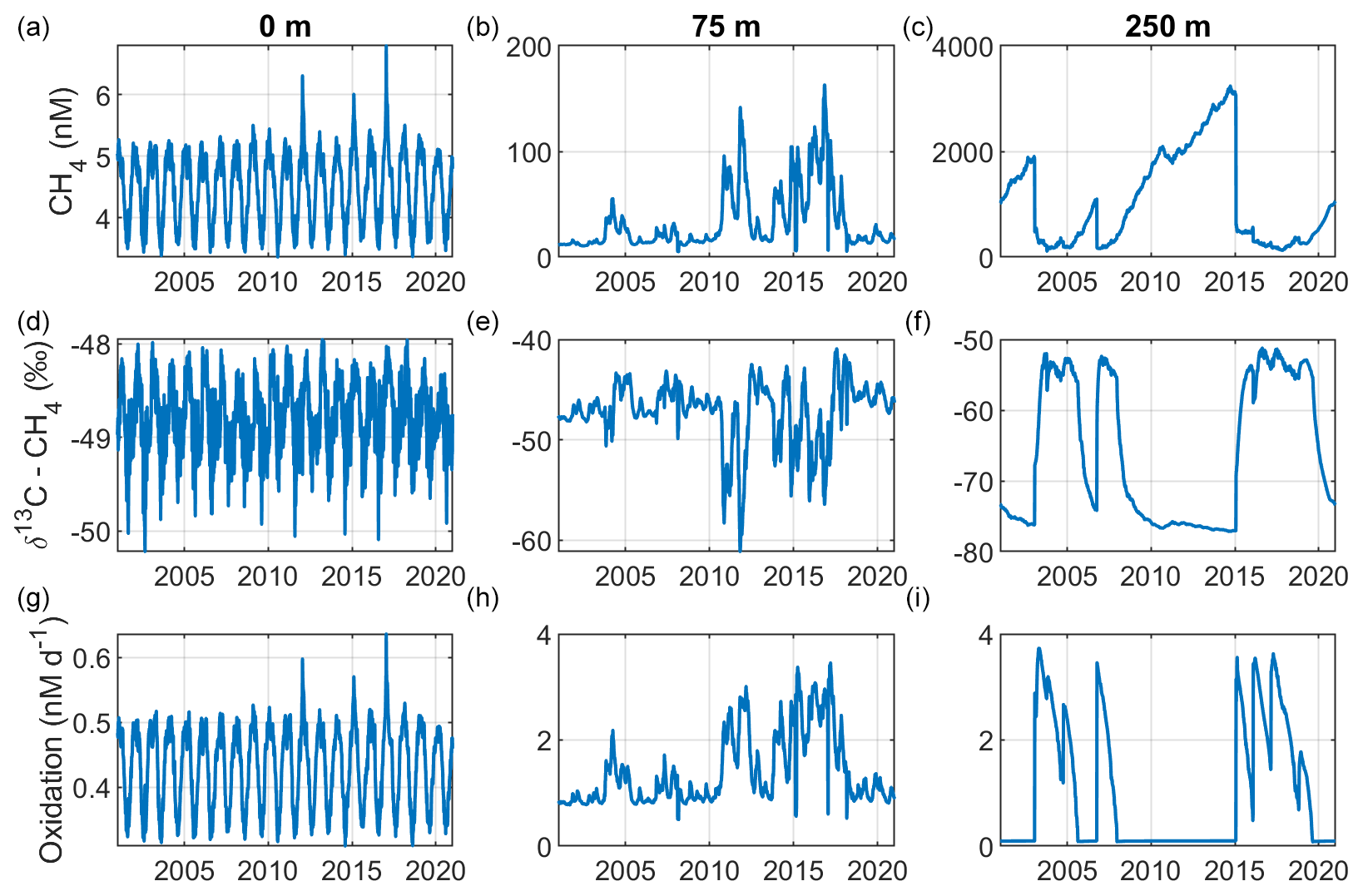
Figure 3Model output from the standard model run, showing simulated surface- (0 m; a, d, g), intermediate- (75 m; b, e, h), and deep-water (250 m; c, f, i) development of CH4 (nM), CH4 oxidation (MOX + AOM; nM d−1), and δ13C–CH4 (‰) in the Gotland Sea sub-basin (cf. Fig. S1) over the period 2001–2020.
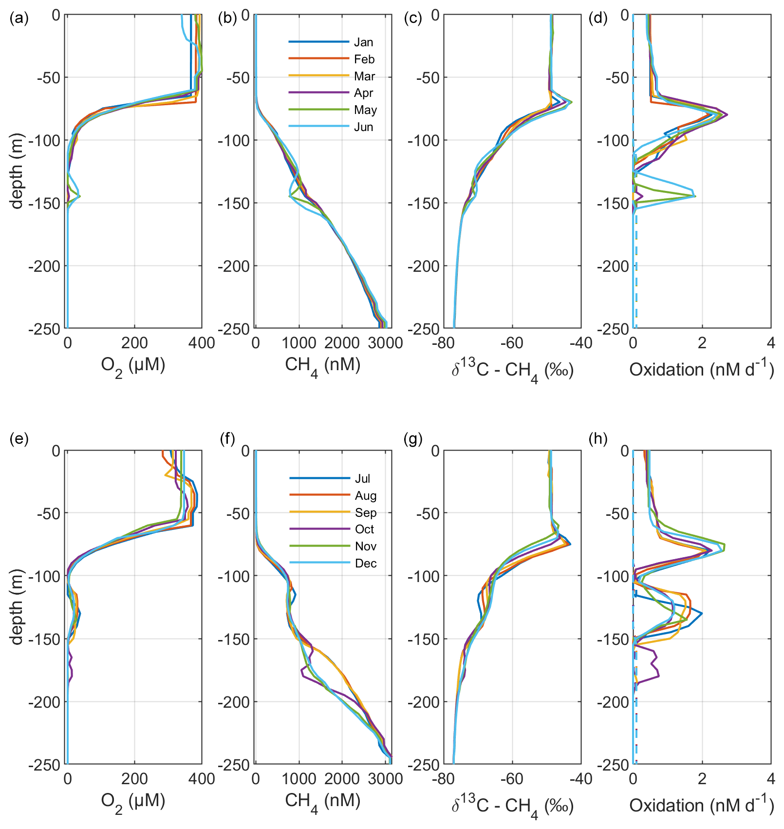
Figure 4Model output from the standard model run, showing simulated monthly mean profiles of CH4 (nM), δ13C–CH4 (‰), and oxidation rates (nM d−1; MOX – full lines, AOM – dashed lines) in the Gotland Sea sub-basin (cf. Fig. S1) for the year 2014. Panels (a)–(d) illustrate monthly mean profiles from January to June; panels (e)–(h) illustrate monthly mean profiles from July to December.
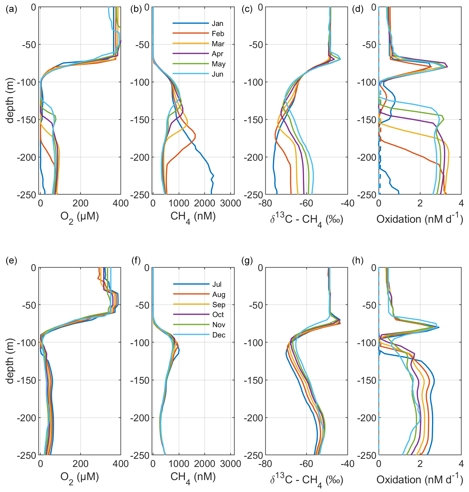
Figure 5Model output from the standard model run, showing simulated monthly mean profiles of CH4 (nM), δ13C–CH4 (‰), and oxidation rates (nM d−1; MOX – full lines, AOM – dashed lines) in the Gotland Sea sub-basin (cf. Fig. S1) for the year 2015. Panels (a)–(d) illustrate monthly mean profiles from January to June; panels (e)–(h) illustrate monthly mean profiles from July to December.
3.1 Standard model run
The standard model run was performed over the period 2001–2020 after spin-up (see Sect. 2.2) with parameters as indicated in Table 1. These parameters (i.e., CH4 oxidation rates and fractionation values; CH4 sources from the sediments, rivers, and the North Sea; and the isotopic compositions of these sources) are mostly fitted values, where the intention was to reproduce reasonably well the existing observations of both CH4 concentration and isotopic composition from the Gotland Sea. This simulation will then be used as a basis for the sensitivity experiments presented in Sect. 4.1. Simulated contour plots and time series for the period 2001–2020 are presented in Figs. 2 and 3. Furthermore, monthly mean profiles for the years 2014 and 2015 are presented in Figs. 4 and 5 in order to illustrate seasonal dynamics in surface waters as well as the impact of a major deep-water inflow.
Table 1Standard model settings. The values are our own estimates/fitted values (see Sect. 2.3) except where noted.
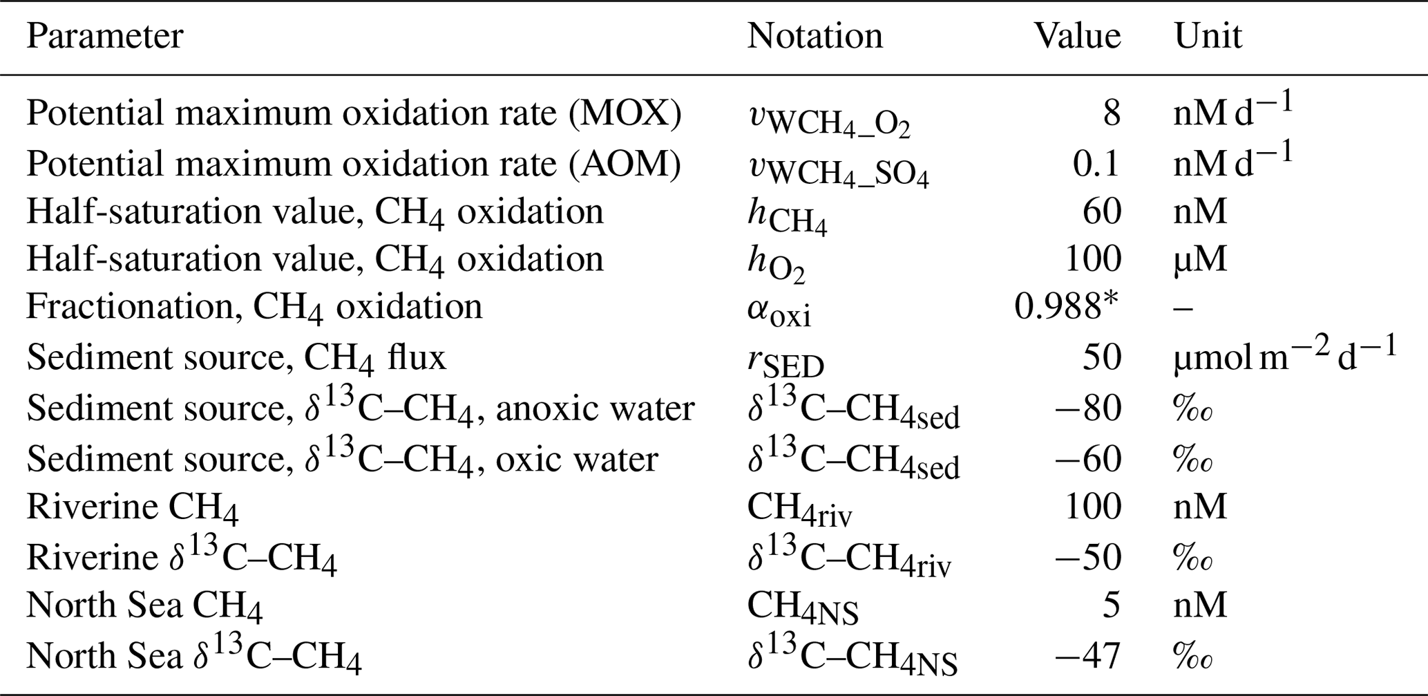
∗ Jakobs et al. (2013)
Figure 2 illustrates the characteristic dynamics of the permanently salinity-stratified Gotland Sea. The top of the halocline, which is typically located at around 60 m depth, isolates deeper waters from the atmosphere, which means that O2 can only be supplied via deep-water inflows of oxic and comparatively high-saline water and through vertical turbulent diffusion. Stagnation periods with little or no advective O2 supply to the deep may last for years, and since O2 consumption by degradation processes exceeds the turbulent diffusive flux, eventually anoxic conditions prevail. Stagnation periods are also characterized by CH4 accumulation because of a low anaerobic oxidation rate, and the δ13C–CH4 in anoxic water is also close to the sediment source because of the marginal influence of anaerobic oxidation processes in the water column. Inflows of new deep water lead to an uplift of the water column above the intrusion depth, which is clearly seen in the simulated O2 and CH4 profiles in February to June of 2015 (Fig. 5, upper panel). Inflows furthermore cause a sharp decline in deep-water CH4 concentration (Figs. 2 and 3), primarily due to water exchange but additionally because of high aerobic oxidation rates during periods when O2 and CH4 co-occur in the deep water until O2 is again depleted (Fig. 5).
In surface waters above the top of the halocline, seasonal changes in temperature and thermal stratification largely influence other parameters (Figs. 4 and 5; see also Figs. S3 and S4 in the Supplement). The increasing surface water temperature in spring and summer leads to decreasing O2 and CH4 solubility, which in addition affects aerobic oxidation rates that depend on O2 and CH4 concentrations (Figs. S3 and S4 in the Supplement; see also Eq. 16). This temperature dependence on oxidation rates also has an impact on the isotopic composition of CH4 – the δ13C–CH4 in water above the top of the halocline is strongly influenced by the seasonality of temperature stratification (Figs. S3 and S4). However, the variations in isotopic composition in surface waters are significantly smaller than the variations at depth where δ13C–CH4 mainly depends on transitions between oxic and anoxic conditions (Figs. 4 and 5).
Observations indicate CH4 concentrations in a range from ∼1000 to 3000 nM in stagnant deep waters of the Baltic Proper (Jakobs et al., 2013; Ketzer et al., 2024) and values below ∼150 nM in oxic deep waters in the same area after a major deep-water intrusion in winter 2014–2015 (Schmale et al., 2016; Myllykangas et al., 2017). These values are well reproduced by the model (Fig. 3) using the settings listed in Table 1, which implies that the simulated sediment CH4 source is likely close to the real source, at least in the deep water where AOM rates are apparently very low (<0.1 nM d−1; Jakobs et al., 2014). The simulated benthic CH4 release from the seafloor amounts to 50 in the standard model run (Table 1), corresponding to ∼18 mmol CH4 m−2 yr−1. This is in the lower range of yearly observations at shallow coastal sites among varying habitats in the Baltic Sea (∼21–34 mmol CH4 m−2 yr−1; Roth et al., 2023).
Measurements from the central Gotland Sea indicate typical surface water CH4 concentrations of 3.5–5 nM, depending on the season (Gülzow et al., 2013), with the highest concentrations observed in winter because of increased gas solubility in cold water. This seasonal cycle is reproduced by the model (Fig. 3). Furthermore, simulated surface water CH4 saturation levels vary between approximately 110 % in winter and 150 % in summer (Fig. S5), which reproduces observed saturation levels (Gülzow et al., 2013).
Measurements from the central Baltic Sea indicate MOX rates ranging from 0.1 to 4 nM d−1 in the redoxcline (Schmale et al., 2012, 2016; Jakobs et al., 2014). In the standard model run, the highest oxidation rates (>3 nM d−1; Fig. 5) occur in the deep water after deep-water intrusions leading to oxygenation of stagnant water with high CH4 concentrations. In the redoxcline, the simulated MOX rates are typically in the range 0.5–3 nM d−1 (Figs. 4–5), which thus matches observed oxidation rates. Simulated surface water MOX rates are in the range 0.3–0.5 nM d−1 (e.g., Fig. 3), whereas observations, on the other hand, indicate rates close to 0 (Jakobs et al., 2014).
Observations indicate a pronounced 13C–CH4 enrichment in the redoxcline. Based on two profiles from 2012, δ13C–CH4 increased from values below −70 ‰ at the bottom of the redoxcline (∼140 m) to −40 ‰ at the top of the redoxcline (∼80 m) in the central Gotland Sea (Jakobs et al., 2014). The δ13C–CH4 peak values at intermediate depths coincide with peak oxidation rates (Jakobs et al., 2014) and result from the preferential oxidation of the lighter isotope. In water above the top of the redoxcline, observations indicate lower oxidation rates and δ13C–CH4 values ranging from −60 ‰ to −40 ‰ depending on the season (Jakobs et al., 2014). In the standard model run, the δ13C–CH4 value typically increases from approximately −70 ‰ at the upper limit for anoxic water (∼130 m) to its peak values between −45 ‰ and −40 ‰ at approximately 75 m (Fig. 4). The simulated δ13C–CH4 in the redoxcline thus tends to be less pronounced than what is apparent from the few available observations. Furthermore, a local minimum of around 30 m observed by Jakobs et al. (2014) is not reproduced in the model run (see further discussion in Sect. 4).
3.2 Preliminary CH4 budget
Here, we present preliminary budget calculations based on the standard model run. It is, however, important to stress that these estimates are heavily dependent on the prescribed benthic CH4 source. As discussed below (Sect. 4), different combinations of benthic CH4 release and MOX rates could produce similar CH4 concentrations in the water column.
To enable a preliminary assessment of the relative importance of different processes, total CH4 sources (river load, import from adjacent sub-basins, and sediment release) and sinks (outgassing, export to adjacent sub-basins, and pelagic oxidation) were aggregated over the Baltic Proper (sub-basins 7–9; Fig. S1), representing the area where the model has been fitted based on available observations. The CH4 sources were largely dominated by benthic release, which amounted to an average 4155 Mmol yr−1 over the period 2001–2020 (Table 2). This source was mainly balanced by oxidation in the water column (3816 Mmol yr−1, 92 % of the sinks) and to a smaller degree by emission to the atmosphere (348 Mmol yr−1, 8 % of the sinks). The river load (11 Mmol yr−1) and net exchange (import – export) with adjacent sub-basins (8 Mmol yr−1) were comparatively small.
Table 2Total CH4 sources, sinks, and net change (= sources − sinks) (Mmol yr−1) aggregated over the Baltic Proper (sub-basins 7–9; Fig. S1) and averaged over the period 2001–2020.
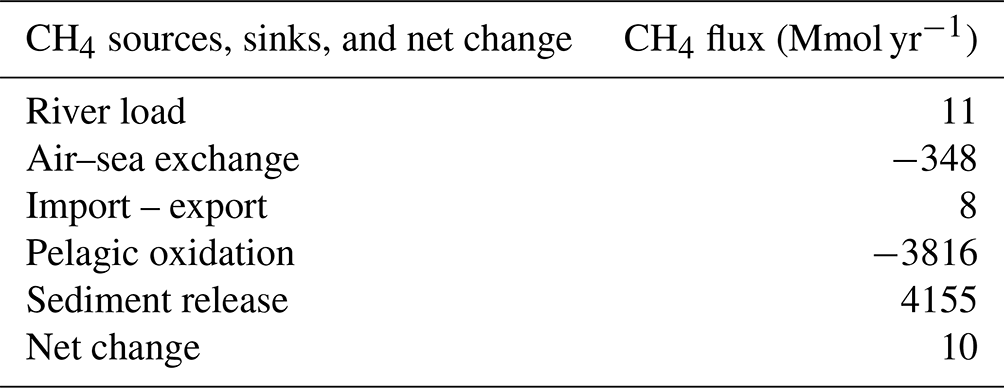
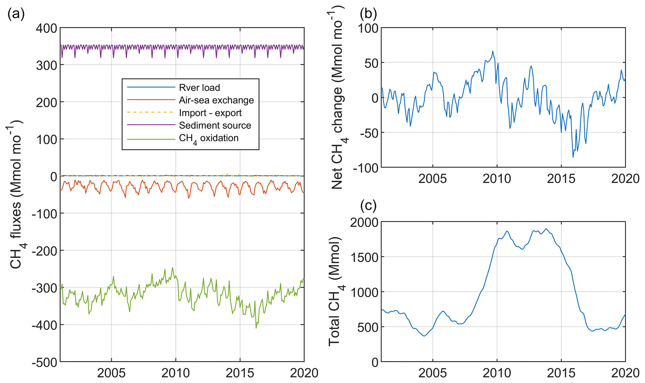
Figure 6Simulated monthly mean CH4 sources and sinks (Mmol mo−1; a), net change (= sources − sinks) (Mmol mo−1; b), and total CH4 stock (Mmol; c) aggregated over the Baltic Proper (sub-basins 7–9; Fig. S1).
Figure 6 illustrates simulated monthly fluxes, net accumulation, and the total amount of CH4 in the Baltic Proper. The total CH4 stock amounted to almost 1800 Mmol over the period ∼2010–2014, which exceeded the stock before and after that period by a factor of 3 (Fig. 6). This comparatively large CH4 stock was the result of a large anoxic deep-water volume and thus of low oxidation rates (Fig. 2). There was an average net accumulation of 10 Mmol yr−1 over the period 2001–2020 (Table 2), but net changes of the total CH4 stock between individual years varied considerably, which largely reflected oxygen-dependent changes in CH4 oxidation rates (Fig. 6).
This study presents a first quantification of key CH4 fluxes in the Baltic Proper. However, there are uncertainties in our estimates, in particular regarding the benthic CH4 source. In the standard model run, benthic release is the dominant CH4 source (Table 2). The sediment source is set as constant over time, at all depths, and in all sub-basins. In the real Baltic Sea, however, large spatial and temporal variations are expected (e.g., Roth et al., 2022). Furthermore, the isotopic composition of the sediment source is set either to −80 ‰ or −60 ‰, depending on oxygen conditions in the overlying water. This assumption is a simplified representation. The main uncertainty in our present large-scale estimates is that spatial and temporal variations in the sediment source are not well known.
The simulated CH4 concentrations in anoxic deep waters agree with the available observations. The fitted rate of CH4 release from sediments is therefore deemed as feasible in anoxic deep waters, since CH4 concentrations are only marginally influenced by oxidation during anoxic conditions (low AOM rates). It is, however, likely that the fitted CH4 release is mainly representative of present-day conditions (e.g., organic carbon deposition rates, oxygen concentrations, temperatures). Both climate change and nutrient load change will affect, e.g., oxygen concentrations in the future, which means that the benthic CH4 source is likely to change as well. In order to address this, it is necessary to improve knowledge of CH4 release rates depending on local conditions. One major uncertainty here is what is the contribution from more recent organic carbon deposition, and what is the contribution from “old” carbon deeper in the sediments, i.e., if nutrient loads and organic carbon deposition decreases, and oxygen conditions improve, would this have a major impact on the CH4 release from sediments, or is the release more heavily dependent on older carbon deposits? This is one of the major open questions remaining regarding CH4 cycling in the Baltic Sea, but it cannot be addressed by the model at this point.
While the fitted flux gives a good idea of the present-day CH4 source in deeper areas, it is more challenging to constrain the sediment source in shallower oxic waters, where the source can be largely compensated by MOX in the water column. Coastal systems are also more dynamic and show a larger variety than deep anoxic areas. A large CH4 source compensated by high MOX rates could, for example, yield similar CH4 concentrations to a smaller source combined with lower MOX rates. These two different cases (i.e., large source, high oxidation vs. small source, low oxidation) would produce quite different isotopic patterns that could be used to calibrate the model. However, a complication here is that we generally do not know the isotopic composition of CH4 released from the sediments, with the exception of observational data from a few locations. Justification of the fitted rates used in the model would require more observational data to fill the knowledge gaps.
Studies from wetlands (Segers, 1998), lakes (Martinez-Cruz et al., 2015; Tan et al., 2015), and oceanic sites (Kessler et al., 2011; Crespo-Medina et al., 2014; Pack et al., 2015; Rogener et al., 2018; Chan et al., 2019a) show that MOX rates can vary by several orders of magnitude. For example, observed deep-water MOX in the Gulf of Mexico increased from a background rate of around 60 pM d−1 to a peak rate of 5900 nM d−1 after the Deepwater Horizon oil spill (Rogener et al., 2018). The observed MOX rates from the central Baltic Sea (approximately 0.1–4 nM d−1; Schmale et al., 2012, 2016; Jakobs et al., 2014) are in the same range as MOX rate observations from the eastern tropical North Pacific Ocean (Pack et al., 2015) but typically lower than MOX rates observed in lakes (Martinez-Cruz et al., 2015; Tan et al., 2015).
In this study, the parameter values used in the computation of MOX rates (Eq. 16) were fitted so that the resulting profiles of oxidation rates and isotopic composition – as well as CH4 concentrations – reproduce the observed profiles from the central Baltic Sea reasonably well. Results for CH4 concentrations, MOX rates, and isotopic composition are sensitive to O2 profiles, which also means that the fitted values depend on how well the model reproduces O2 concentrations.
The rate constant for MOX depends on the activity and abundance of methanotrophs, in theory allowing for reduced MOX in spite of favorable conditions in terms of CH4 and O2 concentrations when methanotrophs are not active. The model does not include methanotrophic activity explicitly, and the rate constant for MOX is constant. Perhaps, lower abundance and activity of methanotrophs could be an explanation for the lower rate constant in the present results compared with the results from lakes cited above.
The present study does not include the potential contributions from aerobic CH4 production. There are, however, several potential pathways for CH4 production in shallow oxic waters, including, e.g., direct CH4 production by phytoplankton (Lenhart et al., 2016) and cyanobacteria (Bižić et al., 2020), CH4 production as a byproduct of microbial degradation processes (Karl et al., 2008; Damm et al., 2010), and CH4 formation in anoxic microniches within degrading detritus (Karl and Tilbrook, 1994; Holmes et al., 2000). In the Baltic Sea, local CH4 maxima coinciding with δ13C–CH4 minima have been observed in oxic waters just below the summer thermocline (Jakobs et al., 2014; Schmale et al., 2018). These signals can be coupled with zooplankton grazing activities, both directly through CH4 production during digestion and indirectly via release of methanogenic substrates that can subsequently be degraded to methane by microbes (Schmale et al., 2018; Stawiarski et al., 2019). However, the main pathways as well as the magnitude of aerobic CH4 production in the Baltic Sea remain to be resolved in detail. Parameterizations of these processes can then potentially be included in models such as BALTSEM that explicitly include both phytoplankton and zooplankton groups as model state variables.
4.1 Sensitivity experiments
A series of sensitivity experiments were performed on different parameters used in the modeling of CH4 and its stable isotopes (Table 1). The adjusted parameter values are listed in Table 3. Modeled profiles are then drawn for both winter conditions (February) and summer conditions (August) of 2015 (Figs. S6–S11), which gives an indication of season-dependent contrasting conditions in surface waters above the halocline. Methane cycling in the model is largely dominated by benthic release, oxidation in the water column, and outgassing (Table 2; Fig. 6). For that reason, sensitivity experiments on riverine and North Sea CH4 concentrations were not included.
Table 3Adjusted parameter values and change (%) compared with the standard model run in the various sensitivity experiments.
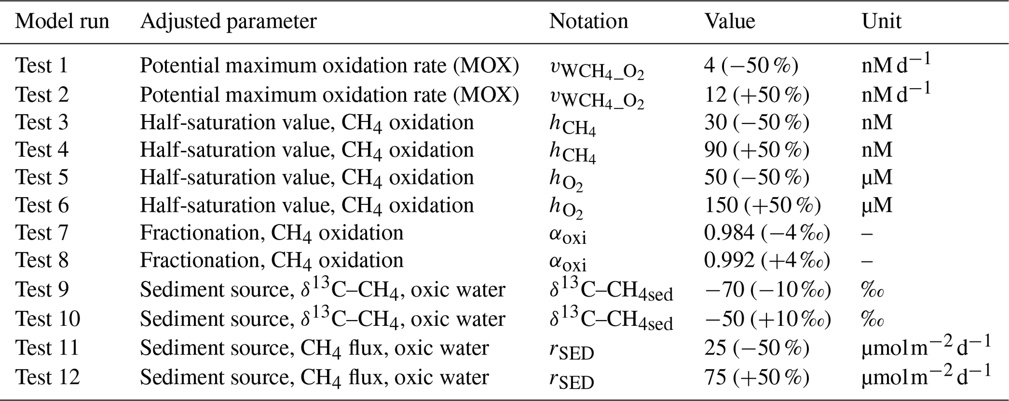
4.1.1 MOX and AOM: rates, half-saturation constants, and fractionation
Adjusting the potential maximum rate of MOX () by ±50 % (tests 1 and 2) has a large influence on CH4 concentrations (Fig. S6), where decreased (test 1) leads to substantially higher CH4 concentrations, and increased (test 2) leads to lower CH4 compared with the standard model run. Since the MOX rate in addition to depends on CH4 concentration, the changed CH4 concentration in itself will further modify the shape of the MOX profile (CH4 oxidation also consumes O2, but the influence on O2 concentration is small compared with the influence on CH4 concentration, since O2 and CH4 typically differ by orders of magnitude). The modified shapes of the MOX profiles also influence the δ13C–CH4 profiles, with changed depths of the intermediate deep-water peak as well as changed peak values. Adjusting the potential maximum rate of AOM () has a comparatively minor influence on both the CH4 concentration and the isotopic composition because of the low anaerobic oxidation rates (not shown).
Adjusting the half-saturation values for CH4 oxidation ( and ) by ±50 % (tests 3–6) influences the MOX rates and thus both the CH4 concentration and the isotopic composition (Figs. S7 and S8). These parameters alter the dynamics within a relatively small range close to their respective values. Thus, the MOX rate is most sensitive to changes of where the CH4 concentration is close to 60 nM and, similarly, most sensitive to changes of where the O2 concentration is close to 100 µM (Table 1). At high concentrations compared with the values of and , we do not expect a large impact by adjusting these constants. On the other hand, at low concentrations compared with the constants, the sensitivity to changed values of and is expected to be similar to changing the potential maximum rate constant ().
In these particular experiments, CH4 dynamics is more sensitive to changes in than , and the reason for this is the relatively large water volume where the O2 concentration is close to , while the CH4 concentration, on the other hand, is only close to in a comparatively narrow band at intermediate depths. The modified CH4 dynamics is, however, transferred to other depths by turbulent diffusion and vertical internal circulation (“old” water mixing into the intruding new deep water), which means that altered CH4 concentrations, δ values, and MOX rates are (more or less) apparent throughout the entire water column.
Adjusting the fractionation during CH4 oxidation by ±4 ‰ (tests 7 and 8) has no influence on CH4 oxidation rates and concentrations but a relatively strong (and predictable) impact on δ13C–CH4 values throughout the entire water column (Fig. S9).
4.1.2 Sediment source: CH4 release and isotopic composition
As indicated in Sect. 4, it is expected that the isotopic composition of the sediment source differs between different locations depending on the degree of oxidation in the pore water. The rate of CH4 release is also expected to depend on the balance between benthic CH4 production and oxidation. Adjusting the δ13C–CH4 value of the sediment source by ±10 ‰ during oxic conditions (tests 9 and 10) has no influence on CH4 oxidation rates and concentrations but a strong (and predictable) impact on δ13C–CH4 profiles (Fig. S10).
In experiments where the rate of CH4 release from the sediments source was adjusted by ±50 ‰ during oxic conditions (tests 11 and 12), strong impacts are apparent for both the CH4 concentration and isotopic composition throughout the water column. Deep-water MOX rates are, however, less sensitive, since the rates in these cases depend more on O2 concentration – which is very similar between the two experiments (not shown) – than on CH4 concentrations (Fig. S11).
4.2 Caveats and outlook
As previously discussed, the main uncertainty in the model simulations lies in our limited understanding of CH4 release from different sediment areas as well as in the isotopic composition of CH4 released into the water column. Both the flux and the isotopic composition depend on the balance between production and oxidation rates in the sediment. A high production could be compensated by high oxidation and thus result in a relatively small CH4 release to the water column in spite of a large production. This would then be evident by a 13C–CH4 enrichment, i.e., comparatively heavy CH4. Alternatively, a relatively small CH4 production could still result in a substantial release to the water column in the case where the oxidation rate is low, which would then also be evident by CH4 depleted in 13C–CH4, i.e., comparatively light CH4.
Improved knowledge of properties of CH4 released from the sediment to the water column in different areas of the Baltic Sea (e.g., the Kattegat and the major gulfs – the Gulf of Bothnia, Gulf of Riga, and Gulf of Finland) would help to improve model parameterizations and thus reduce the main uncertainties of model simulations. This was, however, beyond the scope of the present study because of the missing knowledge concerning both temporal and spatial patterns of the CH4 source. A logical progression at this stage would involve detailed observations combined with modeling studies focused on processes in the sediments, i.e., production and oxidation rates, depending on the carbon accumulation rate, oxygen conditions, and the presence of methanotrophs.
A crucial missing link in this study is the formation, transport, and fate of CH4 bubbles. Estimates by Weber et al. (2019) indicate that ebullitive fluxes contribute a major fraction of CH4 released to the atmosphere from shallow coastal areas. Ebullition events have been observed in the Baltic Sea, both at coastal sites (e.g., Humborg et al., 2019; Lohrberg et al., 2020; Lehoux et al., 2021; Hermans et al., 2024) and deep-water accumulation bottoms (Christian Stranne, unpublished data). Ebullition has been included in lake models (e.g., Greene et al., 2014; Stepanenko et al., 2016; Bayer et al., 2019); however, we do not have experimental data to calibrate and validate the large-scale influence of ebullition in the Baltic Sea. The fitted benthic CH4 source represents a “bulk” CH4 release, including in theory both the influences of diffusive flux and bubble dissolution on CH4 concentrations in the water column. However, CH4 ebullition might bypass methanotrophy and consequently contribute to higher CH4 emissions, in particular in shallow-water areas (e.g., Broman et al., 2020). This indicates that the simulated CH4 outgassing is likely underestimating the real outgassing from the Baltic Sea. Observations of ebullitive fluxes in combination with the development of model parameterizations represent important steps to better describe and quantify CH4 emissions from the Baltic Sea. When it comes to local production of gas bubbles and the transformation and fate of methane in the bubbles, the horizontally averaged approach used in the present study is most likely insufficient, which could be addressed either by 3D modeling or by adding smaller sub-domains to the present model.
Roth et al. (2023) observed significant CH4 production and release from vegetated oxic shallow-water areas. BALTSEM-CH4 v1.0 does not differentiate between vegetated and unvegetated areas, which means that this CH4 source – and its contribution to outgassing – could not be addressed here, which consequently represents another gap in our current understanding. Both species distribution models and process-based models for vegetation exist (e.g., Lappalainen et al., 2019; Graiff et al., 2020), but to our knowledge they do not include CH4 dynamics. Hence, the inclusion of CH4 in vegetation models could be an objective for future scientific projects.
The process parameterizations used in this study to describe large-scale CH4 cycling in the Baltic Sea can also be applied in various other domains. As part of our future plans, we aim to investigate CH4 dynamics in a smaller area where more observations are available and where the CH4 concentration and isotopic composition, as well as properties of end-members (river load, benthic release, and lateral boundary conditions), are better understood. This would further help to constrain process rates in the model.
The calculated average total CH4 emission of 348 Mmol yr−1 from the Baltic Proper corresponds to approximately 1.5 mmol CH4 m−2 yr−1 and constitutes only about 8 % of the fitted sediment source (∼18 mmol CH4 m−2 yr−1). The model includes both shallow- and deep-water sediment areas, but the fitted sediment source is in the lower range of rates reported for a shallow-water coastal area (∼21–34 mmol CH4 m−2 yr−1; Roth et al., 2023), indicating that the model might not well represent coastal CH4 hotspots. One major knowledge gap at this point is the relative importance of shallow coastal areas compared with the open Baltic Sea in terms of CH4 outgassing. This is an important scientific question that needs to be addressed in future studies.
Table A1Pelagic and sediment state variables in BALTSEM-CH4 v1.0.
Model forcing consists of actual weather data and observed nutrient loads as well as calibrated carbon and total alkalinity loads (Gustafsson and Gustafsson, 2020) covering the period 1970–2020. River runoff, land loads, and atmospheric depositions were based on Pollution Load Compilation data (PLC; HELCOM, 2021) as well as other sources (Gustafsson et al., 2012). Atmospheric forcing was constructed from data provided by the Swedish Meteorological and Hydrological Institute (SMHI): RCA-ERA40 (1970–2006), Hirlam-Mesan (2007–2015), and Arome-Mesan (2016–2020). The Kattegat water level and the boundary conditions in the Skagerrak were based on data provided by the SMHI (Gustafsson et al., 2012).
All model output data for the standard model run as well as the version of the model source code used in this study are archived on Zenodo at https://doi.org/10.5281/zenodo.10037197 (Gustafsson and Gustafsson, 2023). In addition to the model output and source code, the archive includes initial profiles, boundary conditions, meteorological forcing, and runoff as well as river loads, point sources, and atmospheric depositions of dissolved and particulate constituents.
The supplement related to this article is available online at: https://doi.org/10.5194/gmd-17-7157-2024-supplement.
EG wrote the first draft of the manuscript with contributions from all co-authors. EG developed the CH4 model components and designed and performed the model experiments and analyses. BGG is the main developer of the BALTSEM model.
The contact author has declared that none of the authors has any competing interests.
Publisher's note: Copernicus Publications remains neutral with regard to jurisdictional claims made in the text, published maps, institutional affiliations, or any other geographical representation in this paper. While Copernicus Publications makes every effort to include appropriate place names, the final responsibility lies with the authors.
This research is part of the University of Helsinki and Stockholm University collaborative research initiative (CoastClim, http://www.coastclim.org, last access: 23 September 2024; the Baltic Bridge initiative). Financial support was provided by the Swedish Research Council (VR; grant no. 2021-04641).
This research has been supported by the Havs- och Vattenmyndigheten (grant no. 1:11 – Measures for marine and water environment).
The publication of this article was funded by the Swedish Research Council, Forte, Formas, and Vinnova.
This paper was edited by Andrew Yool and reviewed by two anonymous referees.
Asplund, M. E., Bonaglia, S., Boström, C., Dahl, M., Deyanova, D., Gagnon, K., Gullström, M., Holmer, M., and Björk, M.: Methane Emissions From Nordic Seagrass Meadow Sediments, Front. Mar. Sci., 8, 811533, https://doi.org/10.3389/fmars.2021.811533, 2022.
Atkins, M. L., Santos, I. R., and Maher, D. T.: Seasonal exports and drivers of dissolved inorganic and organic carbon, carbon dioxide, methane and δ13C signatures in a subtropical river network, Sci. Total Environ., 575, 545–563, https://doi.org/10.1016/j.scitotenv.2016.09.020, 2017.
Axell, L. B.: On the variability of Baltic Sea deepwater mixing, J. Geophys. Res.-Oceans, 103, 21667–21682, https://doi.org/10.1029/98JC01714, 1998.
Bange, H. W., Bartell, U. H., Rapsomanikis, S., and Andreae, M. O.: Methane in the Baltic and North Seas and a reassessment of the marine emissions of methane, Global Biogeochem. Cycles, 8, 465–480, https://doi.org/10.1029/94GB02181, 1994.
Bayer, T. K., Gustafsson, E., Brakebusch, M., and Beer, C.: Future Carbon Emission From Boreal and Permafrost Lakes Are Sensitive to Catchment Organic Carbon Loads, J. Geophys. Res.-Biogeo., 124, 1827–1848, https://doi.org/10.1029/2018JG004978, 2019.
Bižić, M., Klintzsch, T., Ionescu, D., Hindiyeh, M. Y., Günthel, M., Muro-Pastor, A. M., Eckert, W., Urich, T., Keppler, F., and Grossart, H.-P.: Aquatic and terrestrial cyanobacteria produce methane, Sci. Adv., 6, eaax5343, https://doi.org/10.1126/sciadv.aax5343, 2020.
Björk, G.: The relation between ice deformation, oceanic heat flux, and the ice thickness distribution in the Arctic Ocean, J. Geophys. Res.-Oceans, 102, 18681–18698, https://doi.org/10.1029/97JC00789, 1997.
Borges, A. V., Champenois, W., Gypens, N., Delille, B., and Harlay, J.: Massive marine methane emissions from near-shore shallow coastal areas, Sci. Rep., 6, 27908, https://doi.org/10.1038/srep27908, 2016.
Broman, E., Sun, X., Stranne, C., Salgado, M. G., Bonaglia, S., Geibel, M., Jakobsson, M., Norkko, A., Humborg, C., and Nascimento, F. J. A.: Low Abundance of Methanotrophs in Sediments of Shallow Boreal Coastal Zones With High Water Methane Concentrations, Front. Microbiol., 11, 1536, https://doi.org/10.3389/fmicb.2020.01536, 2020.
Carstensen, J., Andersen, J. H., Gustafsson, B. G., and Conley, D. J.: Deoxygenation of the Baltic Sea during the last century, P. Natl. Acad. Sci. USA, 111, 5628–5633, https://doi.org/10.1073/pnas.1323156111, 2014.
Chan, E. W., Shiller, A. M., Joung, D. J., Arrington, E. C., Valentine, D. L., Redmond, M. C., Breier, J. A., Socolofsky, S. A., and Kessler, J. D.: Investigations of Aerobic Methane Oxidation in Two Marine Seep Environments: Part 1 – Chemical Kinetics, J. Geophys. Res.-Oceans, 124, 8852–8868, https://doi.org/10.1029/2019JC015594, 2019a.
Chan, E. W., Shiller, A. M., Joung, D. J., Arrington, E. C., Valentine, D. L., Redmond, M. C., Breier, J. A., Socolofsky, S. A., and Kessler, J. D.: Investigations of Aerobic Methane Oxidation in Two Marine Seep Environments: Part 2 – Isotopic Kinetics, J. Geophys. Res.-Oceans, 124, 8392–8399, https://doi.org/10.1029/2019JC015603, 2019b.
Chuang, P.-C., Yang, T. F., Wallmann, K., Matsumoto, R., Hu, C.-Y., Chen, H.-W., Lin, S., Sun, C.-H., Li, H.-C., Wang, Y., and Dale, A. W.: Carbon isotope exchange during anaerobic oxidation of methane (AOM) in sediments of the northeastern South China Sea, Geochim. Cosmochim. Ac., 246, 138–155, https://doi.org/10.1016/j.gca.2018.11.003, 2019.
Crespo-Medina, M., Meile, C. D., Hunter, K. S., Diercks, A.-R., Asper, V. L., Orphan, V. J., Tavormina, P. L., Nigro, L. M., Battles, J. J., Chanton, J. P., Shiller, A. M., Joung, D.-J., Amon, R. M. W., Bracco, A., Montoya, J. P., Villareal, T. A., Wood, A. M., and Joye, S. B.: The rise and fall of methanotrophy following a deepwater oil-well blowout, Nat. Geosci., 7, 423–427, https://doi.org/10.1038/ngeo2156, 2014.
Damm, E., Helmke, E., Thoms, S., Schauer, U., Nöthig, E., Bakker, K., and Kiene, R. P.: Methane production in aerobic oligotrophic surface water in the central Arctic Ocean, Biogeosciences, 7, 1099–1108, https://doi.org/10.5194/bg-7-1099-2010, 2010.
Dickson, A. G., Sabine, C. L., and Christian, J. R. (Eds.): Guide to best practices for ocean CO2 measurements. PICES Special Publication 3, North Pacific Marine Science Organization, Sidney, BC, 191 pp., 2007.
Egger, M., Hagens, M., Sapart, C. J., Dijkstra, N., van Helmond, N. A. G. M., Mogollón, J. M., Risgaard-Petersen, N., van der Veen, C., Kasten, S., Riedinger, N., Böttcher, M. E., Röckmann, T., Jørgensen, B. B., and Slomp, C. P.: Iron oxide reduction in methane-rich deep Baltic Sea sediments, Geochim. Cosmochim. Ac., 207, 256–276, https://doi.org/10.1016/j.gca.2017.03.019, 2017.
Etminan, M., Myhre, G., Highwood, E. J., and Shine, K. P.: Radiative forcing of carbon dioxide, methane, and nitrous oxide: A significant revision of the methane radiative forcing, Geophys. Res. Lett., 43, 12614–12623, https://doi.org/10.1002/2016GL071930, 2016.
Ferretti, D. F., Miller, J. B., White, J. W. C., Etheridge, D. M., Lassey, K. R., Lowe, D. C., Meure, C. M. M., Dreier, M. F., Trudinger, C. M., van Ommen, T. D., and Langenfelds, R. L.: Unexpected Changes to the Global Methane Budget over the Past 2000 Years, Science, 309, 1714–1717, https://doi.org/10.1126/science.1115193, 2005.
Fuex, A. N.: Experimental evidence against an appreciable isotopic fractionation of methane during migration, Phys. Chem. Earth, 12, 725–732, https://doi.org/10.1016/0079-1946(79)90153-8, 1980.
Graiff, A., Karsten, U., Radtke, H., Wahl, M., and Eggert, A.: Model simulation of seasonal growth of Fucus vesiculosus in its benthic community, Limnol. Oceanogr.-Methods, 18, 89–115, https://doi.org/10.1002/lom3.10351, 2020.
Greene, S., Walter Anthony, K. M., Archer, D., Sepulveda-Jauregui, A., and Martinez-Cruz, K.: Modeling the impediment of methane ebullition bubbles by seasonal lake ice, Biogeosciences, 11, 6791–6811, https://doi.org/10.5194/bg-11-6791-2014, 2014.
Grunwald, M., Dellwig, O., Beck, M., Dippner, J. W., Freund, J. A., Kohlmeier, C., Schnetger, B., and Brumsack, H.-J.: Methane in the southern North Sea: Sources, spatial distribution and budgets, Estuarine, Coast. Shelf Sci., 81, 445–456, https://doi.org/10.1016/j.ecss.2008.11.021, 2009.
Gu, C., Waldron, S., and Bass, A. M.: Carbon dioxide, methane, and dissolved carbon dynamics in an urbanized river system, Hydrol. Process., 35, e14360, https://doi.org/10.1002/hyp.14360, 2021.
Gustafsson, B.: A time-dependent coupled-basin model for the Baltic Sea, C47, Göteborg: Earth Sciences Centre, Göteborg University, 2003.
Gustafsson, B. and Gustafsson, E.: BALTSEM with methane model and sample outputs, Baltsem9.5_CH4, Zenodo [code and data set], https://doi.org/10.5281/zenodo.10037197, 2023.
Gustafsson, B. G.: Time-dependent modeling of the Baltic entrance area. 1. Quantification of circulation and residence times in the Kattegat and the Straits of the Baltic sill, Estuaries, 23, 231–252, https://doi.org/10.2307/1352830, 2000.
Gustafsson, B. G., Schenk, F., Blenckner, T., Eilola, K., Meier, H. E. M., Müller-Karulis, B., Neumann, T., Ruoho-Airola, T., Savchuk, O. P., and Zorita, E.: Reconstructing the Development of Baltic Sea Eutrophication 1850–2006, AMBIO, 41, 534–548, https://doi.org/10.1007/s13280-012-0318-x, 2012.
Gustafsson, E. and Gustafsson, B. G.: Future acidification of the Baltic Sea – A sensitivity study, J. Marine Syst., 211, 103397, https://doi.org/10.1016/j.jmarsys.2020.103397, 2020.
Gustafsson, E., Deutsch, B., Gustafsson, B. G., Humborg, C., and Mörth, C.-M.: Carbon cycling in the Baltic Sea – The fate of allochthonous organic carbon and its impact on air–sea CO2 exchange, J. Marine Syst., 129, 289–302, https://doi.org/10.1016/j.jmarsys.2013.07.005, 2014.
Gustafsson, E., Mörth, C.-M., Humborg, C., and Gustafsson, B. G.: Modelling the 13C and 12C isotopes of inorganic and organic carbon in the Baltic Sea, J. Marine Syst., 148, 122–130, https://doi.org/10.1016/j.jmarsys.2015.02.008, 2015.
Gustafsson, E., Savchuk, O. P., Gustafsson, B. G., and Müller-Karulis, B.: Key processes in the coupled carbon, nitrogen, and phosphorus cycling of the Baltic Sea, Biogeochemistry, 134, 301–317, https://doi.org/10.1007/s10533-017-0361-6, 2017.
Gülzow, W., Rehder, G., Schneider v. Deimling, J., Seifert, T., and Tóth, Z.: One year of continuous measurements constraining methane emissions from the Baltic Sea to the atmosphere using a ship of opportunity, Biogeosciences, 10, 81–99, https://doi.org/10.5194/bg-10-81-2013, 2013.
Gülzow, W., Gräwe, U., Kedzior, S., Schmale, O., and Rehder, G.: Seasonal variation of methane in the water column of Arkona and Bornholm Basin, western Baltic Sea, J. Marine Syst., 139, 332–347, https://doi.org/10.1016/j.jmarsys.2014.07.013, 2014.
Hansson, M. and Viktorsson, L.: Oxygen Survey in the Baltic Sea 2022 – Extent of Anoxia and Hypoxia, 1960–2022, SMHI, Göteborg, 2023.
Happell, J. D., Chanton, J. P., and Showers, W. J.: Methane transfer across the water-air interface in stagnant wooded swamps of Florida: Evaluation of mass-transfer coefficients and isotropic fractionation, Limnol. Oceanogr., 40, 290–298, https://doi.org/10.4319/lo.1995.40.2.0290, 1995.
HELCOM: HELCOM Baltic Sea Action Plan – 2021 update, http://helcom.fi (last access: 23 September 2024), 2021.
Hermans, M., Stranne, C., Broman, E., Sokolov, A., Roth, F., Nascimento, F. J. A., Mörth, C.-M., ten Hietbrink, S., Sun, X., Gustafsson, E., Gustafsson, B. G., Norkko, A., Jilbert, T., and Humborg, C.: Ebullition dominates methane emissions in stratified coastal waters, Sci. Total Environ., 945, 174183, https://doi.org/10.1016/j.scitotenv.2024.174183, 2024.
Hoehler, T. M., Alperin, M. J., Albert, D. B., and Martens, C. S.: Field and laboratory studies of methane oxidation in an anoxic marine sediment: Evidence for a methanogen-sulfate reducer consortium, Global Biogeochem. Cycles, 8, 451–463, https://doi.org/10.1029/94GB01800, 1994.
Hoffman, D. W. and Rasmussen, C.: Absolute Carbon Stable Isotope Ratio in the Vienna Peedee Belemnite Isotope Reference Determined by 1H NMR Spectroscopy, Anal. Chem., 94, 5240–5247, https://doi.org/10.1021/acs.analchem.1c04565, 2022.
Holmes, M. E., Sansone, F. J., Rust, T. M., and Popp, B. N.: Methane production, consumption, and air-sea exchange in the open ocean: An Evaluation based on carbon isotopic ratios, Global Biogeochem. Cycles, 14, 1–10, https://doi.org/10.1029/1999GB001209, 2000.
Humborg, C., Geibel, Marc. C., Sun, X., McCrackin, M., Mörth, C.-M., Stranne, C., Jakobsson, M., Gustafsson, B., Sokolov, A., Norkko, A., and Norkko, J.: High Emissions of Carbon Dioxide and Methane From the Coastal Baltic Sea at the End of a Summer Heat Wave, Front. Marine Sci., 6, 493, https://doi.org/10.3389/fmars.2019.00493, 2019.
Jakobs, G., Rehder, G., Jost, G., Kießlich, K., Labrenz, M., and Schmale, O.: Comparative studies of pelagic microbial methane oxidation within the redox zones of the Gotland Deep and Landsort Deep (central Baltic Sea), Biogeosciences, 10, 7863–7875, https://doi.org/10.5194/bg-10-7863-2013, 2013.
Jakobs, G., Holtermann, P., Berndmeyer, C., Rehder, G., Blumenberg, M., Jost, G., Nausch, G., and Schmale, O.: Seasonal and spatial methane dynamics in the water column of the central Baltic Sea (Gotland Sea), Cont. Shelf Res., 91, 12–25, https://doi.org/10.1016/j.csr.2014.07.005, 2014.
Jørgensen, B. B., Bang, M., and Blackburn, T.: Anaerobic mineralization in marine sediments from the Baltic Sea-North Sea transition, Marine Ecol. Prog. Ser., 59, 39–54, 1990.
Karl, D. M. and Tilbrook, B. D.: Production and transport of methane in oceanic particulate organic matter, Nature, 368, 732–734, https://doi.org/10.1038/368732a0, 1994.
Karl, D. M., Beversdorf, L., Björkman, K. M., Church, M. J., Martinez, A., and Delong, E. F.: Aerobic production of methane in the sea, Nat. Geosci., 1, 473–478, https://doi.org/10.1038/ngeo234, 2008.
Kessler, J. D., Valentine, D. L., Redmond, M. C., Du, M., Chan, E. W., Mendes, S. D., Quiroz, E. W., Villanueva, C. J., Shusta, S. S., Werra, L. M., Yvon-Lewis, S. A., and Weber, T. C.: A Persistent Oxygen Anomaly Reveals the Fate of Spilled Methane in the Deep Gulf of Mexico, Science, 331, 312–315, https://doi.org/10.1126/science.1199697, 2011.
Ketzer, M., Stranne, C., Rahmati-Abkenar, M., Shahabi-Ghahfarokhi, S., Jaeger, L., Pivel, M. A. G., Josefsson, S., and Zillén, L.: Near seafloor methane flux in the world's largest human-induced dead zone is regulated by sediment accumulation rate, Marine Geol., 468, 107220, https://doi.org/10.1016/j.margeo.2024.107220, 2024.
Knox, M., Quay, P. D., and Wilbur, D.: Kinetic isotopic fractionation during air-water gas transfer of O2, N2, CH4, and H2, J. Geophys. Res.-Oceans, 97, 20335–20343, https://doi.org/10.1029/92JC00949, 1992.
Kremling, K.: Untersuchungen Über die chemische Zusammensetzung des Meerwassers aus der Ostsee, III. Früjahr 1969–Herbst 1970, Kiel. Meeresforsch., 28, 99–118, https://oceanrep.geomar.de/id/eprint/54305/ (last access: 23 September 2024), 1972.
Kuliński, K., Rehder, G., Asmala, E., Bartosova, A., Carstensen, J., Gustafsson, B., Hall, P. O. J., Humborg, C., Jilbert, T., Jürgens, K., Meier, H. E. M., Müller-Karulis, B., Naumann, M., Olesen, J. E., Savchuk, O., Schramm, A., Slomp, C. P., Sofiev, M., Sobek, A., Szymczycha, B., and Undeman, E.: Biogeochemical functioning of the Baltic Sea, Earth Syst. Dynam., 13, 633–685, https://doi.org/10.5194/esd-13-633-2022, 2022.
Lan, X., Basu, S., Schwietzke, S., Bruhwiler, L. M. P., Dlugokencky, E. J., Michel, S. E., Sherwood, O. A., Tans, P. P., Thoning, K., Etiope, G., Zhuang, Q., Liu, L., Oh, Y., Miller, J. B., Pétron, G., Vaughn, B. H., and Crippa, M.: Improved Constraints on Global Methane Emissions and Sinks Using δ13C-CH4, Global Biogeochem. Cycles, 35, e2021GB007000, https://doi.org/10.1029/2021GB007000, 2021.
Lappalainen, J., Virtanen, E. A., Kallio, K., Junttila, S., and Viitasalo, M.: Substrate limitation of a habitat-forming genus Fucus under different water clarity scenarios in the northern Baltic Sea, Estuar. Coast. Shelf Sci., 218, 31–38, https://doi.org/10.1016/j.ecss.2018.11.010, 2019.
Lehoux, A. P., Isidorova, A., Collin, F., Koestel, J., Snowball, I., and Dahlberg, A.-K.: Extreme gas production in anthropogenic fibrous sediments: An overlooked biogenic source of greenhouse gas emissions, Sci. Total Environ., 781, 146772, https://doi.org/10.1016/j.scitotenv.2021.146772, 2021.
Lenhart, K., Klintzsch, T., Langer, G., Nehrke, G., Bunge, M., Schnell, S., and Keppler, F.: Evidence for methane production by the marine algae Emiliania huxleyi, Biogeosciences, 13, 3163–3174, https://doi.org/10.5194/bg-13-3163-2016, 2016.
Lohrberg, A., Schmale, O., Ostrovsky, I., Niemann, H., Held, P., and Schneider von Deimling, J.: Discovery and quantification of a widespread methane ebullition event in a coastal inlet (Baltic Sea) using a novel sonar strategy, Sci. Rep., 10, 4393, https://doi.org/10.1038/s41598-020-60283-0, 2020.
Lopes, F., Viollier, E., Thiam, A., Michard, G., Abril, G., Groleau, A., Prévot, F., Carrias, J.-F., Albéric, P., and Jézéquel, D.: Biogeochemical modelling of anaerobic vs. aerobic methane oxidation in a meromictic crater lake (Lake Pavin, France), Appl. Geochem., 26, 1919–1932, https://doi.org/10.1016/j.apgeochem.2011.06.021, 2011.
Lundevall-Zara, M., Lundevall-Zara, E., and Brüchert, V.: Sea-Air Exchange of Methane in Shallow Inshore Areas of the Baltic Sea, Front. Marine Sci., 8, 657459, https://doi.org/10.3389/fmars.2021.657459, 2021.
Malakhova, V. and Golubeva, E.: Model Study of the Effects of Climate Change on the Methane Emissions on the Arctic Shelves, Atmosphere, 13, 274, https://doi.org/10.3390/atmos13020274, 2022.
Martinez-Cruz, K., Sepulveda-Jauregui, A., Walter Anthony, K., and Thalasso, F.: Geographic and seasonal variation of dissolved methane and aerobic methane oxidation in Alaskan lakes, Biogeosciences, 12, 4595–4606, https://doi.org/10.5194/bg-12-4595-2015, 2015.
Myllykangas, J.-P., Jilbert, T., Jakobs, G., Rehder, G., Werner, J., and Hietanen, S.: Effects of the 2014 major Baltic inflow on methane and nitrous oxide dynamics in the water column of the central Baltic Sea, Earth Syst. Dynam., 8, 817–826, https://doi.org/10.5194/esd-8-817-2017, 2017.
Myllykangas, J.-P., Rissanen, A. J., Hietanen, S., and Jilbert, T.: Influence of electron acceptor availability and microbial community structure on sedimentary methane oxidation in a boreal estuary, Biogeochemistry, 148, 291–309, https://doi.org/10.1007/s10533-020-00660-z, 2020.
Nihous, G. C. and Masutani, S. M.: A model of methane concentration profiles in the open ocean, J. Mar. Res., 64, 629–650, https://doi.org/10.1357/002224006778715748, 2006.
Nohr, C., Björk, G., and Gustafsson, B. G.: A dynamic sea ice model based on the formation direction of leads, Cold Reg. Sci. Technol., 58, 36–46, https://doi.org/10.1016/j.coldregions.2009.04.005, 2009.
Osudar, R., Matoušů, A., Alawi, M., Wagner, D., and Bussmann, I.: Environmental factors affecting methane distribution and bacterial methane oxidation in the German Bight (North Sea), Estuar. Coast. Shelf Sci., 160, 10–21, https://doi.org/10.1016/j.ecss.2015.03.028, 2015.
Pack, M. A., Heintz, M. B., Reeburgh, W. S., Trumbore, S. E., Valentine, D. L., Xu, X., and Druffel, E. R. M.: Methane oxidation in the eastern tropical North Pacific Ocean water column, J. Geophys. Res.-Biogeo., 120, 1078–1092, https://doi.org/10.1002/2014JG002900, 2015.
Quay, P. D., King, S. L., Lansdown, J. M., and Wilbur, D. O.: Isotopic composition of methane released from wetlands: Implications for the increase in atmospheric methane, Global Biogeochem. Cycles, 2, 385–397, https://doi.org/10.1029/GB002i004p00385, 1988.
Reeburgh, W. S.: Oceanic Methane Biogeochemistry, Chem. Rev., 107, 486–513, https://doi.org/10.1021/cr050362v, 2007.
Rehder, G., Keir, R. S., Suess, E., and Pohlmann, T.: The Multiple Sources and Patterns of Methane inNorth Sea Waters, Aquat. Geochem., 4, 403–427, https://doi.org/10.1023/A:1009644600833, 1998.
Resplandy, L., Hogikyan, A., Müller, J. D., Najjar, R. G., Bange, H. W., Bianchi, D., Weber, T., Cai, W.-J., Doney, S. C., Fennel, K., Gehlen, M., Hauck, J., Lacroix, F., Landschützer, P., Le Quéré, C., Roobaert, A., Schwinger, J., Berthet, S., Bopp, L., Chau, T. T. T., Dai, M., Gruber, N., Ilyina, T., Kock, A., Manizza, M., Lachkar, Z., Laruelle, G. G., Liao, E., Lima, I. D., Nissen, C., Rödenbeck, C., Séférian, R., Toyama, K., Tsujino, H., and Regnier, P.: A Synthesis of Global Coastal Ocean Greenhouse Gas Fluxes, Global Biogeochem. Cycles, 38, e2023GB007803, https://doi.org/10.1029/2023GB007803, 2024.
Rogener, M. K., Bracco, A., Hunter, K. S., Saxton, M. A., and Joye, S. B.: Long-term impact of the Deepwater Horizon oil well blowout on methane oxidation dynamics in the northern Gulf of Mexico, Elementa: Science of the Anthropocene, 6, 73, https://doi.org/10.1525/elementa.332, 2018.
Rosentreter, J. A., Borges, A. V., Deemer, B. R., Holgerson, M. A., Liu, S., Song, C., Melack, J., Raymond, P. A., Duarte, C. M., Allen, G. H., Olefeldt, D., Poulter, B., Battin, T. I., and Eyre, B. D.: Half of global methane emissions come from highly variable aquatic ecosystem sources, Nat. Geosci., 14, 225–230, https://doi.org/10.1038/s41561-021-00715-2, 2021.
Roth, F., Sun, X., Geibel, M. C., Prytherch, J., Brüchert, V., Bonaglia, S., Broman, E., Nascimento, F., Norkko, A., and Humborg, C.: High spatiotemporal variability of methane concentrations challenges estimates of emissions across vegetated coastal ecosystems, Global Change Biol., 28, 4308–4322, https://doi.org/10.1111/gcb.16177, 2022.
Roth, F., Broman, E., Sun, X., Bonaglia, S., Nascimento, F., Prytherch, J., Brüchert, V., Lundevall Zara, M., Brunberg, M., Geibel, M. C., Humborg, C., and Norkko, A.: Methane emissions offset atmospheric carbon dioxide uptake in coastal macroalgae, mixed vegetation and sediment ecosystems, Nat. Commun., 14, 42, https://doi.org/10.1038/s41467-022-35673-9, 2023.
Saunois, M., Stavert, A. R., Poulter, B., Bousquet, P., Canadell, J. G., Jackson, R. B., Raymond, P. A., Dlugokencky, E. J., Houweling, S., Patra, P. K., Ciais, P., Arora, V. K., Bastviken, D., Bergamaschi, P., Blake, D. R., Brailsford, G., Bruhwiler, L., Carlson, K. M., Carrol, M., Castaldi, S., Chandra, N., Crevoisier, C., Crill, P. M., Covey, K., Curry, C. L., Etiope, G., Frankenberg, C., Gedney, N., Hegglin, M. I., Höglund-Isaksson, L., Hugelius, G., Ishizawa, M., Ito, A., Janssens-Maenhout, G., Jensen, K. M., Joos, F., Kleinen, T., Krummel, P. B., Langenfelds, R. L., Laruelle, G. G., Liu, L., Machida, T., Maksyutov, S., McDonald, K. C., McNorton, J., Miller, P. A., Melton, J. R., Morino, I., Müller, J., Murguia-Flores, F., Naik, V., Niwa, Y., Noce, S., O'Doherty, S., Parker, R. J., Peng, C., Peng, S., Peters, G. P., Prigent, C., Prinn, R., Ramonet, M., Regnier, P., Riley, W. J., Rosentreter, J. A., Segers, A., Simpson, I. J., Shi, H., Smith, S. J., Steele, L. P., Thornton, B. F., Tian, H., Tohjima, Y., Tubiello, F. N., Tsuruta, A., Viovy, N., Voulgarakis, A., Weber, T. S., van Weele, M., van der Werf, G. R., Weiss, R. F., Worthy, D., Wunch, D., Yin, Y., Yoshida, Y., Zhang, W., Zhang, Z., Zhao, Y., Zheng, B., Zhu, Q., Zhu, Q., and Zhuang, Q.: The Global Methane Budget 2000–2017, Earth Syst. Sci. Data, 12, 1561–1623, https://doi.org/10.5194/essd-12-1561-2020, 2020.
Savchuk, O. P.: Nutrient biogeochemical cycles in the Gulf of Riga: scaling up field studies with a mathematical model, J. Marine Syst., 32, 253–280, https://doi.org/10.1016/S0924-7963(02)00039-8, 2002.
Savchuk, O. P., Gustafsson, B. G., and Müller-Karulis, B.: BALTSEM – a marine model for the decision support within the Baltic Sea Region (Technical Report No. 7), BNI Technical Report Series, 2012.
Schmale, O., Schneider von Deimling, J., Gülzow, W., Nausch, G., Waniek, J. J., and Rehder, G.: Distribution of methane in the water column of the Baltic Sea, Geophys. Res. Lett., 37, L12604, https://doi.org/10.1029/2010GL043115, 2010.
Schmale, O., Blumenberg, M., Kießlich, K., Jakobs, G., Berndmeyer, C., Labrenz, M., Thiel, V., and Rehder, G.: Aerobic methanotrophy within the pelagic redox-zone of the Gotland Deep (central Baltic Sea), Biogeosciences, 9, 4969–4977, https://doi.org/10.5194/bg-9-4969-2012, 2012.
Schmale, O., Krause, S., Holtermann, P., Power Guerra, N. C., and Umlauf, L.: Dense bottom gravity currents and their impact on pelagic methanotrophy at oxic/anoxic transition zones, Geophys. Res. Lett., 43, 5225–5232, https://doi.org/10.1002/2016GL069032, 2016.
Schmale, O., Wäge, J., Mohrholz, V., Wasmund, N., Gräwe, U., Rehder, G., Labrenz, M., and Loick-Wilde, N.: The contribution of zooplankton to methane supersaturation in the oxygenated upper waters of the central Baltic Sea, Limnol. Oceanogr., 63, 412–430, https://doi.org/10.1002/lno.10640, 2018.
Scranton, M. I. and McShane, K.: Methane fluxes in the southern North Sea: the role of European rivers, Cont. Shelf Res., 11, 37–52, https://doi.org/10.1016/0278-4343(91)90033-3, 1991.
Segers, R.: Methane production and methane consumption: a review of processes underlying wetland methane fluxes, Biogeochemistry, 41, 23–51, https://doi.org/10.1023/A:1005929032764, 1998.
Slomp, C. P., Mort, H. P., Jilbert, T., Reed, D. C., Gustafsson, B. G., and Wolthers, M.: Coupled Dynamics of Iron and Phosphorus in Sediments of an Oligotrophic Coastal Basin and the Impact of Anaerobic Oxidation of Methane, PLOS ONE, 8, e62386, https://doi.org/10.1371/journal.pone.0062386, 2013.
Stawiarski, B., Otto, S., Thiel, V., Gräwe, U., Loick-Wilde, N., Wittenborn, A. K., Schloemer, S., Wäge, J., Rehder, G., Labrenz, M., Wasmund, N., and Schmale, O.: Controls on zooplankton methane production in the central Baltic Sea, Biogeosciences, 16, 1–16, https://doi.org/10.5194/bg-16-1-2019, 2019.
Stepanenko, V., Mammarella, I., Ojala, A., Miettinen, H., Lykosov, V., and Vesala, T.: LAKE 2.0: a model for temperature, methane, carbon dioxide and oxygen dynamics in lakes, Geosci. Model Dev., 9, 1977–2006, https://doi.org/10.5194/gmd-9-1977-2016, 2016.
Stigebrandt, A.: A Model for the Seasonal Pycnocline in Rotating Systems with Application to the Baltic Proper, J. Phys. Oceanogr., 15, 1392–1404, https://doi.org/10.1175/1520-0485(1985)015<1392:AMFTSP>2.0.CO;2, 1985.
Stigebrandt, A.: A Model for the Vertial Circulation of the Baltic Deep Water, J. Phys. Oceanogr., 17, 1772–1785, https://doi.org/10.1175/1520-0485(1987)017<1772:AMFTVC>2.0.CO;2, 1987.
Stigebrandt, A. and Gustafsson, B. G.: Response of the Baltic Sea to climate change – theory and observations, J. Sea Res., 49, 243–256, https://doi.org/10.1016/S1385-1101(03)00021-2, 2003.
Tan, Z., Zhuang, Q., and Walter Anthony, K.: Modeling methane emissions from arctic lakes: Model development and site-level study, J. Adv. Model. Earth Sy., 7, 459–483, https://doi.org/10.1002/2014MS000344, 2015.
Upstill-Goddard, R. C., Barnes, J., Frost, T., Punshon, S., and Owens, N. J. P.: Methane in the southern North Sea: Low-salinity inputs, estuarine removal, and atmospheric flux, Global Biogeochem. Cycles, 14, 1205–1217, https://doi.org/10.1029/1999GB001236, 2000.
Van Bodegom, P., Goudriaan, J., and Leffelaar, P.: A mechanistic model on methane oxidation in a rice rhizosphere, Biogeochemistry, 55, 145–177, https://doi.org/10.1023/A:1010640515283, 2001.
Wåhlström, I. and Meier, H. E. M.: A model sensitivity study for the sea–air exchange of methane in the Laptev Sea, Arctic Ocean, Tellus B, 66, 24174, https://doi.org/10.3402/tellusb.v66.24174, 2014.
Wallin, M. B., Campeau, A., Audet, J., Bastviken, D., Bishop, K., Kokic, J., Laudon, H., Lundin, E., Löfgren, S., Natchimuthu, S., Sobek, S., Teutschbein, C., Weyhenmeyer, G. A., and Grabs, T.: Carbon dioxide and methane emissions of Swedish low-order streams – a national estimate and lessons learnt from more than a decade of observations, Limnol. Oceanogr. Lett., 3, 156–167, https://doi.org/10.1002/lol2.10061, 2018.
Wanninkhof, R.: Relationship between wind speed and gas exchange over the ocean revisited, Limnol. Oceanogr.-Methods, 12, 351–362, https://doi.org/10.4319/lom.2014.12.351, 2014.
Weber, T., Wiseman, N. A., and Kock, A.: Global ocean methane emissions dominated by shallow coastal waters, Nat. Commun., 10, 4584, https://doi.org/10.1038/s41467-019-12541-7, 2019.
Whiticar, M. J.: Carbon and hydrogen isotope systematics of bacterial formation and oxidation of methane, Chem. Geol., 161, 291–314, https://doi.org/10.1016/S0009-2541(99)00092-3, 1999.
Whiticar, M. J., Faber, E., and Schoell, M.: Biogenic methane formation in marine and freshwater environments: CO2 reduction vs. acetate fermentation – Isotope evidence, Geochim. Cosmochim. Ac., 50, 693–709, https://doi.org/10.1016/0016-7037(86)90346-7, 1986.
Wiesenburg, D. A. and Guinasso, N. L.: Equilibrium solubilities of methane, carbon monoxide, and hydrogen in water and sea water, J. Chem. Eng. Data, 24, 356–360, https://doi.org/10.1021/je60083a006, 1979.
Zeebe, R. E. and Wolf-Gladrow, D.: CO2 in seawater: equilibrium, kinetics, isotopes. Elsevier Oceanography Series. Amsterdam, Elsevier Science, B.V. 346 pp., 2001.
- Abstract
- Introduction
- Material and methods
- Results
- Discussion
- Appendix A: State variables and biogeochemical transformation processes
- Appendix B: Model forcing
- Code and data availability
- Author contributions
- Competing interests
- Disclaimer
- Acknowledgements
- Financial support
- Review statement
- References
- Supplement