CICE on a C-grid: new momentum, stress, and transport schemes for CICEv6.5

This article presents the C-grid implementation of the CICE sea ice model, including the C-grid discretization of the momentum equation, the boundary conditions (BCs), and the modifications to the code required to use the incremental remapping transport scheme. To validate the new C-grid implementation, many numerical experiments were conducted and compared to the B-grid solutions. In idealized experiments, the standard advection method (incremental remapping with C-grid velocities interpolated to the cell corners) leads to a checkerboard pattern. A modal analysis demonstrates that this computational noise originates from the spatial averaging of C-grid velocities at corners. The checkerboard pattern can be eliminated by adjusting the departure regions to match the divergence obtained from the solution of the momentum equation. We refer to this novel approach as the edge flux adjustment (EFA) method. The C-grid discretization with edge flux adjustment allows for transport in channels that are one grid cell wide – a capability that is not possible with the B-grid discretization nor with the C-grid and standard remapping advection. Simulation results match the predicted values of a novel analytical solution for one-grid-cell-wide channels.

1 Introduction

CICE (Hunke et al., 2023) is a dynamic and thermodynamic sea ice model used for a variety of applications, such as climate modeling (e.g., DeRepentigny et al., 2020), sub-seasonal sea ice forecasting (e.g., Barton et al., 2021), and short-term sea ice forecasting (e.g., Smith et al., 2021). Since 2017, the model has been developed by the CICE Consortium, a group of institutions from the USA, Canada, Denmark, and Poland.

Earlier versions of CICE used the Arakawa B-grid (Arakawa and Lamb, 1977, i.e., the horizontal velocity components u and v are co-located at cell corners) for the spatial discretization. This co-location of u and v simplifies the treatment of the Coriolis term and of the off-diagonal part of the water stress term. Another interesting characteristic of the B-grid is the straightforward implementation of no-slip and no-outflow boundary conditions.

Recently, many CICE users have requested a C-grid capability, in which the u component is defined on east and west cell edges and the v component on north and south edges. The C-grid also has appealing characteristics. First, it allows for straightforward coupling with C-grid ocean models (e.g., NEMO and HYCOM; Madec and the NEMO System Team, 2008; Metzger et al., 2014) and atmospheric models (e.g., GEM; McTaggart-Cowan et al., 2019). Second, as opposed to a B-grid, it can represent transport along channels that are only one grid cell wide. Finally, the C-grid discretization better represents inertial–plastic compressive waves (Bouillon et al., 2009). For these reasons, members of the CICE Consortium decided to implement a finite-difference C-grid capability in CICE, which is presented here.

Other widely used continuum-based sea ice models with a C-grid discretization include the Sea Ice modelling Integrated Initiative (SI³; Vancoppenolle et al., 2023), the sea ice component of the Massachusetts Institute of Technology general circulation model (MITgcm; Losch et al., 2010), and the Sea Ice Simulator version 2 (SIS2; Adcroft et al., 2019). In terms of dynamics, these sea ice models have many similarities (e.g., they include the elastic–viscous–plastic scheme) but differ in the way sea ice (and snow) transport is implemented. SI³ uses the Prather (1986) transport scheme, which is based on the conservation of second-order moments. The default approach for transport in the MITgcm is a second-order scheme with a superbee flux limiter. Other options for transport in the MITgcm include upwind schemes and a fifth-order scheme with weighted essentially non-oscillatory (WENO) limiters. The default transport method for sea ice and snow in SIS2 is a non-directionally split first-order upwind scheme, and SIS2 also includes options for directionally split piecewise parabolic, directionally split piecewise linear, and directionally split piecewise constant methods.

When we started working on the C-grid discretization, CICE already included a first-order upwind transport scheme. Upwind transport is naturally suited for a C-grid discretization since edge velocities can be directly used to calculate fluxes on the four sides of a quadrilateral grid cell. Although upwind transport has some desirable characteristics (e.g., it is conservative, stable, computationally efficient, and sign-preserving), it is very diffusive. Sharp features such as the ice edge are quickly smeared out when simulating transport with an upwind scheme.

The default advection algorithm for the B-grid in CICE is the remapping transport scheme (Dukowicz and Baumgardner, 2000; Lipscomb and Hunke, 2004). Although remapping is fundamentally a B-grid transport scheme, we decided to adapt it for the C-grid discretization. An important reason for doing this is to be able to reuse a significant part of the code and therefore speed up the implementation. The attractive properties of remapping also motivated our choice. Like upwind, incremental remapping is conservative, stable, and sign-preserving. Although the geometric calculations (computing departure regions for each cell edge) are relatively expensive, the method scales well when there are many tracers, as is the case in CICE. Also, with a linear reconstruction of scalar fields, remapping is much less diffusive than the upwind scheme and therefore better preserves sharp features (Lipscomb and Hunke, 2004).

In our first implementation of remapping for the C-grid, the C-grid velocities on cell edges were interpolated to the corners, and remapping was then applied the same way as for the B-grid. This approach, however, does not simulate transport in one-grid-cell-wide channels. Also, some idealized tests showed the presence of numerical noise (a checkerboard pattern) in fields such as sea ice concentration.

We therefore introduce a novel method for adapting the remapping transport scheme for the C-grid discretization. We refer to this approach as the edge flux adjustment (EFA) method. The EFA method is necessary to eliminate the checkerboard numerical noise. Another crucial advantage of the EFA method is that it allows for transport in one-grid-cell-wide channels – a capability that is not possible with the B-grid discretization. As such, our implementation of remapping with the EFA method should be seen as a hybrid B- and C-grid transport scheme.

The main contribution of this work is (1) the introduction of the novel EFA method for the remapping transport scheme. Other contributions include (2) a detailed description and validation of the CICE C-grid spatial discretization, including the formulation of boundary conditions, (3) the derivation of analytical solutions for one-grid-cell-wide channels, and (4) the interpretation of the checkerboard pattern associated with the interpolation of C-grid velocities when using the standard remapping scheme.

This article is structured as follows. Section 2 introduces the momentum and stress equations (Sect. 2.1) and the equations for transport (Sect. 2.2). Section 3 briefly introduces the C-grid spatial and temporal discretizations; more details can be found in Appendix A. Section 4 describes our initial implementation of incremental remapping for the C-grid along with its weaknesses. These weaknesses are corrected with the edge flux adjustment method, which is explained in Sect. 5. Section 6 gives an overview of the different tests used to validate the new C-grid discretization. Concluding remarks and future work are given in Sect. 7. Appendix B presents a modal analysis of the remapping checkerboard pattern. Appendix C describes some modifications to improve the robustness of the remapping method. Finally, Appendix D introduces a novel analytical solution for one-grid-cell-wide channels.

2 Model equations

2.1 Momentum equation and rheology

The two-dimensional sea ice momentum equation is given by

$$\begin{array}{}\text{(1)}& m{\displaystyle \frac{D\mathit{u}}{Dt}}=-\mathit{k}\times mf\mathit{u}+{\mathit{\tau }}_{\mathrm{a}}+{\mathit{\tau }}_{\mathrm{w}}+{\mathit{\tau }}_b+\mathrm{\nabla }\cdot \mathit{\sigma }-m{g}_{\mathrm{e}}\mathrm{\nabla }{H}_{\mathrm{0}},\end{array}$$

where m is the combined mass per square meter of sea ice and snow; $\mathit{u}=u\mathit{i}+v\mathit{j}$ is the horizontal velocity vector with components u and v; i, j, and k are unit vectors, respectively, aligned with the x, y, and z axes of the coordinate system; f is the Coriolis parameter; τ_a is the air stress; τ_w is the water (or ocean) stress; τ_b is a seabed stress which represents the effect of grounded pressure ridges; ∇⋅σ is the rheology term with horizontal stress components σ₁₁=σ_xx, σ₂₂=σ_yy, and σ₁₂=σ_xy; g_e is the Earth's gravitational acceleration; and ∇H₀ is the sea surface tilt.

When using the B-grid discretization in CICE, there are different approaches for representing sea ice rheology and for solving the momentum equation: the viscous–plastic (VP; Hibler, 1979) rheology, which involves an implicit solution; the elastic–viscous–plastic framework (EVP; Hunke, 2001), which is based on the VP rheology but relies on an explicit method; the revised EVP approach (rEVP; Lemieux et al., 2012; Bouillon et al., 2013; Kimmritz et al., 2015), and the elastic–anisotropic–plastic model (EAP; Tsamados et al., 2013). In the current C-grid implementation, only the EVP and rEVP approaches are available. The EVP implementation is presented below.

Before describing the EVP equations for the internal stresses, we list a few modifications that were made recently to improve the flexibility of the VP (B-grid only) and (r)EVP (B-grid and C-grid) approaches. First, following König Beatty and Holland (2010), the yield curve can include tensile strength (see Lemieux et al., 2016, for details about the implementation in CICE). Tensile strength improves the simulation of landfast ice in regions of deep water (Lemieux et al., 2016). Second, the stresses are formulated in terms of viscosities, as introduced by Hibler (1979). Although only the elliptical yield curve is currently available, the formulation with viscosities offers more flexibility for defining other yield curves (e.g., Zhang and Rothrock, 2005). Finally, the current implementation includes the plastic potential approach of Ringeisen et al. (2021). Due to the normal flow rule, the standard VP rheology tends to simulate fracture angles that are too wide compared to observations (Ringeisen et al., 2019; Hutter et al., 2022). This problem can be remedied with the use of the plastic potential, which defines post-fracture deformations (or flow rule) independently from the yield curve. Following Ringeisen et al. (2021), the plastic potential is also defined by an elliptical curve.

Given these latest innovations, the EVP equations for the internal stresses are given by

$$\begin{array}{}\text{(2)}& {\displaystyle \frac{\partial {\mathit{\sigma }}_{\mathrm{1}}}{\partial t}}+{\displaystyle \frac{{\mathit{\sigma }}_{\mathrm{1}}}{\mathrm{2}{T}_{\mathrm{d}}}}+{\displaystyle \frac{p}{\mathrm{2}{T}_{\mathrm{d}}}}={\displaystyle \frac{\mathit{\zeta }}{T_{\mathrm{d}}}}{D}_{\mathrm{d}},\text{(3)}& {\displaystyle \frac{\partial {\mathit{\sigma }}_{\mathrm{2}}}{\partial t}}+{\displaystyle \frac{{\mathit{\sigma }}_{\mathrm{2}}}{\mathrm{2}{T}_{\mathrm{d}}}}={\displaystyle \frac{\mathit{\eta }}{T_{\mathrm{d}}}}{D}_{\mathrm{t}},\text{(4)}& {\displaystyle \frac{\partial {\mathit{\sigma }}_{\mathrm{12}}}{\partial t}}+{\displaystyle \frac{{\mathit{\sigma }}_{\mathrm{12}}}{\mathrm{2}{T}_{\mathrm{d}}}}={\displaystyle \frac{\mathit{\eta }}{\mathrm{2}{T}_{\mathrm{d}}}}{D}_{\mathrm{s}},\end{array}$$

where ${\mathit{\sigma }}_{\mathrm{1}}={\mathit{\sigma }}_{\mathrm{11}}+{\mathit{\sigma }}_{\mathrm{22}}$; ${\mathit{\sigma }}_{\mathrm{2}}={\mathit{\sigma }}_{\mathrm{11}}-{\mathit{\sigma }}_{\mathrm{22}}$; p is the replacement pressure (defined below); ζ and $\mathit{\eta }=e_G^{-\mathrm{2}}\mathit{\zeta }$ are, respectively, the bulk and shear viscosities; e_G is the plastic potential's ellipse ratio of major to minor axes; and T_d is a damping timescale for elastic waves (Hunke, 2001). T_d is defined as T_d=E₀Δt, where $\mathrm{0}<E_{\mathrm{0}}<\mathrm{1}$ is a parameter and Δt is the advective time step. $D_{\mathrm{d}}={\dot{\mathit{ϵ}}}_{\mathrm{11}}+{\dot{\mathit{ϵ}}}_{\mathrm{22}}$, $D_{\mathrm{t}}={\dot{\mathit{ϵ}}}_{\mathrm{11}}-{\dot{\mathit{ϵ}}}_{\mathrm{22}}$, and $D_{\mathrm{s}}=\mathrm{2}{\dot{\mathit{ϵ}}}_{\mathrm{12}}$ are the divergence, the horizontal tension, and the shearing strain rate defined from the components of a symmetric strain rate tensor. To improve the damping of elastic waves, Eqs. (3) and (4) follow the formulation proposed by Bouillon et al. (2013) (see also Koldunov et al., 2019, for details).

The bulk viscosity, ζ, is given by

$$\begin{array}{}\text{(5)}& \mathit{\zeta }={\displaystyle \frac{P(\mathrm{1}+k_{\mathrm{t}})}{\mathrm{2}\mathrm{\Delta }}},\end{array}$$

where P is the ice strength, k_t is a parameter between 0 and 1 that determines tensile strength (König Beatty and Holland, 2010) and Δ is a deformation (i.e., strain rate) associated with the elliptical yield curve and expressed as $\mathrm{\Delta }={\left[D_d^{\mathrm{2}}+\frac{e_F^{\mathrm{2}}}{e_G^{\mathrm{4}}}(D_t^{\mathrm{2}}+D_s^{\mathrm{2}})\right]}^{\mathrm{1}/\mathrm{2}}$, with e_F being the elliptical yield curve axis ratio. When Δ tends toward zero, ζ tends toward infinity. To prevent this singularity, the denominator Δ in Eq. (5) is replaced by Δ^*. There are two approaches in the code to define Δ^*. By default, the capping approach of Hibler (1979) is used. In this case, ${\mathrm{\Delta }}^{*}=max[\mathrm{\Delta },{\mathrm{\Delta }}_{\min }]$, where Δ_min is a small deformation. A second approach with ${\mathrm{\Delta }}^{*}=(\mathrm{\Delta }+{\mathrm{\Delta }}_{\min })$ allows for a smoother formulation (Kreyscher et al., 2000). Finally, the replacement pressure, p, ensures that stresses are zero in the absence of deformations:

$$\begin{array}{}\text{(6)}& p={\displaystyle \frac{P(\mathrm{1}-k_{\mathrm{t}})\mathrm{\Delta }}{{\mathrm{\Delta }}^{*}}}.\end{array}$$

The ice strength can be calculated with the approach of Hibler (1979) (referred to as H79) or with the Rothrock (1975) parameterization (referred to as R75). With H79, P is given by

$$\begin{array}{}\text{(7)}& P=P^{*}\stackrel{\mathrm{‾}}{h}{e}^{-C^{*}(\mathrm{1}-a)},\end{array}$$

where P^* and C^* are parameters, a is the sea ice concentration, and $\stackrel{\mathrm{‾}}{h}$ is the mean thickness. Details about the more complicated R75 approach can be found in Rothrock (1975) and Lipscomb et al. (2007).

2.2 Transport equation

Roach et al. (2018) recently introduced a joint probability distribution, f(h,r), of sea ice thickness, h, and floe size, r, in CICE. For simplicity, the transport equation is introduced here by only considering the sea ice thickness distribution, g(h). Further information about horizontal transport in CICE can be found in Lipscomb and Hunke (2004).

The evolution of g(h) is given by

$$\begin{array}{}\text{(8)}& {\displaystyle \frac{\partial g}{\partial t}}=-\mathrm{\nabla }\cdot \left(g\mathit{u}\right)-{\displaystyle \frac{\partial \left(g{f}_{\mathrm{t}}\right)}{\partial h}}+\mathit{\psi },\end{array}$$

where f_t is the rate of thermodynamic ice growth and ψ is a mechanical redistribution term. CICE solves this equation using an operator-splitting approach; the change in g(h) from one time level to the next is computed in three steps, where only one term on the right hand side is non-zero at each step. The last two terms in Eq. (8) are handled by the column physics model in CICE called Icepack. Here, we only consider the change in g(h) due to the horizontal transport term $-\mathrm{\nabla }\cdot \left(g\mathit{u}\right)$.

3 Spatial and temporal discretizations of the momentum equation

The spatial discretization of the new C-grid implementation is based on finite differences using curvilinear coordinates on a fixed Eulerian mesh. It differs from the B-grid implementation in the way the stresses, strain rates, and other terms in Eqs. (1)–(4) are discretized. Our implementation mostly follows the work of Bouillon et al. (2009), Bouillon et al. (2013), and Kimmritz et al. (2016). In this section, we give a brief overview of the C-grid spatial and temporal discretizations of the momentum equation. Appendix A describes in detail the C-grid spatial discretization of the air stress (Sect. A1), the seabed stress (Sect. A2), and the rheology term, as well as the time-stepping of the internal stresses (Sect. A3); Sect. A4 presents the time-stepping of the momentum equation. For both B- and C-grid implementations, the momentum equation is first advanced in time (with the ice thickness distribution held fixed), which is followed by the transport equation using the newly calculated sea ice velocity field.

Figure 1 shows where variables are defined for the C-grid discretization. Scalar variables such as ice thickness and ice concentration are defined at the tracer point, T. Unlike the B-grid, where both velocity components are co-located at the corners (the U points), the C-grid u component is at the midpoint of the east (E) edge, while the v component is at the midpoint of the north (N) edge. In the derivations below, a variable such as u_E refers to the u component of velocity evaluated on the east edge (Fig. 1), and the same idea applies for variables with subscript N, U, or T, which are, respectively, evaluated at the north edge, the northeast corner, or the tracer point. The land–ocean mask is originally defined at the T point and referred to as M_T, with M_T=1 for ocean cells and M_T=0 for land cells. Other masks (M_U, M_E, and M_N) are defined based on M_T. For example, M_U=1 only if the four surrounding cells are ocean cells in the M_T mask.

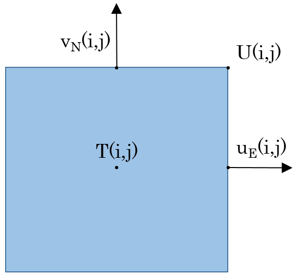
Figure 1 Schematic of a grid cell (i,j) used for the spatial discretization. The indices i and j define the positions of variables, respectively, along the x and y axes. Scalars such as the ice concentration, a, are defined at the T point, while the C-grid velocity components, u_E(i,j) and v_N(i,j), are, respectively, defined at the E and N points. The U point, where both B-grid velocity components are located, is used for some C-grid variables, such as the shear stress, σ₁₂.

For the momentum equation, the most complex part of the C-grid implementation is the spatial discretization of the rheology term (Sect. A3). This involves the calculations of strain rates at the U (Sect. A3.1) and T (Sect. A3.2) points; of ζ, η, and the replacement pressure at the T points (Sect. A3.3); and of η at the U points (Sect. A3.5). No-slip and no-outflow boundary conditions are applied at the land–ocean boundaries using ghost velocities (see Sect. A3.1 for details). Following Bouillon et al. (2013), $D_{\mathrm{s}}^{\mathrm{2}}$ at a T point is obtained from a spatial average of $D_s^{\mathrm{2}}$ from the four neighboring U points. This is done to enhance numerical stability. Following Kimmritz et al. (2016), the code includes two methods for calculating η at the U points; the default method averages η_T from the neighboring ocean cells while the other approach is based on an averaging of the ice strength. Section A3.4 and A3.6 describe the time-stepping of the stresses at the T and U points. The calculation of the x and y components of ∇⋅σ (Sect. A3.7) at the E points (F_1E) and the N points (F_2N) requires σ_1T, σ_2T, and σ_12U. Also, σ_12T is calculated in order to diagnose normalized internal stresses (Lemieux and Dupont, 2020) at the T points.

4 Initial approach for remapping using C-grid velocity components

Considering only the horizontal transport term, we discretize Eq. (8) in terms of partial ice concentration. The transport equation for thickness category n is given by

$$\begin{array}{}\text{(9)}& {\displaystyle \frac{\partial a_n}{\partial t}}+\mathrm{\nabla }\cdot \left(a_n\mathit{u}\right)=\mathrm{0},\end{array}$$

where a_n is the partial ice concentration for category n. Snow volume, ice volume, snow enthalpy, and ice enthalpy also need to be transported using equations of the form

$$\begin{array}{}\text{(10)}& {\displaystyle \frac{\partial \left(a_n{h}_n\right)}{\partial t}}+\mathrm{\nabla }\cdot \left(a_n{h}_n\mathit{u}\right)=\mathrm{0},\text{(11)}& {\displaystyle \frac{\partial \left(a_n{h}_n{q}_n\right)}{\partial t}}+\mathrm{\nabla }\cdot \left(a_n{h}_n{q}_n\mathit{u}\right)=\mathrm{0},\end{array}$$

where h_n is the snow or ice thickness for category n and q_n is the enthalpy.

The incremental remapping scheme solves Eqs. (9)–(11) in a unified way. Given the velocity field u, departure regions are computed for each grid cell. Then the quantities a_n, a_nh_n, and a_nh_nq_n are integrated over each departure region so that volume and internal energy are transferred conservatively between cells.

Our initial implementation of remapping for the C-grid discretization mostly followed that in Lipscomb and Hunke (2004). The differences are related to the interpolation of C-grid velocity components to the U points, as described in Sect. 4.1 below.

4.1 Interpolation of C-grid velocity components and computation of departure regions

Departure regions in the remapping transport scheme are defined by approximating backward trajectories using corner velocities (U points). In our first implementation of remapping for the C-grid, C-grid velocities were interpolated to the corners, and remapping was used in the same way as for the B-grid. The velocity components u_E and v_N are interpolated to the U points as

$$\begin{array}{}\text{(12)}& {\displaystyle }\begin{array}{rl}{u}_U(i,j)& =M_U(i,j)\\ & \times \left[{\displaystyle \frac{u_E(i,j)A_E(i,j)+u_E(i,j+\mathrm{1})A_E(i,j+\mathrm{1})}{A_E(i,j)+A_E(i,j+\mathrm{1})}}\right],\end{array}\text{(13)}& {\displaystyle }\begin{array}{rl}{v}_U(i,j)& =M_U(i,j)\\ & \times \left[{\displaystyle \frac{v_N(i,j)A_N(i,j)+v_N(i+\mathrm{1},j)A_N(i+\mathrm{1},j)}{A_N(i,j)+A_N(i+\mathrm{1},j)}}\right],\end{array}\end{array}$$

where A_E and A_N are grid cell areas evaluated at the E and N points, respectively, and the multiplication by M_U(i,j) ensures that the no-slip and no-outflow boundary conditions (BCs) are respected.

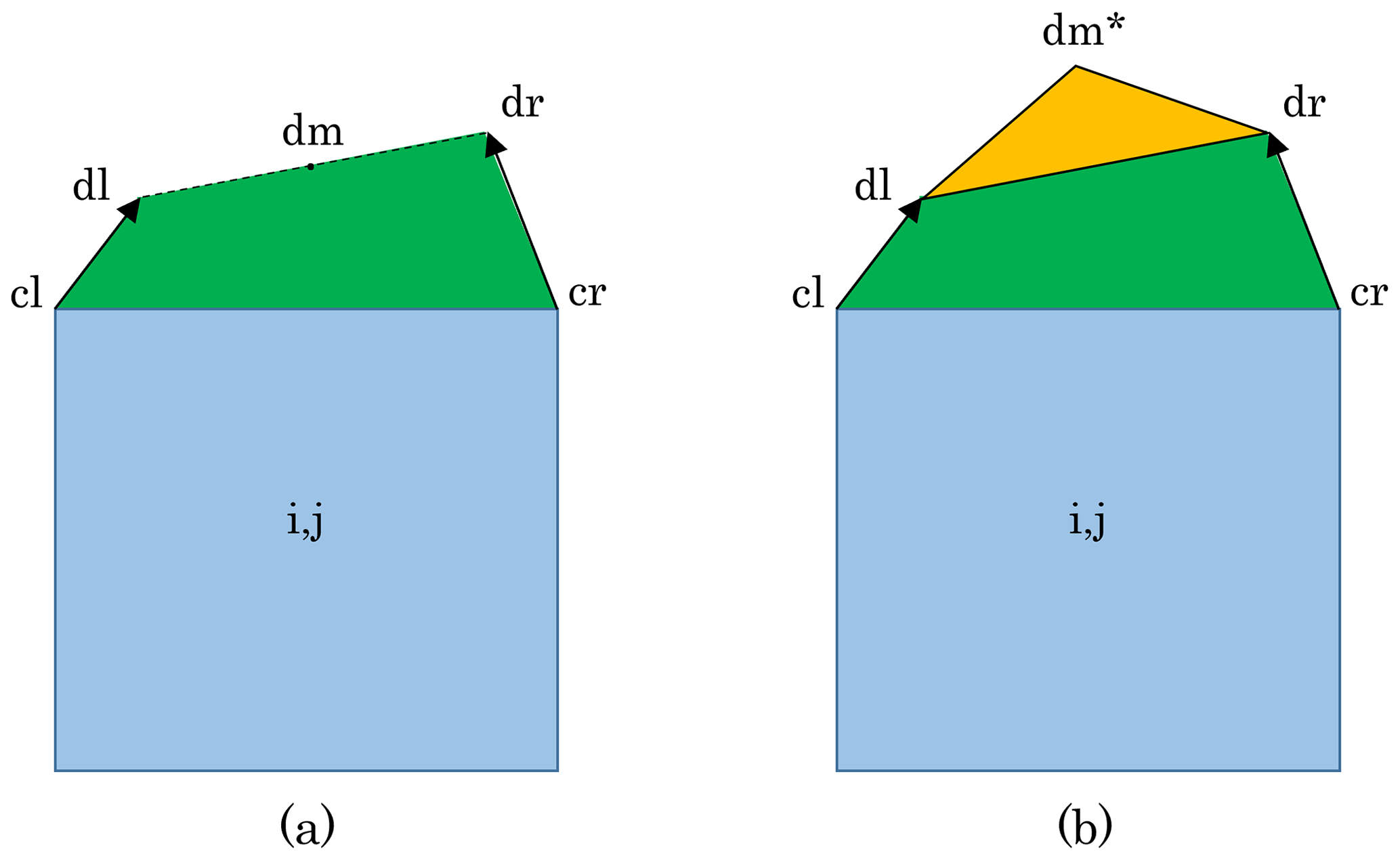
Figure 2 Schematic of departure regions (in green) on the north edge of grid cell (i,j) (in blue) with the standard remapping (a) and the edge flux adjustment method (b). The departure regions are defined by the left corner point (cl), the right corner point (cr), the left departure point (dl), and the right departure point (dr). With the edge flux adjustment method, an additional triangle (in orange) is created by shifting the middle departure point, dm, based on the edge flux associated with v_N(i,j).

To improve the accuracy of the estimated departure regions, the midpoints of the backward trajectories are computed first. Then, velocity components are bilinearly interpolated to these midpoints. Finally, these interpolated velocities are used to calculate the departure points defining the departure regions (Lipscomb and Hunke, 2004).

Panel (a) in Fig. 2 shows an example of a departure region on the north edge of cell (i,j). The departure region is a quadrilateral defined by the left (cl) and right (cr) corner points and the left (dl) and right (dr) departure points.

4.2 Weaknesses of the initial approach for remapping using C-grid velocity components

We identified two notable weaknesses with this initial C-grid discretization and remapping implementation. First, a C-grid discretization offers the possibility of representing transport in one-grid-cell-wide channels, but our initial implementation did not do so. Because of the no-slip and no-outflow BCs, the U velocities are zero on both sides of such a channel, in which case the departure regions have zero area. Second, we found a numerical problem: in some idealized tests, we observed a checkerboard pattern in fields such as sea ice concentration. Panel (a) in Fig. 3 shows an example of this pattern, which indicates the presence of a spurious numerical mode (or modes). This numerical noise is not present when using the upwind scheme (not shown).

Appendix B presents a modal analysis of a simplified set of perturbed equations (momentum and transport). We show that a stationary wave explains the formation of the checkerboard pattern. This stationary wave is a consequence of the spatial averaging used to obtain u_U and v_U (Eqs. 12 and 13) for the remapping scheme.

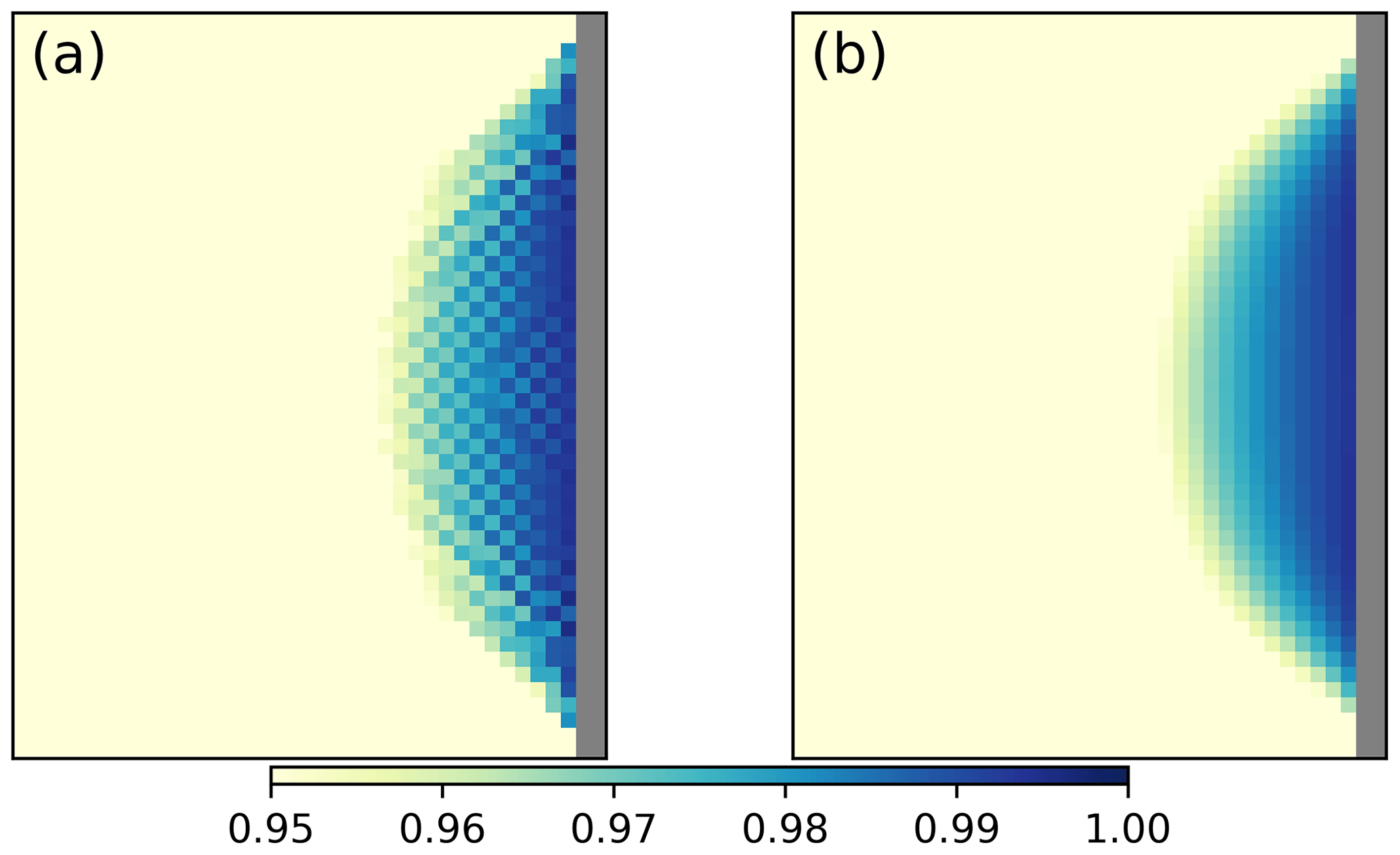
Figure 3 Sea ice concentration field after 15 d for a C-grid simulation with standard remapping (a) or with remapping and the edge flux adjustment method (b). The domain has 80 × 80 grid cells, with $\mathrm{\Delta }x=\mathrm{\Delta }y=\mathrm{16}$ km. The simulation is initialized with a block of ice with a=0.8 and $\stackrel{\mathrm{‾}}{h}=\mathrm{0.8}$ m. The wind blows from the west with a magnitude of 5 m s⁻¹, the Coriolis parameter f set to zero, and the ocean is at rest. The displayed range is 0.95 to 1 in order to better visualize the checkerboard pattern. This experiment is referred to as Exp1. Some information (i.e., physical and numerical parameters) about this experiment is given in Table 1.

5 The edge flux adjustment method

5.1 Description of the method

To eliminate the checkerboard pattern, we introduce a novel approach, which we refer to as the edge flux adjustment (EFA) method. With this method, the remapping scheme still calculates departure regions using the U-point velocities. However, the C-grid velocity components are then used to adjust the edge fluxes (or departure regions.) Following the example in Fig. 2, the departure region is adjusted so that the total flux area A_tot is equal to v_NΔx_NΔt, where Δt is the advective time step and v_N<0 in the example shown in Fig. 2. (Note that A_tot has the same sign as v_n). This is done by shifting the midpoint, dm, of the line segment connecting the departure points, dl and dr. Geometrically speaking, this creates an additional departure triangle (the orange triangle in Fig. 2b).

The code computes the coordinates of the shifted dm in a non-dimensional coordinate system. In this coordinate system, the points cl and cr have the coordinates $(-\mathrm{0.5},\mathrm{0})$ and (0.5,0). The non-dimensional flux area, denoted as ${\stackrel{\mathrm{̃}}{A}}_{\mathrm{tot}}$, is equal to $A_{\mathrm{tot}}/A_N$, where A_N is the grid cell area evaluated at the N point. Given the non-dimensional coordinates (x_dl,y_dl) and (x_dr,y_dr) for the departure points, the non-dimensional coordinates $(x_{\mathrm{dm}}^{*},y_{\mathrm{dm}}^{*})$ for the shifted departure midpoint are obtained as follows:

$$\begin{array}{}\text{(14)}& {\displaystyle }{x}_{\mathrm{dm}}^{*}=x_{\mathrm{dm}}+\mathit{\alpha }(y_{\mathrm{dr}}-y_{\mathrm{dl}}),\text{(15)}& {\displaystyle }{y}_{\mathrm{dm}}^{*}=y_{\mathrm{dm}}-\mathit{\alpha }(x_{\mathrm{dr}}-x_{\mathrm{dl}}),\end{array}$$

where $x_{\mathrm{dm}}=(x_{\mathrm{dl}}+x_{\mathrm{dr}})/\mathrm{2}$ and $y_{\mathrm{dm}}=(y_{\mathrm{dl}}+y_{\mathrm{dr}})/\mathrm{2}$ are the initial departure midpoint coordinates and α is given by

$$\begin{array}{}\text{(16)}& {\displaystyle }\mathit{\alpha }={\displaystyle \frac{\mathrm{2}{\stackrel{\mathrm{̃}}{A}}_{\mathrm{tot}}+(x_{\mathrm{dr}}-x_{\mathrm{cl}})y_{\mathrm{dl}}+(x_{\mathrm{cr}}-x_{\mathrm{dl}})y_{\mathrm{dr}}}{(x_{\mathrm{dr}}-x_{\mathrm{dl}}{)}^{\mathrm{2}}+(y_{\mathrm{dr}}-y_{\mathrm{dl}}{)}^{\mathrm{2}}}}.\end{array}$$

The adjusted area flux can finally be computed using the points $\mathrm{cl}=(x_{\mathrm{cl}},y_{\mathrm{cl}})$, $\mathrm{dl}=(x_{\mathrm{dl}},y_{\mathrm{dl}})$, $\mathrm{cr}=(x_{\mathrm{cr}},y_{\mathrm{cr}})$, $\mathrm{dr}=(x_{\mathrm{dr}},y_{\mathrm{dr}})$, and ${\mathrm{dm}}^{*}=(x_{\mathrm{dm}}^{*},y_{\mathrm{dm}}^{*})$.

The initial departure region shown in Fig. 2a is confined to the central region (i.e., cell (i,j) and/or cell $(i,j+\mathrm{1}))$. When part of the departure region (i.e., a triangle) is located, for example, in a corner cell (e.g., the northwestern cell $(i-\mathrm{1},j+\mathrm{1})$, not shown), the area of this corner triangle is subtracted from A_tot before adjusting the central portion of the departure region (the part lying in cell $(i,j+\mathrm{1})$). In this case, we identify the point (0,y_i) where the segment joining dl and dr intersects the left edge of cell $(i,j+\mathrm{1})$. The departure point dl is reset to (0,y_i) before finding the shifted midpoint, dm^*. Thus, the new triangle with vertices dl, dr, dm^* is always located within the central region.

The calculation of $(x_{\mathrm{dm}}^{*},y_{\mathrm{dm}}^{*})$ as described above is the most common case, with both initial departure points on the same side of the edge (i.e., y_dry_dl≥0). We give another less common example in which y_dr and y_dl have opposite signs. Then, there are two departure triangles: one on the left, with vertices cl, dl, ip, and one on the right, with vertices cr, dr, ip, where ip denotes the point (x_i,0) at which the departure segment intersects the x axis.

In the case shown (Fig. 4), the non-dimensional coordinate x_i of the intersection point is greater than zero. There is a similar case not discussed here, with x_i<0.

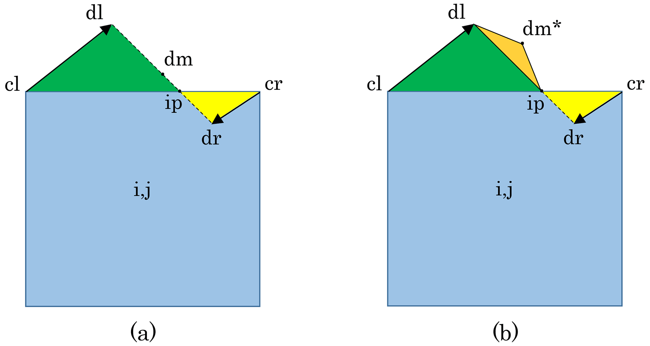
Figure 4 Schematic of departure regions on the north edge of grid cell (i,j) (in blue) with the standard remapping (a) and the edge flux adjustment method (b). The departure region in (a) is defined by the green triangle (with vertices cl, dl, and ip) and the yellow triangle (with vertices cr, dr, and ip). With the EFA method in (b), the departure region has an additional triangle (orange, with vertices ip and dl and shifted middle departure point dm^*). The orange triangle is calculated based on the edge flux associated with v_N(i,j). The yellow triangle is referred to as the “lone triangle”.

The strategy is to fix the right-hand triangle (the “lone triangle”) while modifying the left-hand triangle. Given the required total area flux, A_tot=v_NΔx_NΔt, and the area A_r△ of the right-hand triangle (in yellow), the EFA method first calculates the remaining area flux, $A_l=A_{\mathrm{tot}}-A_{\mathrm{r}\mathrm{△}}$. The middle departure point is reset to $(\frac{x_{\mathrm{dl}}+x_i}{\mathrm{2}},\frac{y_{\mathrm{dl}}}{\mathrm{2}})$, and then dm is shifted so that the non-dimensional area of the green and orange triangles is equal to ${\stackrel{\mathrm{̃}}{A}}_l=A_l/A_N$. The shifted middle departure point has non-dimensional coordinates

$$\begin{array}{}\text{(17)}& {\displaystyle }{x}_{\mathrm{dm}}^{*}=x_{\mathrm{dm}}-\mathit{\alpha }{y}_{\mathrm{dl}},\text{(18)}& {\displaystyle }{y}_{\mathrm{dm}}^{*}=y_{\mathrm{dm}}-\mathit{\alpha }(x_i-x_{\mathrm{dl}}),\end{array}$$

where in this case α is given by

$$\begin{array}{}\text{(19)}& \mathit{\alpha }={\displaystyle \frac{\mathrm{2}{\stackrel{\mathrm{̃}}{A}}_l+(x_i-x_{\mathrm{cl}})y_{\mathrm{dl}}}{(x_i-x_{\mathrm{dl}}{)}^{\mathrm{2}}+y_{\mathrm{dl}}^{\mathrm{2}}}}.\end{array}$$

When a part of the departure region is a corner triangle lying outside cells (i,j) and $(i,j+\mathrm{1})$, it is treated as described above for the most common case.

The EFA method ensures that the divergence (associated with edge fluxes) implied by the remapping is consistent with the divergence calculated by the dynamical solver (i.e., the EVP solver; see Eq. A24). Figure 3b shows that the EFA method prevents the formation of the checkerboard pattern. This pattern originates from an interaction between the solution of the momentum equation and the standard remapping scheme. To support this conclusion, we conducted the following experiment: velocity fields obtained with the C-grid discretization and the use of the EFA method in the remapping scheme were first stored. In a second simulation, both the dynamics (i.e., EVP) and EFA method are turned off and the stored velocity fields are used for transport in the remapping scheme. In this case, no checkerboard pattern develops, and the concentration field is very similar to the one shown in Fig. 3b.

The EFA code was added to the standard CICE remapping algorithm described in Lipscomb and Hunke (2004). Although the remapping algorithm for the B-grid is very robust, we found that some approximations in the computation of departure regions can be problematic with the new EFA method for the C-grid discretization. Long-term C-grid simulations with the EFA method exhibited rare failures on non-uniform grids. The remapping code in CICE includes many consistency checks to ensure that the solution is physically sound – for example, that transport does not lead to negative area or mass. The code failed on rare occasions with negative area and mass values close to land or the ice edge. These negative values were a result of approximations in the area of the departure region. Appendix C describes the changes in the remapping algorithm that were required to fix this robustness issue. Note that many of these modifications slightly alter the departure areas for both the B-grid and the C-grid (with the EFA method) discretizations. With these changes to the remapping, the algorithm is now robust for both B-grid and C-grid simulations on non-uniform grids.

5.2 Transport through one-grid-cell-wide channels

Interestingly, the EFA method also remedies the other weakness of our initial implementation: the absence of transport in one-grid-cell-wide channels. Although the initial departure regions have zero area (because the U-point velocities are zero along the channel edges), the departure regions are adjusted based on C-grid velocity components (e.g., the v_N component would be non-zero for a north–south channel). In this case, the departure region is simply defined by (x_cl,y_cl), (x_cr,y_cr), and $(x_{\mathrm{dm}}^{*},y_{\mathrm{dm}}^{*})$, with $x_{\mathrm{dm}}^{*}=\mathrm{0}$.

A minor code modification was required nevertheless. Before this modification, the edge fluxes were calculated only when at least one of the two departure points was displaced from its corner. Given the non-displaced departure points for the north edge (i.e., $u_U(i-\mathrm{1},j)=v_U(i-\mathrm{1},j)=\mathrm{0}$ and $u_U(i,j)=v_U(i,j)=\mathrm{0}$), edge fluxes are now computed whenever $\left|v_N\mathrm{\Delta }{x}_N\mathrm{\Delta }t\right|>\mathrm{0}$. Similarly for the east edge (i.e., $u_U(i,j)=v_U(i,j)=\mathrm{0}$ and $u_U(i,j-\mathrm{1})=v_U(i,j-\mathrm{1})=\mathrm{0}$), edge fluxes are now computed whenever $\left|u_E\mathrm{\Delta }{y}_E\mathrm{\Delta }t\right|>\mathrm{0}$. Given that the remapping with the EFA method uses velocity components at the U point and at the E and N points and that it allows for transport in one-grid-cell-wide channels, it should be viewed as a hybrid B-and-C-grid approach.

To test the new capability for transport, we implemented an idealized configuration with a long one-grid-cell-wide channel. The initial ice conditions are a=0.5 and $\stackrel{\mathrm{‾}}{h}=\mathrm{1}$ m over a length of five grid cells (80 km), with a=0 and $\stackrel{\mathrm{‾}}{h}=\mathrm{0}$ m elsewhere. The wind blows from the west, and the fields are analyzed after 30 d of simulation. As expected, there is no transport with the B-grid discretization (not shown). Using the C-grid discretization, both the upwind method and the remapping with the EFA method lead to transport in the channel (Fig. 5). As shown by Lipscomb and Hunke (2004) for more complex configurations, remapping is much less diffusive than upwind.

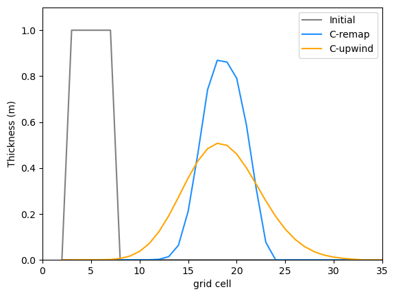
Figure 5 Simulated thickness after 30 d along a one-grid-cell-wide channel for the C-grid with remapping (blue) and upwind (orange). These simulations were initialized with a=0.5 and $\stackrel{\mathrm{‾}}{h}=\mathrm{1}$ m over a region that is five grid cells long (gray). The wind blows from the west at 5 m s⁻¹, $\mathrm{\Delta }x=\mathrm{\Delta }y=\mathrm{16}$ km, and the ocean is at rest. This experiment is referred to as Exp2 in Table 1.

6 Validation of the C-grid implementation

We validated the new C-grid implementation with the EFA method using several approaches, including (1) symmetry tests, (2) thorough comparison of C-grid simulations with the default B-grid simulations, (3) comparison of C-grid simulations with analytical solutions, and (4) diagnostics of simulated stress states. This section gives an overview of the different tests. For all the simulations presented here, we used version 6.5.0 of CICE, which includes our C-grid modifications. Unless otherwise specified, we used default values for most physical and numerical parameters. In the experiments described below, we mostly modified the strength parameterization, P^*, Δ_min, the number of EVP subcycles (n_evp), and E₀, in order to broaden the variety of tests (e.g., ice strength parameterization) and in some cases to improve the numerical convergence of the EVP method (n_evp and E₀). See Table 1 for experiment details.

We conducted many idealized tests to verify the symmetry of simulated fields. Figure 6 shows an example. The thickness fields after 14 d are perfectly (bit-for-bit) symmetrical for the four oblique (i.e., northeast, southeast, southwest, and northwest) wind directions. Similar tests with the wind blowing from the west, east, north, and south also give symmetrical results, but with small differences (the maximum difference is 4 × 10⁻⁴ m). Changing the capping method to the smoother formulation (i.e., capping_method = 'sum') leads to bit-for-bit symmetrical results.

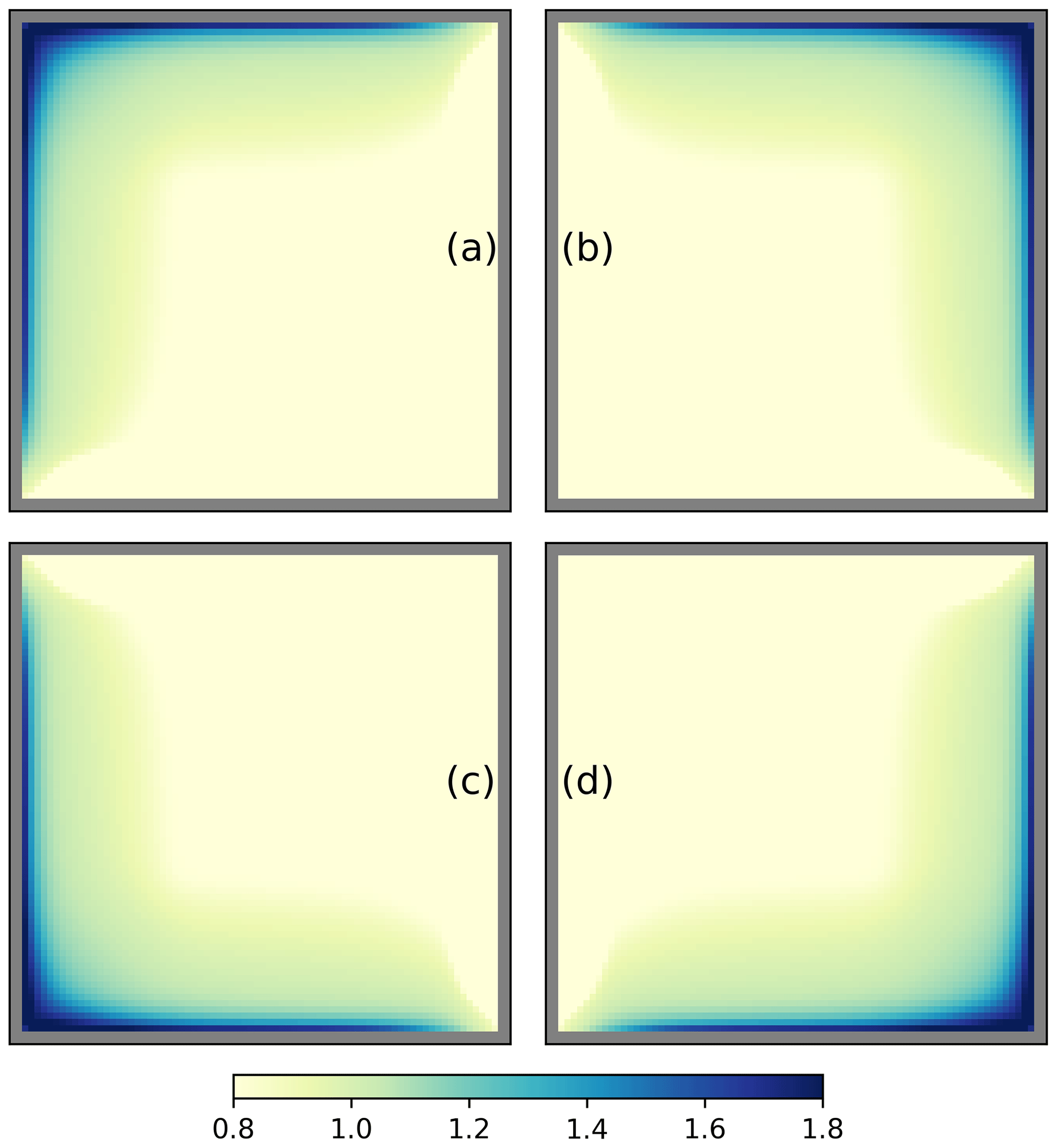
Figure 6 Simulated sea ice thickness after 14 d for winds blowing toward the northwest (a), northeast (b), southwest (c), and southeast (d). The domain has 80 × 80 grid cells, with $\mathrm{\Delta }x=\mathrm{\Delta }y=\mathrm{16}$ km. The simulation is initialized with uniform ice conditions, with a=0.8 and $\stackrel{\mathrm{‾}}{h}=\mathrm{0.8}$ m. The wind components have values of ±5 m s⁻¹. The ocean is at rest and f=0. This experiment is referred to as Exp3 in Table 1.

We also evaluated more realistic simulations with B-grid runs as references. We compared C-grid runs on 1 and 3° global grids to B-grid runs initialized and forced by the same fields. The Japanese 55-year Reanalysis (JRA-55; Kobayashi et al., 2015) is used for the atmospheric forcing fields, while the ocean forcing was derived from a Community Earth System Model (CESM) simulation (Kay et al., 2015). Panels (a) and (b), respectively, in Fig. 7 show the total simulated sea ice volume for the Northern and Southern hemispheres for a 1° B-grid simulation with remapping transport (reference, orange), a 1° B-grid simulation with upwind transport (blue), and a 1° C-grid simulation with remapping transport (dashed violet). Only the C-grid simulation uses the EFA method. Compared to the reference B-grid simulation, changing the grid discretization has a smaller impact on the total volume than changing the advection scheme. This is particularly evident in the Southern Hemisphere.

Table 1 Table of some physical and numerical parameters used for the experiments.

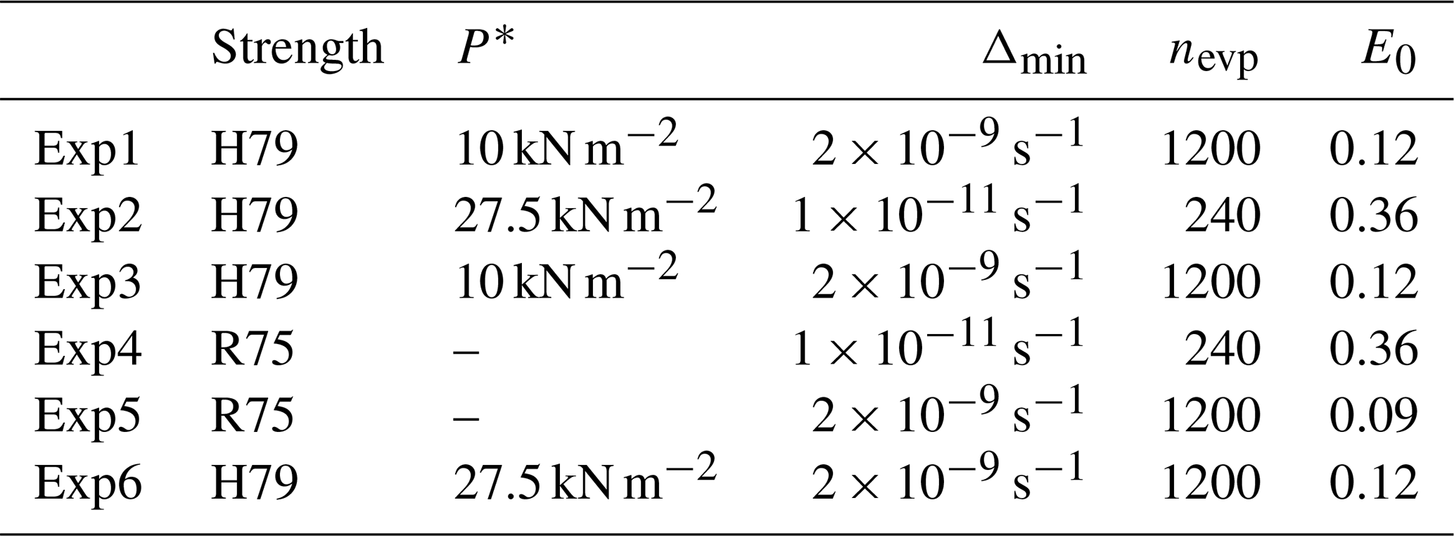
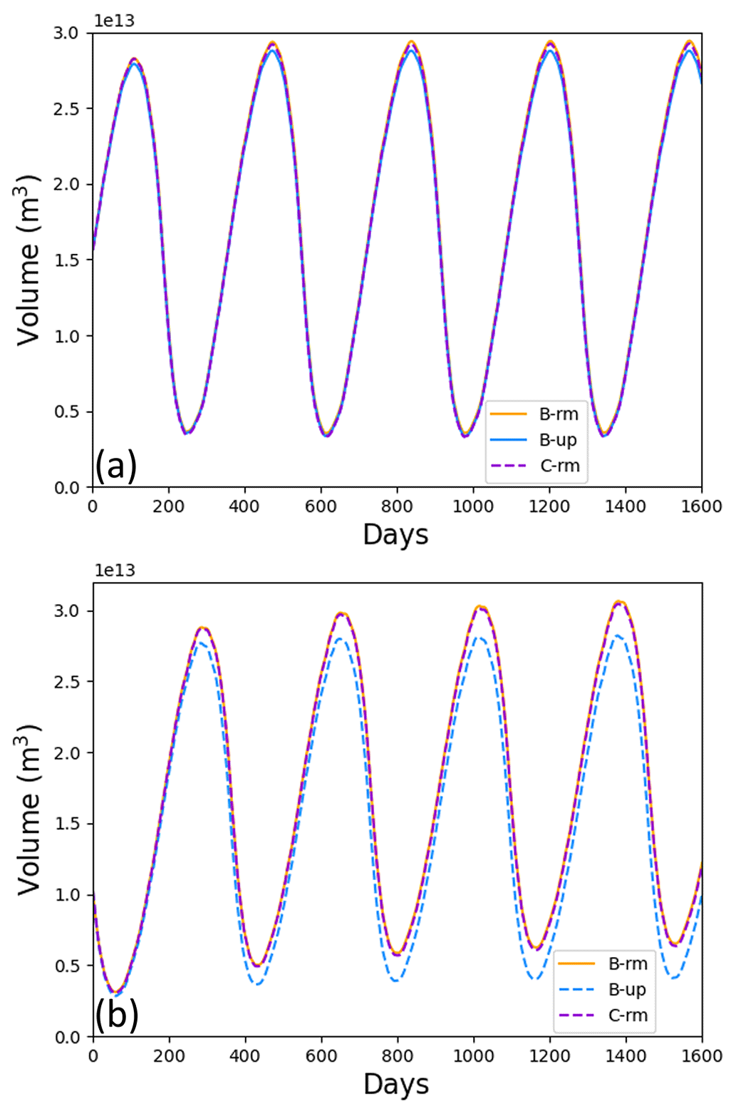
Figure 7 Simulated sea ice volume in the Northern Hemisphere (a) and the Southern Hemisphere (b) as a function of time for the B-grid with remapping transport (orange), the B-grid with upwind transport (blue), and the C-grid with remapping transport (dashed violet). These are 5-year simulations on a 1° global grid initialized from a long simulation. This experiment is referred to as Exp4 in Table 1.

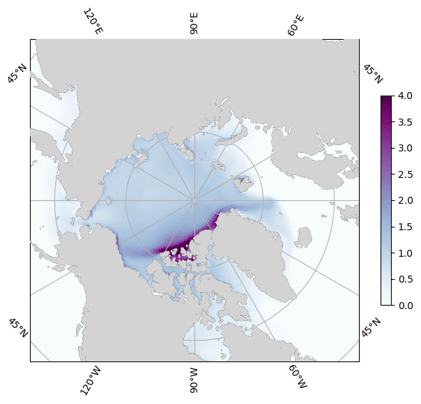
Figure 8 Monthly mean sea ice thickness (m) after 5 years (December 2009) for a 1° C-grid simulation with the remapping transport scheme. This experiment is referred to as Exp4 in Table 1.

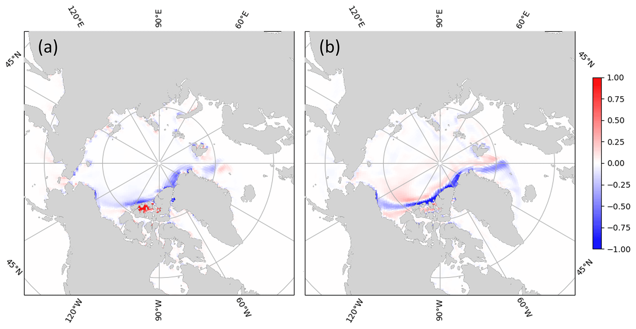
Figure 9 Difference in the monthly mean sea ice thickness (m) after 5 years (December 2009) between a 1° C-grid simulation with remapping and a 1° B-grid simulation with remapping (reference) (a). Difference in the monthly mean sea ice thickness after 5 years (December 2009) between a 1° B-grid simulation with upwind and a 1° B-grid simulation with remapping (reference) (b). This experiment is referred to as Exp4 in Table 1.

This conclusion is further supported by spatial maps of sea ice thickness. The monthly mean ice thickness in December 2009 for a 1° C-grid simulation with remapping is qualitatively correct, with the thickest ice found north of Greenland and in the Canadian Arctic Archipelago (Fig. 8). When compared to the reference simulation (B-grid with remapping), the ice is thinner in the regions of thick ice (Fig. 9a), although these differences are generally less pronounced than those for a B-grid with upwind compared to the reference (Fig. 9b). The same is true for the Southern Hemisphere (not shown).

The checkerboard pattern was not visible in our initial 1 and 3° C-grid simulations without EFA. Instead, the error manifested as much thicker ice in convergent regions. We speculate this was due to a feedback between excessive ridging associated with the checkerboard pattern in velocities (and hence divergence and convergence) and ice growth in open water formed through the ridging process.

The most complex part of the discretization of the momentum equation is the rheology term. A crucial test is to verify whether the simulated internal stresses are inside (viscous) or on (plastic) the elliptical yield curve. To improve the numerical convergence of the EVP solver, the number of subcycling iterations, n_evp, was increased from 240 (default) to 1200 and the elastic damping parameter, E₀, was reduced from 0.36 (default) to 0.09 (Exp5 in Table 1). Following the approach of Lemieux and Dupont (2020), we plotted the states of stress in stress-invariant coordinates of a snapshot after 5 d of a 1° C-grid simulation. Figure 10 confirms that the solution is viscous–plastic.

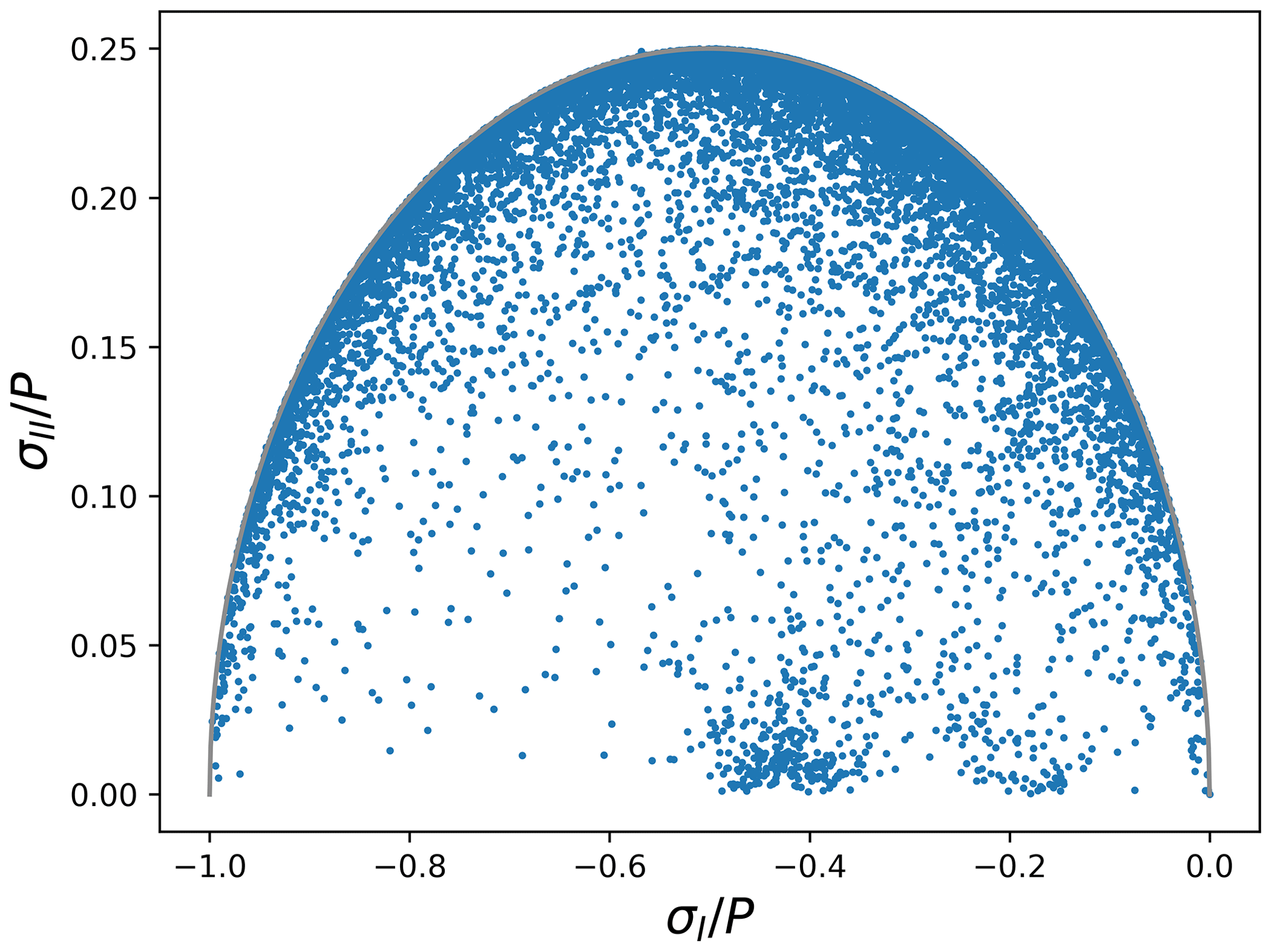
Figure 10 Stress invariants, σ_I and σ_II, normalized by the ice strength, P. These are obtained from a snapshot after 5 d of a 1° C-grid simulation. This experiment is referred to as Exp5 in Table 1.

Analytical solutions are useful tools for verifying a numerical implementation. We derived novel analytical solutions for a one-grid-cell-wide channel with cyclic boundary conditions; see Appendix D for the derivation. As sea ice conditions are assumed constant in space and time, these solutions cannot be used to verify the simulated transport. Nevertheless, they provide steady-state analytical velocity values. Following the assumptions of this analytical solution with a=0.8 and $\stackrel{\mathrm{‾}}{h}=\mathrm{0.8}$ m for an east–west channel, the ice should be in the plastic (viscous) regime for wind speeds higher (lower) than $u_{\mathrm{a}*}=\mathrm{3.176}$ m s⁻¹. For u_a=4 m s⁻¹ (i.e., $u_{\mathrm{a}}>u_{\mathrm{a}*}$), the steady-state analytical solution, u_E, calculated independently using a Python code is 0.04095 m s⁻¹. The steady-state solution, u_E, obtained with the new C-grid implementation matches the analytical solution up to the 12th digit. Similarly, for u_a=1.5 m s⁻¹ (i.e., $u_{\mathrm{a}}<u_{\mathrm{a}*}$), the steady-state analytical solution u_E is much smaller and is equal to 7.135 × 10⁻⁶ m s⁻¹. The new C-grid steady-state solution, u_E, matches the analytical solution up to the ninth digit (a difference of less than 10⁻¹⁶ m s⁻¹). The same results are found when using a north–south channel. This experiment is referred to as Exp6 in Table 1.

7 Conclusions

We have designed and implemented a C-grid version of the CICE sea ice model. The C-grid spatial discretization is based on a finite-difference approach and follows the work of Bouillon et al. (2009, 2013) and Kimmritz et al. (2016). This article describes the finite-difference spatial discretization of the momentum equation, the implementation of no-slip and no-outflow boundary conditions, and the use of the remapping transport scheme with C-grid velocities.

The most notable contribution of this work is a novel method for the remapping referred to as the edge flux adjustment (EFA) method. Preliminary results from idealized experiments showed that the new C-grid discretization for the momentum equation and the use of the standard remapping transport scheme could produce checkerboard patterns in fields such as ice concentration. This numerical noise is not present when using the upwind transport scheme. A modal analysis of a simplified set of perturbed equations (i.e., momentum and transport with spatial discretization) shows that a stationary wave is responsible for the checkerboard pattern. This stationary wave results from the interpolation of C-grid velocity components to the U points for use with remapping, which is fundamentally a B-grid scheme (Dukowicz and Baumgardner, 2000; Lipscomb and Hunke, 2004). This interpolation can be viewed as a spatial averaging. Many authors (e.g., Batteen and Han, 1981) have demonstrated that spatial averaging can lead to checkerboard patterns when solving the shallow-water equations, which are similar to our simplified set of equations. The checkerboard pattern is eliminated by the EFA method.

The EFA method uses C-grid velocity components at their natural locations to modify the departure regions calculated by the remapping so that the implied divergence in the remapping is consistent with the divergence calculated by the dynamical solver. We also introduced some modifications to the calculation of the area of departure regions to increase the robustness of remapping with the EFA method on non-uniform grids.

A C-grid discretization offers the possibility of representing transport in one-grid-cell-wide channels. Because of the no-slip and no-outflow boundary conditions, the U-point velocities at the channel edges are zero, and there is therefore no transport when using the standard remapping. The EFA method, however, allows for transport in these channels by creating departure regions with non-zero area based on the C-grid velocities. As such, the remapping with the EFA method should be seen as a hybrid B-and-C-grid transport scheme. Moreover, remapping with the EFA method is much less diffusive than the upwind method for idealized channel tests.

For VP sea ice models, there are few existing analytical solutions due to the complexity of the rheology. We derived novel analytical solutions for one-grid-cell-wide channels and showed that with several simplifications (uniform ice conditions, constant wind, cyclic boundary conditions, and transport turned off), the sea ice velocity can be obtained analytically for both plastic and viscous regimes. The steady-state values simulated by CICE match the analytical ones.

We also conducted multiyear 1° global simulations to compare the C-grid solution (using the EFA method) to the reference B-grid solution (with standard remapping). We ran an additional B-grid simulation with upwind transport. Compared to the reference B-grid run, the C-grid discretization has a smaller impact on the total volume (and spatial differences) than changing the advection scheme from remapping to upwind, especially in the Southern Hemisphere.

Ongoing work within CICE Consortium modeling centers includes coupling this new CICE C-grid implementation to ocean models, such as the Modular Ocean Model (MOM6) and the Nucleus for European Modelling of the Ocean (NEMO), and to atmospheric models, such as the Global Environmental Multiscale Model (GEM).

Appendix A: Spatial and temporal discretization of the momentum equation

The spatial discretization is presented below in the same order as in the code.

A1 Air stress at the E and N points

For both B-grid and C-grid implementations, the air stress is calculated at the T point and then interpolated to the required locations. For the C-grid, τ_ax at the E point and τ_ay at the N point are weighted averages of the values at the neighboring T points and are given by

$$\begin{array}{}\text{(A1)}& {\displaystyle }\begin{array}{rl}{\mathit{\tau }}_{\mathrm{a}xE}(i,j)& ={\displaystyle \frac{\mathrm{1}}{\mathrm{2}{A}_E(i,j)}}\left[{\mathit{\tau }}_{\mathrm{a}xT}(i,j)A_T(i,j)\right.\\ & \left.+{\mathit{\tau }}_{\mathrm{a}xT}(i+\mathrm{1},j)A_T(i+\mathrm{1},j)\right],\end{array}\text{(A2)}& {\displaystyle }\begin{array}{rl}{\mathit{\tau }}_{\mathrm{a}yN}(i,j)& ={\displaystyle \frac{\mathrm{1}}{\mathrm{2}{A}_N(i,j)}}\left[{\mathit{\tau }}_{\mathrm{a}yT}(i,j)A_T(i,j)\right.\\ & \left.+{\mathit{\tau }}_{\mathrm{a}yT}(i,j+\mathrm{1})A_T(i,j+\mathrm{1})\right],\end{array}\end{array}$$

where A_E, A_N, and A_T are cell areas evaluated at the E, N, and T points.

A2 Seabed stress at the E and N points

The seabed stress components are ${\mathit{\tau }}_{bxE}=-C_{bE}{u}_E$ and ${\mathit{\tau }}_{byN}=-C_{bN}{v}_N$, where the C_b coefficients are calculated as in Lemieux et al. (2016) or following the probabilistic approach of Dupont et al. (2022). For both approaches, C_bE and C_bN are written as

$$\begin{array}{}\text{(A3)}& {\displaystyle }{C}_{bE}(i,j)={\displaystyle \frac{T_{bE}(i,j)}{\left(\sqrt{u_E^{\mathrm{2}}(i,j)+v_E^{\mathrm{2}}(i,j)}+u_{\mathrm{0}}\right)}},\text{(A4)}& {\displaystyle }{C}_{bN}(i,j)={\displaystyle \frac{T_{bN}(i,j)}{\left(\sqrt{u_N^{\mathrm{2}}(i,j)+v_N^{\mathrm{2}}(i,j)}+u_{\mathrm{0}}\right)}},\end{array}$$

where T_bE and T_bN are factors that characterize the maximum possible seabed stress and u₀ is a small velocity parameter that ensures a smooth transition between the static and dynamic regimes of the seabed stress. Velocity v_E is obtained by interpolating v_N to the E point, and u_N is found similarly by interpolating u_E to the N point. These interpolations are currently different than in the C-grid implementation of Lemieux et al. (2015) but will be made consistent in a subsequent version of CICE.

As opposed to the denominators in Eqs. (A3) and (A4), factors T_bE and T_bN do not vary during the EVP subcycling. They are therefore calculated before the subcycling. Following the approach of Lemieux et al. (2016), T_bE and T_bN are

$$\begin{array}{}\text{(A5)}& {\displaystyle }{T}_{bE}(i,j)=k_{\mathrm{2}}max[\mathrm{0},({\stackrel{\mathrm{‾}}{h}}_E-h_{cE}\left)\right]e^{-{\mathit{\alpha }}_b(\mathrm{1}-a_E)},\text{(A6)}& {\displaystyle }{T}_{bN}(i,j)=k_{\mathrm{2}}max[\mathrm{0},({\stackrel{\mathrm{‾}}{h}}_N-h_{cN}\left)\right]e^{-{\mathit{\alpha }}_b(\mathrm{1}-a_N)},\end{array}$$

where ${\stackrel{\mathrm{‾}}{h}}_E=max\left[{\stackrel{\mathrm{‾}}{h}}_T\right(i,j),{\stackrel{\mathrm{‾}}{h}}_T(i+\mathrm{1},j\left)\right]$; $a_E=max\left[a_T\right(i,j),a_T(i+\mathrm{1},j\left)\right]$; $h_{cE}=a_E{h}_{\mathrm{w}E}/k_{\mathrm{1}}$, $h_{\mathrm{w}E}=min\left[h_{\mathrm{w}T}\right(i,j),h_{\mathrm{w}T}(i+\mathrm{1},j\left)\right]$; ${\stackrel{\mathrm{‾}}{h}}_N=max\left[{\stackrel{\mathrm{‾}}{h}}_T\right(i,j),{\stackrel{\mathrm{‾}}{h}}_T(i,j+\mathrm{1}\left)\right]$; $a_N=max\left[a_T\right(i,j),a_T(i,j+\mathrm{1}\left)\right]$; and $h_{cN}=a_N{h}_{\mathrm{w}N}/k_{\mathrm{1}}$, $h_{\mathrm{w}N}=min\left[h_{\mathrm{w}T}\right(i,j),h_{\mathrm{w}T}(i,j+\mathrm{1}\left)\right]$. ${\stackrel{\mathrm{‾}}{h}}_E$ (${\stackrel{\mathrm{‾}}{h}}_N$), h_cE (h_cN), and h_wE (h_wN) are the mean ice thickness (or ice volume), the critical thickness, and the water depth at the E (N) point calculated using values at the T point. k₁, k₂, and α_b are three parameters of the seabed stress parameterization (Lemieux et al., 2016). The T_b factors are set to zero when the water depth is greater than 30 m.

When the seabed stress is computed based on the probabilistic approach, the calculation of the T_b factors is more complicated than with the method of Lemieux et al. (2016). Details can be found in Dupont et al. (2022). With the probabilistic approach, the T_b factor is first calculated at the T points, and T_bE and T_bN are then given by

$$\begin{array}{}\text{(A7)}& {\displaystyle }{T}_{bE}(i,j)=max\left[T_{bT}\right(i,j),T_{bT}(i+\mathrm{1},j\left)\right],\text{(A8)}& {\displaystyle }{T}_{bN}(i,j)=max\left[T_{bT}\right(i,j),T_{bT}(i,j+\mathrm{1}\left)\right].\end{array}$$

A3 Discretization of rheology

As opposed to the variational method used for the B-grid (Hunke and Dukowicz, 1997, 2002), our C-grid spatial discretization is based on finite differences. With this approach, the discretization of ∇⋅σ requires the calculation of σ₁ and σ₂ at the T points and of σ₁₂ at the U points. The stresses are calculated in three steps: the computation of strain rates, the computation of viscosities and replacement pressure, and finally the time-stepping of the stresses from subcycle k to k+1. The subsections below explain how this is done for the T and U points. The sequence of computations follows that in the code.

The spatial discretization requires the computation of strain rates and components of the rheology term in curvilinear coordinates. The strain rates are given by

$$\begin{array}{}\text{(A9)}& {\displaystyle }{D}_{\mathrm{d}}={\dot{\mathit{ϵ}}}_{\mathrm{11}}+{\dot{\mathit{ϵ}}}_{\mathrm{22}}={\displaystyle \frac{\mathrm{1}}{h_{\mathrm{1}}{h}_{\mathrm{2}}}}\left[{\displaystyle \frac{\partial }{\partial {\mathit{\xi }}_{\mathrm{1}}}}\left(h_{\mathrm{2}}u\right)+{\displaystyle \frac{\partial }{\partial {\mathit{\xi }}_{\mathrm{2}}}}\left(h_{\mathrm{1}}v\right)\right],\text{(A10)}& {\displaystyle }{D}_{\mathrm{t}}={\dot{\mathit{ϵ}}}_{\mathrm{11}}-{\dot{\mathit{ϵ}}}_{\mathrm{22}}={\displaystyle \frac{h_{\mathrm{2}}}{h_{\mathrm{1}}}}{\displaystyle \frac{\partial }{\partial {\mathit{\xi }}_{\mathrm{1}}}}\left({\displaystyle \frac{u}{h_{\mathrm{2}}}}\right)-{\displaystyle \frac{h_{\mathrm{1}}}{h_{\mathrm{2}}}}{\displaystyle \frac{\partial }{\partial {\mathit{\xi }}_{\mathrm{2}}}}\left({\displaystyle \frac{v}{h_{\mathrm{1}}}}\right),\text{(A11)}& {\displaystyle }{D}_{\mathrm{s}}=\mathrm{2}{\dot{\mathit{ϵ}}}_{\mathrm{12}}={\displaystyle \frac{h_{\mathrm{1}}}{h_{\mathrm{2}}}}{\displaystyle \frac{\partial }{\partial {\mathit{\xi }}_{\mathrm{2}}}}\left({\displaystyle \frac{u}{h_{\mathrm{1}}}}\right)+{\displaystyle \frac{h_{\mathrm{2}}}{h_{\mathrm{1}}}}{\displaystyle \frac{\partial }{\partial {\mathit{\xi }}_{\mathrm{1}}}}\left({\displaystyle \frac{v}{h_{\mathrm{2}}}}\right),\end{array}$$

where D_d is the divergence, D_t is the tension, D_s is the shear strain rate, ξ₁ and ξ₂ are the non-dimensional coordinates, and h₁ and h₂ are scale factors, referred to as Δx and Δy.

In curvilinear coordinates, the x and y components of the divergence of the stress tensor are, respectively, as follows:

$$\begin{array}{}\text{(A12)}& {\displaystyle }{F}_{\mathrm{1}}={\displaystyle \frac{\mathrm{1}}{\mathrm{2}}}\left[{\displaystyle \frac{\mathrm{1}}{h_{\mathrm{1}}}}{\displaystyle \frac{\partial {\mathit{\sigma }}_{\mathrm{1}}}{\partial {\mathit{\xi }}_{\mathrm{1}}}}+{\displaystyle \frac{\mathrm{1}}{h_{\mathrm{1}}{h}_{\mathrm{2}}^{\mathrm{2}}}}{\displaystyle \frac{\partial \left(h_{\mathrm{2}}^{\mathrm{2}}{\mathit{\sigma }}_{\mathrm{2}}\right)}{\partial {\mathit{\xi }}_{\mathrm{1}}}}+{\displaystyle \frac{\mathrm{2}}{h_{\mathrm{1}}^{\mathrm{2}}{h}_{\mathrm{2}}}}{\displaystyle \frac{\partial \left(h_{\mathrm{1}}^{\mathrm{2}}{\mathit{\sigma }}_{\mathrm{12}}\right)}{\partial {\mathit{\xi }}_{\mathrm{2}}}}\right],\text{(A13)}& {\displaystyle }{F}_{\mathrm{2}}={\displaystyle \frac{\mathrm{1}}{\mathrm{2}}}\left[{\displaystyle \frac{\mathrm{1}}{h_{\mathrm{2}}}}{\displaystyle \frac{\partial {\mathit{\sigma }}_{\mathrm{1}}}{\partial {\mathit{\xi }}_{\mathrm{2}}}}-{\displaystyle \frac{\mathrm{1}}{h_{\mathrm{1}}^{\mathrm{2}}{h}_{\mathrm{2}}}}{\displaystyle \frac{\partial \left(h_{\mathrm{1}}^{\mathrm{2}}{\mathit{\sigma }}_{\mathrm{2}}\right)}{\partial {\mathit{\xi }}_{\mathrm{2}}}}+{\displaystyle \frac{\mathrm{2}}{h_{\mathrm{1}}{h}_{\mathrm{2}}^{\mathrm{2}}}}{\displaystyle \frac{\partial \left(h_{\mathrm{2}}^{\mathrm{2}}{\mathit{\sigma }}_{\mathrm{12}}\right)}{\partial {\mathit{\xi }}_{\mathrm{1}}}}\right],\end{array}$$

which are Eqs. (20) and (21) in Hunke and Dukowicz (2002).

A3.1 Strain rates at the U points

To solve the momentum equation, shear stress, σ₁₂, is needed at the U points, including at land–ocean boundaries. This implies that strain rates and shear viscosities must be computed at these locations. In the code, strain rates at the U points are first calculated. The reason for doing this is to follow what is suggested in Bouillon et al. (2013); to enhance numerical stability, $D_{\mathrm{s}T}^{\mathrm{2}}$ in Δ_T is a weighted average of the $D_{\mathrm{s}U}^{\mathrm{2}}$ around it.

As described in Sect. A3.5, there are two methods for calculating η at the U points. Following Kimmritz et al. (2016), we refer to these methods as C1 and C2. The C1 method requires only D_sU, while the C2 method requires D_dU, D_tU, and D_sU. C1 is the default method, but for completeness, we explain here how D_dU, D_tU, and D_sU are computed.

To ease the implementation of the boundary conditions (BCs) in the code, strain rates at the U points are calculated differently than at the T points. To do so, the derivatives in Eqs. (A9), (A10), and (A11) are expanded. First, for the divergence, Eq. (A9), we expand the derivatives and write

$$\begin{array}{}\text{(A14)}& D_{\mathrm{d}}={\displaystyle \frac{\mathrm{1}}{h_{\mathrm{1}}{h}_{\mathrm{2}}}}\left[h_{\mathrm{2}}{\displaystyle \frac{\partial u}{\partial {\mathit{\xi }}_{\mathrm{1}}}}+u{\displaystyle \frac{\partial h_{\mathrm{2}}}{\partial {\mathit{\xi }}_{\mathrm{1}}}}+h_{\mathrm{1}}{\displaystyle \frac{\partial v}{\partial {\mathit{\xi }}_{\mathrm{2}}}}+v{\displaystyle \frac{\partial h_{\mathrm{1}}}{\partial {\mathit{\xi }}_{\mathrm{2}}}}\right].\end{array}$$

The discretized form of divergence at the U point (i,j) is therefore

$$\begin{array}{}\text{(A15)}& \begin{array}{rl}{D}_{\mathrm{d}U}(i,j)& ={\displaystyle \frac{\mathrm{1}}{h_{\mathrm{1}U}(i,j)h_{\mathrm{2}U}(i,j)}}\\ & \times \left[h_{\mathrm{2}U}\right(i,j\left)\right(u_N^{*}(i+\mathrm{1},j)-u_N^{*}(i,j))\\ & +u_U(i,j)\left(h_{\mathrm{2}N}\right(i+\mathrm{1},j)-h_{\mathrm{2}N}(i,j\left)\right)\\ & +h_{\mathrm{1}U}(i,j)\left(v_E^{*}\right(i,j+\mathrm{1})-v_E^{*}(i,j\left)\right)\\ & +v_U(i,j)\left(h_{\mathrm{1}E}\right(i,j+\mathrm{1})-h_{\mathrm{1}E}(i,j\left)\right)],\end{array}\end{array}$$

where $u_N^{*}(i+\mathrm{1},j)$, $u_N^{*}(i,j)$, $v_E^{*}(i,j+\mathrm{1})$, and $v_E^{*}(i,j)$ are modified versions of $u_N(i+\mathrm{1},j)$, u_N(i,j), $v_E(i,j+\mathrm{1})$, and v_E(i,j) to take the BCs into account. This is explained below. The velocity components interpolated to the U points follow Eqs. (12) and (13), while (the unmodified) v_E and u_N are calculated as

$$\begin{array}{}\text{(A16)}& {\displaystyle }{v}_E(i,j)={\displaystyle \frac{\mathrm{1}}{A_{N\mathrm{tot}}}}\sum _{k=\mathrm{0}}^{\mathrm{1}}\sum _{l=-\mathrm{1}}^{\mathrm{0}}{v}_N(i+k,j+l)A_N(i+k,j+l),\text{(A17)}& {\displaystyle }{u}_N(i,j)={\displaystyle \frac{\mathrm{1}}{A_{E\mathrm{tot}}}}\sum _{k=-\mathrm{1}}^{\mathrm{0}}\sum _{l=\mathrm{0}}^{\mathrm{1}}{u}_E(i+k,j+l)A_E(i+k,j+l),\end{array}$$

where $A_{N\mathrm{tot}}={\sum }_{k=\mathrm{0}}^{\mathrm{1}}{\sum }_{l=-\mathrm{1}}^{\mathrm{0}}{A}_N(i+k,j+l)$ and $A_{E\mathrm{tot}}={\sum }_{k=-\mathrm{1}}^{\mathrm{0}}{\sum }_{l=\mathrm{0}}^{\mathrm{1}}{A}_E(i+k,j+l)$. For example, to clarify the notation, $A_{N\mathrm{tot}}={\sum }_{k=\mathrm{0}}^{\mathrm{1}}{\sum }_{l=-\mathrm{1}}^{\mathrm{0}}{A}_N(i+k,j+l)=A_N(i,j-\mathrm{1})+A_N(i,j)+A_N(i+\mathrm{1},j-\mathrm{1})+A_N(i+\mathrm{1},j)$.

Similarly, to calculate D_t at the U points, we expand the derivatives in Eq. (A10) and write the tension as

$$\begin{array}{}\text{(A18)}& D_{\mathrm{t}}={\displaystyle \frac{\mathrm{1}}{h_{\mathrm{1}}{h}_{\mathrm{2}}}}\left[h_{\mathrm{2}}{\displaystyle \frac{\partial u}{\partial {\mathit{\xi }}_{\mathrm{1}}}}-u{\displaystyle \frac{\partial h_{\mathrm{2}}}{\partial {\mathit{\xi }}_{\mathrm{1}}}}-h_{\mathrm{1}}{\displaystyle \frac{\partial v}{\partial {\mathit{\xi }}_{\mathrm{2}}}}+v{\displaystyle \frac{\partial h_{\mathrm{1}}}{\partial {\mathit{\xi }}_{\mathrm{2}}}}\right].\end{array}$$

The discretized form of this equation is

$$\begin{array}{}\text{(A19)}& \begin{array}{rl}{D}_{\mathrm{t}U}(i,j)& ={\displaystyle \frac{\mathrm{1}}{h_{\mathrm{1}U}(i,j)h_{\mathrm{2}U}(i,j)}}\\ & \times \left[h_{\mathrm{2}U}\right(i,j\left)\right(u_N^{*}(i+\mathrm{1},j)-u_N^{*}(i,j))\\ & -u_U(i,j)\left(h_{\mathrm{2}N}\right(i+\mathrm{1},j)-h_{\mathrm{2}N}(i,j\left)\right)\\ & -h_{\mathrm{1}U}(i,j)\left(v_E^{*}\right(i,j+\mathrm{1})-v_E^{*}(i,j\left)\right)\\ & +v_U(i,j)\left(h_{\mathrm{1}E}\right(i,j+\mathrm{1})-h_{\mathrm{1}E}(i,j\left)\right)].\end{array}\end{array}$$

Finally, for the shear strain rate, we write Eq. (A11) as

$$\begin{array}{}\text{(A20)}& D_{\mathrm{s}}={\displaystyle \frac{\mathrm{1}}{h_{\mathrm{1}}{h}_{\mathrm{2}}}}\left[h_{\mathrm{1}}{\displaystyle \frac{\partial u}{\partial {\mathit{\xi }}_{\mathrm{2}}}}-u{\displaystyle \frac{\partial h_{\mathrm{1}}}{\partial {\mathit{\xi }}_{\mathrm{2}}}}+h_{\mathrm{2}}{\displaystyle \frac{\partial v}{\partial {\mathit{\xi }}_{\mathrm{1}}}}-v{\displaystyle \frac{\partial h_{\mathrm{2}}}{\partial {\mathit{\xi }}_{\mathrm{1}}}}\right],\end{array}$$

with the following discretized form:

$$\begin{array}{}\text{(A21)}& \begin{array}{rl}{D}_{\mathrm{s}U}(i,j)& ={\displaystyle \frac{\mathrm{1}}{h_{\mathrm{1}U}(i,j)h_{\mathrm{2}U}(i,j)}}\\ & \times \left[h_{\mathrm{1}U}\right(i,j\left)\right(u_E^{*}(i,j+\mathrm{1})-u_E^{*}(i,j))\\ & -u_U(i,j)\left(h_{\mathrm{1}E}\right(i,j+\mathrm{1})-h_{\mathrm{1}E}(i,j\left)\right)\\ & +h_{\mathrm{2}U}(i,j)\left(v_N^{*}\right(i+\mathrm{1},j)-v_N^{*}(i,j\left)\right)\\ & -v_U(i,j)\left(h_{\mathrm{2}N}\right(i+\mathrm{1},j)-h_{\mathrm{2}N}(i,j\left)\right)].\end{array}\end{array}$$

Away from the land–ocean boundaries, $u_E^{*}(i,j)=u_E(i,j)$, $u_E^{*}(i,j+\mathrm{1})=u_E(i,j+\mathrm{1})$, $v_N^{*}(i,j)=v_N(i,j)$, etc. However, at ocean–land boundaries, no-slip and no-outflow BCs are implemented by setting $u_U(i,j)=v_U(i,j)=\mathrm{0}$ and using ghost values for the other terms. As an example, consider v_N(i,j) and $v_N(i+\mathrm{1},j)$ when the T cells at $(i+\mathrm{1},j)$ and $(i+\mathrm{1},j+\mathrm{1})$ are land cells. We need v_N(i,j) and $v_N(i+\mathrm{1},j)$ to calculate the $\partial v/\partial {\mathit{\xi }}_{\mathrm{1}}$ term in D_sU. As v_N(i,j) is in the ocean, $v_N^{*}(i,j)=v_N(i,j)$. However, as $v_N(i+\mathrm{1},j)$ is on land, it is not defined and must be formulated using the BCs. We assume that v_N varies linearly at the ocean–land boundary. We therefore write $v_N=mx+b$, where m is the slope and b is the value of v_N at x=0, which is defined at the ocean–land boundary. Using the no-outflow condition implies that b=0. Given that $h_{\mathrm{1}N}(i,j)/\mathrm{2}$ (the distance between the ocean–land boundary and the N(i,j) point) and $h_{\mathrm{1}N}(i+\mathrm{1},j)/\mathrm{2}$ (the distance between the ocean–land boundary and the $N(i+\mathrm{1},j)$ point), it is easy to show that

$$\begin{array}{}\text{(A22)}& v_N^{*}(i+\mathrm{1},j)=-v_N(i,j){\displaystyle \frac{h_{\mathrm{1}N}(i+\mathrm{1},j)}{h_{\mathrm{1}N}(i,j)}},\end{array}$$

where in the case of a uniform Cartesian grid, $v_N^{*}(i+\mathrm{1},j)$ is simply v_N(i,j) multiplied by −1. To take into account all the possible cases, the mask at the N point (M_N) is used for the final formulation of $v_N^{*}(i+\mathrm{1},j)$:

$$\begin{array}{}\text{(A23)}& \begin{array}{rl}{v}_N^{*}(i+\mathrm{1},j)& =v_N(i+\mathrm{1},j)M_N(i+\mathrm{1},j)\\ & -\left[M_N(i,j)-M_N(i+\mathrm{1},j)\right]M_N(i,j)\\ & \times {\displaystyle \frac{h_{\mathrm{1}N}(i+\mathrm{1},j)}{h_{\mathrm{1}N}(i,j)}}{v}_N(i,j),\end{array}\end{array}$$

which reduces to $v_N^{*}(i+\mathrm{1},j)=v_N(i+\mathrm{1},j)$ away from the ocean–land boundary (i.e., all four T cells are ocean cells).

A3.2 Strain rates at the T points

Using Eq. (A9), a finite-difference approximation of the divergence at the T point is given by

$$\begin{array}{}\text{(A24)}& \begin{array}{rl}{D}_{\mathrm{d}T}(i,j)& ={\displaystyle \frac{\mathrm{1}}{h_{\mathrm{1}T}(i,j)h_{\mathrm{2}T}(i,j)}}\\ & \times \left[h_{\mathrm{2}E}(i,j)u_E(i,j)-h_{\mathrm{2}E}(i-\mathrm{1},j)u_E(i-\mathrm{1},j)\right.\\ & \left.+h_{\mathrm{1}N}(i,j)v_N(i,j)-h_{\mathrm{1}N}(i,j-\mathrm{1})v_N(i,j-\mathrm{1})\right].\end{array}\end{array}$$

Similarly, using Eq. (A10), the tension at the T point is given by

$$\begin{array}{}\text{(A25)}& \begin{array}{rl}{D}_{\mathrm{t}T}(i,j)& ={\displaystyle \frac{h_{\mathrm{2}T}(i,j)}{h_{\mathrm{1}T}(i,j)}}\left[{\displaystyle \frac{u_E(i,j)}{h_{\mathrm{2}E}(i,j)}}-{\displaystyle \frac{u_E(i-\mathrm{1},j)}{h_{\mathrm{2}E}(i-\mathrm{1},j)}}\right]\\ & -{\displaystyle \frac{h_{\mathrm{1}T}(i,j)}{h_{\mathrm{2}T}(i,j)}}\left[{\displaystyle \frac{v_N(i,j)}{h_{\mathrm{1}N}(i,j)}}-{\displaystyle \frac{v_N(i,j-\mathrm{1})}{h_{\mathrm{1}N}(i,j-\mathrm{1})}}\right].\end{array}\end{array}$$

Following Bouillon et al. (2013), $D_{\mathrm{s}T}^{\mathrm{2}}$ is obtained as a weighted average of the neighboring $D_{\mathrm{s}U}^{\mathrm{2}}$:

$$\begin{array}{}\text{(A26)}& D_{\mathrm{s}T}^{\mathrm{2}}(i,j)={\displaystyle \frac{\mathrm{1}}{A_{U\mathrm{tot}}}}\sum _{k=-\mathrm{1}}^{\mathrm{0}}\sum _{l=-\mathrm{1}}^{\mathrm{0}}{D}_{\mathrm{s}U}^{\mathrm{2}}(i+k,j+l)A_U(i+k,j+l),\end{array}$$

where A_U(i,j) is the cell area evaluated at the U point and $A_{U\mathrm{tot}}={\sum }_{k=-\mathrm{1}}^{\mathrm{0}}{\sum }_{l=-\mathrm{1}}^{\mathrm{0}}{A}_U(i+k,j+l)$. At the T point, the strain rate, Δ_T, for the viscosities is then calculated as

$$\begin{array}{}\text{(A27)}& {\mathrm{\Delta }}_T(i,j)={\left[D_{\mathrm{d}T}^{\mathrm{2}}(i,j)+{\displaystyle \frac{e_F^{\mathrm{2}}}{e_G^{\mathrm{4}}}}\left(D_{\mathrm{t}T}^{\mathrm{2}}\right(i,j)+D_{\mathrm{s}T}^{\mathrm{2}}(i,j\left)\right)\right]}^{\mathrm{1}/\mathrm{2}}.\end{array}$$

A3.3 Viscosities and replacement pressure at the T points

Using Δ_T(i,j) as calculated in Eq. (A27), ζ_T(i,j), with the capping approach of Hibler (1979), is obtained as follows:

$$\begin{array}{}\text{(A28)}& {\mathit{\zeta }}_T(i,j)={\displaystyle \frac{(\mathrm{1}+k_{\mathrm{t}})P_T(i,j)}{\mathrm{2}max\left[{\mathrm{\Delta }}_T\right(i,j),{\mathrm{\Delta }}_{\min }]}},\end{array}$$

where the ice strength, P_T, is also evaluated at the T point. Similarly, the replacement pressure at the T point is

$$\begin{array}{}\text{(A29)}& p_T(i,j)={\displaystyle \frac{(\mathrm{1}-k_{\mathrm{t}})P_T(i,j)}{max\left[{\mathrm{\Delta }}_T\right(i,j),{\mathrm{\Delta }}_{\min }]}}{\mathrm{\Delta }}_T(i,j).\end{array}$$

If ζ_T and p_T are regularized with the smoother approach as in Kreyscher et al. (2000), the denominator $max\left[{\mathrm{\Delta }}_T\right(i,j),{\mathrm{\Delta }}_{\min }]$ in Eqs. (A28) and (A29) is replaced by $\left({\mathrm{\Delta }}_T\right(i,j)+{\mathrm{\Delta }}_{\min })$. The approach of Hibler (1979) can be used by setting capping_method = 'max' in the namelist, while the smoother formulation is used by setting capping_method = 'sum'. Finally, the shear viscosity at the T point is simply ${\mathit{\eta }}_T(i,j)=e_G^{-\mathrm{2}}{\mathit{\zeta }}_T(i,j)$.

A3.4 Time-stepping of the stresses at the T points

For our C-grid implementation, only σ₁ and σ₂ are required at the T points for time-stepping the velocity components using the momentum equation. Nevertheless, σ₁₂ is also computed at the T points in order to calculate normalized stresses (Lemieux and Dupont, 2020) as diagnostics. Following Eqs. (2)–(4), the stresses at the T points are time-stepped from subcycle k to k+1 as follows:

$$\begin{array}{}\text{(A30)}& {\displaystyle }\begin{array}{rl}{\displaystyle \frac{{\mathit{\sigma }}_{\mathrm{1}T}^{k+\mathrm{1}}(i,j)-{\mathit{\sigma }}_{\mathrm{1}T}^k(i,j)}{\mathrm{\Delta }{t}_e}}& +{\displaystyle \frac{{\mathit{\sigma }}_{\mathrm{1}T}^{k+\mathrm{1}}(i,j)}{\mathrm{2}{T}_{\mathrm{d}}}}+{\displaystyle \frac{p_T(i,j)}{\mathrm{2}{T}_{\mathrm{d}}}}\\ & ={\displaystyle \frac{{\mathit{\zeta }}_T(i,j)D_{\mathrm{d}T}(i,j)}{T_{\mathrm{d}}}},\end{array}\text{(A31)}& {\displaystyle }\begin{array}{rl}{\displaystyle \frac{{\mathit{\sigma }}_{\mathrm{2}T}^{k+\mathrm{1}}(i,j)-{\mathit{\sigma }}_{\mathrm{2}T}^k(i,j)}{\mathrm{\Delta }{t}_e}}& +{\displaystyle \frac{{\mathit{\sigma }}_{\mathrm{2}T}^{k+\mathrm{1}}(i,j)}{\mathrm{2}{T}_{\mathrm{d}}}}\\ & ={\displaystyle \frac{{\mathit{\eta }}_T(i,j)D_{\mathrm{t}T}(i,j)}{T_{\mathrm{d}}}},\end{array}\text{(A32)}& {\displaystyle }\begin{array}{rl}{\displaystyle \frac{{\mathit{\sigma }}_{\mathrm{12}T}^{k+\mathrm{1}}(i,j)-{\mathit{\sigma }}_{\mathrm{12}T}^k(i,j)}{\mathrm{\Delta }{t}_e}}& +{\displaystyle \frac{{\mathit{\sigma }}_{\mathrm{12}T}^{k+\mathrm{1}}(i,j)}{\mathrm{2}{T}_{\mathrm{d}}}}\\ & ={\displaystyle \frac{{\mathit{\eta }}_T(i,j)D_{\mathrm{s}T}(i,j)}{\mathrm{2}{T}_{\mathrm{d}}}},\end{array}\end{array}$$

where Δt_e is the subcycling time step.

It is straightforward to solve the equations above for ${\mathit{\sigma }}_{\mathrm{1}T}^{k+\mathrm{1}}(i,j)$, ${\mathit{\sigma }}_{\mathrm{2}T}^{k+\mathrm{1}}(i,j)$, and ${\mathit{\sigma }}_{\mathrm{12}T}^{k+\mathrm{1}}(i,j)$. Note that ζ_T, η_T, p_T, and strain rates in the equations above are calculated with a velocity field at iteration k.

A3.5 Viscosities at the U points

With our C-grid implementation, only the shear viscosity, η, is needed at the U points. Two methods in the code can be used to calculate η_U. The default method (visc_method = 'avg_zeta' in the namelist) is a weighted spatial average of the values at the T points. This is the C1 method of Kimmritz et al. (2016) and the same method used in Bouillon et al. (2013). With the C1 method, η_U is obtained from a weighted average of the η_T values in ocean cells around the U points. This can be concisely written as

$$\begin{array}{}\text{(A33)}& \begin{array}{rl}{\mathit{\eta }}_U(i,j)& ={\displaystyle \frac{\mathrm{1}}{A_{T\mathrm{tot}}}}\sum _{k=\mathrm{0}}^{\mathrm{1}}\sum _{l=\mathrm{0}}^{\mathrm{1}}{\mathit{\eta }}_T(i+k,j+l)\\ & \times A_T(i+k,j+l)M_T(i+k,j+l),\end{array}\end{array}$$

where $A_{T\mathrm{tot}}={\sum }_{k=\mathrm{0}}^{\mathrm{1}}{\sum }_{l=\mathrm{0}}^{\mathrm{1}}{A}_T(i+k,j+l)M_T(i+k,j+l)$.

The second method (visc_method = 'avg_strength' in the namelist) relies on a weighted spatial average of the ice strength values at the surrounding ocean T points. This is the C2 method of Kimmritz et al. (2016) and also the method used in Bouillon et al. (2009). The ice strength at the U point is given by

$$\begin{array}{}\text{(A34)}& \begin{array}{rl}{P}_U(i,j)& ={\displaystyle \frac{\mathrm{1}}{A_{T\mathrm{tot}}}}\sum _{k=\mathrm{0}}^{\mathrm{1}}\sum _{l=\mathrm{0}}^{\mathrm{1}}{P}_T(i+k,j+l)\\ & \times A_T(i+k,j+l)M_T(i+k,j+l),\end{array}\end{array}$$

where A_Ttot is the same as for Eq. (A33) above.

Given that Δ_U(i,j) = ${\left[D_{\mathrm{d}U}^{\mathrm{2}}(i,j)+e_F^{\mathrm{2}}{e}_G^{-\mathrm{4}}\left(D_{\mathrm{t}U}^{\mathrm{2}}\right(i,j)+D_{\mathrm{s}U}^{\mathrm{2}}(i,j\left)\right)\right]}^{\mathrm{1}/\mathrm{2}}$, the shear viscosity at the U point with capping_method = 'max' is given by

$$\begin{array}{}\text{(A35)}& {\mathit{\eta }}_U(i,j)=e_G^{-\mathrm{2}}{\displaystyle \frac{(\mathrm{1}+k_{\mathrm{t}})P_U(i,j)}{\mathrm{2}max\left[{\mathrm{\Delta }}_U\right(i,j),{\mathrm{\Delta }}_{\min }]}}.\end{array}$$

With capping_method = 'sum', it is given by

$$\begin{array}{}\text{(A36)}& {\mathit{\eta }}_U(i,j)=e_G^{-\mathrm{2}}{\displaystyle \frac{(\mathrm{1}+k_{\mathrm{t}})P_U(i,j)}{\mathrm{2}\left({\mathrm{\Delta }}_U\right(i,j)+{\mathrm{\Delta }}_{\min })}}.\end{array}$$

A3.6 Time-stepping of the stresses at the U points

Using η_U and D_sU, the shear stress at the U point is advanced in time from subcycle k to subcycle k+1 according to the following equation:

$$\begin{array}{}\text{(A37)}& \begin{array}{rl}{\displaystyle \frac{{\mathit{\sigma }}_{\mathrm{12}U}^{k+\mathrm{1}}(i,j)-{\mathit{\sigma }}_{\mathrm{12}U}^k(i,j)}{\mathrm{\Delta }{t}_e}}& +{\displaystyle \frac{{\mathit{\sigma }}_{\mathrm{12}U}^{k+\mathrm{1}}(i,j)}{\mathrm{2}{T}_{\mathrm{d}}}}\\ & ={\displaystyle \frac{{\mathit{\eta }}_U(i,j)D_{\mathrm{s}U}(i,j)}{\mathrm{2}{T}_{\mathrm{d}}}},\end{array}\end{array}$$

which can easily be solved for ${\mathit{\sigma }}_{\mathrm{12}U}^{k+\mathrm{1}}(i,j)$. Note that η_U and D_sU in the equation above are calculated with a velocity field at iteration k.

A3.7 Divergence of the stress tensor

Once the stresses at the T and U points have been advanced in time from k to k+1, the components of the rheology term can be calculated. Equations (A12) and (A13) introduced earlier can be rewritten as

$$\begin{array}{}\text{(A38)}& {\displaystyle }{F}_{\mathrm{1}}={\displaystyle \frac{\mathrm{1}}{h_{\mathrm{1}}{h}_{\mathrm{2}}}}\left[{\displaystyle \frac{h_{\mathrm{2}}}{\mathrm{2}}}{\displaystyle \frac{\partial {\mathit{\sigma }}_{\mathrm{1}}}{\partial {\mathit{\xi }}_{\mathrm{1}}}}+{\displaystyle \frac{\mathrm{1}}{\mathrm{2}{h}_{\mathrm{2}}}}{\displaystyle \frac{\partial \left(h_{\mathrm{2}}^{\mathrm{2}}{\mathit{\sigma }}_{\mathrm{2}}\right)}{\partial {\mathit{\xi }}_{\mathrm{1}}}}+{\displaystyle \frac{\mathrm{1}}{h_{\mathrm{1}}}}{\displaystyle \frac{\partial \left(h_{\mathrm{1}}^{\mathrm{2}}{\mathit{\sigma }}_{\mathrm{12}}\right)}{\partial {\mathit{\xi }}_{\mathrm{2}}}}\right],\text{(A39)}& {\displaystyle }{F}_{\mathrm{2}}={\displaystyle \frac{\mathrm{1}}{h_{\mathrm{1}}{h}_{\mathrm{2}}}}\left[{\displaystyle \frac{h_{\mathrm{1}}}{\mathrm{2}}}{\displaystyle \frac{\partial {\mathit{\sigma }}_{\mathrm{1}}}{\partial {\mathit{\xi }}_{\mathrm{2}}}}-{\displaystyle \frac{\mathrm{1}}{\mathrm{2}{h}_{\mathrm{1}}}}{\displaystyle \frac{\partial \left(h_{\mathrm{1}}^{\mathrm{2}}{\mathit{\sigma }}_{\mathrm{2}}\right)}{\partial {\mathit{\xi }}_{\mathrm{2}}}}+{\displaystyle \frac{\mathrm{1}}{h_{\mathrm{2}}}}{\displaystyle \frac{\partial \left(h_{\mathrm{2}}^{\mathrm{2}}{\mathit{\sigma }}_{\mathrm{12}}\right)}{\partial {\mathit{\xi }}_{\mathrm{1}}}}\right].\end{array}$$

Using finite differences, the discretized formulation of F₁ at the E points is

$$\begin{array}{}\text{(A40)}& \begin{array}{rl}{F}_{\mathrm{1}E}(i,j)& ={\displaystyle \frac{\mathrm{1}}{h_{\mathrm{1}E}(i,j)h_{\mathrm{2}E}(i,j)}}\\ & \times \left[{\displaystyle \frac{h_{\mathrm{2}E}(i,j)}{\mathrm{2}}}\left[{\mathit{\sigma }}_{\mathrm{1}T}\right(i+\mathrm{1},j)-{\mathit{\sigma }}_{\mathrm{1}T}(i,j\left)\right]\right.\\ & +{\displaystyle \frac{\mathrm{1}}{\mathrm{2}{h}_{\mathrm{2}E}(i,j)}}\left[h_{\mathrm{2}T}^{\mathrm{2}}(i+\mathrm{1},j){\mathit{\sigma }}_{\mathrm{2}T}(i+\mathrm{1},j)\right.\\ & \left.-h_{\mathrm{2}T}^{\mathrm{2}}(i,j){\mathit{\sigma }}_{\mathrm{2}T}(i,j)\right]+{\displaystyle \frac{\mathrm{1}}{h_{\mathrm{1}E}(i,j)}}\\ & \times \left[h_{\mathrm{1}U}^{\mathrm{2}}(i,j){\mathit{\sigma }}_{\mathrm{12}U}(i,j)\right.\\ & \left.\left.-h_{\mathrm{1}U}^{\mathrm{2}}(i,j-\mathrm{1}){\mathit{\sigma }}_{\mathrm{12}U}(i,j-\mathrm{1})\right]\right],\end{array}\end{array}$$

while the discretized formulation of F₂ at the N points is

$$\begin{array}{}\text{(A41)}& \begin{array}{rl}{F}_{\mathrm{2}N}(i,j)& ={\displaystyle \frac{\mathrm{1}}{h_{\mathrm{1}N}(i,j)h_{\mathrm{2}N}(i,j)}}\\ & \times \left[{\displaystyle \frac{h_{\mathrm{1}N}(i,j)}{\mathrm{2}}}\left[{\mathit{\sigma }}_{\mathrm{1}T}\right(i,j+\mathrm{1})-{\mathit{\sigma }}_{\mathrm{1}T}(i,j\left)\right]\right.\\ & -{\displaystyle \frac{\mathrm{1}}{\mathrm{2}{h}_{\mathrm{1}N}(i,j)}}\left[h_{\mathrm{1}T}^{\mathrm{2}}(i,j+\mathrm{1}){\mathit{\sigma }}_{\mathrm{2}T}(i,j+\mathrm{1})\right.\\ & \left.-h_{\mathrm{1}T}^{\mathrm{2}}(i,j){\mathit{\sigma }}_{\mathrm{2}T}(i,j)\right]+{\displaystyle \frac{\mathrm{1}}{h_{\mathrm{2}N}(i,j)}}\\ & \times \left[h_{\mathrm{2}U}^{\mathrm{2}}(i,j){\mathit{\sigma }}_{\mathrm{12}U}(i,j)\right.\\ & \left.\left.-h_{\mathrm{2}U}^{\mathrm{2}}(i-\mathrm{1},j){\mathit{\sigma }}_{\mathrm{12}U}(i-\mathrm{1},j)\right]\right].\end{array}\end{array}$$

A4 Time-stepping of the momentum equation

When using the B-grid discretization, the sea ice momentum equation in CICE can be solved either explicitly with the EVP (or revised EVP or EAP) approach or implicitly with a Picard solver (similar to the one described in Lemieux et al., 2008). For now, only the EVP and revised EVP approaches are implemented for the C-grid discretization.

As this subsection describes the time-stepping, the grid indices (i,j) are omitted to simplify the description. Hence, u_E(i,j) and v_N(i,j) are here referred to as u_E and v_N. Neglecting the advection of momentum and introducing the EVP time-stepping, the momentum equations for the u_E and v_N components are

$$\begin{array}{}\text{(A42)}& {\displaystyle }\begin{array}{rl}{\displaystyle \frac{m_E{u}_E^{k+\mathrm{1}}}{\mathrm{\Delta }{t}_e}}& ={\displaystyle \frac{m_E{u}_E^k}{\mathrm{\Delta }{t}_e}}+m_E{f}_E{v}_E^k+{\mathit{\tau }}_{\mathrm{a}xE}+{\mathit{\tau }}_{\mathrm{w}xE}\\ & +{\mathit{\tau }}_{bxE}+F_{\mathrm{1}E}-m_E{g}_e{\displaystyle \frac{\partial H_{\mathrm{0}}}{\partial x}},\end{array}\text{(A43)}& {\displaystyle }\begin{array}{rl}{\displaystyle \frac{m_N{v}_N^{k+\mathrm{1}}}{\mathrm{\Delta }{t}_e}}& ={\displaystyle \frac{m_N{v}_N^k}{\mathrm{\Delta }{t}_e}}-m_N{f}_N{u}_N^k+{\mathit{\tau }}_{\mathrm{a}yN}+{\mathit{\tau }}_{\mathrm{w}yN}\\ & +{\mathit{\tau }}_{byN}+F_{\mathrm{2}N}-m_N{g}_e{\displaystyle \frac{\partial H_{\mathrm{0}}}{\partial y}},\end{array}\end{array}$$

where the interpolated quantities, v_E and u_N, are calculated using Eqs. (A16) and (A17). The terms m_E and m_N are

$$\begin{array}{}\text{(A44)}& {\displaystyle }{m}_E={\displaystyle \frac{m_T(i,j)A_T(i,j)+m_T(i+\mathrm{1},j)A_T(i+\mathrm{1},j)}{A_T(i,j)+A_T(i+\mathrm{1},j)}},\text{(A45)}& {\displaystyle }{m}_N={\displaystyle \frac{m_T(i,j)A_T(i,j)+m_T(i,j+\mathrm{1})A_T(i,j+\mathrm{1})}{A_T(i,j)+A_T(i,j+\mathrm{1})}}.\end{array}$$

All the terms in Eq. (A42) are evaluated at the E points, while all the terms in Eq. (A43) are evaluated at the N points. The seabed stress components are ${\mathit{\tau }}_{bxE}=-C_{bE}{u}_E^{k+\mathrm{1}}$ and ${\mathit{\tau }}_{byN}=-C_{bN}{v}_N^{k+\mathrm{1}}$, where the C_b coefficients are calculated as in Lemieux et al. (2016) or following the probabilistic approach of Dupont et al. (2022). Decomposing the water stress term, Eqs. (A42) and (A43) can be written as

$$\begin{array}{}\text{(A46)}& {\displaystyle }\begin{array}{rl}& \left({\displaystyle \frac{m_E}{\mathrm{\Delta }{t}_e}}+C_{\mathrm{w}E}\cos {\mathit{\theta }}_{\mathrm{w}}+C_{bE}\right)u_E^{k+\mathrm{1}}\\ & =\left(m_E{f}_E\pm C_{\mathrm{w}E}\sin {\mathit{\theta }}_{\mathrm{w}}\right)v_E^k+c_x,\end{array}\text{(A47)}& {\displaystyle }\begin{array}{rl}& \left({\displaystyle \frac{m_N}{\mathrm{\Delta }{t}_e}}+C_{\mathrm{w}N}\cos {\mathit{\theta }}_{\mathrm{w}}+C_{bN}\right)v_N^{k+\mathrm{1}}\\ & =-\left(m_N{f}_N\pm C_{\mathrm{w}N}\sin {\mathit{\theta }}_{\mathrm{w}}\right)u_N^k+c_y,\end{array}\end{array}$$

with

$$\begin{array}{}\text{(A48)}& \begin{array}{rl}& c_x=m_E{u}_E^k/\mathrm{\Delta }{t}_e+{\mathit{\tau }}_{\mathrm{a}xE}\\ & +C_{\mathrm{w}E}\left(u_{\mathrm{w}E}\cos {\mathit{\theta }}_{\mathrm{w}}\mp v_{\mathrm{w}E}\sin {\mathit{\theta }}_{\mathrm{w}}\right)+F_{\mathrm{1}E}\\ & -m_E{g}_e\partial H_{\mathrm{0}}/\partial x,\\ & c_y=m_N{v}_N^k/\mathrm{\Delta }{t}_e+{\mathit{\tau }}_{\mathrm{a}yN}\\ & +C_{\mathrm{w}N}\left(\pm u_{\mathrm{w}N}\sin {\mathit{\theta }}_{\mathrm{w}}+v_{\mathrm{w}N}\cos {\mathit{\theta }}_{\mathrm{w}}\right)+F_{\mathrm{2}N}\\ & -m_N{g}_e\partial H_{\mathrm{0}}/\partial y,\\ & C_{\mathrm{w}E}=a_E{\mathit{\rho }}_{\mathrm{w}}{C}_{\mathrm{dw}}\left[\right(u_{\mathrm{w}E}-u_E^k{)}^{\mathrm{2}}+(v_{\mathrm{w}E}-v_E^k{)}^{\mathrm{2}}{]}^{\frac{\mathrm{1}}{\mathrm{2}}},\\ & C_{\mathrm{w}N}=a_N{\mathit{\rho }}_{\mathrm{w}}{C}_{\mathrm{dw}}\left[\right(u_{\mathrm{w}N}-u_N^k{)}^{\mathrm{2}}+(v_{\mathrm{w}N}-v_N^k{)}^{\mathrm{2}}{]}^{\frac{\mathrm{1}}{\mathrm{2}}},\end{array}\end{array}$$

where ρ_w is the water density, C_dw is the ocean drag coefficient, θ_w is the turning angle, sin θ_w terms have a hemisphere-dependent sign, u_w and v_w are the near-surface water velocity components (evaluated at either the E or N point), and a_E and a_N (the concentration at the E and N points) are given by

$$\begin{array}{}\text{(A49)}& {\displaystyle }{a}_E(i,j)={\displaystyle \frac{a_T(i,j)A_T(i,j)+a_T(i+\mathrm{1},j)A_T(i+\mathrm{1},j)}{A_T(i,j)+A_T(i+\mathrm{1},j)}},\text{(A50)}& {\displaystyle }{a}_N(i,j)={\displaystyle \frac{a_T(i,j)A_T(i,j)+a_T(i,j+\mathrm{1})A_T(i,j+\mathrm{1})}{A_T(i,j)+A_T(i,j+\mathrm{1})}}.\end{array}$$

In a coupled framework, for example, u_wE, v_wE, u_wN, and v_wN could come from a C-grid ocean model.

As opposed to what is done for the B-grid, the Coriolis term and part of the water stress are explicit (i.e., at iteration k) because u_E and v_N are not co-located. After introducing $l_E=\frac{m_E}{\mathrm{\Delta }{t}_e}+C_{\mathrm{w}E}\cos {\mathit{\theta }}_{\mathrm{w}}+C_{bE}$, $l_N=\frac{m_N}{\mathrm{\Delta }{t}_e}+C_{\mathrm{w}N}\cos {\mathit{\theta }}_{\mathrm{w}}+C_{bN}$, $r_E=m_E{f}_E\pm C_{\mathrm{w}E}\sin {\mathit{\theta }}_{\mathrm{w}}$, and $r_N=m_N{f}_N\pm C_{\mathrm{w}N}\sin {\mathit{\theta }}_{\mathrm{w}}$, Eqs. (A46) and (A47) become

$$\begin{array}{}\text{(A51)}& {\displaystyle }{l}_E{u}_E^{k+\mathrm{1}}=r_E{v}_E^k+c_x,\text{(A52)}& {\displaystyle }{l}_N{v}_N^{k+\mathrm{1}}=-r_N{u}_N^k+c_y,\end{array}$$

which can be easily solved for $u_E^{k+\mathrm{1}}$ and $v_N^{k+\mathrm{1}}$.

The explicit approach for the off-diagonal C-grid terms (as described above) is the same as that used by Kimmritz et al. (2016). Note that for the C-grid, the semi-implicit approach of Bouillon et al. (2009) could be used to solve for u^k+1 and v^k+1 (see their Eqs. 34 and 35).

Appendix B: Modal analysis of the remapping checkerboard pattern

We conducted many numerical experiments to understand and simplify the conditions that lead to the checkerboard pattern. The goal of this simplification is to allow us to perform a modal analysis and identify the cause of this spurious mode. From the original experiment, with results shown in Fig. 3a, we further simplify the problem by forcing the v component of velocity and the shear viscosity, η, to be zero. Having η=0 is equivalent to setting e_G to infinity. The ice strength is parameterized according to Hibler (1979). We neglect the snow. We also assume that the concentration is close to 1 and that the ice is in a single thickness category. In experiments for which the wind pushes the ice against a wall, the checkerboard starts to develop close to the wall. This was verified in a few idealized numerical experiments (not shown). We further noticed that when the checkerboard develops close to the wall, there is convergence and the ice is in the plastic regime. Considering the plastic regime and the absence of shear stress, the stress, σ=σ₁₁, is expressed as

$$\begin{array}{}\text{(B1)}& \mathit{\sigma }={\displaystyle \frac{P}{\mathrm{2}\mathrm{\Delta }}}{D}_{\mathrm{d}}-{\displaystyle \frac{P}{\mathrm{2}}},\end{array}$$

which becomes $\mathit{\sigma }=-P$ because $\mathrm{\Delta }=\left|D_{\mathrm{d}}\right|$ and D_d<0 (convergence).

We write the momentum and transport equations as

$$\begin{array}{}\text{(B2)}& {\displaystyle }\mathit{\rho }\stackrel{\mathrm{‾}}{h}{\displaystyle \frac{\partial u}{\partial t}}={\mathit{\tau }}_{\mathrm{a}}+{\mathit{\tau }}_{\mathrm{w}}-P^{*}{\displaystyle \frac{\partial \stackrel{\mathrm{‾}}{h}}{\partial x}},\text{(B3)}& {\displaystyle \frac{\partial \stackrel{\mathrm{‾}}{h}}{\partial t}}+{\displaystyle \frac{\partial \left(\stackrel{\mathrm{‾}}{h}u\right)}{\partial x}}=\mathrm{0},\end{array}$$

where $P=P^{*}\stackrel{\mathrm{‾}}{h}$ as we assume that the concentration is close to 1.

We linearize these equations around h₀ and u₀. That is, $\stackrel{\mathrm{‾}}{h}=h_{\mathrm{0}}+h^{\prime }$ and $u=u_{\mathrm{0}}+u^{\prime }$, where h^′ and u^′ are small perturbations. As $\left|u_{\mathrm{0}}\right|\gg \left|u^{\prime }\right|$, we write the water stress as ${\mathit{\rho }}_{\mathrm{w}}{C}_{\mathrm{dw}}\left|u_{\mathrm{0}}\right|(u_{\mathrm{0}}+u^{\prime })$. Because Eqs. (B2) and (B3) are valid for the base state, h₀ and u₀, and if we neglect $h^{\prime }{u}^{\prime }$ terms, we have

$$\begin{array}{}\text{(B4)}& {\displaystyle }\mathit{\rho }{h}_{\mathrm{0}}{\displaystyle \frac{\partial u^{\prime }}{\partial t}}+\mathit{\rho }{h}^{\prime }{\displaystyle \frac{\partial u_{\mathrm{0}}}{\partial t}}+{\mathit{\rho }}_{\mathrm{w}}{C}_{\mathrm{dw}}\left|u_{\mathrm{0}}\right|u^{\prime }+P^{*}{\displaystyle \frac{\partial h^{\prime }}{\partial x}}=\mathrm{0},\text{(B5)}& {\displaystyle \frac{\partial h^{\prime }}{\partial t}}+{\displaystyle \frac{\partial \left(h_{\mathrm{0}}{u}^{\prime }\right)}{\partial x}}+{\displaystyle \frac{\partial \left(h^{\prime }{u}_{\mathrm{0}}\right)}{\partial x}}=\mathrm{0}.\end{array}$$

Because the ice is compact and subject to a no-outflow boundary condition, it is reasonable to assume that the base state, u₀, is small close to the wall and that we can neglect products of u₀ with h^′ and with u^′. Hence, we neglect the terms $\mathit{\rho }{h}^{\prime }\partial u_{\mathrm{0}}/\partial t$, ${\mathit{\rho }}_{\mathrm{w}}{C}_{\mathrm{dw}}\left|u_{\mathrm{0}}\right|u^{\prime }$, and $\partial \left(h^{\prime }{u}_{\mathrm{0}}\right)/\partial x$ and finally have

$$\begin{array}{}\text{(B6)}& {\displaystyle }\mathit{\rho }{h}_{\mathrm{0}}{\displaystyle \frac{\partial u^{\prime }}{\partial t}}+P^{*}{\displaystyle \frac{\partial h^{\prime }}{\partial x}}=\mathrm{0},\text{(B7)}& {\displaystyle \frac{\partial h^{\prime }}{\partial t}}+h_{\mathrm{0}}{\displaystyle \frac{\partial u^{\prime }}{\partial x}}=\mathrm{0}.\end{array}$$

Equations (B6) and (B7) are similar to the one-dimensional shallow-water equations. Many authors have studied these equations and described the checkerboard patterns that depend on the spatial discretization (Schoenstadt, 1980; Batteen and Han, 1981; Walters and Carey, 1983; Le Roux et al., 2005).

We assume solutions of the form $u^{\prime }=\widehat{u}{e}^{-i\mathit{\omega }t}$ and $h^{\prime }=\widehat{h}{e}^{-i\mathit{\omega }t}$, where i is the unit imaginary number and ω is the frequency. Following Batteen and Han (1981), we adopt a semi-discrete approach; we only analyze the impact of the spatial discretization and do not consider the time discretization. We first obtain

$$\begin{array}{}\text{(B8)}& {\displaystyle }-i\mathit{\omega }\mathit{\rho }{h}_{\mathrm{0}}\widehat{u}+P^{*}{\displaystyle \frac{\partial \widehat{h}}{\partial x}}=\mathrm{0},\text{(B9)}& {\displaystyle }-i\mathit{\omega }\widehat{h}+h_{\mathrm{0}}{\displaystyle \frac{\partial \widehat{u}}{\partial x}}=\mathrm{0}.\end{array}$$

We write $\widehat{u}=\stackrel{\mathrm{̃}}{u}{e}^{i(kx+ly)}$ and $\widehat{h}=\stackrel{\mathrm{̃}}{h}{e}^{i(kx+ly)}$, where $\stackrel{\mathrm{̃}}{u}$ and $\stackrel{\mathrm{̃}}{h}$ define the amplitudes and k and l the wavenumbers, and we conduct the analysis for a uniform Cartesian grid with grid cells of size Δx×Δy. The origin of our x and y coordinate system is at the T point of a grid cell – that is, the T point is at (0,0), while the E and U points are, respectively, at $(\frac{\mathrm{\Delta }x}{\mathrm{2}},\mathrm{0})$ and $(\frac{\mathrm{\Delta }x}{\mathrm{2}},\frac{\mathrm{\Delta }y}{\mathrm{2}})$. Evaluating Eq. (B8) at the E point, we obtain

$$\begin{array}{}\text{(B10)}& -i\mathit{\omega }\mathit{\rho }{h}_{\mathrm{0}}\stackrel{\mathrm{̃}}{u}{e}^{\frac{ik\mathrm{\Delta }x}{\mathrm{2}}}+{\displaystyle \frac{P^{*}\stackrel{\mathrm{̃}}{h}}{\mathrm{\Delta }x}}[e^{ik\mathrm{\Delta }x}-\mathrm{1}]=\mathrm{0},\end{array}$$

which can be rearranged as

$$\begin{array}{}\text{(B11)}& \mathit{\omega }\mathit{\rho }{h}_{\mathrm{0}}\stackrel{\mathrm{̃}}{u}-{\displaystyle \frac{\mathrm{2}{P}^{*}\stackrel{\mathrm{̃}}{h}}{\mathrm{\Delta }x}}\sin \left({\displaystyle \frac{k\mathrm{\Delta }x}{\mathrm{2}}}\right)=\mathrm{0}.\end{array}$$

If the standard remapping (our initial implementation) is used, the departure regions are defined by trapezoids in our simple one-dimensional problem. The shape of these trapezoids depends on the U-point velocities, which are calculated from the average C-grid velocities as $u_U(i,j)=\frac{\left[u_E\right(i,j)+u_E(i,j+\mathrm{1}\left)\right]}{\mathrm{2}}$. The area of the trapezoid on the east edge is therefore proportional to $\frac{\left[u_E\right(i,j-\mathrm{1})+\mathrm{2}{u}_E(i,j)+u_E(i,j+\mathrm{1}\left)\right]}{\mathrm{4}}$. In this case, considering the (perturbed) fluxes for both edges in our simple one-dimensional problem, Eq. (B9) can be written as

$$\begin{array}{}\text{(B12)}& \begin{array}{rl}-i\mathit{\omega }\stackrel{\mathrm{̃}}{h}& +{\displaystyle \frac{h_{\mathrm{0}}\stackrel{\mathrm{̃}}{u}}{\mathrm{4}\mathrm{\Delta }x}}[e^{i(\frac{\mathrm{1}}{\mathrm{2}}k\mathrm{\Delta }x+l\mathrm{\Delta }y)}+\mathrm{2}{e}^{i\left(\frac{k\mathrm{\Delta }x}{\mathrm{2}}\right)}+e^{i(\frac{\mathrm{1}}{\mathrm{2}}k\mathrm{\Delta }x-l\mathrm{\Delta }y)}\\ & -e^{i(-\frac{\mathrm{1}}{\mathrm{2}}k\mathrm{\Delta }x+l\mathrm{\Delta }y)}-\mathrm{2}{e}^{i\left(\frac{-k\mathrm{\Delta }x}{\mathrm{2}}\right)}-e^{i(-\frac{\mathrm{1}}{\mathrm{2}}k\mathrm{\Delta }x-l\mathrm{\Delta }y)}]=\mathrm{0},\end{array}\end{array}$$

which becomes

$$\begin{array}{}\text{(B13)}& \mathit{\omega }\stackrel{\mathrm{̃}}{h}-{\displaystyle \frac{h_{\mathrm{0}}\stackrel{\mathrm{̃}}{u}}{\mathrm{\Delta }x}}\sin \left({\displaystyle \frac{k\mathrm{\Delta }x}{\mathrm{2}}}\right)(\mathrm{1}+\cos (l\mathrm{\Delta }y\left)\right)=\mathrm{0}.\end{array}$$

Using Eq. (B11) to replace $h_{\mathrm{0}}\stackrel{\mathrm{̃}}{u}$ in Eq. (B13), we obtain the dispersion relation:

$$\begin{array}{}\text{(B14)}& {\mathit{\omega }}^{\mathrm{2}}={\displaystyle \frac{\mathrm{2}{P}^{*}}{\mathit{\rho }(\mathrm{\Delta }x{)}^{\mathrm{2}}}}{\sin }^{\mathrm{2}}\left({\displaystyle \frac{k\mathrm{\Delta }x}{\mathrm{2}}}\right)[\mathrm{1}+\cos (l\mathrm{\Delta }y\left)\right].\end{array}$$

Considering the smallest possible wavelength in the y direction (λ=2Δy), wavenumber l is then $l=\mathit{\pi }/\mathrm{\Delta }y$. With that value of l, we have ω=0 in Eq. (B14), which means that this wave does not propagate: it is a stationary wave, which explains the presence of the checkerboard pattern. This [1+cos (lΔy)] term characterizes the spurious divergence associated with the interpolation of velocities to the U points. Note that the smallest wavelength in the other direction, λ=2Δx, is not a problem because ${\sin }^{\mathrm{2}}\left(\frac{k\mathrm{\Delta }x}{\mathrm{2}}\right)={\sin }^{\mathrm{2}}\left(\frac{\mathit{\pi }}{\mathrm{2}}\right)=\mathrm{1}$.

On the other hand, if the EFA method is used, the fluxes are based on rectangles defined by the u_E velocity components. Given the fluxes on the west and east edges, Eq. (B9) can be written as

$$\begin{array}{}\text{(B15)}& -i\mathit{\omega }\stackrel{\mathrm{̃}}{h}+{\displaystyle \frac{h_{\mathrm{0}}\stackrel{\mathrm{̃}}{u}}{\mathrm{\Delta }x}}\left[e^{\frac{ik\mathrm{\Delta }x}{\mathrm{2}}}-e^{\frac{-ik\mathrm{\Delta }x}{\mathrm{2}}}\right]=\mathrm{0},\end{array}$$

which can be rearranged as follows:

$$\begin{array}{}\text{(B16)}& \mathit{\omega }\stackrel{\mathrm{̃}}{h}-{\displaystyle \frac{\mathrm{2}{h}_{\mathrm{0}}\stackrel{\mathrm{̃}}{u}}{\mathrm{\Delta }x}}\sin \left({\displaystyle \frac{k\mathrm{\Delta }x}{\mathrm{2}}}\right)=\mathrm{0}.\end{array}$$

Using Eq. (B11) to replace $h_{\mathrm{0}}\stackrel{\mathrm{̃}}{u}$ in Eq. (B16), we find the dispersion relation

$$\begin{array}{}\text{(B17)}& {\mathit{\omega }}^{\mathrm{2}}={\displaystyle \frac{\mathrm{4}{P}^{*}}{\mathit{\rho }(\mathrm{\Delta }x{)}^{\mathrm{2}}}}{\sin }^{\mathrm{2}}\left({\displaystyle \frac{k\mathrm{\Delta }x}{\mathrm{2}}}\right).\end{array}$$

Compared to Eq. (B14), the dispersion relation associated with the EFA method (Eq. B17) does not have the [1+cos (lΔy)] term. As for the ${\sin }^{\mathrm{2}}\left(\frac{k\mathrm{\Delta }x}{\mathrm{2}}\right)$ term in Eq. (B14), the smallest wavelength, λ=2Δx, does not create a stationary wave.

Appendix C: Improved robustness of remapping

Long-term C-grid simulations showed that the novel EFA method with the original remapping algorithm (Lipscomb and Hunke, 2004) sometimes failed on non-uniform grids. These rare failures were due to negative area and mass values close to land or the ice edge.

These negative values were a result of approximations in the area of the departure regions. As explained in Sect. 5.1, the points that define the departure triangles and the shifted departure midpoints are calculated in non-dimensional coordinates. Once the triangles have been found, their areas are scaled to the true grid dimensions, with an area factor, A_f, assigned to each triangle. This factor is simply an approximation of the grid cell area at a certain location. Triangle areas A_△ are calculated as follows:

$$\begin{array}{}\text{(C1)}& A_{\mathrm{△}}={\displaystyle \frac{A_{\mathrm{f}}}{\mathrm{2}}}\left[(x_{\mathrm{2}}-x_{\mathrm{1}})(y_{\mathrm{3}}-y_{\mathrm{1}})-(y_{\mathrm{2}}-y_{\mathrm{1}})(x_{\mathrm{3}}-x_{\mathrm{1}})\right],\end{array}$$

where (x₁,y₁), (x₂,y₂), and (x₃,y₃) are the non-dimensional coordinates of the three triangle vertices.

To enhance the robustness of the remapping, the new code modifies some of the area factors. We show two examples to summarize the problems and solutions. In the first example (Fig. C1), we assume that the ocean cell (i,j) has no ice in category n before the transport step. We examine the transport calculation for that category. We assume that cells $(i-\mathrm{1},j)$ and $(i,j+\mathrm{1})$ are land cells, while cells $(i+\mathrm{1},j)$ and $(i,j-\mathrm{1})$ are ocean cells. This means that cell (i,j) can have fluxes only across its east and south edges. We finally assume that cell $(i+\mathrm{1},j)$ has ice in category n. On the south edge (Fig. C1a), the shifted middle departure point (dm^*) is in the same cell (i,j) as the initial middle departure point. This reflects the fact that $v_N(i,j-\mathrm{1})$ has the same sign as $v_U(i,j-\mathrm{1})$ (i.e., $v_N(i,j-\mathrm{1})<\mathrm{0}$ and $v_U(i,j-\mathrm{1})<\mathrm{0}$). Less commonly, the departure region on the east edge is as shown in Fig. C1b, with $u_E(i,j)>\mathrm{0}$, $u_U(i,j-\mathrm{1})<\mathrm{0}$, and $\left|u_E\right(i,j\left)\right|>\left|u_U\right(i,j-\mathrm{1}\left)\right|$. In that case, the initial middle departure point, dm (not shown), in cell $(i+\mathrm{1},j)$ is shifted to dm^* in cell (i,j).

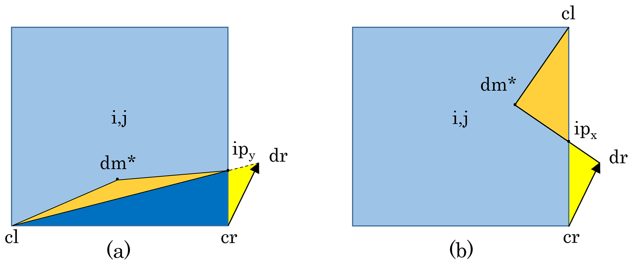
Figure C1 Schematic of departure regions on the south (a) and the east (b) edges of grid cell (i,j) (in light blue). The same code is used to calculate the departure region for both edges. To do so, the non-dimensional coordinate system is rotated by 90° for the east edge. This is why the corners for the east edge are also labeled as left (cl) and right (cr). The same convention applies to the departure points (dr). The orange triangles on both edges are defined by the EFA method by shifting the middle departure point to dm^*. The intersection point, ip_y, on the y axis for the south edge has non-dimensional coordinates (0,y_i), while ip_x for the east edge (on the rotated x axis) has non-dimensional coordinates (x_i,0).

On the east edge of cell (i,j), the orange triangle represents an area flux out of the cell, while the yellow triangle is an incoming flux. On the south edge, all three triangles represent outgoing fluxes. As a_n=0 in cell (i,j), the fluxes associated with the orange and the dark blue triangle are zero. The only triangles that matter are the yellow triangles associated with the south and the east edges. The triangle associated with the south edge has vertices cr, dr, ip_y, while the one associated with the east edge has vertices cr, dr, ip_x. In non-dimensional coordinates, the incoming area flux across the east edge is larger than the outgoing flux across the south edge. This should not lead to a negative net flux for cell (i,j). However, if the area factor, A_f, is different for the two yellow triangles, the outgoing area can exceed the incoming area, leading to negative ice area in cell (i,j).

As described in Sect. 5.1, the EFA method uses the cell area evaluated at the midpoint of the edge to calculate the non-dimensional area of the departure region. Both yellow and orange triangles in Fig. C1b therefore have $A_{\mathrm{f}}=A_E(i,j)$, where A_E(i,j) is the cell area evaluated at the E point. For the south edge, the dark blue and orange triangles have $A_{\mathrm{f}}=A_N(i,j-\mathrm{1})$ (Fig. C1a). Because the yellow triangle is not in the central region of the south edge, it is not part of the adjustment process. In the previous version of the remapping, the area factor assigned to this triangle was $A_{\mathrm{f}}=A_U(i,j-\mathrm{1})$. On highly deformed grids, $A_U(i,j-\mathrm{1})$ can be larger than A_E(i,j), resulting in negative fluxes.

To improve the robustness of the remapping for C-grid simulations, we modified the code by assigning the area factor A_E(i,j) to the yellow triangle associated with the south edge. Similar modifications are required for triangles referred to as TL (top-left), BL (bottom-left), TR (top-right), and BR (bottom-right) in the code. These modifications apply with or without the EFA method.

Differing area factors are less of an issue for the B-grid. Considering the same example, the departure region for the east edge would be defined by points cr, dr, and cl (Fig. C1b). The area flux into cell (i,j) would be much larger than the area flux out of the cell (yellow triangle in Fig. C1a), and there would be no negative fluxes.

We omit the details here, but a similar problem can arise with lone triangles (e.g., the yellow triangle in Fig. 4). This triangle is now assigned $A_{\mathrm{f}}=A_N(i,j)$ instead of A_U(i,j) as was done before, in the original code. All the lone triangles now use A_f at the center of the edge that they border.

As a result of the code modifications described above, another change was required to prevent negative areas. For simplicity, we omit the EFA triangles in this explanation; see Fig. C2. Here, we assume that the ocean cells (i,j), $(i-\mathrm{1},j)$, and $(i+\mathrm{1},j)$ do not have ice in category n. Moreover, there are ocean cells to the north, with a_n>0, while the southern boundary is a coastline (i.e., land cells). We look at the fluxes for category n.

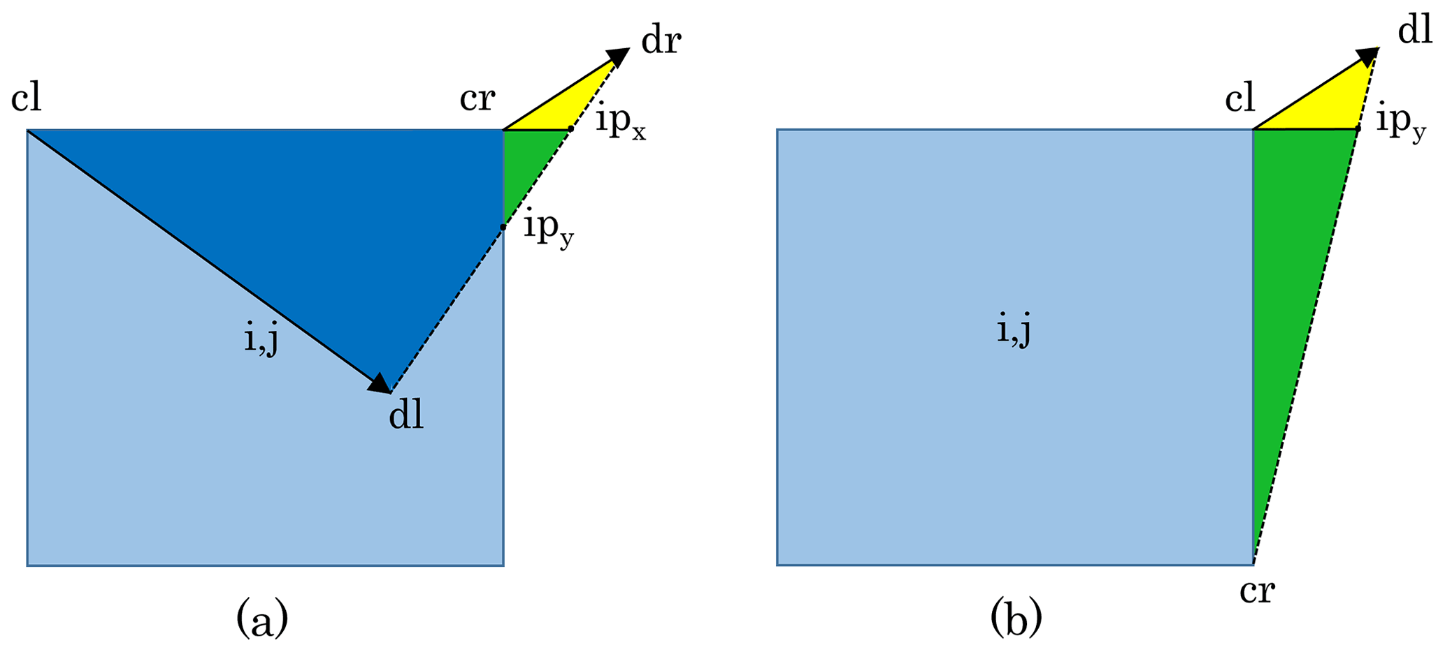
Figure C2 Schematic of departure regions on the north (a) and the east (b) edges of grid cell (i,j) (in light blue). The same code is used to calculate the departure region for both edges. To do so, the non-dimensional coordinate system is rotated by 90° for the east edge. The corners are labeled as left (cl) and right (cr). The departure points are dl and dr, and ip_x and ip_y are intersecting points on the x and y axes.

In rare situations, the segment joining dl and dr crosses two edges to form two corner triangles on the north edge of cell (i,j), as shown in Fig. C2a. Since a_n=0 in this cell, the departure region inside this cell associated with the north edge does not contribute to the total flux. This region, defined by the points cl, dl, ip_y, and cr, is shown in dark blue in Fig. C2a. Similarly, since a_n=0 in cell $(i+\mathrm{1},j)$, the green triangle for the north edge (Fig. C2a) and the green triangle for the east edge (Fig. C2b) do not contribute to the total flux. The two triangles that matter are the yellow ones. The one for the north edge, defined by cr, dr, ip_x, represents a flux out of cell (i,j), while the one for the east edge defined by cl, dl, ip_y corresponds to an incoming flux. In non-dimensional coordinates, the incoming area flux is greater than the outgoing flux. But if the two triangles have different area factors as described above, the net flux can be negative.

With the code changes described above, the yellow triangle for the east edge uses $A_{\mathrm{f}}=A_N(i+\mathrm{1},j)$. To ensure robustness (i.e., positive areas) with these changes, the code now uses $A_{\mathrm{f}}=A_N(i+\mathrm{1},j)$ for the yellow triangle associated with the north edge (Fig. C2a). This triangle is referred to as TR1 in the code. The green triangle, known as BR1, uses the area factor A_E(i,j). Similar modifications are required for the analogous TL1, BL2, and BR2 triangles.

Appendix D: C-grid analytical solution for a one-grid-cell-wide channel

We consider a uniform Cartesian grid with an east–west oriented one-grid-cell-wide channel by applying cyclic boundary conditions. The wind is constant and blows from the west. We further simplify the problem by assuming that the ocean is at rest and that the sea surface tilt term, the turning angle, and the Coriolis parameter are zero. The ice conditions are considered constant along the channel, with a being the concentration and $\stackrel{\mathrm{‾}}{h}$ the mean thickness. For this test, these fields do not change in time since transport, redistribution, and thermodynamics are turned off. Finally, we do not consider the plastic potential and simply set $e_G=e_F=e$. With these simplifications, v=0 and the u momentum equation becomes

$$\begin{array}{}\text{(D1)}& m{\displaystyle \frac{\partial u}{\partial t}}={\mathit{\tau }}_{\mathrm{a}}+{\mathit{\tau }}_{\mathrm{w}}+{\displaystyle \frac{\partial {\mathit{\sigma }}_{\mathrm{11}}}{\partial x}}+{\displaystyle \frac{\partial {\mathit{\sigma }}_{\mathrm{12}}}{\partial y}}.\end{array}$$

Because of the cyclic boundary conditions, $\frac{\partial {\mathit{\sigma }}_{\mathrm{11}}}{\partial x}=\mathrm{0}$. At steady state, the u momentum equation therefore becomes

$$\begin{array}{}\text{(D2)}& {\mathit{\tau }}_{\mathrm{a}}+{\mathit{\tau }}_{\mathrm{w}}+{\displaystyle \frac{\partial {\mathit{\sigma }}_{\mathrm{12}}}{\partial y}}=\mathrm{0}.\end{array}$$

Discretizing Eq. (D2) at the E point, we obtain

$$\begin{array}{}\text{(D3)}& {\mathit{\tau }}_{\mathrm{a}E}(i,j)+{\mathit{\tau }}_{\mathrm{w}E}(i,j)+{\displaystyle \frac{{\mathit{\sigma }}_{\mathrm{12}U}(i,j)-{\mathit{\sigma }}_{\mathrm{12}U}(i,j-\mathrm{1})}{\mathrm{\Delta }y}}=\mathrm{0}.\end{array}$$

At steady state, the shear stresses are given by

$$\begin{array}{}\text{(D4)}& {\mathit{\sigma }}_{\mathrm{12}}=\mathit{\eta }{D}_{\mathrm{s}},\end{array}$$

where $D_S=\partial u/\partial y$ because v is zero. Given the ellipse parameter e, η is expressed as

$$\begin{array}{}\text{(D5)}& \mathit{\eta }={\displaystyle \frac{e^{-\mathrm{2}}P}{\mathrm{2}{\mathrm{△}}^{*}}},\end{array}$$

where the capping formulation ${\mathrm{△}}^{*}=max[\mathrm{△},{\mathrm{△}}_{\min }]$ is used. Because ${\dot{\mathit{ϵ}}}_{\mathrm{11}}$ and ${\dot{\mathit{ϵ}}}_{\mathrm{22}}$ are zero, $\mathrm{△}=e^{-\mathrm{1}}\left|D_S\right|$.

With ${\mathit{\tau }}_{\mathrm{a}E}(i,j)=a{\mathit{\rho }}_{\mathrm{a}}{C}_{\mathrm{da}}{u}_{\mathrm{a}}^{\mathrm{2}}$ and ${\mathit{\tau }}_{\mathrm{w}E}(i,j)=-a{\mathit{\rho }}_{\mathrm{w}}{C}_{\mathrm{dw}}{u}_E^{\mathrm{2}}(i,j)$, Eq. (D3) can be written as

$$\begin{array}{}\text{(D6)}& \begin{array}{rl}& a{\mathit{\rho }}_{\mathrm{a}}{C}_{\mathrm{da}}{u}_{\mathrm{a}}^{\mathrm{2}}-a{\mathit{\rho }}_{\mathrm{w}}{C}_{\mathrm{dw}}{u}_E^{\mathrm{2}}(i,j)\\ & +{\displaystyle \frac{{\mathit{\eta }}_U(i,j)D_{\mathrm{s}U}(i,j)-{\mathit{\eta }}_U(i,j-\mathrm{1})D_{\mathrm{s}U}(i,j-\mathrm{1})}{\mathrm{\Delta }y}}=\mathrm{0},\end{array}\end{array}$$

where ρ_a is the air density, C_da the air drag coefficient, and u_a the surface wind velocity.

With the no-slip boundary condition, we can approximate the shear strain rate:

$$\begin{array}{}\text{(D7)}& {\displaystyle }{D}_{\mathrm{s}U}(i,j)={\displaystyle \frac{\mathrm{0}-u_E(i,j)}{\mathrm{\Delta }y/\mathrm{2}}},\text{(D8)}& {\displaystyle }{D}_{\mathrm{s}U}(i,j-\mathrm{1})={\displaystyle \frac{u_E(i,j)-\mathrm{0}}{\mathrm{\Delta }y/\mathrm{2}}},\end{array}$$

which means that $D_{\mathrm{s}U}(i,j)<\mathrm{0}$ and $D_{\mathrm{s}U}(i,j-\mathrm{1})=-D_{\mathrm{s}U}(i,j)$.

We want to solve Eq. (D6) for u_E(i,j). For simplicity, we drop (i,j) – that is, $u_E(i,j)=u_E$. With strong winds, the ice is in the plastic regime – that is, ${\mathrm{△}}^{*}=\mathrm{△}=e^{-\mathrm{1}}\left|D_{\mathrm{s}}\right|$. We can write Eq. (D6) as

$$\begin{array}{}\text{(D9)}& a{\mathit{\rho }}_{\mathrm{a}}{C}_{\mathrm{da}}{u}_{\mathrm{a}}^{\mathrm{2}}-a{\mathit{\rho }}_{\mathrm{w}}{C}_{\mathrm{dw}}{u}_E^{\mathrm{2}}-{\displaystyle \frac{P}{e\mathrm{\Delta }y}}=\mathrm{0}.\end{array}$$

The transition between the plastic and viscous regimes occurs for a wind velocity $u_{\mathrm{a}}=u_{\mathrm{a}*}$. At this transition, △=△_min, which leads to a sea ice velocity of $e{\mathrm{△}}_{\min }\mathrm{\Delta }y/\mathrm{2}$. Replacing u_E in Eq. (D9) by that expression gives

$$\begin{array}{}\text{(D10)}& a{\mathit{\rho }}_{\mathrm{a}}{C}_{\mathrm{da}}{u}_{\mathrm{a}*}^{\mathrm{2}}-a{\mathit{\rho }}_{\mathrm{w}}{C}_{\mathrm{dw}}{\left[{\displaystyle \frac{e{\mathrm{△}}_{\min }\mathrm{\Delta }y}{\mathrm{2}}}\right]}^{\mathrm{2}}-{\displaystyle \frac{P}{e\mathrm{\Delta }y}}=\mathrm{0}.\end{array}$$

Solving for u_a*, we get

$$\begin{array}{}\text{(D11)}& u_{\mathrm{a}*}={\left[{\displaystyle \frac{{\mathit{\rho }}_{\mathrm{w}}{C}_{\mathrm{dw}}}{{\mathit{\rho }}_{\mathrm{a}}{C}_{\mathrm{da}}}}{\left({\displaystyle \frac{e{\mathrm{△}}_{\min }\mathrm{\Delta }y}{\mathrm{2}}}\right)}^{\mathrm{2}}+{\displaystyle \frac{P}{a{\mathit{\rho }}_{\mathrm{a}}{C}_{\mathrm{da}}e\mathrm{\Delta }y}}\right]}^{\mathrm{1}/\mathrm{2}}.\end{array}$$

If $u_{\mathrm{a}}>u_{\mathrm{a}*}$, the ice is in the plastic regime and u_E can be found by solving Eq. (D9):

$$\begin{array}{}\text{(D12)}& u_E={\left[{\displaystyle \frac{{\mathit{\rho }}_{\mathrm{a}}{C}_{\mathrm{da}}{u}_{\mathrm{a}}^{\mathrm{2}}}{{\mathit{\rho }}_{\mathrm{w}}{C}_{\mathrm{dw}}}}-{\displaystyle \frac{P}{a{\mathit{\rho }}_{\mathrm{w}}{C}_{\mathrm{dw}}e\mathrm{\Delta }y}}\right]}^{\mathrm{1}/\mathrm{2}},\end{array}$$

where the first term is the free-drift velocity and the second term, which is there due to the rheology, slows down the ice. In the plastic regime, the shear stresses σ_12U(i,j) and ${\mathit{\sigma }}_{\mathrm{12}U}(i,j-\mathrm{1})$ are, respectively, $-e^{-\mathrm{1}}P/\mathrm{2}$ and $e^{-\mathrm{1}}P/\mathrm{2}$.

On the other hand, if the wind is weak (i.e, $u_{\mathrm{a}}<u_{\mathrm{a}*}$), the ice is in the viscous regime. In this case, ${\mathrm{△}}^{*}={\mathrm{△}}_{\min }$ and Eq. (D6) becomes

$$\begin{array}{}\text{(D13)}& a{\mathit{\rho }}_{\mathrm{a}}{C}_{\mathrm{da}}{u}_{\mathrm{a}}^{\mathrm{2}}-a{\mathit{\rho }}_{\mathrm{w}}{C}_{\mathrm{dw}}{u}_E^{\mathrm{2}}-{\displaystyle \frac{\mathrm{2}P{u}_E}{e^{\mathrm{2}}{\mathrm{△}}_{\min }\mathrm{\Delta }{y}^{\mathrm{2}}}}=\mathrm{0},\end{array}$$

which can be rewritten as

$$\begin{array}{}\text{(D14)}& u_E^{\mathrm{2}}+{\displaystyle \frac{\mathrm{2}P}{a{\mathit{\rho }}_{\mathrm{w}}{C}_{\mathrm{dw}}{e}^{\mathrm{2}}{\mathrm{△}}_{\min }\mathrm{\Delta }{y}^{\mathrm{2}}}}{u}_E-{\displaystyle \frac{{\mathit{\rho }}_{\mathrm{a}}{C}_{\mathrm{da}}{u}_{\mathrm{a}}^{\mathrm{2}}}{{\mathit{\rho }}_{\mathrm{w}}{C}_{\mathrm{dw}}}}=\mathrm{0}.\end{array}$$

The solution of Eq. (D14) is thus

$$\begin{array}{}\text{(D15)}& \begin{array}{rl}{u}_E& =-{\displaystyle \frac{P}{a{\mathit{\rho }}_{\mathrm{w}}{C}_{\mathrm{dw}}{e}^{\mathrm{2}}{\mathrm{△}}_{\min }\mathrm{\Delta }{y}^{\mathrm{2}}}}\\ & +\sqrt{{\left({\displaystyle \frac{P}{a{\mathit{\rho }}_{\mathrm{w}}{C}_{\mathrm{dw}}{e}^{\mathrm{2}}{\mathrm{△}}_{\min }\mathrm{\Delta }{y}^{\mathrm{2}}}}\right)}^{\mathrm{2}}+{\displaystyle \frac{{\mathit{\rho }}_{\mathrm{a}}{C}_{\mathrm{da}}{u}_{\mathrm{a}}^{\mathrm{2}}}{{\mathit{\rho }}_{\mathrm{w}}{C}_{\mathrm{dw}}}}}.\end{array}\end{array}$$