CICERO Simple Climate Model (CICERO-SCM v1.1.1) – an improved simple climate model with a parameter calibration tool

The CICERO Simple Climate Model (CICERO-SCM) is a lightweight, semi-empirical model of global climate. Here we present a new open-source Python port of the model for use in climate assessment and research. The new version of CICERO-SCM has the same scientific logic and functionality as the original Fortran version, but it is considerably more flexible and also open-source via GitHub. We describe the basic structure and improvements compared to the previous Fortran version, together with technical descriptions of the global thermal dynamics and carbon cycle components and the emission module, before presenting a range of standard figures demonstrating its application. A new parameter calibration tool is demonstrated to make an example calibrated parameter set to span and fit a simple target specification. CICERO-SCM is fully open-source and available through GitHub (https://github.com/ciceroOslo/ciceroscm, last access: 23 August 2024).

1 Introduction

Simple climate models (SCMs), also termed reduced-complexity models (RCMs), have an important role in climate modeling. While Earth system models (ESMs) are used to resolve climate processes on a resolved grid, they remain extremely resource-intensive; however, much simpler models can reproduce key globally aggregated outputs (e.g., globally averaged surface temperature) (Balaji et al., 2017; Schneider and Thompson, 1981; Wigley and Raper, 1992). Thus, simple models can be used to help understand and explain physical processes (e.g., Peters et al., 2011) or to be calibrated to replicate the behavior and uncertainty across a range of more complex ESMs (Meinshausen et al., 2011). SCMs can be used to estimate the climate uncertainties across thousands of emission scenarios in a short runtime (Kikstra et al., 2022), something which remains impossible for ESMs with today's computing power, and they have been used to quantify the uncertainty in key climate indicators such as climate sensitivity (Sherwood et al., 2020) and the remaining carbon budget(Lamboll et al., 2023).

Even though SCMs can be used to emulate more complex models, there is still value in maintaining a diversity of SCMs because the reduced-form representation of the climate often rests on a set of structural assumptions and modeling philosophies which limit the response of the model (Nicholls et al., 2021, 2020). SCMs can exhibit a wide range of complexity, ranging from simple one- or two-layer energy balance models which are used in the operational calculation of emission metrics (Aamaas et al., 2013) up to a more comprehensive representation of the carbon cycle and energy balance (e.g., Gasser et al., 2020; Meinshausen et al., 2011). There are also intermediate complexity models sitting somewhere between a SCM and an ESM, but for the purposes of this article, we consider SCMs to be models which allow the simulation of a scenario on a single CPU in seconds or shorter.

The different complexity levels of SCMs can lead to different outcomes when key physical processes are constrained from data, such as tradeoffs in climate forcers and carbon–climate feedbacks on different timescales, such that models with different structures constrained on the same data can exhibit different future constrained projection distributions (Jenkins et al., 2021; Kikstra et al., 2022; Lamboll et al., 2023). While SCMs can be calibrated to replicate the behavior of more complex models, there is also a variety of ways to do this. Calibration could be done only on the historical period using observational-based data (e.g., Aldrin et al., 2012) or on complex model simulations over longer time periods using scenarios (e.g., out to 2100; Meinshausen et al., 2011) or using idealized simulations (e.g., response to abrupt or gradual changes in CO₂ concentration) (Olivié and Stuber, 2010). Furthermore, different variables could be used in the calibration, such as concentrations, surface temperature, and ocean heat content (Smith et al., 2021b). Subjective calibration choices can also lead to differences in climate outcomes (Sanderson, 2020). Each level of model complexity and calibration method has advantages and disadvantages, and to ensure robust and policy relevant results, it is necessary to maintain and develop a range of SCMs.

The original version of the CICERO (Center for International Climate Research) Simple Climate Model (CICERO-SCM) was developed in 1999 (Fuglestvedt and Berntsen, 1999) to study the effects of future emissions on global mean surface temperature and sea level rise. Atmospheric carbon dioxide (CO₂) was estimated using an ocean mixed-layer pulse response function (Alfsen and Berntsen, 1999; Joos and Bruno, 1996). The response to other long-lived greenhouse gas emissions was estimated using simple first-order decay equations, and the radiative forcing was estimated using simple proportionality between concentration and forcing for each gas. Direct and indirect radiative forcing of aerosols and radiative forcing of tropospheric and stratospheric ozone (O₃) and stratospheric water vapor were implemented using simplified expressions. The total radiative forcing provided boundary conditions for an energy balance upwelling–diffusion ocean model (Schlesinger et al., 1992). A time-varying lifetime of methane (CH₄) was introduced after the IPCC (Intergovernmental Panel on Climate Change) Third Assessment Report and based on a linear interpolation of the changes in the hydroxyl radical (OH) concentration with CH₄ concentration, nitrogen oxides (NO_x), carbon monoxide (CO), and non-methane volatile organic carbon (NMVOC) emissions (Table 4.11, footnote b, in Ehhalt et al., 2001). Since then, the core structure of the CICERO-SCM has remained relatively unchanged, though the parameters have been constantly updated in line with the best-available science. The model has been used in a range of studies, such as historical contributions to global warming (den Elzen et al., 2005, 2013; Höhne et al., 2011; Skeie et al., 2017, 2021), global warming from different economic sectors (Skeie et al., 2009; Tronstad Lund et al., 2012), estimates of the climate sensitivity (Aldrin et al., 2012; Skeie et al., 2014, 2018), simple model intercomparisons (Nicholls et al., 2021, 2020), and an assessment of specific mitigation strategies (Myhre et al., 2011; Torvanger et al., 2012, 2013). The CICERO-SCM was also used in the IPCC Sixth Assessment Report (AR6) (Guivarch et al., 2022; Kikstra et al., 2022; Smith et al., 2021b).

In this article, we describe and assess an updated version of the CICERO-SCM, now written in Python and made openly accessible to encourage community development and engagement. The model has also been supplemented with features for parameter calibration and easier parallel runs.

2 Model structure

Figure 1 shows the overall structure and flow of the CICERO-SCM. The core of the model consists of one module, concentrations_emissions_handler.py (see Sect. 2.1), which calculates concentrations from emissions and forcing from concentrations or directly from emissions, and another module, upwelling_diffusion_model.py, which calculates temperature from forcing, using an upwelling diffusion energy balance model (UDM/EBM) (see Sect. 2.2). A main control module, ciceroscm.py, calls these two, transfers data from the emissions to the forcing module and then to the upwelling diffusion module, loops over years, and takes care of outputs. The model can be run directly from input concentrations or forcing time series, in addition to running all the way from emissions to temperatures. Inputs and outputs are all global and on a yearly time resolution (with some exceptions). The upwelling_diffusion_model.py has two hemispheres and does calculations using 12 sub-yearly time steps to ensure convergence. The forcing input is therefore for two hemispheres. Volcanic forcing input is on a monthly time resolution (see Sect. 2.2 and Appendix C for further details). The carbon cycle uses 24 sub-yearly time steps to integrate the carbon response; however, it inputs and outputs only yearly values (see Sect. 2.1.1). In Sect. 2.3 we describe the main differences between the new Python port version and the previous Fortran implementation.

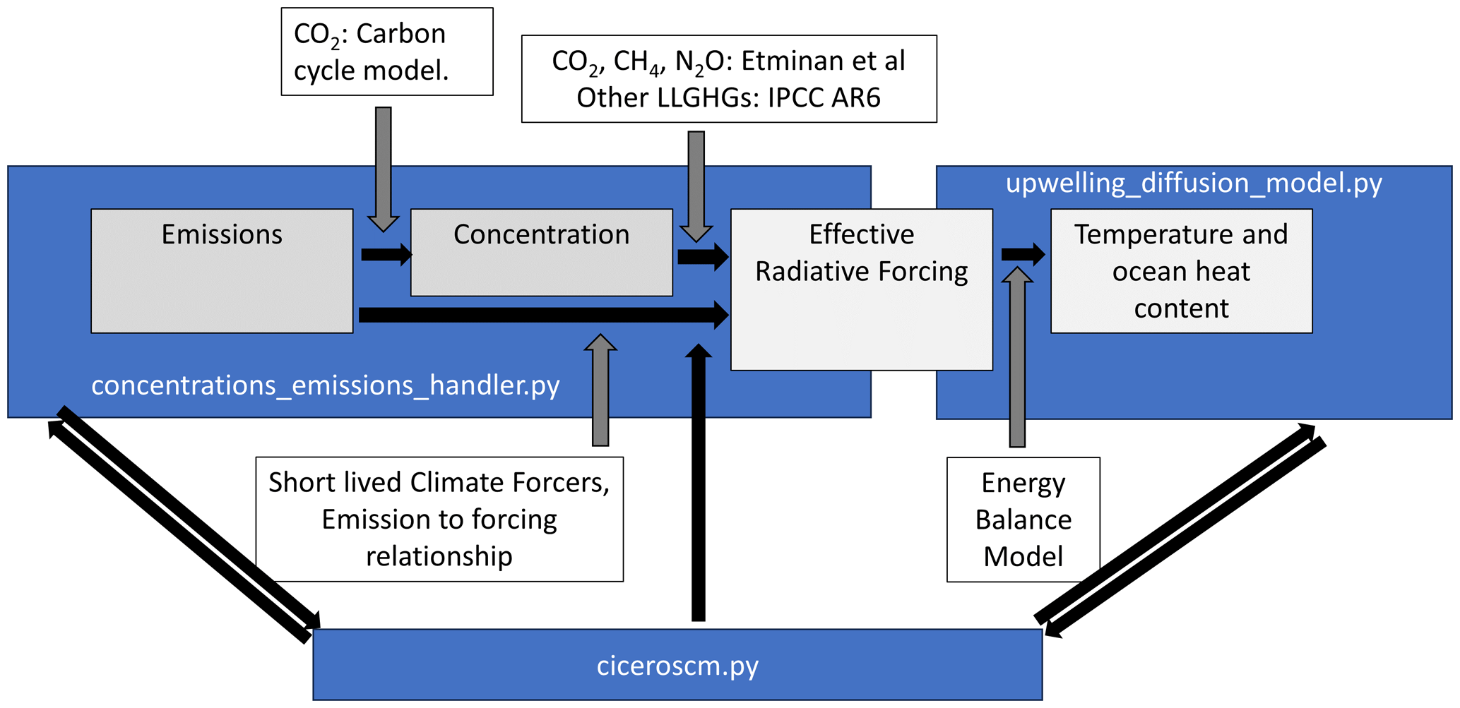
Figure 1 The core model structure. The concentrations_emissions_handler.py module calculates concentrations from emissions using a carbon cycle model for atmospheric CO₂ and first-order decay equations for other components. It then calculates forcing from concentrations using the Etminan et al. (2016) scheme for CO₂, CH₄, and N₂O and updated proportionality relationships for other gases. Simplified expressions calculate forcing directly from emissions for aerosols, O₃, and stratospheric water vapor. The effective radiative forcing is passed to the upwelling_diffusion_model.py, where it is used as input to the ocean energy balance model (Schlesinger et al., 1992) to calculate temperature and ocean heat content. This process is repeated for each time step, and looping and information passing is handled by the ciceroscm.py control module.

The code also includes various modules and help functions for handling perturbations (perturbations.py), handling utilities used by multiple modules (pub_utils.py and _utils.py), handling input in various formats (input_handler.py), and making default summary plots (make_plots.py). It also ships with a subpackage for handling parallel runs including a parallelization wrapper (cscmparwrapper.py), a module to define a distribution run (distributionrun.py), and modules to build and define a distribution and do calibration (_configdistro.py and calibrator.py). All of these tools will be described in more detail in Sect. 2.4.

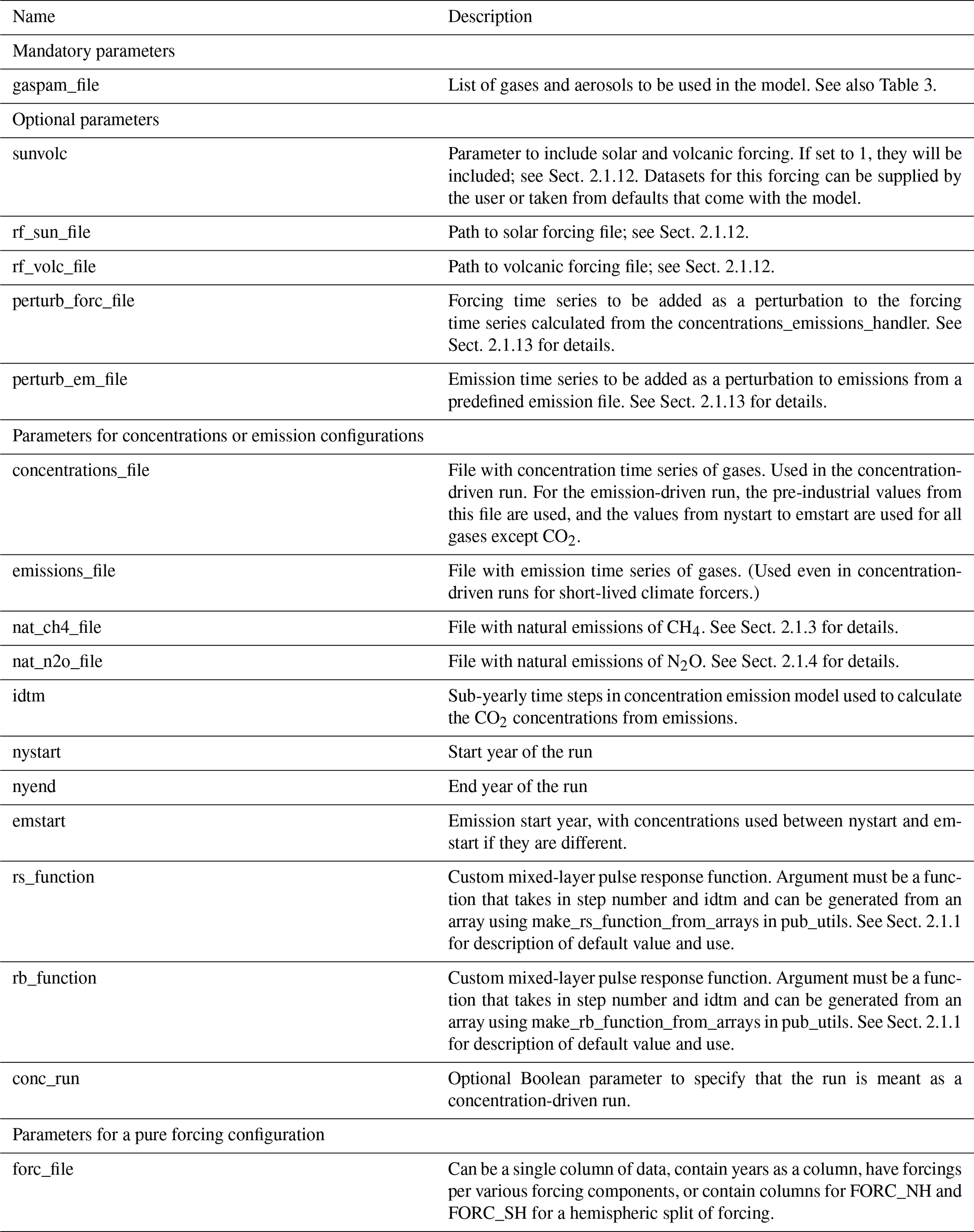
A regular run of the code will start by defining a CICERO-SCM instance that can then be used to run the model for the same experiment but with various parameter values. Table 1 shows the parameters for the creation of such an instance. A default run will lead to output files being generated, but the outputs can also be held in a dictionary with separate keys and corresponding values for outputs from the upwelling_diffusion_model.py and additional keys for datasets for the concentration, emissions, and forcing. A run can also produce automatic plots. Appendix A contains figures showing the automatic plots generated from a default configuration emission to forcing run of the CMIP6 historical experiment (Figs. A1–A11).

Table 1 Parameters used in defining a ciceroscm model object.

2.1 Emissions to radiative forcing – concentrations_emissions_handler

The module concentrations_emissions_handler.py calculates the effective radiative forcing time series. For each time step this is done by first calculating concentrations from emissions. In a concentration-driven run, this is done by simply reading the concentrations in. Otherwise, a carbon cycle described in Sect. 2.1.1 is employed to calculate the CO₂ concentrations, and a mass balance equation is used for the other components as described in Sect. 2.1.2, with special modifications to account for multiple decay processes and natural emission for CH₄ (Sect. 2.1.3) and nitrous oxide (N₂O) (Sect. 2.1.4). When concentrations have been calculated, forcing is derived. For this, the scheme described in Etminan et al. (2016) is first used to calculate the forcing from CO₂, CH₄, and N₂O (Sect. 2.1.5). Then looping over all other chemical components, forcing will be calculated using tabulated concentrations to forcing values (Sect. 2.1.6) or calculated specifically for various species (see Sect. 2.1.7 for tropospheric O₃, Sect. 2.1.8 for stratospheric O₃, Sect. 2.1.9 for stratospheric water vapor and for aerosol forcing, Sect. 2.1.10 for albedo from land use change, Sect. 2.1.11 for aerosol forcing, and Sect. 2.1.12 for solar and volcanic forcing).

Inputs to the module (Table 1) are files or datasets of emission and concentration time series (Table 1), a file or dataset to define what gases and substances to consider, and optional integers to define the start year, end year, year at which to start running from emissions, number of sub-yearly time steps for carbon cycle calculations, and a Boolean option to make the runs pure concentration runs. Additional optional parameters giving files or datasets for natural emissions of CH₄ and N₂O and custom pulse response functions for the carbon cycle model can also be passed.

Some concentration data are needed even in the emission-driven mode for pre-industrial concentrations and to define concentrations prior to the chosen year of emission start. The default year of the run start is 1750; the model uses CO₂ emissions from the outset, whereas non-CO₂ emissions start in the emission start year, with the default year in 1850, so up to the year of emission start, all other components have forcing calculated directly from concentrations. After the emission start, all components will have forcing calculated from emissions. Alternatively, the model can be configured to use prescribed concentrations for all gases for the duration of the run.

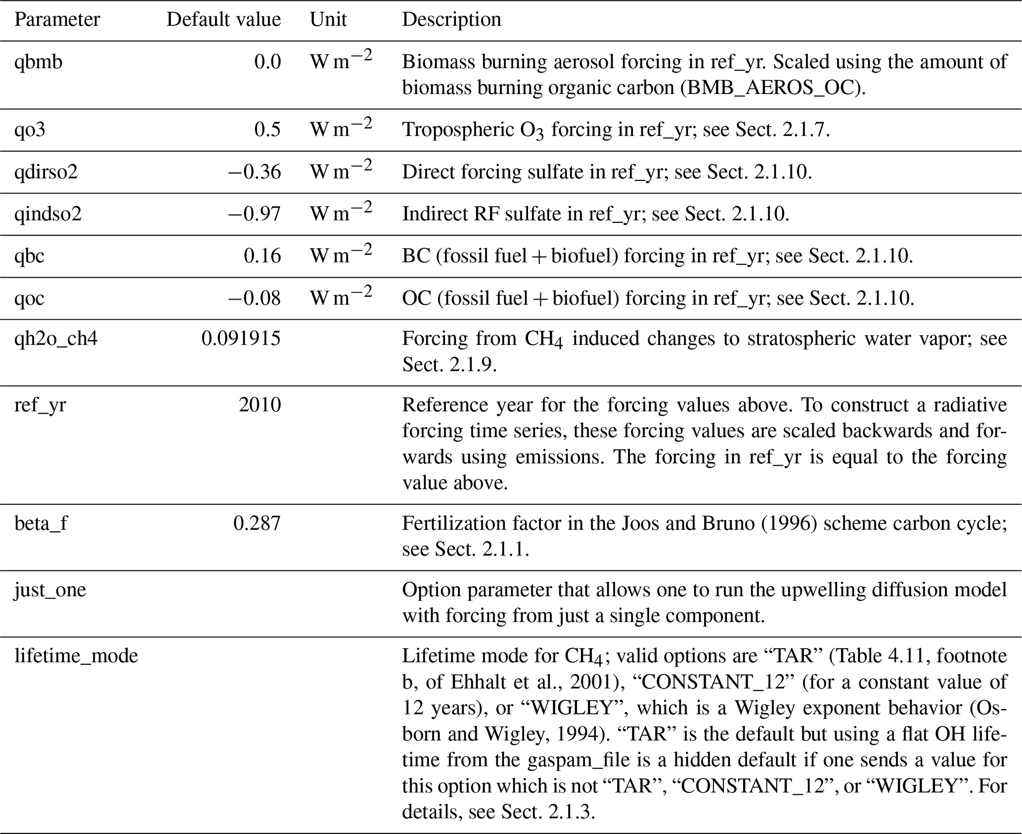
When the model is to be run, an array of parameters to control the properties of calculations can be adjusted. Table 2 shows these parameters, most of which control the forcing strength of various substances.

Table 2 Parameters for the concentration_emissions_handler.

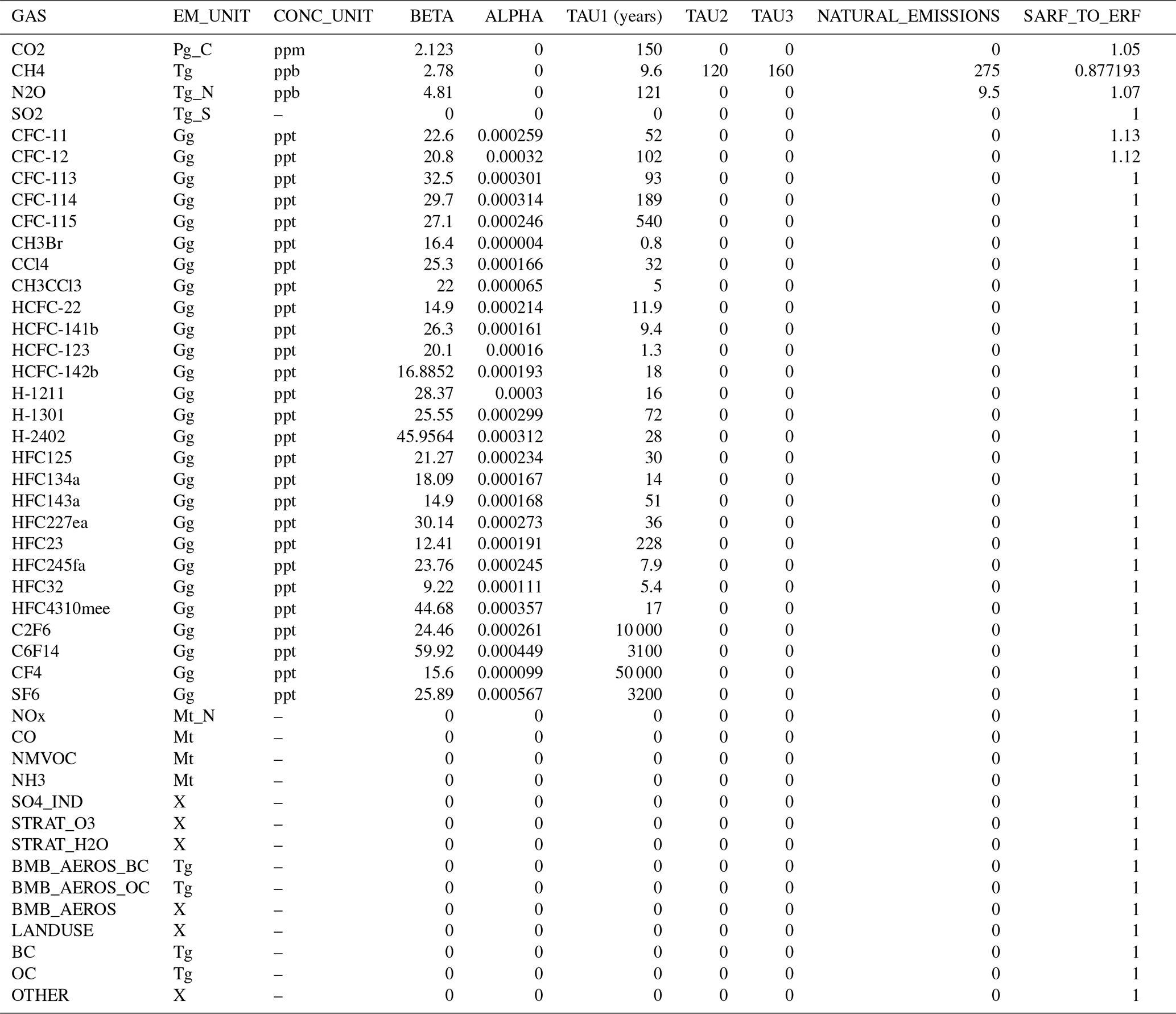
The gaspam_file or corresponding dataset defines which substances the model should consider and includes properties defining the calculations to be performed for them. Table 3 shows the default shipped gaspam_file and its structure. Information from this file is used in the calculations of both concentrations from emissions and when mapping concentrations to forcing.

Table 3 The structure of the gaspam_file. In it, properties of greenhouse gases and short-lived climate gases or precursors used in calculations are defined. This is the standard shipped version of the gaspam_file, but the user is free to define their own file that adds or subtracts gases and adjusts values for lifetimes, forcing strength, and so on as they see fit. The column headers are the names of the gas or substance in the run (GAS); the emission unit (EM_UNIT); the concentration unit (CONC_UNIT) in parts per million (m), billion (b), or trillion (t); the conversion unit between concentration and mass (unit is the ratio of the emission unit to the concentration unit) (BETA); the radiative efficiency (ALPHA) (in W m⁻² ppb⁻¹); and the lifetime in years. In the case of CH₄, the lifetime is split into the OH lifetime in years (TAU1), soil lifetime in years (TAU2), and stratospheric lifetime in years (TAU3). Also included are the natural emissions (NATURAL_EMISSIONS), where the unit should be the same as the emission unit, and a unitless conversion factor from stratospheric adjusted radiative forcing (SARF) to the effective radiative forcing (ERF) (SARF_TO_ERF). In the current implementation, TAU2 and TAU3 are only used for CH₄, and the ALPHA parameter is unused for CO₂, CH₄, N₂O, and aerosols. Gases with a dash (“–”) in the CONC_UNIT column are not converted from emissions to concentrations, and concentrations of these are not outputted or used in calculations. Gases with “X” in the emission column are not read from the emission files, but the forcing is calculated through other means from emissions of other components.

2.1.1 CO₂ – emissions to concentrations

The carbon cycle in the CICERO-SCM includes one part for the decay of CO₂ into the deep ocean and one part for impacts from the terrestrial ecosystem.

The deep-ocean sink is modeled using a scheme for CO₂ from Joos et al. (1996), and an explanation of the CICERO-SCM implementation can be found in Alfsen and Berntsen (1999). The CO₂ module uses an a diffusive air–sea exchange model combined with a decay function which represents the transfer of carbon to the deep ocean (Alfsen and Berntsen, 1999; Siegenthaler and Joos, 1992). Atmospheric CO₂ partial pressures δpCO_2,a(t) (in ppm) are calculated as follows:

$$\begin{array}{}\text{(1)}& \begin{array}{l}\frac{\mathrm{d}}{\mathrm{d}t}\mathit{\delta }p{\mathrm{CO}}_{\mathrm{2},\mathrm{a}}\left(t\right)=\frac{e\left(t\right)-f_{\mathrm{fer}}}{C_{\text{ppm\_to\_PgC}}}-A_{\mathrm{oc}}{f}_{\mathrm{a},\mathrm{s}},\end{array}\end{array}$$

where e(t) are the total emissions at time t (in PgC yr⁻¹), f_fer is the net carbon uptake of the terrestrial carbon cycle (PgC yr⁻¹), C_{ppm_to_PgC}=2.123 PgC ppm⁻¹ is a conversion factor between the partial atmospheric concentration of CO₂ and emitted petagrams of carbon. A_oc is the ocean area (in m²). f_a,s is the transfer rate between the ocean and atmosphere (in ppm yr⁻¹ m⁻²) represented as a function of the atmospheric and ocean carbon partial pressures as follows:

$$\begin{array}{}\text{(2)}& f_{\mathrm{a},\mathrm{s}}=k_{\mathrm{g}}\cdot \left[\mathit{\delta }p{\mathrm{CO}}_{\mathrm{2},\mathrm{a}}-\mathit{\delta }p{\mathrm{CO}}_{\mathrm{2},\mathrm{s}}\right],\end{array}$$

where k_g is the gas exchange coefficient ($k_{\mathrm{g}}=\frac{\mathrm{1}}{\mathrm{9.06}\cdot A_{\mathrm{oc}}}$ yr⁻¹), and δpCO_2,s is the partial pressure of the slab ocean, which is itself calculated as a function of the ocean temperature (T) and the carbon content of the mixed-layer (δΣCO₂(t)).

$$\begin{array}{}\text{(3)}& \mathit{\delta }p{\mathrm{CO}}_{(\mathrm{2},\mathrm{s})}=\mathrm{F}\left(\mathit{\delta }\mathrm{\Sigma }{\mathrm{CO}}_{\mathrm{2}}\left(t\right),T\right)\end{array}$$

F is the polynomial approximation given in Eq. (6b) in Joos et al. (1996). Though this equation could include temperature feedback to the carbon cycle, the CICERO-SCM does not currently include this, implementing instead a static T=18.2 °C, giving

$$\begin{array}{}\text{(4)}& \begin{array}{rl}F\left(x\right)& =\mathrm{1.3021}x+\mathrm{3.7929}\times {\mathrm{10}}^{-\mathrm{3}}{x}^{\mathrm{2}}+\mathrm{9.1193}\times {\mathrm{10}}^{-\mathrm{6}}{x}^{\mathrm{3}}\\ & +\mathrm{1.488}\times {\mathrm{10}}^{-\mathrm{8}}{x}^{\mathrm{4}}+\mathrm{1.2425}\times {\mathrm{10}}^{-\mathrm{10}}{x}^{\mathrm{5}}.\end{array}\end{array}$$

δΣCO₂ is calculated as a historical integral of past air–sea fluxes, f_a,s, modulated by a decay function, r_s, which represents transfer of carbon from the mixed layer to an (infinite) deep-ocean sink.

$$\begin{array}{}\text{(5)}& \mathit{\delta }\mathrm{\Sigma }{\mathrm{CO}}_{\mathrm{2}}\left(t\right)={\displaystyle \frac{c_{\mathrm{conv}}}{h}}{\int }_{t_{\mathrm{o}}}^t{f}_{\mathrm{a},\mathrm{s}}\left(t^{\prime }\right)r_{\mathrm{s}}\left(t-t^{\prime }\right)\mathrm{d}{t}^{\prime },\end{array}$$

where h is the height of the mixing layer in meters, c_conv=1.72210¹⁷ µmol m³ ppm⁻¹ kg⁻¹ is a conversion factor from the flux (from ppm to µmol) and seawater from volume (m³) to mass (kg). The function r_s is defined by two empirical decay functions, with the first for a period shorter than 2 years and the second empirical formulation for periods of 2 years or longer:

$$\begin{array}{}\text{(6)}& r_{\mathrm{s}}\left\{\begin{array}{ll}=\mathrm{0.12935}+\mathrm{0.21898}\cdot e^{-\frac{t}{\mathrm{0.034569}}}& \\ +\mathrm{0.17003}\cdot e^{-\frac{t}{\mathrm{0.26936}}}+\mathrm{0.24071}\cdot e^{-\frac{t}{\mathrm{0.96083}}}& \\ +\mathrm{0.24093}\cdot e^{-\frac{t}{\mathrm{4.9792}}}& \text{if}t<\mathrm{2.0},\\ =\mathrm{0.022936}+\mathrm{0.24278}\cdot e^{-\frac{t}{\mathrm{1.2679}}}& \\ +\mathrm{0.13963}\cdot e^{-\frac{t}{\mathrm{5.2528}}}+\mathrm{0.089318}\cdot e^{-\frac{t}{\mathrm{18.601}}}& \\ +\mathrm{0.03782}\cdot e^{-\frac{t}{\mathrm{68.736}}}+\mathrm{0.035549}\cdot e^{-\frac{t}{\mathrm{232.3}}}& \text{if}t\ge \mathrm{2.0},\end{array}\right.\end{array}$$

where t is measured in years.

Different versions of both r_s and the biotic decay function r_b, described below and with standard form according to Eq. (8), can be sent by sending a function as input when defining the concentrations_emissions_handler object according to Table 1.

The CICERO-SCM also includes the impacts of the terrestrial ecosystem, including CO₂ fertilization and the subsequent impact on the decay of biospheric material (Joos and Bruno, 1996). Net primary productivity is described as a function of the atmospheric CO₂ concentration, which modifies the emission time series directly, according to Eq. (1).

The carbon uptake of the terrestrial cycle f_fer is represented as

$$\begin{array}{}\text{(7)}& f_{\mathrm{fer}}\left(t\right)=\mathit{\delta }{f}_{\mathrm{npp}}\left(t\right)+{\int }_{-\mathrm{\infty }}^t\mathit{\delta }{f}_{\mathrm{npp}}\left(t^{\prime }\right)r_{\mathrm{b}}\left(t-t^{\prime }\right)\mathrm{d}{t}^{\prime },\end{array}$$

where δf_npp(t) is the instantaneous net primary productivity (NPP) from the current CO₂ concentration (in units of PgC yr⁻¹), and r_b is an impulse response function which represents the decay of the historically fertilized material produced during previous time steps:

$$\begin{array}{}\text{(8)}& \begin{array}{rl}{r}_{\mathrm{b}}& =\mathrm{0.70211}\cdot e^{-\mathrm{0.35}t}+\mathrm{13.4141}\times {\mathrm{10}}^{-\mathrm{3}}\cdot e^{-\frac{t}{\mathrm{20.0}}}\\ & -\mathrm{0.71846}\cdot e^{-\frac{\mathrm{55}t}{\mathrm{120.0}}}+\mathrm{2.9323}\times {\mathrm{10}}^{-\mathrm{3}}\cdot e^{-\frac{t}{\mathrm{100.0}}}.\end{array}\end{array}$$

The various terms represent the decay of ground vegetation, wood, detritus, and soil organic carbon, and time t is measured in years. δf_npp(t) is represented as a function of the atmospheric CO₂ concentrations:

$$\begin{array}{}\text{(9)}& \mathit{\delta }{f}_{\mathrm{npp}}\left(t\right)=f_{\mathrm{npp}}{\mathit{\beta }}_{\mathrm{f}}\ln \left({\displaystyle \frac{{\mathrm{CO}}_{\mathrm{2},\mathrm{a}}\left(t\right)}{\mathrm{278}\mathrm{ppm}}}\right),\end{array}$$

where f_npp is a measure of global terrestrial NPP (here taken as 60 PgC yr⁻¹; Atjay et al., 1979; Joos and Bruno, 1996), and CO_2,a(t) is the atmospheric concentration of CO₂ (measured in ppm). β_f (beta_f in the model and Table 2) is the “fertilization factor”.

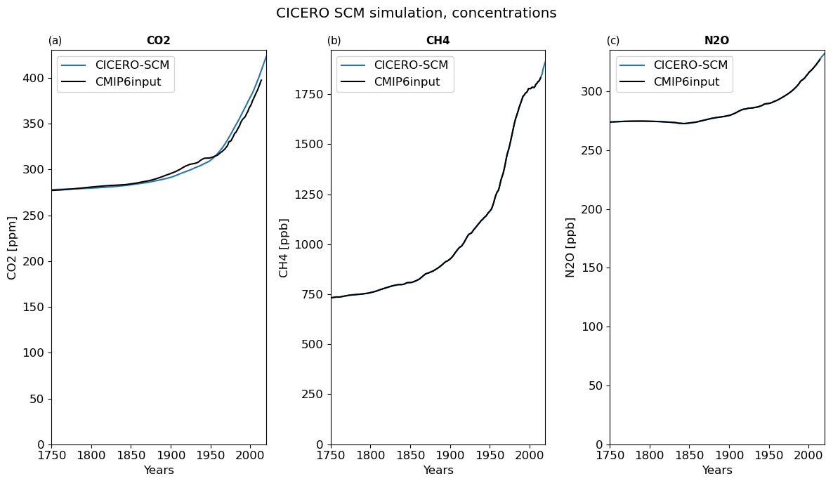
Figure 2 Calculated concentration of CO₂, CH₄, and N₂O from the CICERO-SCM from the CMIP6 emission time series (Meinshausen et al., 2017) compared to the concentrations of these gases prepared for CMIP6 (black line) from the same emission inputs (Meinshausen et al., 2017). Note that the natural emissions of CH₄ and N₂O are adjusted so that the calculated concentrations match the observational-based concentrations prepared for CMIP6.

Figure 2a shows the calculated concentrations of CO₂ from the CICERO-SCM using CO₂ emissions from Meinshausen et al. (2017, 2020). For reference, the CO₂ emissions in 2014 are split into 9.7 Pg carbon of fossil fuel emissions and 1.1 Pg carbon of land use change emissions.

2.1.2 Non-CO₂ component concentration calculations

The atmospheric concentration of non-CO₂ gases is determined by a mass balance equation,

$$\begin{array}{}\text{(10)}& {\displaystyle \frac{\mathrm{d}C}{\mathrm{d}t}}=P-Q\cdot C={\displaystyle \frac{E}{{\mathit{\beta }}_{\mathrm{gas}}}}-C\cdot {\displaystyle \frac{\mathrm{1}}{{\mathit{\tau }}_{\mathrm{gas}}}},\end{array}$$

where C is the concentration or mixing ratio of the gas (ppm and ppb), P is the production rate, and Q is the loss rate. The production, P, is given by the emissions per year, E, converted to mixing ratio units with β_gas, and τ_gas is the lifetime (in years). β_gas (BETA) and τ_gas (TAU1) are both gas-specific constants read from the gaspam_file (see Table 3). The production (emissions) is a function of time t (in years), E=E(t), while the loss rate (Q) is assumed to be constant, except for the case of CH₄ (see Sect. 2.1.3).

To solve this equation numerically, we use a first-order exponential integrator method. We first rearrange the equation as

$$\begin{array}{}\text{(11)}& {\displaystyle \frac{\mathrm{d}C\left(t\right)}{\mathrm{d}t}}+C\left(t\right)\cdot {\displaystyle \frac{\mathrm{1}}{{\mathit{\tau }}_{\mathrm{gas}}}}={\displaystyle \frac{E\left(t\right)}{{\mathit{\beta }}_{\mathrm{gas}}}},\end{array}$$

multiply both sides by $\exp \left(\frac{t}{{\mathit{\tau }}_{\mathrm{gas}}}\right)$, and combine

$$\begin{array}{}\text{(12)}& {\displaystyle \frac{\mathrm{d}}{\mathrm{d}t}}\left(C\left(t\right)\cdot \exp \left({\displaystyle \frac{t}{{\mathit{\tau }}_{\mathrm{gas}}}}\right)\right)={\displaystyle \frac{E\left(t\right)}{{\mathit{\beta }}_{\mathrm{gas}}}}\cdot \exp \left({\displaystyle \frac{t}{{\mathit{\tau }}_{\mathrm{gas}}}}\right).\end{array}$$

The emission (E) and mixing ratios (C) are annual, and we assume that they are constant over each 1-year period. This means that we can solve the equation exactly for each time step, t to t+Δt, where Δt=1 as the data is annualized. First, integrate both sides of the equation from t to t+1, noting that E(t) is constant between t+1 and t:

$$\begin{array}{}\text{(13)}& \begin{array}{rl}C& \left(t+\mathrm{1}\right)\cdot \exp \left({\displaystyle \frac{t+\mathrm{1}}{{\mathit{\tau }}_{\mathrm{gas}}}}\right)-C\left(t\right)\cdot \exp \left({\displaystyle \frac{t}{{\mathit{\tau }}_{\mathrm{gas}}}}\right)\\ & ={\displaystyle \frac{E\left(t\right){\mathit{\tau }}_{\mathrm{gas}}}{{\mathit{\beta }}_{\mathrm{gas}}}}\cdot \left[\exp \left({\displaystyle \frac{t+\mathrm{1}}{{\mathit{\tau }}_{\mathrm{gas}}}}\right)-\exp \left({\displaystyle \frac{t}{{\mathit{\tau }}_{\mathrm{gas}}}}\right)\right].\end{array}\end{array}$$

Then multiply both sides by $\exp \left(-\frac{t+\mathrm{1}}{{\mathit{\tau }}_{\mathrm{gas}}}\right)$, noting that $\exp \left(-\frac{t+\mathrm{1}}{{\mathit{\tau }}_{\mathrm{gas}}}\right)\cdot \exp \left(\frac{t}{{\mathit{\tau }}_{\mathrm{gas}}}\right)=\exp \left(-\frac{\mathrm{1}}{{\mathit{\tau }}_{\mathrm{gas}}}\right)$, which leads to

$$\begin{array}{}\text{(14)}& \begin{array}{rl}C(t+\mathrm{1})& =C\left(t\right)\exp \left(-{\displaystyle \frac{\mathrm{1}}{{\mathit{\tau }}_{\mathrm{gas}}}}\right)+{\displaystyle \frac{E\left(t\right){\mathit{\tau }}_{\mathrm{gas}}}{{\mathit{\beta }}_{\mathrm{gas}}}}\\ & \cdot \left[\mathrm{1}-\exp \left(-{\displaystyle \frac{\mathrm{1}}{{\mathit{\tau }}_{\mathrm{gas}}}}\right)\right].\end{array}\end{array}$$

This implementation is appropriate for discrete input data only, where the emissions (and concentrations) are assumed constant throughout the year. For a time step of shorter than 1 year, the emission (E) and mixing ratios (C) would need to have a resolution of under 1 year to match the time step. If working with emissions not assumed static over the sub-yearly timescale, then the original equation would be solved either analytically or using a numerical solution to the original differential equation (Aamaas et al., 2013). This version of the model only works for yearly data that follow this assumption.

Given this assumption, the method outlined here is an exact solution for each time step, utilizing the fact that emissions are constant in each time step. The solution can also be interpreted in terms of production and loss. The first term on the right-hand side represents the mixing ratio at the start of the time period (C_t), which decays according to the loss rate over 1 year. The second term on the right-hand side represents the emissions added in that year (E_t), which are assumed constant, and thus accumulate as sustained emissions over the year (Aamaas et al., 2013). At the end of the time period, C_t+1, the mixing ratio is thus the contribution from the material already in the atmosphere (first term) plus the contribution from material added to the atmosphere over the year (second term).

Several simplifications can help explain Eq. (14) and the unique characteristics of different non-CO₂ components. For a long-lived species, where τ≫1, such as N₂O, then the exponential term is close to one, and $C_{t+\mathrm{1}}\approx C_{\mathrm{t}}+\mathrm{\Delta }$, where Δ is a small contribution from new emissions. For a short-lived species, where τ≪1, such as sulfur dioxide (SO₂), then the exponential term is close to zero, and $C\left(t\right)\approx E\left(t\right)\cdot \frac{{\mathit{\tau }}_{\mathrm{gas}}}{{\mathit{\beta }}_{\mathrm{gas}}}$, showing that the mixing ratio is approximately a linear scaling of the emissions. And, in fact, for SO₂ and other aerosols, such a direct emission scaling is used to obtain forcing directly from emissions with no separate calculation of concentrations.

2.1.3 CH₄ – emissions to concentrations

The atmospheric concentration of CH₄ is determined by the mass balance equation (Eq. 14), leading to the solution and treatment as described above in Sect. 2.1.2. But for CH₄, the lifetime τ is not necessarily constant. The total lifetime is a combination of the lifetime with respect to OH (τ_OH), stratospheric lifetime (τ_strat) representing the chemical losses in stratosphere, and soil lifetime (τ_soil) representing the soil loss. The total lifetime and the individual lifetimes are related by $\frac{\mathrm{1}}{\mathit{\tau }}=\frac{\mathrm{1}}{{\mathit{\tau }}_{\mathrm{OH}}}+\frac{\mathrm{1}}{{\mathit{\tau }}_{\mathrm{soil}}}+\frac{\mathrm{1}}{{\mathit{\tau }}_{\mathrm{strat}}}$. The values of ${\mathit{\beta }}_{{\mathrm{CH}}_{\mathrm{4}}}$ (BETA), τ_OH (TAU1), τ_soil (TAU2), and τ_strat (TAU3) are specified in the gaspam_file (Table 3) with default values of 2.78 Tg CH₄ ppbv⁻¹ over 9.6, 120, and 160 years (Ehhalt et al., 2001) used. The total lifetime of CH₄ is 8.4 years.

The lifetime of CH₄ due to OH depends both on the CH₄ itself and emissions of NO_x, CO, and NMVOCs. CH₄ influences its own lifetime since the reaction between CH₄ and OH is also a significant loss reaction for OH. Increased emissions and higher atmospheric levels of CH₄ thus decrease the levels of OH. This will increase the chemical lifetime of CH₄, thereby further increasing the atmospheric levels of CH₄. CO and NMVOCs also have OH as a main loss reaction, and increased emissions of these components will decrease the levels of OH and increase the lifetime of CH₄. Enhanced levels of NO_x will work in the opposite direction as NO_x acts as a source of OH. Enhanced NO_x will increase OH and decrease the CH₄ levels.

Several parameterization options are available in the CICERO-SCM to deal with these effects on the CH₄ lifetime. The “lifetime_mode” can be set to the following in the pamset_emiconc (Table 2):

• “TAR” (default), where the τ_OH is adjusted following Ehhalt et al. (2001) (Table 4.11, footnote b). $\frac{\mathrm{1}}{\mathit{\tau }}=q=q\cdot \left(\mathrm{d}{\mathrm{lnC}}_{\mathrm{OH}}+\mathrm{1}\right)$, where

  $$\begin{array}{rl}\mathrm{d}\ln C_{\mathrm{OH}}& =-\mathrm{0.32}\cdot \left\{\ln \left[C_{{\mathrm{CH}}_{\mathrm{4}}}\left(\mathrm{year}\right)\right]-\ln \left[\mathrm{1751.0}\right]\right\}\\ & +\mathrm{0.0042}\cdot \left[E_{{\mathrm{NO}}_x}\left(\mathrm{year}\right)-E_{{\mathrm{NO}}_x}\left(\mathrm{2000}\right)\right]\\ & +\mathrm{0.000105}\cdot \left[E_{\mathrm{CO}}\left(\mathrm{year}\right)-E_{\mathrm{CO}}\left(\mathrm{2000}\right)\right]\\ & -\mathrm{0.000315}\cdot \left[E_{\mathrm{NMVOC}}\left(\mathrm{year}\right)-E_{\mathrm{NMVOC}}\left(\mathrm{2000}\right)\right].\end{array}$$

• “WIGLEY”, where ${\mathit{\tau }}_{\mathrm{OH}}={\mathit{\tau }}_{\mathrm{OH}}^{\mathrm{0}}\cdot {\left(\frac{C}{C_{\mathrm{0}}}\right)}^N$ and where C is the CH₄ concentration, C₀ is a reference CH₄ concentration of 1700 ppb, and the exponent N is 0.238 (Osborn and Wigley, 1994).

• “CONSTANT_12”, where τ_OH= 12.0.

If some other string is sent for this parameter, a flat lifetime from the gaspam_file is used. This flexibility in the OH lifetime options can allow the user to explore hypotheses and also allows the user to add and adapt a new OH lifetime scheme in a separate fork of the code without much effort.

There are also natural emissions of CH₄ which maintain a CH₄ concentration in the atmosphere in the absence of anthropogenic emissions (Saunois et al., 2020). To accurately represent the observed concentration, natural emissions of CH₄ can be precalculated (precalculate_natural_emissions.py in scripts/prescripts subfolder) with the same setup (lifetime mode and anthropogenic emissions), and these are added to E(t) before the calculation in Eq. (14). Further details on this can be found in Appendix B on the natural emissions of CH₄ and N₂O. Precalculated natural emission time series can be specified as an input file or input dataset (see Table 1). The model can also be run with fixed natural emissions specified in the gaspam_file (Table 3), and this is the model behavior when no data or files with natural emissions are sent and can also be used to provide constant natural emissions for other chemical components.

With the adjusted historical natural emissions of CH₄, the calculated CH₄ concentrations, by design, match observations of the CH₄ concentration (Fig. 2b). The model can also be run with fixed natural emissions specified in the gaspam_file (Table 3) and then the calculated concentration will give rise to discrepancies compared to observations due to the large uncertainties in the CH₄ budget terms (Saunois et al., 2020).

2.1.4 N₂O – emissions to concentrations

The atmospheric concentration of N₂O is determined by the same mass balance equation (Eq. 14) as for CH₄ but with a single constant lifetime of 109 years (Smith et al., 2021b), as specified in the gaspam_file (Table 3). The parameter ${\mathit{\beta }}_{{\mathrm{N}}_{\mathrm{2}}\mathrm{O}}$ (BETA) is given as 4.81 Tg[N] ppbv⁻¹, and hence, the emission input to the model is given in teragrams of nitrogen.

As for CH₄, the natural emissions can either be kept fixed with a value prescribed in the gaspam_file or sent as a precalculated file or dataset so that total (natural and anthropogenic) emission time series and the model setup will reproduce the historical concentration (Fig. 3c). For more on how natural emissions are estimated including assumptions for the future, see Appendix B on the natural emissions of CH₄ and N₂O.

2.1.5 CO₂, CH₄, and N₂O – concentrations to forcing

Based on the calculated concentrations, radiative forcing for CO₂, CH₄, and N₂O is calculated based on the simplified expressions in Table 1 of Etminan et al. (2016) that account for the overlap between the three components. The equations in Etminan et al. (2016) represent the radiative forcing that includes the adjustment to stratospheric temperatures (SARF). The initial concentrations of CO₂, CH₄, and N₂O used for the calculations are the concentration in the nystart year from the input file.

To include additional tropospheric adjustments, an adjustment factor can be specified in the gaspam_file (Table 3) to convert from SARF to effective radiative forcing (ERF) for each of the components. The default values in Table 3 are taken from the IPCC AR6, and the additional adjustments will increase the radiative forcing by 5 % for CO₂, decrease it by 14 % for CH₄, and increase it by 7 % for N₂O (Forster et al., 2021).

The calculated CO₂ ERF is less than the ERF time series from the IPCC AR6 (Forster et al., 2021), based on observed concentrations before 1950, and larger after 1950 (Fig. 3a). The reason for this is the under- and overestimation of the CO₂ concentration (Fig. 2a) and that 2xCO₂ ERF that is the effective forcing strength of a doubling of CO₂, based on Etminan et al. (2016), is stronger than the 2xCO₂ ERF in AR6, based on Meinshausen et al. (2020). The CH₄ ERF in Fig. 3b shows a reasonably good match. The N₂O ERF time series is in the lower range compared to the time series presented in IPCC AR6 (Forster et al., 2021). The difference can be explained by assuming a different pre-industrial concentration value in the run and by the fact that Forster et al. (2021) use a simplified expression, as used in Meinshausen et al. (2020), rather than the expressions from Etminan et al. (2016) used in CICERO-SCM.

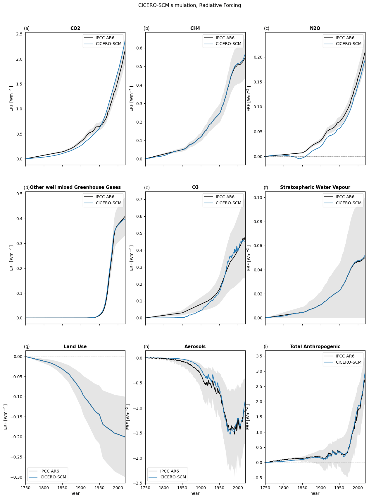
Figure 3 Calculated ERF from CICERO-SCM for selected components from 1750 to 2020. For comparison, the ERF time series from the IPCC and uncertainty ranges from this same dataset are also shown (Smith et al., 2021a, b). (a) CO₂, (b) CH₄, and (c) N₂O. (d) Other well-mixed greenhouse gases (GHGs) that are the sum of the contribution from CFC-11, CFC-12, CFC-113, CFC-114, CFC-115, CHBr, CCl₄, CH₃CCl₃, HCFC-22, HCFC-141b, HCFC-142b, C₂F₆, C₆F₁₄, CF₄, SF₆, HCFC-123, H-1211, H-1301, H-2402, HFC125, HFC134a, HFC143a, HFC227ea, HFC23, HFC245fa, HFC32, and HFC4310mee. (e) Total O₃ this is the sum of tropospheric and stratospheric O₃, (f) stratospheric water vapor, (g) land use (note that the CICERO-SCM uses the IPCC ERF time series as input), (h) total aerosol ERF, and (i) total anthropogenic forcing. Note the different scales on the y axis. Beyond 2014, the ssp245 future projections have been used as inputs.

2.1.6 Effective radiative forcing for other long-lived greenhouse gases

For the other long-lived or medium-lifetime greenhouse gases (such as CFCs (chlorofluorocarbons), HFCs (hydrofluorocarbons), and HCFCs (hydrochlorofluorocarbons)), the atmospheric concentrations are calculated based on the mass balance equation, emission time series, BETA values, and a single lifetime specified in the gaspam_file (Table 3) and as described in Sect. 2.1.2. The lifetimes are as in the IPCC AR6 WG1 (Table 7.SM.7 in Smith et al., 2021b).

For these components, radiative forcing is calculated based on a radiative efficiency (Table 7.SM.7 in Smith et al., 2021b),

$$\begin{array}{}\text{(15)}& \mathrm{SARF}=\mathrm{ALPHA}\cdot \left(C-C_{\mathrm{0}}\right),\end{array}$$

where ALPHA is read from the gaspam_file (Table 3), C is the concentration, and C₀ is the concentration in the nystart year. As most of these components are of anthropogenic origin, C₀ will be zero when starting from the pre-industrial era. Some components, however, have natural background concentrations. The pre-industrial concentrations are provided in the concentration file, and natural emissions are expected to be included for each year in the emission file; otherwise, a flat natural emission component can be specified in the gaspam_file.

Each component also has an option to include a conversion from SARF to ERF ($\mathrm{ERF}=\text{SARF\_TO\_ERF}\cdot \mathrm{SARF}$) to get the ERF that will be output and passed to the upwelling_diffusion_model.py.

In Forster et al. (2021), CFC11 and CFC12 have SARF to ERF adjustment factors of 13 % and 12 %, respectively. All other components have SARF to ERF factors of 1. However, different SARF to ERF conversion factors can be specified in the gaspam_file (see Table 3).

The calculated ERFs for the other GHGs compare well with the IPCC AR6 time series (Fig. 3d).

2.1.7 Tropospheric O₃

The tropospheric O₃ forcing is specified in the pamset_emiconc as qo3 (Table 2), and that is the radiative forcing in the reference year (ref_year) specified in the same parameter set. The default values are 0.5 W m⁻² in ref_year 2010, based on Smith et al. (2021b). The qo3 can include adjustments and be treated as ERF, or a factor converting SARF to ERF can be included in the gaspam_file (Table 3).

The time series of tropospheric O₃ forcing is calculated by combining the concentrations of CH₄ and emissions of NO_x, CO, and NMVOC, following Table 4.11, footnote b, of Ehhalt et al. (2001).

Assuming a tropospheric O₃ burden of 30 DU (Dobson units) in the reference year, the tropospheric O₃ burden is calculated as

$$\begin{array}{}\text{(16)}& \begin{array}{rl}{C}_{{\mathrm{O}}_{\mathrm{3}}}\left(t\right)& =\mathrm{30.0}+\mathrm{6.7}\cdot \left\{\ln \left[C_{{\mathrm{CH}}_{\mathrm{4}}}\left(t\right)\right]-\ln \left[C_{{\mathrm{CH}}_{\mathrm{4}}}\left(t_{\mathrm{ref}}\right)\right]\right\}\\ & +\mathrm{0.17}\cdot \left[E_{{\mathrm{NO}}_x}\left(t\right)-E_{{\mathrm{NO}}_x}\left(t_{\mathrm{ref}}\right)\right]+\mathrm{0.0014}\\ & \cdot \left[E_{\mathrm{CO}}\left(t\right)-E_{\mathrm{CO}}\left(t_{\mathrm{ref}}\right)\right]+\mathrm{0.0042}\\ & \cdot \left[E_{\mathrm{NMVOC}}\left(t\right)-E_{\mathrm{NMVOC}}\left(t_{\mathrm{ref}}\right)\right],\end{array}\end{array}$$

where C terms denote concentrations, E terms are emissions, t is time in years, and t_ref is the reference year. The default value for this is 2010.

The radiative forcing is calculated by scaling the qo3 (tropospheric ozone SARF in the reference year in W m⁻²) by changes in O₃ burden as follows:

$$\begin{array}{}\text{(17)}& \mathrm{SARF}=\mathrm{qo}\mathrm{3}\cdot {\displaystyle \frac{C_{{\mathrm{O}}_{\mathrm{3}}}\left(t\right)-C_{{\mathrm{O}}_{\mathrm{3}}}\left(t_{\mathrm{emstart}}\right)}{C_{{\mathrm{O}}_{\mathrm{3}}}\left(t_{\mathrm{ref}}\right)-C_{{\mathrm{O}}_{\mathrm{3}}}\left(t_{\mathrm{emstart}}\right)}},\end{array}$$

where t_emstart is the year when running with everything from the emission start.

Before the emission start, the forcing is scaled by fossil fuel CO₂ emissions, and t₀ is the first year of the run, i.e., nystart.

$$\begin{array}{}\text{(18)}& \mathrm{SARF}=\mathrm{qo}\mathrm{3}\cdot {\displaystyle \frac{E_{{\mathrm{CO}}_{\mathrm{2}}\mathrm{FF}}\left(t\right)-E_{{\mathrm{CO}}_{\mathrm{2}}\mathrm{FF}}\left(t_{\mathrm{0}}\right)}{E_{{\mathrm{CO}}_{\mathrm{2}}\mathrm{FF}}\left(t_{\mathrm{ref}}\right)-E_{{\mathrm{CO}}_{\mathrm{2}}\mathrm{FF}}\left(t_{\mathrm{0}}\right)}}\end{array}$$

Tropospheric O₃ is a short-lived component, and the global forcing is split into hemispheric forcing. The hemispheric weights for the global forcing is taken from the multi-model results in Skeie et al. (2020) and is 1.45 for the Northern Hemisphere and 0.55 for the Southern Hemisphere, as implemented in the routine calculate_hemispheric_forcing. The total O₃ forcing (tropospheric and stratospheric) is shown in Fig. 3d, and tropospheric O₃ ERF alone is shown in Fig. A8.

2.1.8 Stratospheric O₃

The loss in stratospheric O₃ is calculated from the concentration of chlorine- and bromine-containing components 3 years prior to the year in question to account for transport from the troposphere to the stratosphere and scaled by the number of chlorine or bromine atoms they contain.

$$\begin{array}{}\text{(19)}& \begin{array}{rl}\mathrm{SARF}& =-{\displaystyle \frac{\mathrm{0.287737}}{\mathrm{1000.0}}}\\ & \cdot \left[\mathrm{0.000552}\cdot \sum _i{\left(N_{{\mathrm{Cl}}_i}\cdot C_{{\mathrm{Cl}}_i}\left(t-\mathrm{3}\right)\right)}^{\mathrm{1.7}}\right.\\ & \left.+\mathrm{3.048}\cdot \sum _j{N}_{{\mathrm{Br}}_j}\cdot C_{{\mathrm{Br}}_j}\left(t-\mathrm{3}\right)\right],\end{array}\end{array}$$

where the sums run over the chlorine- and bromine-containing components, respectively; the C terms are concentrations (pptv – parts per trillion by volume) of each of these, the N terms are the numbers of chlorine or bromine atoms in each of them, and t is the time in years. The functional form is based on Appendix 2 of Harvey et al. (1997), and the scaling has been updated in line with Forster et al. (2007). This has been generalized a bit from the Fortran version, where the exact chlorine and bromine components considered were hard-coded rather than identified from the substances contained in the gaspam_file (Table 3).

The total O₃ ERF (tropospheric plus stratospheric) is shown in Fig. 3e and stratospheric O₃ separately in Fig. A8.

2.1.9 Stratospheric water vapor

CH₄ oxidized in the stratosphere produces water vapor. In the dry stratosphere, this additional water vapor will cause additional radiative forcing. The CH₄-induced stratospheric water vapor ERF is calculated by scaling the CH₄ ERF by a factor qh2o_ch4 specified in the pam_emiconc parameter set. The default value is 0.092, and that is 9.2 % of the CH₄ forcing in the reference year (Forster et al., 2021; Winterstein et al., 2019). The ERF time series for stratospheric water vapor is shown in Fig. 3f.

2.1.10 Albedo from land use change

The historical surface albedo land use change forcing used in the model is a prescribed forcing time series. The default time series used in the model is from IPCC AR6 (Forster et al., 2021; Smith et al., 2021b) and is extended for RCMIP (Nicholls et al., 2021, 2020). The ERF time series of this is shown in Fig. 3g, and beyond 2014, the albedo forcing projections for ssp245 are used.

The hemispheric split of forcing is based on the multi-model results from (Smith et al., 2020) and implemented in the routine calculate_hemispheric_forcing.

2.1.11 Aerosol effective radiative forcing

The ERF for the aerosol radiation interaction (ERFari) of sulfate, fossil fuel and biofuel (FFBF), black carbon (BC), organic carbon (OC), and biomass burning (BMB) aerosols are included in CICERO-SCM, and the aerosol forcing in ref_year (t_ref) for each aerosol component is specified in the pamset_emiconc (Table 2). The ERFari values in ref_yr are scaled by the corresponding historical emissions of SO₂, BC FFBF, OC FFBF, and biomass burning aerosols (BMB_AEROS).

The ERFari time series for individual aerosol components are shown in Fig. 4a. The total aerosol ERFari time series is shown in Fig. 4b and shows a good match with the IPCC AR6 time series.

$$\begin{array}{}\text{(20)}& E_{\mathrm{ref}}=E\left(t_{\mathrm{ref}}\right)-E\left(t_{\mathrm{0}}\right),\mathrm{ERF}=q_{\mathrm{aer}}{\displaystyle \frac{E\left(t\right)-E\left(t_{\mathrm{0}}\right)}{E_{\mathrm{ref}}}},\end{array}$$

where E(t) is the emissions of each aerosol species at time t in years, and q_aer is the forcing for this component in t_ref and is the tunable parameter (see Table 2) for each component.

The net ERF from biomass burning aerosols (BMB_AEROS) is calculated using the input BMB_AEROS_OC, as biomass burning emissions from OC and BC are assumed to be correlated and scaled according to Eq. (20) with the parameter qbmb. The default value of this parameter is 0, so the user needs to set it to a different value to include the effects of biomass burning aerosols.

The ERF for aerosol cloud interaction (ERFaci) in ref_year is linearly scaled with SO₂ emissions and calculated as ERFari, according to Eq. (20), as studies indicate that the total global effect is linear with SO₂ (Kretzschmar et al., 2017). The aerosol forcing components from a default run of the CICERO-SCM are shown in Fig. 4a. The split in the ERFari and ERFaci time series is show in Fig. 4b and compared to the IPCC AR6 results (Forster et al., 2021). ERFari follows the AR6 results quite closely, while ERFaci is not as close to the AR6 mean; however, the uncertainty range for this is very large.

The hemispheric split of aerosol forcing is based on multi-model results from Smith et al. (2020) and implemented in the routine calculate_hemispheric_forcing.

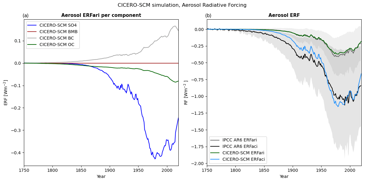
Figure 4 Panel (a) shows aerosol–radiation interaction forcing per aerosol component, and panel (b) shows the aerosol–cloud interaction and sum of aerosol–radiation interactions for all the components compared to AR6 results (Forster et al., 2021).

2.1.12 Solar and volcanic forcing

Solar forcing and volcanic forcing can be added as input time series. If the sunvolc parameter is set to 1, the model will either use user-defined files or datasets or use default files. The volcanic forcing series can be defined differently in each of the hemispheres and even with a monthly time resolution. Figure 5 shows default input time series of solar and volcanic forcing. These defaults are taken from Nicholls et al. (2021, 2020); however, for values beyond the year 2015, the following approximation has been made: solar forcing is assumed to be zero, whereas volcanic forcing is set to the mean forcing value in years 2006–2015.

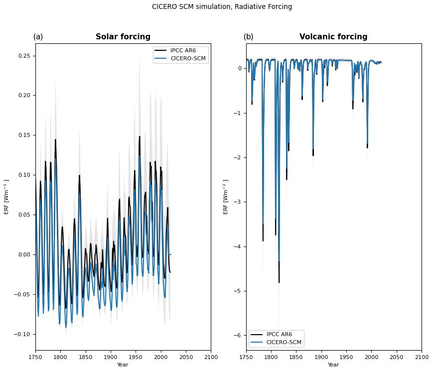
Figure 5 Default natural ERF time series for solar forcing (a) and volcanic forcing (b) used in the CICERO-SCM taken from RCMIP (Nicholls et al., 2021, 2020) compared to AR6 results (Forster et al., 2021; Smith et al., 2021b).

2.1.13 Perturbing forcing or emission time series

A common application of SCMs is to isolate and quantify the contributions to global radiative forcing and temperature change over time from individual anthropogenic emissions or sources, such as economic sectors. While there are different approaches to such an attribution (e.g., Boucher et al., 2021; Grewe, 2013), a well-established method is to have a perturbed case for which the emissions of interest are subtracted from a baseline case that includes all emissions. The attribution is thus the difference between the baseline case and the perturbed case (den Elzen et al., 2005; Fuglestvedt et al., 2008).

The CICERO SCM includes built-in options that enable this type of simulation, baseline, and perturbation. Specifically, two additional files can be input to the run, namely one that gives emission trajectories to be subtracted and one that gives the radiative forcing to be subtracted. The former is used in the case of the well-mixed greenhouse gases, while the radiative forcing perturbations are applied for the short-lived climate forcers.

In some cases, a given sector may affect climate through radiative forcing mechanisms that are not included in the SCM. A notable example is the formation of contrail cirrus from aviation emissions. It is possible to also include such ERF perturbations, which are then grouped in a category labeled “OTHER” and subtracted from the total net radiative forcing (RF) at the end of the concentration-to-forcing step of the model flow.

The time series of emissions and ERF to be extracted must be predefined in a specific format (sample files are provided in the open-source code base). If not directly available from more complex models, ERF time series are commonly derived by scaling the best-estimate present-day radiative efficiencies (i.e., ERF per unit emission) from available historical and/or future emission trajectories. For examples of how this has previously been done, including more chemically complex climate drivers such as NO_x-induced changes in O₃ and CH₄, see, e.g., Skeie et al. (2009).

2.2 Upwelling diffusion/energy balance model

To calculate the temperature change and storage of heat in the ocean as a response to the radiative forcing, an energy balance/upwelling diffusion model is used. The model is the hemispheric version (Schlesinger et al., 1992) of the global energy balance/upwelling diffusion model described in Schlesinger and Jiang (1990), and the structure of the model is shown in Fig. 6.

For each hemisphere, the ocean is subdivided into 40 vertical layers, where the uppermost ocean layer is the mixed layer. The ocean also has a polar region, where heat is transported from the mixed layer into the deep ocean and represents deep-water formation, i.e., sinking of cold water masses with relatively high salinity. Figure 6 shows the schematic ocean in the model.

The model is forced by hemispheric radiative forcing, and the climate response is governed by climate sensitivity, which is an explicit parameter in the model that takes the feedback processes in the climate system into account. The climate sensitivity parameter, λ (lambda), is the equilibrium climate sensitivity (defined as the equilibrium temperature response following a doubling of the CO₂ concentration) divided by the radiative forcing of a doubling of CO₂. Based on the formula in Etminan et al. (2016), SARF is 3.8 W m⁻² for a CO₂ doubling, and taking into account the adjustments of 5 % (Forster et al., 2021), the 2xCO₂ ERF is 4.0 W m⁻².

In each hemisphere, heat is exchanged between the atmosphere and the ocean in the upper mixed layer of the ocean. Heat is exchanged between each layer and the layers next to it via both diffusion and vertical upwelling advection and horizontally through interhemispheric heat exchange. Heat is also transported into the polar ocean in the mixed layer and back into the main ocean in the bottom most layer. This leads to a set of coupled differential equations which are solved by a mix of forward and backward implicit calculations to find the temperature change in each ocean layer. Equations are taken and implemented according to Appendix B in Schlesinger et al. (1992), the strengths of the various processes are defined by the parameters listed in Table 4, and the equations and their implementations are also detailed in Appendix C.

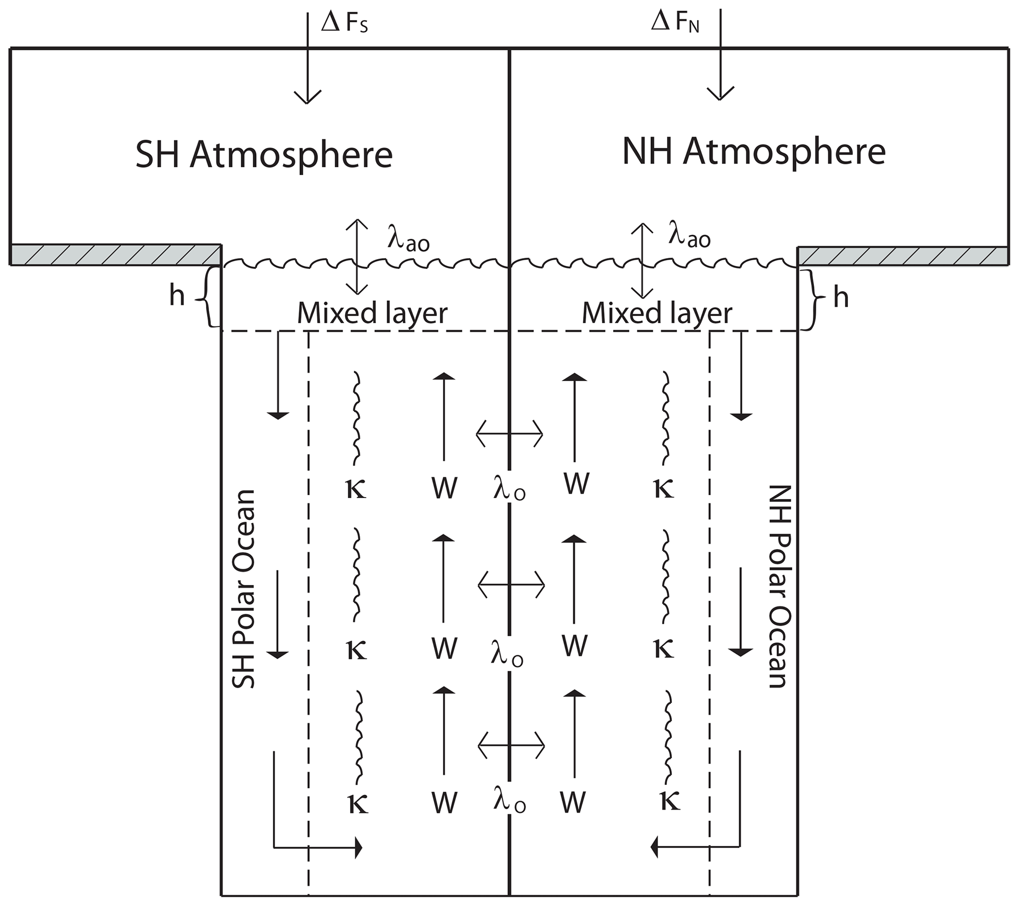
Figure 6 Redrawn from Schlesinger et al. (1992). The difference in the ocean and land fraction between Northern and Southern hemispheres is considered in the model but not illustrated in the figure.

Table 4 Description of pamset_udm, parameters in the energy balance/upwelling diffusion model with default values, units, and possible ranges.

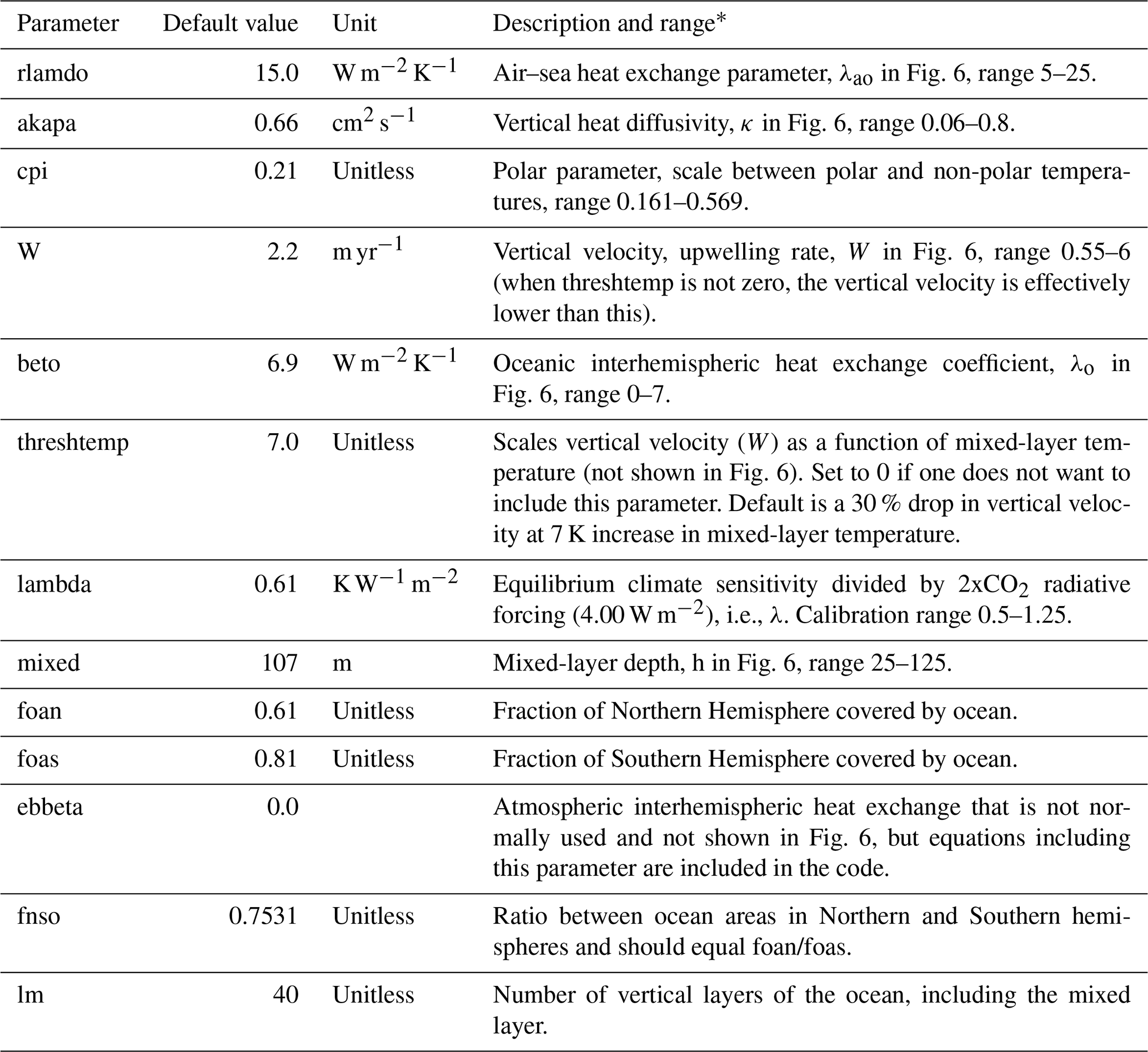
^* Ranges are taken from Aldrin et al. (2012), except the ranges for W and lambda, which are as used in the calibration run proof of concept in this article.

In addition to what is included in Schlesinger et al. (1992), the CICERO-SCM includes a threshtemp parameter, which changes the upwelling advection velocity depending on temperature, according to Raper et al. (2001). The parameter threshtemp is the temperature at which the upwelling velocity is reduced by 30 %. With threshtemp equal to 0, W will be constant, and this is a way of omitting the upwelling velocity dependency on temperature. Otherwise, the way that this parameter is scaled means that when $\mathrm{\Delta }T=\mathrm{10}/\mathrm{3}\cdot$ threshtemp, the advection will stop completely, and if the temperature surpasses this then that advection speed will become negative.

The temperature changes in the ocean layer calculated in the energy balance/upwelling diffusion model are finally used to calculate values for the ocean heat content (OHC) and ocean heat content of the uppermost 700 m (OHC700). For each hemisphere, separately and as a global average of the two, it is used to calculate the three temperature quantities: T_air, which is the global surface air temperature (GSAT); T_sea, which is the global sea surface temperature; and T_blended, which is the combined quantity calculated from the mixed-layer ocean temperature over the ocean and atmospheric temperature over land (global mean surface temperature – GMST). Finally, hemispheric and global averages for the radiative imbalance (RIB) are obtained. All these quantities are derived from calculations of the temperature T_l in the 40 layers of the ocean for each month of the year.

The temperature values are calculated from the ocean mixed-layer temperature T_l according to

$$\begin{array}{}\text{(21)}& \begin{array}{rl}{T}_{\mathrm{sea}}& ={\stackrel{\mathrm{‾}}{T}}_{\mathrm{l}},T_{\mathrm{air}}={\displaystyle \frac{\stackrel{\mathrm{‾}}{q+f_{\mathrm{ocean}}\cdot {\mathit{\lambda }}_{\mathrm{ao}}\cdot T_{\mathrm{l}}}}{\frac{\mathrm{1}}{\mathit{\lambda }}+f_{\mathrm{ocean}}\cdot {\mathit{\lambda }}_{\mathrm{ao}}}},\\ & T_{\mathrm{blended}}=\stackrel{\mathrm{‾}}{f_{\mathrm{ocean}}\cdot T_{\mathrm{sea}}+\left(\mathrm{1}-f_{\mathrm{ocean}}\right)\cdot T_{\mathrm{air}}},\end{array}\end{array}$$

where means are taken over 12 sub-yearly time steps; q is the mean forcing over the preceding year (in W m⁻²); f_ocean is the ocean fraction in the area under consideration (Northern Hemisphere, Southern Hemisphere, or global); λ_ao and λ are the tunable parameters of rlamdo and lambda, respectively (see Table 4 for details and units); and T_l is the temperature in uppermost ocean layer i.e., in the mixed layer.

The radiative imbalance (RIB) and ocean heat content (OHC) are similarly derived according to

$$\begin{array}{}\text{(22)}& \begin{array}{rl}\mathrm{RIB}& =\mathrm{ERF}-{\displaystyle \frac{T_{\mathrm{blended}}}{\mathit{\lambda }}},\mathrm{OHC}=\sum _{l=\mathrm{1}}^{\mathrm{maxdepth}}\mathit{\rho }\cdot c_p\\ & \cdot A_{\mathrm{Earth}}\cdot z_{\mathrm{l}}\cdot T_{\mathrm{l}}\cdot f_{\mathrm{ocean}},\end{array}\end{array}$$

where ρ is the density of seawater (assumed here to be constant at 1030 kg m⁻³), c_p is the specific heat capacity of seawater (3.997×10³ J kg⁻¹ K⁻¹), A_Earth is the surface area of the Earth (in m²), and z_l is the height of the layer in meters. The sum goes over all the layers of the ocean either down to 700 m, in which case the last layer is only a fractional layer, or all the way down, depending on whether the calculation is for OHC down to 700 m or for total OHC. In practice, the ocean heat content in each hemisphere is added together for each layer in the sum; hence, the area used, A_Earth, is rather the area of a hemisphere (2.55×10¹⁴ m²).

2.3 Model differences between new Python version and old Fortran version

The Python version is overall quite faithful to the previous Fortran version (at least it is possible to run it quite comparably). However, the Python version has more flexibility in what can be changed using parameters rather than what is hard-coded. For instance, the addition of SARF_TO_ERF parameters in the gaspam_file is a new addition, as is the option to run for different sets of years not starting in 1750, and many new tunable parameters have been added. In the Fortran version, one could tune the parameters lambda, akapa, cpi, W, rlamdo, beto, mixed, qbmb, qdirso2, qindso2, qbc, qoc, and qo3 using a parameter file needed for every run. In the Python version, one can also tune threshtemp, qh2o_ch4, and beta_f. One can also change parameters like the reference year and the ocean fractions in each hemisphere (foan and foas). One can also choose and even tune the functional forms for the carbon mixed-layer pulse response function (Eq. 5) and the biotic decay function (Eq. 8). With the Python version, swapping between emission- or concentration-driven runs or simply accessing functions from the code is much easier than it was in the Fortran version, where such changes required producing a new compiled executable from a modified version of the code. Since the code is openly available and more readable, a user can also much more easily change some part of the code to make even more parameters tunable or even swap out some of the modules and run the model, for instance, with a simplified energy balance model. In addition, the model can be run with both file and dataset inputs, and the functionality for reading from files or handling dataset inputs is separated from the main code.

The Python code is also fully open and can be included as a regular Python package using pip. It includes automatic tests, including a regression test, to make sure the results from the energy balance model can be directly comparable to the previous version, and the emission-to-forcing part can be comparable enough (this part of the calculation includes quite a lot of subtractions of nearly equal numbers, which means the comparison is less direct between the two versions). The regression tests directly compare the energy balance output from the Fortran version to check that when given the same forcing input, temperatures and ocean heat content are the same up to a relative error of less than 1 % throughout the run for a few different forcing scenarios (including a single-year forcing change, a 1 % increase in CO₂ per year of the experiment, and running with and without volcanic and solar forcing). The modeling flow from concentrations from to forcing and temperature is tested in a similar way, using a typical historical run, but when going all the way from emissions, the beginning of the run involves small values calculated by subtracting numbers of very similar size from each other, meaning that rounding differences become important; hence, we only require regression up to 1 % for a couple of years for the test to pass.

The code also includes plotting capabilities and tools for distribution runs and calibration which we will describe in further detail below. The automatic plots generated include time series plots of ocean heat content, radiative imbalance, temperature, and component-separated plots for emissions, concentrations, and radiative forcing. Examples of these plots for a historical run using all default parameters are included in Appendix A.

With the publicly available Python version on GitHub, there are also various example scripts to show usage, as well as scripts to prepare natural emission files for CH₄ and N₂O and perturbation files. Automatically generated documentation for the code, as well as a descriptive readme file to describe usage, is also included.

Currently, the code is somewhat slower than the original Fortran code was. A standard run from 1750 to 2100 from emissions to concentrations with the Fortran version usually takes under half a second, whereas the updated code takes around 3 s to do the same. This is a point for future improvement; however, the readability is considerably improved.

Figure 7 shows how the temperature output from the same parameter distributions used in the AR6 process results compares when run in the new version and the original Fortran version. Both the new Python version and the original Fortran version are included in the openscm runner (Nicholls et al., 2021). Clearly, the results are not very different between the two versions.

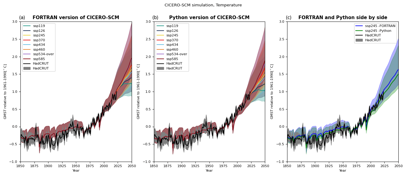
Figure 7 This figure shows the GMST from the ensemble used for the AR6 report (Kikstra et al., 2022; Smith et al., 2021b), as run with the current updated version and the old Fortran version panel (a) and in the new Python version panel (b), compared to observations from the observational dataset HadCRUT (Morice et al., 2021). In panel (c), for easier comparison, only the results for ssp245 are shown for both the Fortran version (in blue) and the Python version (in green). The comparison between the plots mainly shows that the ported Python version reproduces the old results quite faithfully when given the same parameter set, although there are some changes that generally make the Fortran version results a bit warmer than the Python version when given exactly the same parameters.

2.4 New parallel and calibration tools

Additions to the Python version are integrated parallelization and calibration tools. These include the options to run over a parameter distribution set defined in a JSON file or over multiple scenarios in parallel or some combination of both.

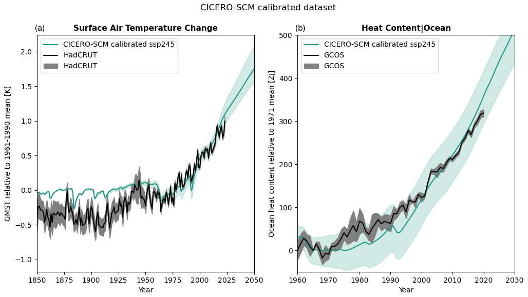
Figure 8 Results from a 100-member ensemble calibrating qindso2, W, and lambda to fit observed temperature from HadCRUT (Morice et al., 2021) and total ocean heat content from the Global Climate Observing System (GCOS) (von Schuckmann et al., 2023a). Panel (a) shows the temperature for the 2.5th to the 97.5th percentile compared to the same in the HadCRUT dataset. Panel (b) shows the ocean heat content for the 5th to 90th percentile compared to the same in GCOS. GMST (surface air temperature change) is shown as the change relative to the 1961–1990 period, while the ocean heat content is shown relative to 1971 ensemble mean values.

The parameter distribution may also be generated using the calibration tools; these can both simply be used to produce either Latin hypercubes or Gaussian distributions of a given size over any subset of the tunable parameters to be run over directly or saved as a JSON file for later use, or they can be used to tune parameters over such a prior distribution to fit the distribution of one or more output parameters, resulting in a tuned parameter ensemble to be run over and saved in a JSON file for later use.

The calibrator tool fits a set of n samples to distribution functions for some subset of the parameters. The priors over the distribution space can be Gaussian distributions or Latin hypercubes, and sampling is continued until a distribution of the required size is found. Samples are generated according to the prior and run in parallel chunks. Samples are then saved or rejected, according to the calibration distribution over some outputs. In practice, this is done by comparing its placement in the distribution for each variable to a random number and keeping samples that are placed closer to the mean than the random number. Be aware that the larger the calibration space, i.e., the dimensionality (number of parameters) and range of the prior parameter distribution, and the higher the number of data points to fit to, the higher the fraction of rejection and the higher the number of chosen samples needed to get a good fit. There is also a tunable cap on the total sampling to avoid infinite looping. With non-informative priors, the calibration might also need to be run for very many loops to get the required number of samples. Since quite a few of the parameters are independent, relating to specific components and diagnostics, a less computationally intensive calibration workflow might be tuning only a small subset of parameters separately to various outputs at a time. For instance, carbon cycle parameters can first be tuned to reproduce a CO₂ concentration time series, before the tuning forcing and climate sensitivity or other energy balance model parameters, to get the observed ocean heat content and temperature change distributions. Below, we demonstrate how the calibration can be used to get a parameter distribution.

As a proof of concept, we have produced 100-member ensemble of parameter sets, calibrating the parameters W (vertical velocity) and lambda (the climate sensitivity parameter) from the pamset_udm and qindso2 (ERFaci in ref_year) from the pamset_emiconc, keeping all other parameters at default values. Parameter ranges were 0.55–6, 0.5–1.25, and −1.75 to −0.25, respectively. The calibration was made to fit the observed temperatures from HadCRUT (Morice et al., 2021) and ocean heat content from GCOS (von Schuckmann et al., 2023a) time series, including uncertainties. However, in order to not make the fit too difficult for a quick demonstration, only data from every 30th year of the time series were used. Other approaches to the calibration could be fitting the overall RMSE between data and observations for the whole time series or fitting the mean difference in time windows. For an even better fit, more of the data should be used, more parameters might need to get fitted, and a larger ensemble should be constructed. Uncertainties that cannot be modeled with this setup still include input data uncertainty. The aerosol forcing calibration in this model can also only scale the aerosol forcing overall and not span uncertainties in its overall time evolution. Figure 8 shows how the 100-member calibrated set compares to the observational datasets in practice.

3 Conclusions

In this paper, we have described the CICERO-SCM simple climate model in its current incarnation as a Python-implemented open-source model. Though the model has been improved in terms of readability and user-friendliness, opportunities for further development abound. There are also many questions that the model is not currently suited to answer for which it could be adapted to answer.

In terms of technical modifications, the Python version is still slower than the Fortran model, and opportunities for further speed-ups should be explored. A fair bit of time could likely be shaved off the runtime through using more efficient data structures and calculations. However, such modifications may also come at the expense of the readability or easy model adaptation to new usages. Making the calibration more efficient, flexible, and statistically robust is also a technical priority. Eventually producing and updating the calibrated parameter sets that represent good fits to current available knowledge form the end goal of such an exercise. Keeping the model up to date with libraries and packages should also be a part of the development moving forward.

As for the functionality, the current modular structure allows for parts of the model to be used independently and provides options to change the emissions to a forcing or energy balance model with different models altogether. This could allow for testing and updating, for instance, using a more efficient ocean model with fewer layers or having a simpler, faster, and less readable emission to forcing module which can be interchanged with the current more readable and adaptable, yet slower, version. However, we acknowledge that modularity could be improved further – for example, through isolating the carbon cycle module.

Some updates that could open up the exploration of questions that the model currently does not answer properly include, but are not limited to, the regionalization of the temperature response; the inclusion of temperature feedbacks into the carbon uptake; a component breakdown of the carbon cycle to keep track of the carbon amounts in the various pools (representing processes which impact both heat and carbon transport in the ocean, for example); a more proper treatment of aerosol–cloud interactions to account for time delays in cloud formation (Jia and Quaas, 2023); the inclusion of nitrate aerosols, updated formulas for O₃ ERF, and updated CH₄ lifetime treatments reproducing more recent atmospheric chemistry model results (Skeie et al., 2023; Stevenson et al., 2020); continuous updates of lifetimes and forcing strength for various compounds; the inclusion of more compounds thought to have a climate impact in the future such as, for instance, molecular hydrogen (Hauglustaine et al., 2022; Paulot et al., 2021; Sand et al., 2023; Warwick et al., 2023) or ammonia (NH₃) (Bertagni et al., 2023).

In general, we hope that this open-source and accessible version of the model will facilitate expanded use and community development of the model, and we hope to see colleagues and users engage with it in whatever way they find most useful.

Appendix A: Default plots from a run with all parameters set to default values

The module includes automatic plotting options. Using these options, we can plot the time evolution of emissions, concentrations, and forcing changes per component, as well as ocean heat content change, radiative imbalance, and temperature change. Below, such plots from a run with all parameter values set to default values and run with the historical CMIP6 input data are shown.

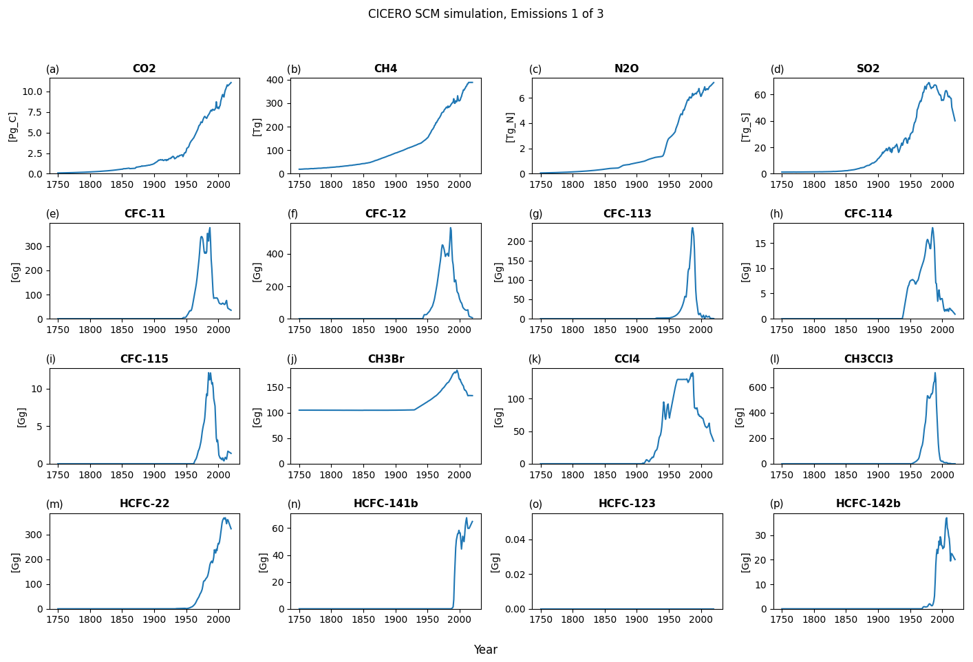
Figure A1 Default emission output plot number 1 for a run with default parameters using historical emissions up to 2014 and the ssp245 emission year 2014 to the end of the year 2020 – all from RCMIP (Nicholls et al., 2020). The input dataset did not include data for HCFC-123; hence, the value for this gas is zero throughout.

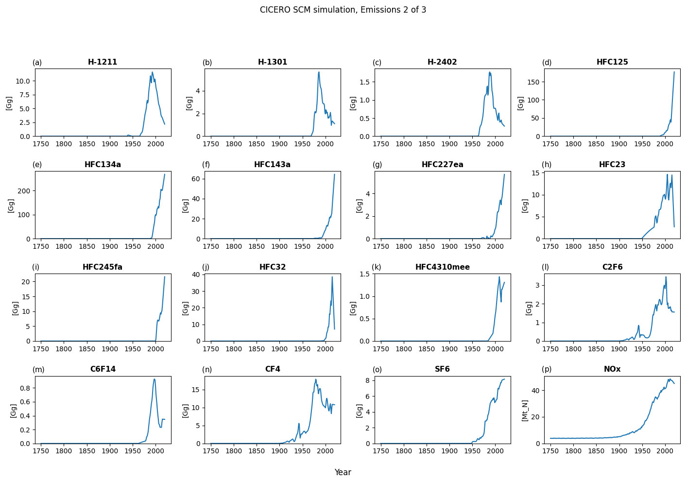
Figure A2 Default emission output plot number 2 for a run with default parameters of the historical emissions up to 2014 and the ssp245 emission year 2014 to the end of the year 2020 – all from RCMIP (Nicholls et al., 2020).

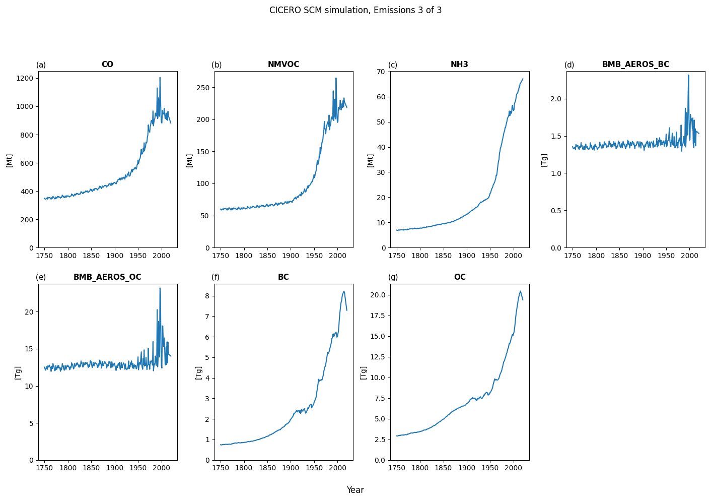
Figure A3 Default emission output plot number 3 for a run with default parameters of the historical emissions up to 2014 and the ssp245 emission year 2014 to the end of the year 2020 – all from RCMIP (Nicholls et al., 2020).

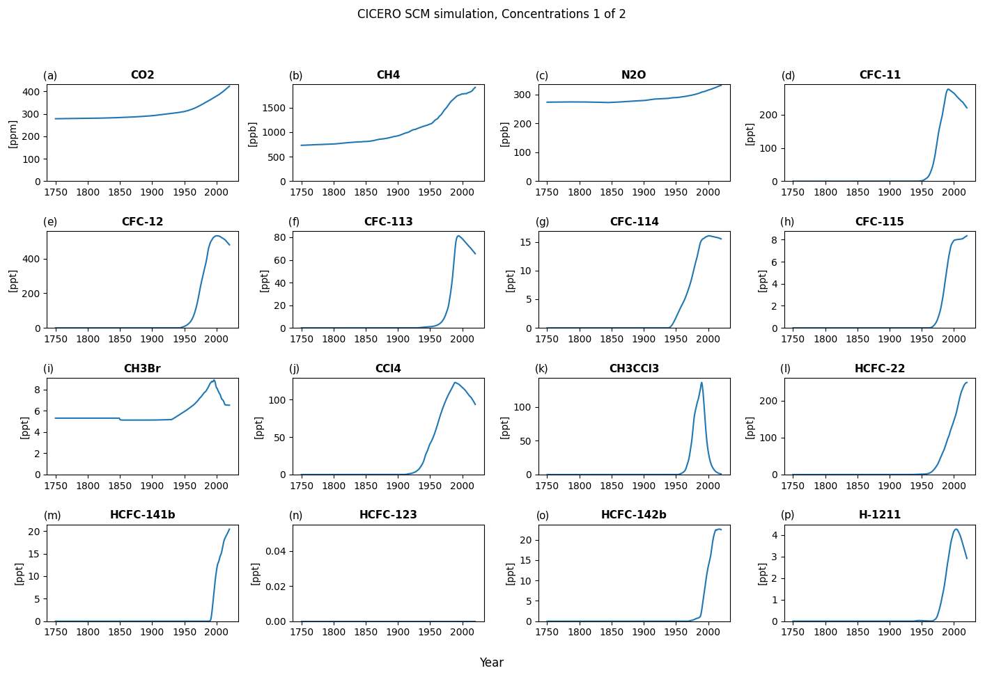
Figure A4 Default concentration output plot number 1 for a run with default parameters of the historical emissions up to 2014 and the ssp245 emission year 2014 to the end of the year 2020 – all from RCMIP (Nicholls et al., 2020). The input dataset did not include data for HCFC-123; hence, the value for this gas is zero throughout.

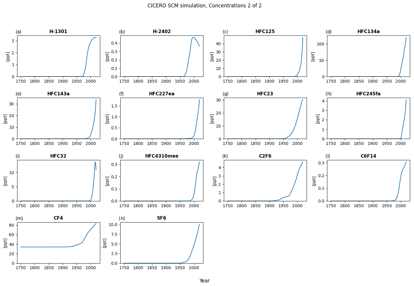
Figure A5 Default concentration output plot number 2 for a run with default parameters of the historical emissions up to 2014 and the ssp245 emission year 2014 to the end of the year 2020 – all from RCMIP (Nicholls et al., 2020).

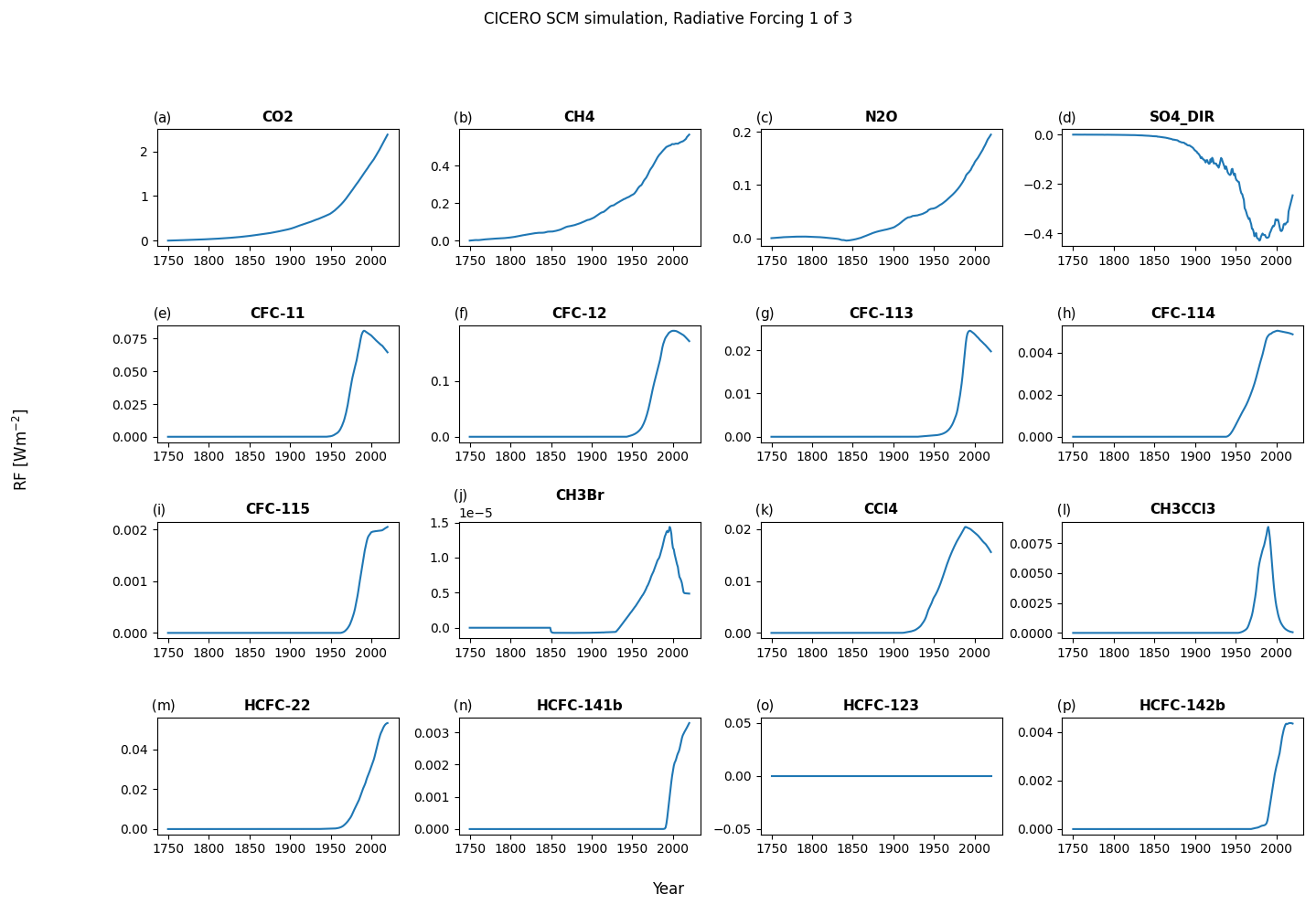
Figure A6 Default forcing output plot number 1 for a run with default parameters of the historical emissions up to 2014 and the ssp245 emission year 2014 to the end of the year 2020 – all from RCMIP (Nicholls et al., 2020). The input dataset did not include data for HCFC-123; hence, the value for this gas is zero throughout.

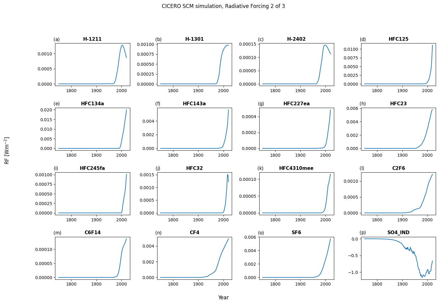
Figure A7 Default forcing output plot number 2 for a run with default parameters of the historical experiment emissions up to 2014 and the ssp245 emission year 2014 to the end of the year 2020 – all from RCMIP (Nicholls et al., 2020).

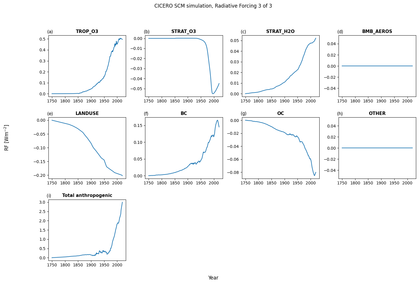
Figure A8 Default forcing output plot number 3 for a run with default parameters of the historical emissions up to 2014 and the ssp245 emission year 2014 to the end of the year 2020 – all from RCMIP (Nicholls et al., 2020). The default settings for the model have qbmb as the forcing scaling for biomass burning aerosols set to zero; hence, the BMB_AEROS forcing time series is zero throughout.

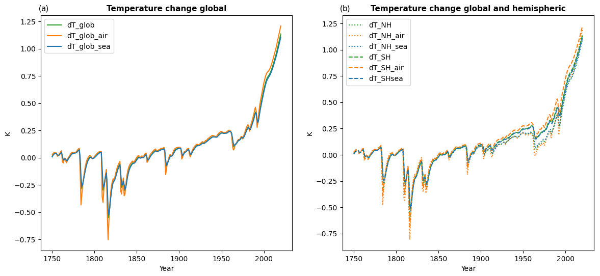
Figure A9 Default temperature change since 1750 output plot for a run with default parameters of the historical emissions up to 2014 and the ssp245 emission year 2014 to the end of the year 2020 – all from RCMIP (Nicholls et al., 2020).

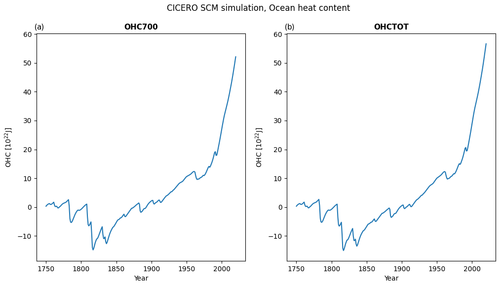
Figure A10 Default output plot of ocean heat content change since 1750 for a run with default parameters of the historical emissions up to 2014 and the ssp245 emission year 2014 to the end of the year 2020 – all from RCMIP (Nicholls et al., 2020).

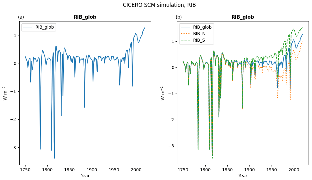
Figure A11 Default plot of radiative imbalance change since 1750 for a run with default parameters of the historical emissions up to 2014 and the ssp245 emission year 2014 to the end of the year 2020 – all from RCMIP (Nicholls et al., 2020).

Appendix B: Natural emission estimates for CH₄ and N₂O

CH₄ and N₂O both have considerable natural emission contributions (Saunois et al., 2020; Tian et al., 2020). In the model, the time series of these can be fed as separate files or dataset time series to the model instance. If not sent, a flat natural emission value from the gaspam_file will be sent. However, using a flat natural emission time series will rarely give a good match to observed concentrations, so the model also comes with a preprocessing script to generate a natural emission time series. Using a precalculated time series from a different model setup, or input dataset, will lead to different fits to the concentration time series for both components. But a finely tuned input time series will also make the calculation of the emissions to the concentration for these species superfluous, as the natural emissions are constructed to fit whatever is missing from the anthropogenic distribution, and the run will effectively be concentration-driven for these components.

In the Fortran version, the method for calculating the natural emission time series used a calibration-per-time-step method that iterated and adjusted the natural emissions from the previous step by 5 % until the concentration matched with <5 % discrepancy. As we know that we have an exact solution for converting emissions to concentrations in each time step, we can solve the equation exactly for the missing emissions in each time step for a much more efficient, though somewhat more noisy, solution. Both options are available as options from the precalculate_natural_emissions.py script in the scripts/prescripts subfolder. When the historical data finish, the future value of natural emissions is, however, assumed constant with a value that is the mean of the last 11 values. Figure A1 shows these estimates from CMIP6 (Smith et al., 2021b) concentration data, as used throughout this article, alongside the input anthropogenic emissions and the flat emissions from the default gaspam_file.

For CH₄, the amount of estimated natural emissions will vary significantly with the choice of lifetime mode, as the natural emissions are effectively masking over whatever is needed to make up the expected concentration time series. For now, this means that when running the model with estimated natural emissions, we are effectively only modeling CH₄ and N₂O forcing from concentrations in the historical period. The choice of lifetime mode may play a much larger part when natural emissions are unknown and estimated using a flat background value or a flat mean as the script calculates for the future. Figure A2 shows how the lifetime of CH₄ evolves using different lifetime modes. It also displays how different the natural emission estimates are depending on which lifetime mode is chosen.

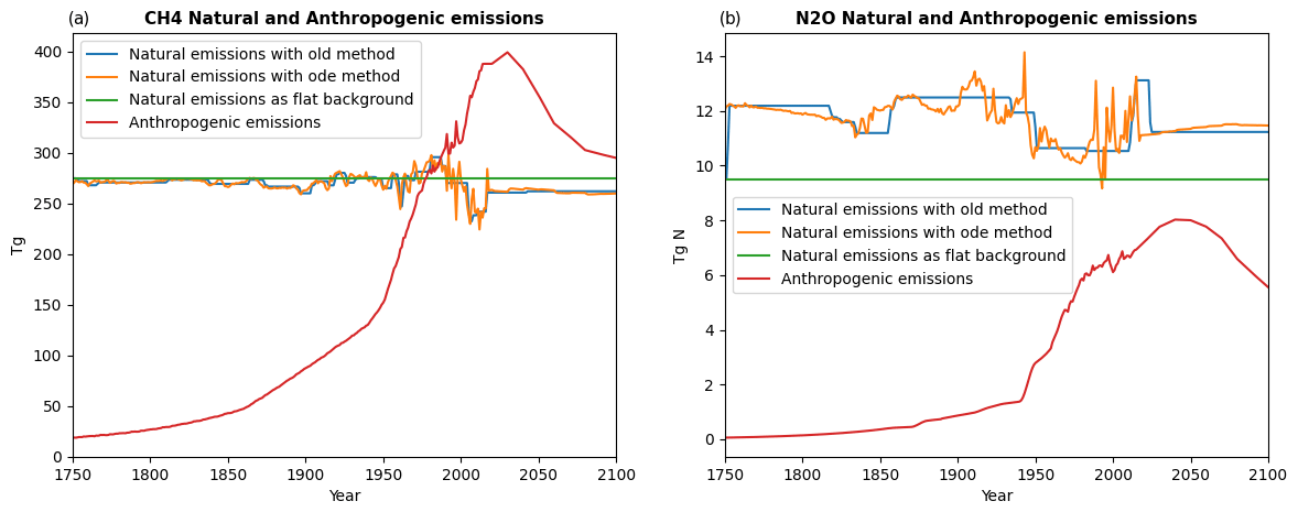
Figure B1 Time series of the estimated natural emission and anthropogenic input emissions for the historical and the ssp245 scenario for CH₄ and N₂O. The old data are data constructed using the method used to make natural emissions for the Fortran model. The ode method is using a script that is included with the Python version and is reliant on the exact solution. In both cases, the “TAR” lifetime mode for CH₄ is used for the estimates. The flat background is the flat natural emission value from the gaspam_file (Table 3).

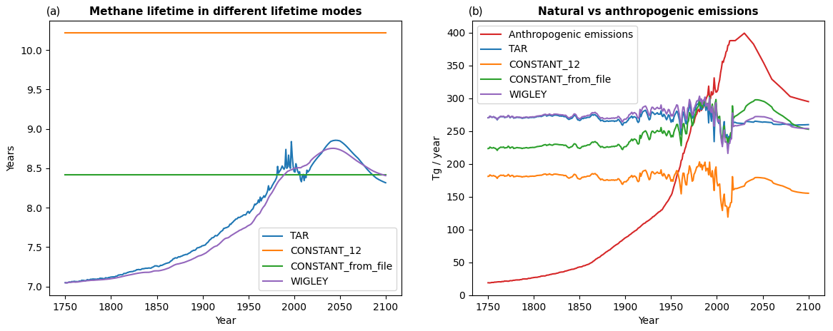
Figure B2 CH₄ lifetime time series with different lifetime modes in the ssp245 scenario in panel (a). In panel (b), the corresponding estimated lifetime emissions are made to match the concentration time series throughout the span of the experiment. The time series of the anthropogenic emissions is also shown.

Appendix C: Upwelling diffusion model equations

The equations used to describe the how energy is exchanged through the ocean system can be found in Appendix B in Schlesinger et al. (1992). They consist of differential equation sets for each of the layers in the ocean, accounting for all processes transporting heat in and out of the layer in each hemisphere. The equation for each hemisphere is completely symmetrical, so we will state only the equations for the Northern Hemisphere here for simplicity. The equations include terms relating to heat transfer between the hemispheres, and these terms are even included in the code and scaled by the atmospheric interhemispheric heat exchange parameter β_a (ebbeta). However, we will omit these terms here, as the equations simplify without them, and the parameter is mostly not used.

In the mixed (uppermost) ocean layer, the equation reads

$$\begin{array}{}\text{(C1)}& \begin{array}{rl}{\mathit{\gamma }}_{\mathrm{N}}\mathit{\rho }c\mathrm{\Delta }{z}_{\mathrm{1}}{\displaystyle \frac{\mathit{\delta }{T}_{\mathrm{1}}}{\mathit{\delta }t}}& =q-\mathit{\lambda }{T}_{\mathrm{1}}+\mathrm{2}{\mathit{\gamma }}_{\mathrm{N}}\mathit{\rho }{c}_p\mathit{\kappa }{\displaystyle \frac{T_{\mathrm{2}}-T_{\mathrm{1}}}{\mathrm{\Delta }{z}_{\mathrm{2}}}}\\ & +{\mathit{\gamma }}_{\mathrm{N}}\mathit{\rho }{c}_{p}W\left(T_{\mathrm{1}}-T_{\mathrm{P}}\right)-{\mathit{\gamma }}_{\mathrm{N}}{\mathit{\beta }}_{\mathrm{o}}\left(T_{\mathrm{1}}-T_{\mathrm{1},\mathrm{S}}\right),\end{array}\end{array}$$

where ${\mathit{\gamma }}_{\mathrm{N}}={\mathit{\sigma }}_{\mathrm{N}}+\frac{\mathit{\lambda }}{{\mathit{\lambda }}_{\mathrm{a},\mathrm{o}}}$, with σ_N as the Northern Hemisphere ocean fraction (foan), λ_a,o (rlamdo) as the air–sea heat exchange parameter, and λ as the equilibrium climate sensitivity divided by 2xCO₂ radiative forcing (see Table 4 for details and units). Both temperature and forcing values denote changes from the temperature and forcing at the start of the model run rather than absolute temperatures. Subscript numbers denote the ocean layer number, counted from the top, so layer 1 is the mixed layer. All quantities are the versions of the quantities in the Northern Hemisphere non-polar ocean unless otherwise specified. T_1,S is the temperature in the Southern Hemisphere, and T_P is the Northern Hemisphere polar ocean temperature that is assumed to change according to B8 in Schlesinger et al. (1992), i.e., just following the change in the main ocean temperature mixed layer times Π (the cpi parameter in Table 4).

$$\begin{array}{}\text{(C2)}& T_p=\mathrm{\Pi }\cdot T_{\mathrm{1}}\end{array}$$

q is the Northern Hemisphere forcing (in W m⁻²), ρ is the seawater density (1030 kg m³), c_p is the specific heat capacity of seawater (3.997×10³ J kg⁻¹ K⁻¹), and Δz_l is the height of layer l in meters. κ is the vertical heat diffusivity (akapa), β_o is the oceanic interhemispheric heat exchange rate (beto), and W is the upwelling rate. These three are tunable parameters (see Table 4 for details and units). Finally, when the parameter threshtemp is non-zero, the upwelling rate W, is not equal to the parameter W in Table 4, but it is rather given as

$$\begin{array}{}\text{(C3)}& W=W_{\text{Table 4}}\cdot \left(\mathrm{1}-{\displaystyle \frac{\mathrm{10}}{\mathrm{3}}}\cdot {\displaystyle \frac{T_{\mathrm{1}}}{T_{\mathrm{thres}}}}\right);\end{array}$$

that is, the threshtemp parameter is the mixed-layer temperature change at which the upwelling velocity decreases by 30 %. This decrease in the upwelling velocity was not included in the model described in Schlesinger et al. (1992) but is an update based on the work of Raper et al. (2001).

To simplify the equations, atmospheric transport between the hemispheres is assumed to be zero in this derivation, though it is included in the code, and its strength is controlled by the parameter ebbeta (β_a).

The left-hand side represents the rate of change in the energy in the mixed layer, where the γ_N factor accounts for heat exchange between the ocean and the atmosphere (and when β_a is included also with atmospheric interhemispheric heat exchange). Examining the terms on the right-hand side, they represent radiative forcing, then the temperature longwave radiation and climate feedback, then the vertical diffusion heat transport to the layer below, then the vertical advective heat transport into the polar ocean, and, finally, the interhemispheric heat transport. The polar ocean temperature is assumed to be ΠT₁ throughout.

For all internal ocean layers, the equation is

$$\begin{array}{}\text{(C4)}& \begin{array}{rl}\mathit{\rho }{c}_p\mathrm{\Delta }{z}_k{\displaystyle \frac{\mathit{\delta }{T}_k}{\mathit{\delta }t}}& =\mathit{\rho }{c}_p\left[\mathrm{2}\mathit{\kappa }{\displaystyle \frac{T_{k+\mathrm{1}}-T_k}{\left(\mathrm{\Delta }{z}_k+\mathrm{\Delta }{z}_{k+\mathrm{1}}\right)}}+W\cdot T_{k+\mathrm{1}}\right]\\ & -\mathit{\rho }{c}_p[\mathrm{2}\mathit{\kappa }{\displaystyle \frac{T_k-T_{k-\mathrm{1}}}{\left(\mathit{\delta }\mathrm{\Delta }{z}_k+\mathrm{\Delta }{z}_{k-\mathrm{1}}\right)}}+W\\ & \cdot (\mathit{\delta }{T}_k+(\mathrm{1}-\mathit{\delta }\left)T_{k-\mathrm{1}}\right)]-{\mathit{\beta }}_{\mathrm{o}}\left(T_k-T_{k,S}\right).\end{array}\end{array}$$

Here, we have the rate of change in the energy per area in the layer on the left, diffusion and advection with the layer below first and then diffusion and advection with the layer above, and, finally, the interhemispheric heat transport across the horizontal boundary. The δ value in the denominator of the diffusion term and in the second advection term is zero for the uppermost of the layers and one otherwise. In the equation for the Southern Hemisphere, this last term will also be scaled by the ratio between the two ocean surfaces to ensure that an equal amount of heat is accounted for, as seen from both hemispheres. Note also that in the original formulation in Schlesinger et al. (1992), the advection terms did not depend on the temperature in the layer from which the advection came; i.e., they were not dependent on the form given here of $\mathit{\rho }{c}_p\cdot W\cdot T_{k+\mathrm{1}}$ and $\mathit{\rho }{c}_p\cdot W\cdot T_k$ but rather on the average temperature between the layer from which the advection came and the one it advected into, i.e., on the form $\mathit{\rho }{c}_p\cdot W\frac{T_{k+\mathrm{1}}+T_k}{\mathrm{2}}$ and $\mathit{\rho }{c}_p\cdot W\frac{T_{k-\mathrm{1}}+T_k}{\mathrm{2}}$. The same was true for the advection out of the bottom layer (see Eq. C5).

For the ocean bottom layer L, the equation reads

$$\begin{array}{}\text{(C5)}& \begin{array}{rl}\mathit{\rho }{c}_p\mathrm{\Delta }{z}_{\mathrm{L}}{\displaystyle \frac{\mathit{\delta }{T}_{\mathrm{L}}}{\mathit{\delta }t}}& =-\mathit{\rho }{c}_p\left[\mathrm{2}\mathit{\kappa }{\displaystyle \frac{T_{\mathrm{L}}-T_{L-\mathrm{1}}}{\left(\mathrm{\Delta }{z}_{\mathrm{L}}+\mathrm{\Delta }{z}_{L-\mathrm{1}}\right)}}+W\cdot T_{\mathrm{L}}\right]\\ & +\mathit{\rho }{c}_p{\mathrm{WT}}_{\mathrm{P}}-{\mathit{\beta }}_{\mathrm{o}}\left(T_{\mathrm{L}}-T_{\mathrm{L},\mathrm{S}}\right),\end{array}\end{array}$$

where there is no longer any heat transported from the layer below. As there is none, however, we also account for the transport of heat from the bottom of the polar ocean and transport to the Southern Ocean. In other words, in the model, heat is transferred into the polar ocean at the top and transported back from it at the bottom layer.

Now, for the solution of this equation set in the code, the solution involves a separation of terms. First for the forcing, interhemispheric heat exchange terms, and polar heat exchange terms, a simple forward Euler solution, $\mathit{\delta }{T}_k\left(t\right)\approx T_k\left(t\right)-T_k(t-\mathrm{1})$, is employed in gathering all these terms in one and solving for them in all layers first. These are then added to the equations and can be viewed as constant terms in the further differentiation. Then the climate feedback, diffusion, and advection terms are combined in a backward implicit Euler calculation. That is to say, the equations are solved, assuming all these terms are given for the current time step, and we solve the equations for them.

We rewrite the top layer in Eq. (C1) as

$$\begin{array}{}\text{(C6)}& {\displaystyle }\begin{array}{rl}{\mathit{\gamma }}_{\mathrm{N}}\mathit{\rho }{c}_p\mathrm{\Delta }{z}_{\mathrm{1}}{\displaystyle \frac{\mathit{\delta }{T}_{\mathrm{1}}}{\mathit{\delta }t}}& =q-\mathit{\lambda }{T}_{\mathrm{1}}+\mathrm{2}{\mathit{\gamma }}_{\mathrm{N}}\mathit{\rho }{c}_p\mathit{\kappa }{\displaystyle \frac{T_{\mathrm{2}}-T_{\mathrm{1}}}{\mathrm{\Delta }{z}_{\mathrm{2}}}}\\ & +{\mathit{\gamma }}_{\mathrm{N}}\mathit{\rho }{c}_{p}W\left(T_{\mathrm{1}}-T_{\mathrm{P}}\right)\\ & -{\mathit{\gamma }}_{\mathrm{N}}{\mathit{\beta }}_{\mathrm{o}}\left(T_{\mathrm{1}}-T_{\mathrm{1},\mathrm{S}}\right)\end{array}\text{(C7)}& {\displaystyle }\begin{array}{rl}{\mathit{\gamma }}_{\mathrm{N}}& \mathit{\rho }{c}_p\mathrm{\Delta }{z}_{\mathrm{1}}{\displaystyle \frac{T_{\mathrm{1}}\left(t\right)-T_{\mathrm{1}}\left(t-\mathrm{1}\right)}{\mathrm{d}t}}-\mathrm{2}{\mathit{\gamma }}_{\mathrm{N}}\mathit{\rho }{c}_p\mathit{\kappa }{\displaystyle \frac{T_{\mathrm{2}}-T_{\mathrm{1}}}{\mathrm{\Delta }{z}_{\mathrm{2}}}}\\ & -{\mathit{\gamma }}_{\mathrm{N}}\mathit{\rho }{c}_{p}W{T}_{\mathrm{1}}=q-\mathit{\lambda }{T}_{\mathrm{1}}-{\mathit{\gamma }}_{\mathrm{N}}\mathit{\rho }{c}_{p}W\mathrm{\Pi }{T}_{\mathrm{1}}-\\ & {\mathit{\gamma }}_{\mathrm{N}}{\mathit{\beta }}_{\mathrm{o}}\left(T_{\mathrm{1}}-T_{\mathrm{1},\mathrm{S}}.\right)\end{array}\end{array}$$

Unless otherwise stated, the left-hand side (LHS) is time t, and the right-hand side (RHS) is time t−1. Dividing by $\frac{{\mathit{\gamma }}_{\mathrm{N}}\mathit{\rho }{c}_p\mathrm{\Delta }{z}_{\mathrm{1}}}{\mathrm{d}t}$,

$$\begin{array}{}\text{(C8)}& {\displaystyle }\begin{array}{rl}{T}_{\mathrm{1}}\left(t\right)& -T_{\mathrm{1}}\left(t-\mathrm{1}\right)-{\displaystyle \frac{\mathrm{2}\mathit{\kappa }\mathrm{d}t}{\mathrm{\Delta }{z}_{\mathrm{1}}\mathrm{\Delta }{z}_{\mathrm{2}}}}\left(T_{\mathrm{2}}-T_{\mathrm{1}}\right)-{\displaystyle \frac{W\mathrm{d}t}{\mathrm{\Delta }{z}_{\mathrm{1}}}}{T}_{\mathrm{1}}\\ & ={\displaystyle \frac{q\mathrm{d}t}{{\mathit{\gamma }}_{\mathrm{N}}\mathit{\rho }{c}_p\mathrm{\Delta }{z}_{\mathrm{1}}}}-{\displaystyle \frac{\mathit{\lambda }\mathrm{d}t}{{\mathit{\gamma }}_{\mathrm{N}}\mathit{\rho }{c}_p\mathrm{\Delta }{z}_{\mathrm{1}}}}{T}_{\mathrm{1}}-{\displaystyle \frac{W\mathrm{\Pi }\mathrm{d}t}{\mathrm{\Delta }{z}_{\mathrm{1}}}}{T}_{\mathrm{1}}\\ & -{\displaystyle \frac{{\mathit{\beta }}_{\mathrm{o}}\mathrm{d}t}{\mathit{\rho }{c}_p\mathrm{\Delta }{z}_{\mathrm{1}}}}\left(T_{\mathrm{1}}-T_{\mathrm{1},\mathrm{S}}\right)\end{array}\text{(C9)}& {\displaystyle }\begin{array}{rl}& \left(\mathrm{1}+{\displaystyle \frac{\mathit{\lambda }\mathrm{d}t}{{\mathit{\gamma }}_{\mathrm{N}}\mathit{\rho }{c}_p\mathrm{\Delta }{z}_{\mathrm{1}}}}+{\displaystyle \frac{\mathrm{2}\mathit{\kappa }\mathrm{d}t}{\mathrm{\Delta }{z}_{\mathrm{1}}\mathrm{\Delta }{z}_{\mathrm{2}}}}-{\displaystyle \frac{W\mathrm{d}t}{\mathrm{\Delta }{z}_{\mathrm{1}}}}\right)T_{\mathrm{1}}\\ & -{\displaystyle \frac{\mathrm{2}\mathit{\kappa }\mathrm{d}t}{\mathrm{\Delta }{z}_{\mathrm{1}}\mathrm{\Delta }{z}_{\mathrm{2}}}}{T}_{\mathrm{2}}=\left(\mathrm{1}-{\displaystyle \frac{W\mathrm{\Pi }\mathrm{d}t}{\mathrm{\Delta }{z}_{\mathrm{1}}}}-{\displaystyle \frac{{\mathit{\beta }}_{\mathrm{o}}\mathrm{d}t}{\mathit{\rho }{c}_p\mathrm{\Delta }{z}_{\mathrm{1}}}}\right)T_{\mathrm{1}}\\ & +{\displaystyle \frac{{\mathit{\beta }}_{\mathrm{o}}\mathrm{d}t}{\mathit{\rho }{c}_p\mathrm{\Delta }{z}_{\mathrm{1}}}}{T}_{\mathrm{1},\mathrm{S}}+{\displaystyle \frac{q\mathrm{d}t}{{\mathit{\gamma }}_{\mathrm{N}}\mathit{\rho }{c}_p\mathrm{\Delta }{z}_{\mathrm{1}}}}.\end{array}\end{array}$$

Note that, for shorthand, LHS is time t, and RHS is time t−1.

The equation set can, in principle, be written in this way for the various layers:

$$\begin{array}{}\text{(C10)}& \begin{array}{rl}{b}_{\mathrm{1}}{T}_{\mathrm{1}}+c_{\mathrm{1}}{T}_{\mathrm{2}}& =d_{\mathrm{1}},a_k{T}_{k-\mathrm{1}}+b_k{T}_k+c_k{T}_{k+\mathrm{1}}=d_k,\\ & a_{\mathrm{L}}{T}_{L-\mathrm{1}}+b_{\mathrm{L}}{T}_{\mathrm{L}}=d_{\mathrm{L}}.\end{array}\end{array}$$

In the code, we go through the equations and find the coefficients a_k, b_k, and c_k. The d_k terms are the results of the forward-Euler solution for the horizontal transport. This now defines a banded matrix problem and can be solved using a suitable banded matrix solver.

Following this approach, the coefficients a₁, b₁, and d₁ are

$$\begin{array}{}\text{(C11)}& \begin{array}{rl}{b}_{\mathrm{1}}& =\mathrm{1}+{\displaystyle \frac{\mathit{\lambda }\mathrm{d}t}{{\mathit{\gamma }}_{\mathrm{N}}\mathit{\rho }c\mathrm{\Delta }{z}_{\mathrm{1}}}}+{\displaystyle \frac{\mathrm{2}\mathit{\kappa }\mathrm{d}t}{\mathrm{\Delta }{z}_{\mathrm{1}}\mathrm{\Delta }{z}_{\mathrm{2}}}}-{\displaystyle \frac{W\mathrm{d}t}{\mathrm{\Delta }{z}_{\mathrm{1}}}},\\ & c_{\mathrm{1}}=-{\displaystyle \frac{\mathrm{2}\mathit{\kappa }dt}{\mathrm{\Delta }{z}_{\mathrm{1}}\mathrm{\Delta }{z}_{\mathrm{2}}}},\\ & d_{\mathrm{1}}=\left(\mathrm{1}-{\displaystyle \frac{\mathrm{\Pi }W\mathrm{d}t}{\mathrm{\Delta }{z}_{\mathrm{1}}}}-{\displaystyle \frac{{\mathit{\beta }}_{\mathrm{o}}\mathrm{d}t}{\mathit{\rho }{c}_p\mathrm{\Delta }{z}_{\mathrm{1}}}}\right)T_{\mathrm{1}}\left(t-\mathrm{1}\right)\\ & +{\displaystyle \frac{{\mathit{\beta }}_{\mathrm{o}}\mathrm{d}t}{\mathit{\rho }{c}_p\mathrm{\Delta }{z}_{\mathrm{1}}}}{T}_{\mathrm{1},\mathrm{S}}\left(t-\mathrm{1}\right)+{\displaystyle \frac{q\mathrm{d}t}{{\mathit{\gamma }}_{\mathrm{N}}\mathit{\rho }{c}_p\mathrm{\Delta }{z}_{\mathrm{1}}}},\end{array}\end{array}$$

where q is now the mean forcing over the preceding year.

Performing similar transformations to those for the top layer in Eq. (C4), the coefficients for the internal layers a_k, b_k, c_k, and d_k become

$$\begin{array}{}\text{(C12)}& \begin{array}{rl}{a}_k& =-{\displaystyle \frac{\mathrm{2}\mathit{\kappa }\mathrm{d}t}{\mathrm{\Delta }{z}_k\left(\mathit{\delta }\mathrm{\Delta }{z}_k+\mathrm{\Delta }{z}_{k-\mathrm{1}}\right)}}+(\mathrm{1}-\mathit{\delta }){\displaystyle \frac{W\mathrm{d}t}{\mathrm{\Delta }{z}_k}},\\ & b_k=\mathrm{1}+{\displaystyle \frac{\mathrm{2}\mathit{\kappa }\mathrm{d}t}{\mathrm{\Delta }{z}_k\left(\mathrm{\Delta }{z}_{k-\mathrm{1}}+\mathit{\delta }\mathrm{\Delta }{z}_k\right)}}\\ & +{\displaystyle \frac{\mathrm{2}\mathit{\kappa }\mathrm{d}t}{\mathrm{\Delta }{z}_k\left(\mathrm{\Delta }{z}_{k+\mathrm{1}}+\mathrm{\Delta }{z}_k\right)}}+\mathit{\delta }{\displaystyle \frac{W\mathrm{d}t}{\mathrm{\Delta }{z}_k}},\\ & c_k=-{\displaystyle \frac{\mathrm{2}\mathit{\kappa }\mathrm{d}t}{\mathrm{\Delta }{z}_k(\mathrm{\Delta }{z}_{k+\mathrm{1}}+\mathrm{\Delta }{z}_k)}}-{\displaystyle \frac{W\mathrm{d}t}{\mathrm{2}\mathrm{\Delta }{z}_k}},\\ & d_k=\left(\mathrm{1}-{\displaystyle \frac{{\mathit{\beta }}_{\mathrm{o}}\mathrm{d}t}{\mathit{\rho }{c}_p\mathrm{\Delta }{z}_k}}\right)T_k\left(t-\mathrm{1}\right)\\ & +{\displaystyle \frac{{\mathit{\beta }}_{\mathrm{o}}\mathrm{d}t}{\mathit{\rho }{c}_p\mathrm{\Delta }{z}_k}}{T}_{k,S}\left(t-\mathrm{1}\right),\end{array}\end{array}$$

where δ in the expression for a_k, and b_k is zero for the second layer and one otherwise.

And for the bottom layer (from Eq. C5),

$$\begin{array}{}\text{(C13)}& \begin{array}{rl}{a}_{\mathrm{L}}& =-{\displaystyle \frac{\mathrm{2}\mathit{\kappa }\mathrm{d}t}{\mathrm{\Delta }{z}_{\mathrm{L}}(\mathrm{\Delta }{z}_{\mathrm{L}}+\mathrm{\Delta }{z}_{L-\mathrm{1}})}},\\ & b_{\mathrm{L}}=\mathrm{1}+{\displaystyle \frac{\mathrm{2}\mathit{\kappa }\mathrm{d}t}{\mathrm{\Delta }{z}_{\mathrm{L}}(\mathrm{\Delta }{z}_{\mathrm{L}}+\mathrm{\Delta }{z}_{L-\mathrm{1}})}}+{\displaystyle \frac{W\mathrm{d}t}{\mathrm{\Delta }{z}_{\mathrm{L}}}},c_{\mathrm{L}}=\mathrm{0},\\ & d_{\mathrm{L}}=\left(\mathrm{1}-{\displaystyle \frac{{\mathit{\beta }}_{\mathrm{o}}\mathrm{d}t}{\mathit{\rho }{c}_p\mathrm{\Delta }{z}_{\mathrm{L}}}}\right)T_{\mathrm{L}}\left(t-\mathrm{1}\right)\\ & +{\displaystyle \frac{{\mathit{\beta }}_{\mathrm{o}}\mathrm{d}t}{\mathit{\rho }{c}_p\mathrm{\Delta }{z}_{\mathrm{L}}}}{T}_{\mathrm{L},\mathrm{S}}\left(t-\mathrm{1}\right)+{\displaystyle \frac{\mathrm{\Pi }W\mathrm{d}t}{\mathrm{\Delta }{z}_{\mathrm{L}}}}{T}_{\mathrm{1}}\left(t-\mathrm{1}\right).\end{array}\end{array}$$